Finite Element Analysis-Based Assessment of Damage Parameters for Ultra-Low-Cycle Fatigue Behavior of Structural Steels

Abstract

Steel structures subjected to earthquakes or extreme cyclic loadings may undergo extensive damage and fractures due to ultra-low-cycle fatigue (ULCF). Although assessments of damage initiation and evolution parameters have been carried out for some steels exposed to low-cycle fatigue, so far, these parameters for structural steels exposed to ULCF have neither been sufficiently studied nor quantified. Accordingly, this paper provides the results of finite element analysis (FEA) concerning the ULCF behaviors of S355 and S690 steel specimens. Calibration of the damage parameters is performed in SIMULIA Abaqus 6.11 FEA software using a direct cyclic algorithm and available experimental data. Kliman’s model for the hysteresis energy of cyclic loading is used to analytically verify the damage parameters. In addition, available experimental data were obtained from cyclic axial strain tests on S355 and S690 steel specimens according to the ASTM International standard E606/E606M-21. Finally, the non-linear Chaboche–Lemaitre (C–L) combined isotropic–kinematic hardening model is used for the characterization of the ULCF behavior of S355 steel in a simple cylindrical bar. It is found that the two damage initiation parameters are 5.0 and −0.8, the first damage initiation parameter is dominant when modeling the number of cycles to failure, and the second damage initiation parameter is a material constant.

1. Introduction

The Vöhler curve for any structural steel indicates the number of loading cycles the steel can withstand before failure [1]. It is the dependency of the magnitude of an alternating/cyclic stress on the number of loading cycles to failure for a given steel (or any other material), and it can generally be divided into the following five modes [2,3]: monotonic fracture, ultra-low-cycle fatigue (ULCF), low-cycle fatigue, finite life fatigue, and high-cycle fatigue. Monotonic fracture and ULCF concern damages under high-magnitude stress close to ultimate strength and quite a low number of loading cycles. Macro-level plastic deformation, fatigue crack initiation, and fatigue crack growth occur in every loading cycle. This evolutionary process of damage ends in failure. In particular, structural engineering problems with a fatigue life ranging from a few to one hundred loading cycles belong to the ULCF life and are correlated with a high level of seismic activity [2,4]. Until today, a large number of steel structures of various buildings and bridges were cracked at the beam-to-column connections due to earthquakes or extreme cyclic loadings [4]. In order to study the behavior of steel structures under such mechanical loads, damage initiation and evolution parameters need to be assessed using relevant and standardized models [5].

Models for predicting the ULCF life (that is, behavior or evolution) of structural steels that have been developed until mid-2023 were reviewed in [6,7]. According to [6,7], these ductile fracture models can be divided into the following three types: (1) microscopic models based on crack growth and cohesive zone, (2) models based on porous plasticity, and (3) models based on continuum damage mechanics. All research results on the prediction of the ULCF evolution of structural steels published after the reviews [6,7] can be regarded as relevant and state of the art.

Specifically, a ULCF prediction model for structural steels that considers the effects of loading amplitude, loading frequency, and surface roughness was developed in [8]. Based on a reasonable selection of parameters, the model proposed in [8] estimated ULCF life within an error band of ±15%. ULCF fracture of thick-walled steel bridge piers was studied in [9]. The models used in [9] predicted the ULCF fracture initiation life of the piers with an average discrepancy of 7.14%. A cyclic Gurson–Tvergaard–Needleman model for the ULCF analysis of structural steels was proposed in [10]. According to [10], the proposed model can provide a ULCF prediction of materials with a satisfactory level of accuracy. The fracture performance and some damage parameters of K460D steel and ER55-G welds under ULCF conditions after exposure to fire were experimentally and numerically analyzed in [11]. The simulated results from [11] aligned closely with the associated experimental data. The ULCF performance of steel butt-welded joints affected by corrosion were modeled in [12]. Specifically, corrosion could reduce the ULCF life by as much as 77.31% [12].

Seismic damage behaviors of some structural steels using various constitutive and damage models were analyzed in [13]. It was shown in [13] that various cyclic loading protocols can cause various cases of cumulative damage evolution. The effect of pre-tension on bolted flange plate connections was investigated in [14]. In this study, a ULCF failure index was used to evaluate the connection failure location and the cycle in which a joint reaches its ultimate capacity. A simplified method based on a fiber element model to evaluate ULCF damage of unstiffened steel piers was proposed in [15]. An application of the proposed method in [14] for predicting half-cycles of random cyclic loading resulted in a mean absolute error of 3.05%. A continuous damage model to assess the ULCF behavior of structural steels and weld metals was developed and applied in [16]. The model used in [16] provided credible predictions for crack initiation, crack propagation, and fatigue life. Based on an existing ductile fracture model, the Coffin–Manson model, and the Miner law, a ULCF life prediction model for steels and other alloys was proposed in [17]. In this case, the average error for ULCF life predicted by the proposed model was 12.6%.

The effect of the loading sequence on the ULCF performance of all-steel buckling-restrained braces was considered in [18]. Some ULCF parameters for corroded Q235 steel samples under monotonic and cyclic loadings were determined in [19]. According to [19], corrosion may be more destructive in cyclic loading than in monotonic loading. ULCF life predictions of structural steels using synthetic data, artificial neural networks, and multi-fidelity deep neural networks were performed in [20]. The results obtained in [20] showed that applications of machine learning models for ULCF life predictions of structural steels can reduce the cost of parameter calibration. ULCF behaviors for three different types of structural steels were compared in [21]. In addition to these comparisons, the effectiveness of different models for determining the ULCF behaviors of structural steels was successfully demonstrated in [21]. Based on this state-of-the-art literature review, it is obvious that the damage initiation and evolution parameters appearing in [5] have not yet been quantified for structural steels exposed to ULCF. The practical significance of the damage parameters is precisely related to the modeling of real structural elements, such as beam-to-column connections and truss structures. So, this is a research gap that need to be filled. Addressing the identified gap can be considered the first contribution of this study.

In this paper, the ULCF behaviors of specimens made of the structural steels S355 and S690 and exposed to cyclic axial strains in the plastic range are analyzed. S355 steel was chosen because it belongs to the group of ordinary structural steels whose usage is the most common, while S690 steel was chosen because it belongs to the group of structural steels with improved yield strength whose applications in the construction industry are extensive. ULCF behavior was achieved by the dominance of plastic strain over elastic strain, as well as by the number of cycles to failure lower than one hundred. Traditionally, the fatigue limit for these specimens should be determined using a method based on the Wöhler curve, that is, dependency. However, this common method has not been applied because it does not establish a correlation between any individual loading cycle and the rate of damage. To overcome this issue, the direct cyclic algorithm from SIMULIA Abaqus 6.11 software [22] was utilized in this study to compute stabilized hysteretic responses of the specimens directly. SIMULIA Abaqus 6.11 is a software package for finite element analysis (FEA) and computer-aided engineering.

According to [22,23], the direct cyclic algorithm combines a Fourier series approximation with a time integration scheme (for the non-linear UCLF behavior of the specimens) to obtain the stabilized hysteretic responses iteratively using the modified Newton method. In particular, the direct cyclic algorithm was used to determine the number of cycles to the initiation of damage and the rate of damage after each individual loading cycle. Compared to other standardized models that provide total damage over the fatigue life of a material, the application of the direct cyclic algorithm to the ULCF behavior of the specimens represents an advantage, which is also another contribution of this research. Furthermore, the damage parameters of one specimen (discretized into solid eight-node hexahedrons) and one cylindrical bar (discretized into truss finite elements) were determined by applying the non-linear Chaboche–Lemaitre (C–L) combined isotropic–kinematic hardening model [24,25] in finite element method (FEM)-based simulations of cyclic axial strain tests. The application of the C–L model to this specific comparison represents the third contribution. Furthermore, the generation of damage initiation and evolution plots for 90 cycles and five different stress ratios is the fourth contribution. Finally, available experimental data were used for calibration purposes, and this research provided results that are applicable in practice.

2. Experimental Background

ULCF life parameters have typically been assessed by subjecting specific cylindrical specimens to cyclic loading. In order for the generated results to be mutually comparable, the same geometry of cylindrical specimens from S355 and S690 steels is studied. Test data related to the cylindrical S355 and S690 specimens are taken from the master’s thesis of Versaillot [26]. Versaillot prepared, tested, and analyzed the specimens according to the ASTM International standard E606/E606M-21 [27]. Some additional experimental data obtained by Vucko et al. [28] in accordance with [27] are also used for the FEA of another cylindrical S690 specimen. The necessary mechanical and kinematic properties of S355 steel are taken from [26,29], while the ones of S690 steel are taken from [30]. Then, an FEA-based assessment of the damage initiation and evolution parameters is conducted for all these specimens under ULCF conditions.

2.1. Materials and Specimens

Two S355 specimens and three S690 specimens were prepared according to the drawing shown in Figure 1. The shape and dimensions of these cylindrical specimens were selected in line with the ASTM International standard E606/E606M-21 [27]. The cross-section of the gauge of the cylindrical specimens (Section 1-1) is a circle with a diameter of 15 mm.

Table 1. Mechanical and kinematic properties of S355 and S690 structural steels.

Material	Elastic Range		Plastic Range
	$\mathit{E}$ (MPa)	$\mathsf{\nu }$ (–)	$\mathsf{\sigma }{|}_0$ (MPa)	$\mathit{C}$ (MPa)	$\mathsf{\gamma }$ (–)	${\mathit{Q}}_{\mathbf{\infty }}$ (MPa)	$\mathit{b}$ (–)
S355 [26,29]	208,000	0.3	357	8000	75	110	4
S690 [30]	207,000	0.3	540.5	38,100	153	−30	3

outlines the material properties of S355 and S690 structural steels. The parameters appearing in Table 1 are as follows: $E$ is Young’s modulus in MPa; $\nu$ is Poisson’s ratio; ${\left.\sigma \right|}_0$ is the initial value of the current size of the yield surface (half of the stress magnitude in the elastic range) in MPa; $C$ is the initial kinematic hardening modulus in MPa; $\gamma$ is the rate factor for kinematic hardening; $Q_{\infty }$ is the maximum change in yield stress for isotropic hardening in MPa; and $b$ is the rate factor for isotropic hardening.

2.2. Experimental Testing

The experiments of Versaillot [26] were performed on cylindrical S355 and S690 specimens subjected to axial cyclic strains at room temperature, using an ultimate tensile strength (UTS) load frame. These specimens were tested at a constant strain rate of 0.002 p.u./s for a loading protocol, with constant strain amplitudes of ±0.05 p.u. and ±0.07 p.u. The mechanical and kinematic properties of S355 structural steel are taken from [26,29]. These properties were obtained in a series of experiments performed on a full-scale testing frame that was mounted horizontally on the floor and hinged at the four corners by means of steel pins [29]. Two different loading protocols were applied in the experiments from [29], namely cyclic quasi-static and dynamic loadings. For S690 structural steel, the mechanical properties (from monotonic loading experiments) and kinematic parameters (calibrated based on cyclic loading experiments) are taken from [30]. The S690 specimens used in the study of Hai et al. [30] were exposed to axial cyclic strains by a universal tension, compression, and torsion fatigue testing machine (MTS 880), at room temperature as well. According to [30], these loading cycles were performed at a constant strain rate of 0.002 p.u./s and at constant strain amplitudes ranging from ±0.005 p.u. to ±0.04 p.u.

The cylindrical S690 specimen used by Vucko et al. [28] was tested and analyzed using Handfield and Dickson’s measuring method at room temperature and under of conditions of plastic strain-controlled low-cycle fatigue [31,32,33]. In this case, damage parameter identification was based on ULCF tests at a constant strain rate of 0.0005 p.u./s and at constant strain amplitudes ranging from ±0.004 p.u. to ±0.04 p.u. All these experiments were arranged according to the ASTM International standard E606/E606M-21 [27], and the number of cycles to their failure belonged to the ULCF life.

2.3. Test Results

In the previously described experiments, the following results were obtained [26,28,29,30]: (1) cyclic stress–strain curves, i.e., hysteretic responses, for the cylindrical S355 and S690 specimens; (2) a maximum stress vs. number-of-cycles-to-failure curve for one cylindrical S690 specimen; and (3) mechanical and kinematic properties of S355 and S690 structural steels. In Section 4, the hysteretic responses and the maximum stress vs. number-of-cycles-to-failure curve are compared with the associated simulated data, while the mechanical and kinematic properties are used as input data for FEM-based simulations in SIMULIA Abaqus 6.11 software [22]. These comparisons are further used to analyze the damage initiation and evolution parameters.

3. Theoretical Background and Mathematical Modeling

3.1. Theoretical Background

The application of FEA requires mathematical models that can accurately assess short-term and long-term damages and stresses due to axial cyclic loadings. These FEM-based models consisting of partial differential equations depend on the material damage parameters in addition to various internal variables, stresses, and the like. The identification of the damage initiation and evolution parameters based on relevant experimental results is the key issue, and various models have already been proposed. Some of these models are the Chaboche model [34], C–L model [24], C–L model assisted by fuzzy logic analysis [25], etc.

In the available literature, there are three types of models for predicting ULCF damage and failure. These models are listed in the Introduction. By cycling a cylindrical steel specimen over a constant strain range Δε during a test, a stabilized cycle can be obtained when a steady state is reached, at which the stress–strain ($\sigma -\epsilon$) curve no longer changes its shape. The accumulated inelastic hysteresis strain energy per stabilized cycle ΔW characterizes the initiation and evolution of damage. Figure 2 illustrates such stabilized plastic shakedown behavior in direct cyclic analysis.

3.2. Non-Linear Isotropic–Kinematic Hardening Model

In FEM-based analysis, a non-linear C–L combined isotropic–kinematic hardening model is used to predict cyclic plasticity, damage, and failure that developed before and after reaching a stabilized cycle [5]. This non-linear hardening model consists of the following two components [22]: (1) an isotropic hardening component, which defines the change in equivalent stress based on the size of the yield surface ${\sigma }^0$ as a function of plastic deformation; and (2) a non-linear kinematic hardening component, which defines the translation of the yield surface in stress space by means of the backstress $\alpha$. This means that the Chaboche model is coupled with a suitable isotropic hardening model and combined with an appropriate damage evolution model to precisely represent ULCF, including plastic strain amplitudes up to failure. This is the so-called Chaboche–Lemaitre model, i.e., C–L model.

According to [22], SIMULIA Abaqus 6.11 software executes the non-linear isotropic–kinematic hardening model only with the Mises or Hill yield surface. In connection with this, the function defining the pressure-independent yield surface is [22]:

$$f=I_2\left(\sigma -\alpha \right)-{\sigma }^0=0$$

(1)

where $\sigma$ is the stress, $\alpha$ is the backstress, ${\sigma }^0$ is the Mises yield stress, and $I_2(\sigma -\alpha )$ is the equivalent Mises stress. The equivalent Mises stress is expressed as [22]:

$$I_2\left(\sigma -\alpha \right)=\sqrt{{\displaystyle \frac{3}{2}}\left(S-{\alpha }^{dev}\right):(S-{\alpha }^{dev})}$$

(2)

where $S$ is the deviatoric stress tensor, and ${\alpha }^{dev}$ is the deviatoric part of the backstress tensor. If the dependencies on the temperature and field variable are omitted, then the hardening laws for each backstress reduce to the linear Ziegler hardening law, that is, the following pure kinematic term [22]:

$${\dot{\alpha }}_k=C_k{\displaystyle \frac{1}{{\sigma }^0}}\left(\sigma -\alpha \right){\dot{\overline{\epsilon }}}^{pl}-{\gamma }_k{\alpha }_k{\dot{\overline{\epsilon }}}^{pl}$$

(3)

where $C_k$ stands for the initial kinematic hardening modulus, and ${\gamma }_k$ stands for the rate at which the kinematic hardening modulus $C_k$ decreases with an increase in plastic deformation. In addition, ${\alpha }_k$ is the k-th backstress, $k=1,N$ is the subscript denoting a single backstress, $N$ is the total number of backstresses, and ${\dot{\overline{\epsilon }}}^{pl}$ is the equivalent plastic strain rate.

Therefore, the overall backstress can be defined as [22]:

$$\alpha =\sum _{k=1}^N{\alpha }_k$$

(4)

If the yield surface size ${\sigma }^0$ and the equivalent plastic strain ${\dot{\overline{\epsilon }}}^{pl}$ are known, then the damage evolution can be modeled using the following exponential law [22]:

$${\sigma }^0=\sigma {|}_0+Q_{\infty }(1-e^{-b{\overline{\epsilon }}^{pl}})$$

(5)

where $\sigma {|}_0$ is the yield stress at zero plastic strain, $Q_{\infty }$ is the maximum change in the size of the yield surface, and $b$ is the rate at which the yield surface size changes as plastic strain develops. The rate $b$ can be obtained from [5]:

$$b={\displaystyle \frac{\mathrm{l}\mathrm{n}\left(1-\frac{{\sigma }^0-\sigma {|}_0}{Q_{\infty }}\right)}{{\overline{\epsilon }}^{pl}}}.$$

(6)

The damage parameters that appear in this non-linear isotropic–kinematic hardening model are calibrated for each structural steel separately, numerically or experimentally. For this model, the parameters of S355 steel are taken from [26,29], and those of S690 steel are taken from [30].

3.3. Direct Cyclic Algorithm

The direct cyclic algorithm of SIMULIA Abaqus 6.11 [22] represents an effective modeling technique to compute directly the stabilized hysteretic response of any test specimen or larger structure subjected to a number of repetitive loading cycles. It is also ideally suited to conduct ULCF calculations. This algorithm uses a combination of a Fourier series and a time integration scheme for the non-linear material behavior to directly generate the stabilized hysteretic response of a specimen or structure [22]. For this iterative computation, SIMULIA Abaqus 6.11 uses the modified Newton method. The number of Fourier terms, the number of iterations, and the incrementation during the cyclic loading period can be controlled to increase accuracy of the computation [23].

The first and basic step of this algorithm is to define the duration of one loading cycle, and the second is to define the increment, whereby fixed-time incrementation is selected. For the maximum number of increments, the value that corresponds to the scope of the analysis to be performed is also selected. The size of the increments is chosen according to the quality and precision that are to be achieved in one FEM-based simulation, as well as according to the computational time required for the analysis. The maximum number of iterations set for one increment increases the accuracy of the results and the precision in a single increment. The total duration of the cyclic loading is determined by the maximum, that is, the total number of cycles during the simulation. Moreover, the direct cyclic algorithm also uses the damage extrapolation technique to accelerate a ULCF analysis, as well as to determine the rate of damage evolution in the ULCF life after the hysteretic response has stabilized.

3.4. Damage Initiation and Evolution Parameters

According to Figure 2, the accumulated inelastic hysteresis strain energy per stabilized cycle $∆W$ characterizes the damage initiation. To predict the initiation of damage due to stress reversals and the accumulation of inelastic strain in a ULCF analysis, an appropriate damage initiation criterion is required. The number of cycles that corresponds with the damage initiation is [23,35]:

$$N_0=c_1{∆W}^{c_2}$$

(7)

where $∆W$ is the accumulated inelastic hysteresis strain energy per stabilized cycle, and $c_1$ and $c_2$ are the damage initiation parameters for the type of material used, which will be calibrated using appropriate experimental data. According to [35], a linear relationship between the accumulated inelastic hysteresis strain energy and damage initiation per each cycle can be obtained by taking the logarithms of both sides of Equation (7). Moreover, according to some relevant standards, there are criteria for damage initiation and final failure based on the plastic strain amplitude ${\epsilon }_p$ obtained experimentally [35]. For specimens exposed to ULCF loadings in laboratories, the plastic strain amplitudes usually are equal to or greater than 0.025 p.u., which means that the specimens can be damaged even in the first cycle.

The damage evolution law describes the rate of damage evolution of the steel stiffness per cycle once the appropriate damage initiation criterion has been achieved. According to [23], at any loading cycle the stress tensor in each structural steel is given by the following scalar damage equation:

$$\sigma =(1-D)\overline{\sigma }$$

(8)

where $D$ is a scalar damage variable, and $\overline{\sigma }$ is the effective stress tensor that would exist in the given steel if there was no damage in the current increment. The variable $D$ is equal to zero for any case before steel damage, while it is equal to one for a case of failure and then has a maximum value.

Once a damage criterion is satisfied, the damage state is computed and updated based on the accumulated inelastic hysteresis strain energy per stabilized cycle $∆W$. In addition to this, the rate of damage evolution per cycle is [23]:

$${\displaystyle \frac{dD}{dN}}={\displaystyle \frac{c_3{∆W}^{c_4}}{L}}$$

(9)

where $c_3$ and $c_4$ are the damage evolution parameters for the type of material used, and $L$ is a characteristic length that can be associated with the material point and the FEM-based modeling.

Furthermore, the cyclic stress–strain curve can be represented by the Ramberg–Osgood relationship in the following manner [36,37]:

$$\sigma =K{\left({\epsilon }_p\right)}^n$$

(10)

where $K$ is the strength coefficient, and $n$ is the strain hardening exponent or the slope of the curve. In this regard, the strain ${\epsilon }_p$ represents the plastic strain amplitude, and ${\epsilon }_p=1$ corresponds with the intercept in the cyclic stress–strain curve.

Based on Morrow’s relationship for the area of the hysteresis loop and Figure 2, the energy $∆W$ in one cycle can be expressed by the cyclic stress–strain curve parameters as follows [37]:

$$∆W=4{\displaystyle \frac{1-n^{\prime }}{1+n^{\prime }}}K{\left({\epsilon }_p\right)}^{n+1}$$

(11)

where $n^{\prime }$ is the exponent of the hysteresis loop shape that depends on the stress magnitude. Equation (11) provides results that agree well with those obtained by the FEM-based model from SIMULIA Abaqus 6.11 [22] used in this analysis.

3.5. Damage Computation Algorithm

The damage computation algorithm consists of the following steps:

Step 1: This step involves the computation of the plastic strain amplitude at a stabilized cycle using the Ramberg–Osgood relationship of the following form:

$$\epsilon ={\epsilon }_e+{\epsilon }_p={\displaystyle \frac{\sigma }{E}}+{\left({\displaystyle \frac{\sigma }{K}}\right)}^{1/n}$$

(12)

where ${\epsilon }_e$ is the elastic strain amplitude, and $E$ is the Young’s modulus.

Step 2: This step involves the computation of the hysteresis energy of one cycle using Equation (11) for a constant value of the exponent $n^{\prime }$ = 0.15 and the energy $∆W=3K{\left({\epsilon }_p\right)}^{n+1}$.

Step 3: This step involves the computation of damage initiation for a given cyclic load using Equation (7) and the calibration of the parameter $c_1$ depending on the system of units used. The calibrated value of the distance between the integration points is 1 mm. In case of changing the system of units or the size of finite elements, it is necessary to correct the value of the parameter $c_1$ in the linear function used. In addition, calibrated values of the parameter $c_2$ (tabulated in Section 4) provide the possibility of identifying material damage at the end of the first cycle for the plastic strain amplitudes equal to or greater than 0.025 p.u. If greater values are chosen than those from the current step, then no material damage will occur in the first loading cycle. On the other hand, choosing lower values can result in material damage in the first cycle. According to [22], the parameter $c_2$ must be negative. The command used to define damage initiation is DAMAGE INITIATION, CRITERION = HYSTERESIS ENERGY, and, when applying it, the symbols of the damage initiation parameters $c_1$ and $c_2$ related to this command should be replaced with the corresponding values.

Step 4: This step involves the computation of the rate of damage evolution per cycle using Equation (9) and the calibration of the parameter $c_3$ depending on the system of units used. The calibrated distance between the integration points is again 1 mm. In case of changing the system of units or the distance between the integration points, it is necessary to directly correct the value of the parameter $c_3$ in the linear function used. Calibrated values of the parameter $c_4$ (tabulated in Section 4) are obtained by analyzing experimental results depending on the toughness and achieving a stable cycle. Variations in the tabulated values of the parameters $c_3$ and $c_4$ provide information on the evolution of the damage. If greater values are chosen than those from the appropriate table, then the cycle becomes more unstable, material softening occurs, and the rate of damage evolution increases in the first half of the loading cycle. On the other hand, choosing lower values results in a linear change in the rate of damage evolution with the hardening of the material, as well as makes the achievement of the failure ($D$ = 1) more difficult. According to [22], the command used to define damage evolution is DAMAGE EVOLUTION, TYPE = HYSTERESIS ENERGY, and, when applying it, the symbols of the parameters $c_3$ and $c_4$ belonging to this command should be replaced by the corresponding values. When solving various problems of cyclic loading, the most attention should be paid to the calibration of the parameter $c_3$, that is, to the modeling of the change in the size of finite elements, or the amplitude of the strain.

Step 5: This step involves the computation of damage for the entire cyclic load period using the following expression:

$$N_f\sum _i{\displaystyle \frac{c_3{∆W}_i^{C_4}}{L}}=1$$

(13)

which is obtained by integrating Equation (9) under the following condition: number of iterations equal to 30. For the number of iterations ranging from 15 to 30, FEM-based simulations with specified values of the damage evolution parameters $c_3$ and $c_4$ yielded results that agree well with the corresponding experimental data. Increasing the number of iterations above 30 results in a decrease in the total material damage without the need for any change in the damage initiation and evolution parameters. The number $N_f$ and $i$ appearing in Equation (13) stand for the total number of cycles to failure and one single cycle, respectively.

4. Results and Discussion

Based on available experimental data, the existing literature, and a large number of simulations performed in SIMULIA Abaqus 6.11 [22], the values of the damage initiation and evolution parameters for different S355 steel specimens at total strain amplitudes of ±0.05 p.u. and ±0.07 p.u. were empirically treated and calibrated.

Table 2. Calibrated values of damage initiation and evolution parameters of S355 steel.

Total Strain Amplitude	${\mathit{c}}_{\mathbf{1}}$	${\mathit{c}}_{\mathbf{2}}$	${\mathit{c}}_{\mathbf{3}}$	${\mathit{c}}_{\mathbf{4}}$
±0.05 p.u.	5.0	−0.8	0.00046	1.2
±0.07 p.u.	5.0	−0.8	0.000489	1.2

outlines the values of the damage initiation ($c_1$ and $c_2$) and evolution ($c_3$ and $c_4$) parameters obtained in such a way.

The accuracy of the calibrated values of the damage initiation and evolution parameters for the S355 steel is validated and verified through the analysis that follows. The analysis will be conducted with two different S355 specimens of the same shape (as in Figure 1) and one cylindrical bar of finite length.

Figure 3a,b show, respectively, the stress–strain hysteretic responses of the first S355 specimen obtained experimentally and numerically for a total strain amplitude of ±0.05 p.u. The hysteretic response in Figure 3a originates from [26] and corresponds with 10 cycles to failure, while that in Figure 3b is obtained using the FEM in SIMULIA Abaqus 6.11 [22] and corresponds with 20 cycles to failure.

According to [26], the following phenomena were observed during testing: (1) cracking occurred between knives; (2) buckling occurred in the sixth half-cycle; (3) the number of cycles to failure was 10; and (4) the maximum stress recorded was 665 MPa. In addition, according to Figure 3a, the maximum stress was approximately −800 MPa, and the total strain amplitude ranged from approximately −0.05 p.u. to 0.05 p.u. These test results were then reproduced in SIMULIA Abaqus 6.11 software, and the corresponding simulated result is presented in Figure 3b. From Figure 3b, it can be seen that the stress ranges from −600 MPa to 600 MPa and that the strain ranges up to ±0.06 p.u. and beyond.

In fact, according to [26], the first S355 specimen belonged to a series of three identical specimens (labeled with “L3C51”, “L3C52”, and “L3C53”) that were tested under the same conditions and the number of cycles to their failure was 20, 9.5, and 10. To avoid confusion, the simulated result in Figure 3b corresponds to the experimental result obtained for the first (“L3C51”) specimen from this series, while Figure 3a shows the experimental result that corresponds to the third (“L3C53”) specimen from the same series. None of the three tests resulted in the same number of cycles to failure. Accordingly, a reproduction of the conditions from the given tests in SIMULIA Abaqus 6.11 could have resulted in any number of cycles to failure in the range of 9 to 20. However, it turned out that the simulation gave 20 cycles to failure. Therefore, the experimental result in Figure 3a was chosen from three available results with the intention of showing that an FEA-based simulation does not have to generate a number of cycles to failure that is identical to that from the corresponding experiment.

In this regard, there are deviations of the simulated total strain amplitude due to damage (disintegration) of the material. The behavior of the FEM-based model itself also indicates the deviations from a linear function over cycles together, with difficulty in achieving a stabilized response after half of the loading cycles. Discrepancies between the experimental and simulated results can also be seen in the third quadrant, where the actual stress of the hysteresis loops is negative and increased due to crack closure and the involvement of the entire cross-section of the test specimen (Figure 3a). In the numerical analysis, the initiation of damage and the rate of damage/crack evolution in the specimen material were not defined, but a continuum damage model for ULCF of the material was applied (in SIMULIA Abaqus 6.11). For this reason, symmetrical hysteresis loops were obtained using the FEM.

Figure 4 shows the simulation of the cyclic loading history of the first S355 specimen previously analyzed using the FEM. ULCF damage over a series of 20 cycles is shown in Figure 4a, while symmetric loading during one cycle with a displacement amplitude of $∆u$ = ±1.5 mm is shown in Figure 4b. The left grip of the specimen was fully fixed along its entire circumference, while the right one could move freely under the effect of the applied displacement amplitude. Specifically, the right grip was movable, and its nodes were tied to a reference point (on the specimen axis) belonging to the end surface of the right grip.

According to Figure 4a,b the simulated hysteretic response in Figure 3b was obtained by loading the first S355 specimen in 20 cycles, each lasting 4 s, and failure occurred during the twentieth cycle at a damage of 0.918. In particular, the failure occurred at the beginning of the twentieth cycle at the moment 76.6 s, which corresponds to the ULCF mode in terms of the number of cycles.

The stress–strain hysteresis loops of the second S355 specimen generated experimentally and numerically for a total strain amplitude of ±0.07 p.u. are presented in Figure 5a,b respectively. The experimental result in Figure 5a is taken from [26] and corresponds with five cycles to failure, while that in Figure 5b is obtained in SIMULIA Abaqus 6.11 [22] and corresponds with seven cycles to failure.

Based on [26], the following observations were recorded during testing: (1) buckling occurred in the third half-cycle; (2) the number of cycles to failure was five; and (3) the maximum stress recorded was 662 MPa. According to Figure 5a, the maximum stress was nearly −800 MPa, and the total strain amplitude ranged from −0.07 p.u. to 0.07 p.u. This test was then simulated in SIMULIA Abaqus 6.11 [22] using the FEM, and the associated result is presented in Figure 5b. There are significant differences between the experimental and simulated results in the stress and the number of cycles to failure. For the total strain amplitudes of ±0.07 p.u., as in this specific case, there is no stabilization of the response but rather softening of the material in each loading cycle and, finally, failure.

The simulation of the cyclic loading history for the second S355 specimen is shown in Figure 6.

The hysteretic response in Figure 5b was obtained by loading the second S355 specimen in seven cycles (Figure 6a), each lasting 4 s (Figure 6b), and failure occurred at the end of the seventh cycle at a damage of 0.987. The dependence of the damage on the number of cycles to failure in Figure 6a is linear. In addition, it is obvious that the failure corresponds to the ULCF mode in terms of the number of cycles to failure.

The values of the damage evolution parameters $c_3$ and $c_4$ used here for the two S355 specimens are in good agreement with the values proposed by Kliman and Bílý [38] for Equation (11). Verification of the calibrated values of the parameters $c_3$ and $c_4$ was carried out for the values of the coefficient $K$ = 761 and the exponent $n$ = 0.117. This is achieved by simply substituting $K$ = 761 and $n$ = 0.117 into Equation (11), assuming that the exponent $n^{\prime }$ is constant and equal to 0.15.

The change in the parameter $c_3$ follows the change in the size of finite elements used linearly. In SIMULIA Abaqus 6.11 [22], each S355 specimen was discretized into solid eight-node hexahedral finite elements, as shown in Figure 7, and the total damage was modeled using Expression (13). According to [22], finite elements of type C3D8R were used for the discretization of each S355 specimen. The number of finite elements was 4032, and they were connected to a total of 504 nodes. If the solid eight-node hexahedrons would, for instance, be replaced by truss finite elements, the total damage might be slightly different. This difference should be related to the cyclic loading history of each specimen, where the rate of damage evolution in the first half of the loading cycles is expected to be more pronounced for truss finite elements. This will be demonstrated through a comparison between the damage evolutions for the first S355 specimen (whose hysteresis response is shown in Figure 3b) and a cylindrical bar of finite length at a total strain amplitude of ±0.05 p.u.

The results of applying the proposed model for calibration of the material damage parameters for two different types of finite elements are shown in Figure 8. The given cylindrical bar has a cross-sectional area of 20,000 mm² and a length of $L$ = 3200 mm and is discretized into 10 truss finite elements of the same cross-section and length, $L/10$ = 320 mm. Thus, the length of a truss finite element is 320 mm, which is 320 times the edge length of a solid eight-node hexahedron. Accordingly, the calibrated value of the parameter $c_3$ related to solid eight-node hexahedrons is increased linearly by the length of one truss finite element, that is, 320 times. Specifically, the value of the parameter $c_3$ in Table 2 (i.e., $c_3=0.00046$) is changed to the value $c_3=0.1472$.

Other damage parameters from Table 2 remain the same. As the number of finite elements for the cylindrical bar increases, the geometric justification for the use of one-dimensional truss finite elements can be lost due to the existing ratio between their cross-section and their length. For damage modeling of the cylindrical bars in direct cyclic analysis, geometric nonlinearity was not taken into account, which, in the case of thin bars, is manifested due to buckling of their segments under pressure. Thin bars exposed to ultra-low cyclic stresses can buckle before the occurrence of any damage due to high strains, and therefore, lateral supports for such bars must be provided.

The values of the damage parameters for different S690 specimens at total strain amplitudes of ±0.05 p.u. and ±0.07 p.u. were determined in exactly the same manner as in the case of the S355 specimens. The values of the damage parameters $c_1$, $c_2$, $c_3$, and $c_4$ are given in

Table 3. Calibrated values of damage initiation and evolution parameters of S690 structural steel.

Total Strain Amplitude	${\mathit{c}}_{\mathbf{1}}$	${\mathit{c}}_{\mathbf{2}}$	${\mathit{c}}_{\mathbf{3}}$	${\mathit{c}}_{\mathbf{4}}$
±0.05 p.u.	5.0	−0.8	0.0086	0.5
±0.07 p.u.	5.0	−0.8	0.0101	0.5

.

The accuracy of damage parameter calibration in the case of S690 steel is also validated experimentally and verified numerically. This is conducted through the analysis of three different S690 specimens of the same shape (as in Figure 1).

The hysteretic responses of the first S690 specimen obtained for a total strain amplitude of ±0.05 p.u. are presented in Figure 9. Figure 9a provides the experimental result taken from [26], while Figure 9b provides the numerical result obtained in SIMULIA Abaqus 6.11 [22]. The experimental result corresponds with 11.5 cycles to failure, and the numerical result corresponds with 12 cycles to failure.

The stress–strain curve in Figure 9a was generated under the following conditions [26]: (1) buckling occurred in the first half-cycle, and the upper knives were rotated; (2) the knives returned to their initial position in the sixth half-cycle, with a jump in the stress–strain curve; (3) the number of cycles to failure was 11.5; and (4) the maximum stress recorded was 848 MPa. In the third quadrant, the maximum stress was nearly −940 MPa. The total strain amplitude ranged from −0.05 p.u. to 0.05 p.u., with one jump beyond these limits. The numerical result corresponding to this test is shown in Figure 9b. The differences between these experimental and simulated results are evident, especially regarding the maximum stress values that go up to approximately ±1050 MPa. To calculate the energy $∆W$ according to Kliman and Bílý [38], the following inputs were used: $K$ = 966 and $n$ = 0.156.

Figure 10 illustrates the simulation of the cyclic loading history for the first S690 specimen, whose hysteretic response is shown in Figure 9b. Figure 10a,b show the ULCF damage over twelve cycles and the corresponding symmetric loading during one cycle, respectively.

According to Figure 10a,b, the hysteresis loops in Figure 9b were generated by loading the first S690 specimen in 12 cycles, each lasting 4 s. In addition to this, failure occurred at the beginning of the twelfth loading cycle at a ULCF damage of 0.974.

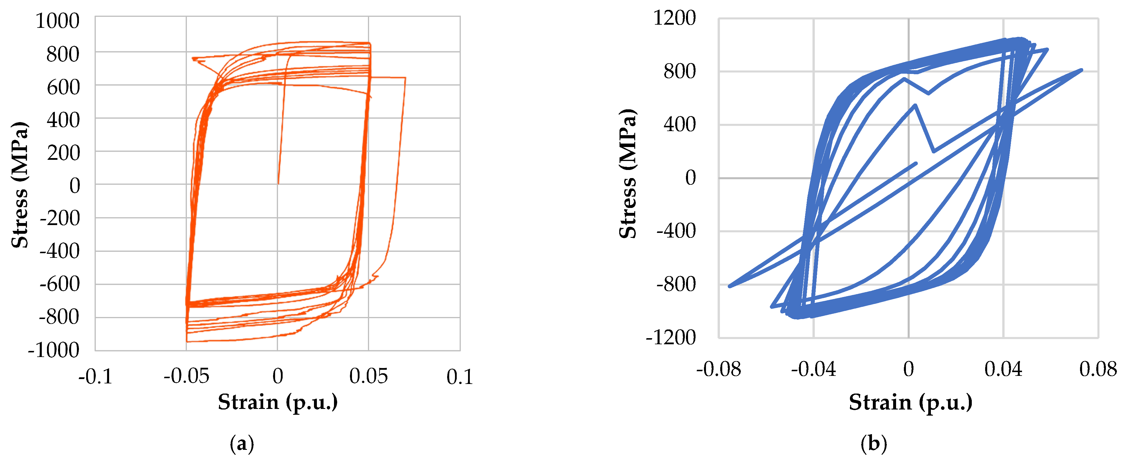
The hysteresis loops of the second S690 specimen generated for a total strain amplitude of ±0.07 p.u. are shown in Figure 11. The loops in Figure 11a are experimental and were taken from [26]. The loops in Figure 11b are numerical and were obtained in SIMULIA Abaqus 6.11 [22]. The results in Figure 11a,b correspond with eight and nine cycles to failure, respectively.

The conditions under which the hysteresis loops in Figure 11a were generated are as follows [26]: (1) non-sway buckling occurred in the first four half-cycles; (2) sway buckling occurred in the fifth half-cycle; (3) the number of cycles to failure was 8; and (4) the maximum stress recorded was 894 MPa. The maximum stress in the third quadrant was −1031 MPa. There also was one jump beyond the given limits of the total strain amplitude. The simulated result in Figure 11b refers to the test described. The differences between the experimental and simulated hysteresis loops are obvious. In this regard, the maximum stress values go up to approximately ±1115 MPa, and there are some jumps beyond the limits of the total strain amplitude.

Figure 12 describes the simulation of the cyclic loading history for the second S690 specimen, whose hysteresis loops are given in Figure 11b.

Based on the plots in Figure 12, the hysteresis curve in Figure 11b was generated by loading the second S690 specimen in nine cycles, each lasting 4 s. Failure of this specimen occurred at the beginning of the ninth cycle at a ULCF damage of 0.98.

A simulated ULCF behavior of the third S690 specimen at ±0.0074 p.u. of total strain amplitude is shown in Figure 13a. In addition to this, Figure 13b shows a comparison between the experimental and simulated data on the maximum stress versus the number of cycles to failure for two similar strain amplitudes. Specifically, the experimental data are taken from [28] and correspond with a total strain amplitude of ±0.01 p.u., while the simulated data correspond with a total strain amplitude of ±0.0074 p.u.

A hysteretic response similar to that in Figure 13a, obtained for a total strain amplitude of 0.01 p.u., can be found in [28]. Comparing the simulated responses in Figure 13a and Reference [28], a significant difference between the hysteresis loops can be observed in terms of their shapes, but almost identical maximum stress values were obtained for various numbers of cycles to failure, regardless of the difference between the total strain amplitudes of 0.0026 p.u. Moreover, it was not possible in SIMULIA Abaqus 6.11 to generate any hysteresis response for a total strain amplitude exactly equal to 0.01 p.u. Based on this, the comparison in Figure 13b was alternatively used to validate the model proposed here. Finally, it is evident that the data simulated using the proposed model correspond quite well with the available experimental data.

In the simulations of the initial loading cycles, the total strain amplitude was less than or approximately equal to ±0.05 p.u. (Figure 3b and Figure 9b) because the material under consideration was deformed to a lesser extent. With the simulation of each subsequent loading cycle, the material was more and more deformed, and the total strain amplitude gradually exceeded the value of ±0.05 p.u. This phenomenon was originally illustrated in Figure 2. Moreover, the same occurred when the total strain amplitude was ±0.07 p.u. (Figure 5b and Figure 11b), regardless of the material from which the tested specimen was made. Each FEA-based simulation lasted about 8 h. Therefore, the main reason for the deviation of the simulated hysteresis loops from the experimental ones were the conditions specified in the model. These conditions directly affected the establishment of stabilized states during the simulations of the ULCF behaviors of the considered specimens. Specifically, in these simulations, the number of cycles to failure was low, and the model itself tended to reach a stabilized hysteretic response after six or seven cycles. At lower total strain amplitudes, this negative phenomenon was not particularly pronounced. This can be seen in the plots in Figure 13, which were generated for a total strain amplitude of ±0.0074 p.u.

Figure 14 shows the plots of damage initiation, while Figure 15 shows the plots of damage evolution. The plots in both figures are generated for 90 cycles and five different stress ratios (namely, $R=-0.5$, $R=-0.6$, $R=-0.65$, $R=-0.7$, and $R=-0.73$).

According to Figure 14, material damage initiation significantly depends on the stress ratio $R$, which is defined as the quotient of the minimum and maximum stress values. In particular, as the mean stress (which is defined as the mean between the minimum and maximum stresses) decreases, material damage occurs much faster. From Figure 14, it can also be observed that the increase in maximum stress occurs with a gradual change in the stress ratio $R$ from −0.5 to −0.73. This change is accompanied by faster material damage initiation and lower total material degradation in the form of stress drop. The purpose of the stress plots in Figure 14 is to illustrate the behavior of the considered cylindrical bar for different stress ratios and different damage parameters obtained by the application of perfect axial cyclic loading.

Finally, from Figure 15, it is evident that the increase in the mean stress leads to a reduction in total damage and a delay in the initiation of material damage. In other words, with an increase in the tensile stress magnitude in relation to the pressure, there is an increase in the resistance of the material to the initiation and evolution of damage.

5. Conclusions

Based on the available experimental data, the values of damage parameters and the safety of real structures made of S355 and S690 steels for various cyclic loadings were assessed using finite element analysis. A simple, fast, and convenient approach to modeling material damage was demonstrated. The material damage growth over cycles was successfully monitored via a scalar damage variable. In the process of determining the material damage initiation and evolution parameters, the algorithm used gave results that agree well with those obtained using Kliman’s model for the hysteresis energy of cyclic loading.

Damage initiation under ultra-low-cycle fatigue conditions was determined based on the assumptions that plastic strains are equal to or greater than 0.025 p.u. and that damage appears already after the first loading cycle. It was found that the damage parameters $c_2$ and $c_4$ are material constants and that the values of the damage parameters $c_1$ and $c_3$ depend on the size of the finite elements and the system of units used in the model. More specifically, it was noticed that the parameter $c_4$ behaves as a material constant regardless of the condition of strain-controlled ultra-low-cycle fatigue. In addition, it was found that the damage initiation parameters $c_1$ and $c_2$ are 5.0 and −0.8, respectively.

Moreover, it was established that specifying values for the damage initiation parameter $c_1$ that are greater than 5.0 cannot affect damage initiation itself. Furthermore, it was shown that the damage initiation parameters $c_1$ and $c_2$ do not affect the damage evolution parameters $c_3$ and $c_4$. It was also shown that the evolution of damage in the considered materials takes place progressively for each cycle individually, the parameter $c_3$ contributes the most to this, and the parameter $c_4$ represents the fracture toughness of the materials. For lower amplitudes of cyclic loading, it was found that the correction of the parameter $c_3$ should be performed according to Equation (11) and the specified values for the coefficient $K$ and the exponent $n$. Finally, it was confirmed that the damage evolution parameters affect the shape and generation of hysteresis loops.

It was also concluded that in the case of direct cyclic analysis of real structures, there are the following limitations: (1) the concept of geometric linearity; (2) fixed connections between structural elements; (3) direct dependence of the accuracy and computational time of the applied method combining both iterative and incremental procedures on the input data; and (4) uniform growth of damage over cycles for strain amplitudes less than ±0.05 p.u.

Future research will focus on typical application scenarios for structural steels of the types S355 and S690 in seismic structures, the calibration of material damage parameters for other types of structural steels, and a comparative analysis of the results obtained using the direct cyclic algorithm and other applicable models. In addition, the implementation of some FEA-based models that would include the reality, that is, the nonlinearity of material damage evolution, could also be considered.