Article

Multi-Ship Collision Avoidance in Inland Waterways Using Actor–Critic Learning with Intrinsic and Extrinsic Rewards

1
College of Metropolitan Transportation, Beijing University of Technology, Beijing 100124, China
2
School of Automation, Chongqing University, Chongqing 404100, China
*
Author to whom correspondence should be addressed.
Symmetry 2025, 17(4), 613; https://doi.org/10.3390/sym17040613
Submission received: 13 March 2025 / Revised: 5 April 2025 / Accepted: 10 April 2025 / Published: 18 April 2025
(This article belongs to the Section Engineering and Materials)

Abstract

:
Inland waterway navigation involves complex traffic conditions with frequent multi-ship encounters. Benefiting from its straightforward structure and robust adaptability, reinforcement learning has found applications in navigation. This article proposes a deep actor–critic collision avoidance model which is based on the weighted summation of intrinsic reward and extrinsic reward, overcoming the sparsity of the reward function in navigation tasks. For the proposed algorithm, the extrinsic reward considers factors of collision risk, economic reward, and penalties for violating collision avoidance rules, while the intrinsic reward explores the novelty of agent states. The optimization of the own ship’s actions is achieved through the utilization of a weighted summation of these two types of rewards, providing valuable guidance for decision-making in a symmetrical interaction framework. To validate the performance of the proposed multi-ship collision avoidance model, simulations of both two-ship encounters and complex multi-ship scenarios involving dynamic and static obstacles are conducted. The following conclusions can be drawn: (1) The proposed model could provide effective decisions for ship navigation in inland waterways, maintaining symmetrical coordination between vessels. (2) The hybrid reward mechanism successfully guides ship behavior in collision avoidance scenarios.

1. Introduction

Inland water transportation refers to a type of transport which uses ships to transport goods and passengers through natural or artificial waterways. By the end of 2021, China’s inland waterway navigation mileage had surpassed 127,700 km [1]. As a crucial component of the water transportation network, inland navigation is essential to the national economy. However, the growing traffic on these waterways has also resulted in an increase in ship safety incidents [2,3]. The statistics show that ship collisions account for the majority of all types of accidents. Therefore, the analysis of collision avoidance for inland transportation has become the focus of inland navigation. Numerous ship collision avoidance methods have been explored in research, which can be categorized into two main types: traditional methods and intelligent methods [4,5].

1.1. Traditional Approaches

Traditional methods include path generation, the synthetic indicator approach, the safety boundary algorithm, and the velocity-based approach. For path generation, Ref. [6] explores an A* method, which takes an enclosed circular boundary as a safety constraint to generate the motion planning for vessels moving in a maritime environment. The local path generation method, such as the potential field approach, has been verified to be effective to avoiding stationary obstacles in research [7]. This algorithm has a faster computational speed than the heuristic A* search algorithm [8]. Hierarchical planning and more constraints are used to search for smoother paths, which can improve the efficiency as well compared with A* [9]. For synthetic indicator approaches, parameters reflecting the relationships between ships can be selected to be the criteria of tasks. Kouzuki et al. identified DCPA (distance to the closest point) and TCPA (time to the closest point) as indicators of collision risk, which are used to determine the ship’s steering actions for avoiding collisions [10]. The collision risk level can be detected using indicators, and then the movement of ships (such as speed, course, etc.) can be calculated when they encounter static and dynamic obstacles [11]. The evidential reasoning theory integrating the COLREG guidelines is proposed to evaluate the collision risks in encounter situations [12]. In reality, the understanding of collision risk level would vary with the different indicators which reflect the spatio-temporal relationships between ships and obstacles [13]. From another perspective, Degre et al. proposed that velocity-based methods can analyze ship collision problems, such as the velocity obstacle algorithm [14]. As an improved velocity method, the generalized velocity obstacle algorithm can overcome the assumptions in other studies, such as constant velocity and simplification of ship’s dynamics [15,16]. The counteraction navigation algorithm seeks to enhance the misalignment between the relative velocity and the line of sight by utilizing the ships’ acceleration [17]. In ref [18], the safe velocity space for multiple ships in the encountering situation is defined in the related algorithms, whose basic concept is to find the available room for maneuver.
There are also many scholars focusing on the research of safe boundary approaches which have been evolving with time [19,20,21]. Hara provided an empirical method called the bumper model to detect the safe area around the ship, as shown in Figure 1 [22]. The shape can be described by a half ellipse and half circle, with the two parameters L 1 = 6.4 L and L 2 = 1.6 L , and L represents the length of the ship.
Regarding the different encounter situations, Coldwell et al. proposed a definition of the ship domain (expressed in multiples of ship length, L), which indicates the safe space around the ship, as shown in Figure 2 [23]. The ship domain refers to the area that should be kept clear; otherwise, there will be a risk of collision.

1.2. Intelligent Methodologies

With the development of intelligent algorithms, more and more scholars have paid attention to optimization-based methods [24,25]. The evolutionary algorithms and fuzzy logic are examined in the area of autonomous collision avoidance [26]. The Ant Colony Algorithm is combined with navigational practices to construct a hybrid model to plan a safe and economy path in advance [27]. A symmetric role-classification criterion is employed to enhance traffic rules, while the probabilistic velocity method is utilized to prevent potential collisions. The effectiveness of this approach is validated through Monte Carlo simulations of multi-ship encounter scenarios [28]. A dynamic path planning algorithm combining A* and navigation rules is proposed, and the search mechanism considers the time factor in the situations with moving obstacles [29]. The beam search algorithm is taken into consideration to choose the best moving path based on the length and other criteria. The risk of collision of ship is determined based on the nearest point of approach [30]. The danger immune algorithm aims to find a set of optimal operation instructions for ships to realize reliable collision avoidance while obeying COLREG [31].
Recently, reinforcement learning has also been adopted to address these problems. Deep reinforcement learning is used for ship collision avoidance, in which the obstacle zone by target can reflect the safe area around the ship [32]. The actor–critic deep reinforcement learning framework is commonly used in ship collision avoidance. In reference [33], the actor network determines appropriate rudder angles based on real-time ship states and collision risk assessments, while considering both COLREGs compliance and path optimization in open sea. A collision map is employed as input state representation and self-adaptive parameter sharing between critic and actor networks is introduced to improve training convergence, effectively handling complex maritime scenarios in busy ports [34]. The actor–critic variant is combined with LSTM and Q-learning to create a composite learning framework for ship collision avoidance, where Q-learning adaptively switches between LSTM-based control and A3C policies to improve the efficiency of the model [35]. A variant of actor–critic is employed for ship collision avoidance with dual-mode operation (path-tracking and collision avoidance), where the system generates COLREG-compliant continuous actions based on encounter identification and risk assessment [36]. Proximal policy optimization is used within a partially observable Markov decision process for ship collision avoidance in mixed-obstacle environments, where image-based state observations and dense reward functions are used to improve decision-making accuracy [37]. This study optimizes the parameter update and exploration strategies of actor–critic algorithms to improve ship obstacle avoidance performance in complex offshore environments [38] More information and navigation rules should be taken into consideration, such as channel environment and rules which are related to the narrow channel navigation [39,40].
The navigation conditions in inland waterways are complex, and collision accidents often occur in narrow channels due to the heavy traffic and limited movements. This paper introduces a multi-ship collision avoidance system based on deep reinforcement learning which maintains symmetrical coordination between vessels. Symmetrical coordination refers to a balanced collision avoidance framework where all vessels have equal decision-making priority except when navigation rules specify otherwise. This means each vessel makes decisions by considering both its own safety and the maneuverability of other vessels. The proposed method incorporates both extrinsic and intrinsic rewards to address the issue of reward function sparsity in navigation tasks. The extrinsic reward evaluates collision risk, economic efficiency, and rule compliance, while the intrinsic reward explores state novelty in the ship’s decision space. Ship navigation decisions are optimized through a weighted combination of these rewards. The model’s effectiveness is validated through simulations of both typical two-ship encounters and complex scenarios involving multiple moving and stationary obstacles.

2. Preliminaries

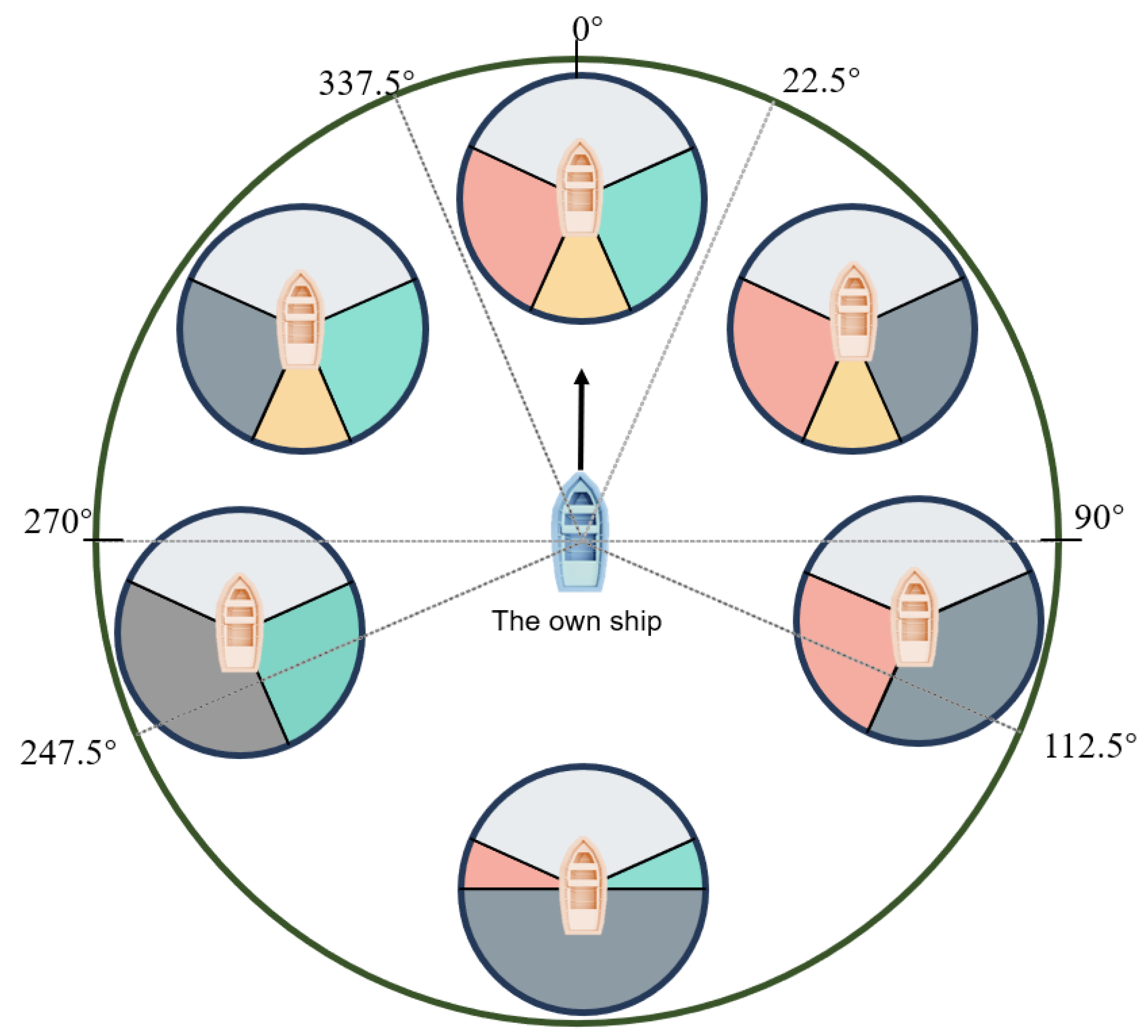
2.1. Ship Encounter Situations

Inland waterways present unique navigational challenges due to natural obstacles and channel limitations. This study classifies vessel encounters into five categories based on relative bearing and course: head-on, overtaking, starboard crossing, port crossing, and safe situations, as shown in Figure 3 [41]. According to the rules of Inland Waterway Regulations for Preventing Collisions (IWRPC), there are some situations that should be addressed.
  • The vessels should stay as close to the outer limit of the channel on their starboard side as is safe and practical (rule 8).
  • Under any circumstances, ferries navigating the main channel of the Yangtze River must yield to vessels traveling downstream or navigating the channel (rule 9).
  • Crossing vessels must yield to vessels traveling downstream or navigating the channel and must not suddenly or forcefully cross in front of vessels that are proceeding downstream (rule 12).
  • In a head-on situation (two power-driven vessels are meeting on reciprocal or nearly reciprocal courses) with a risk of collision, both vessels should turn to starboard to pass port side to port side (rule 10).
  • If one vessel plans to overtake another one, in which the vessel approaches another vessel from a direction more than 22.5 degrees abaft the beam, it must not impede the movement of the vessel being overtaken (rule 11).
  • When two vessels are crossing and a collision risk exists, the vessel with the other on its starboard side should give way and avoid crossing ahead of the other vessel (rule 12).

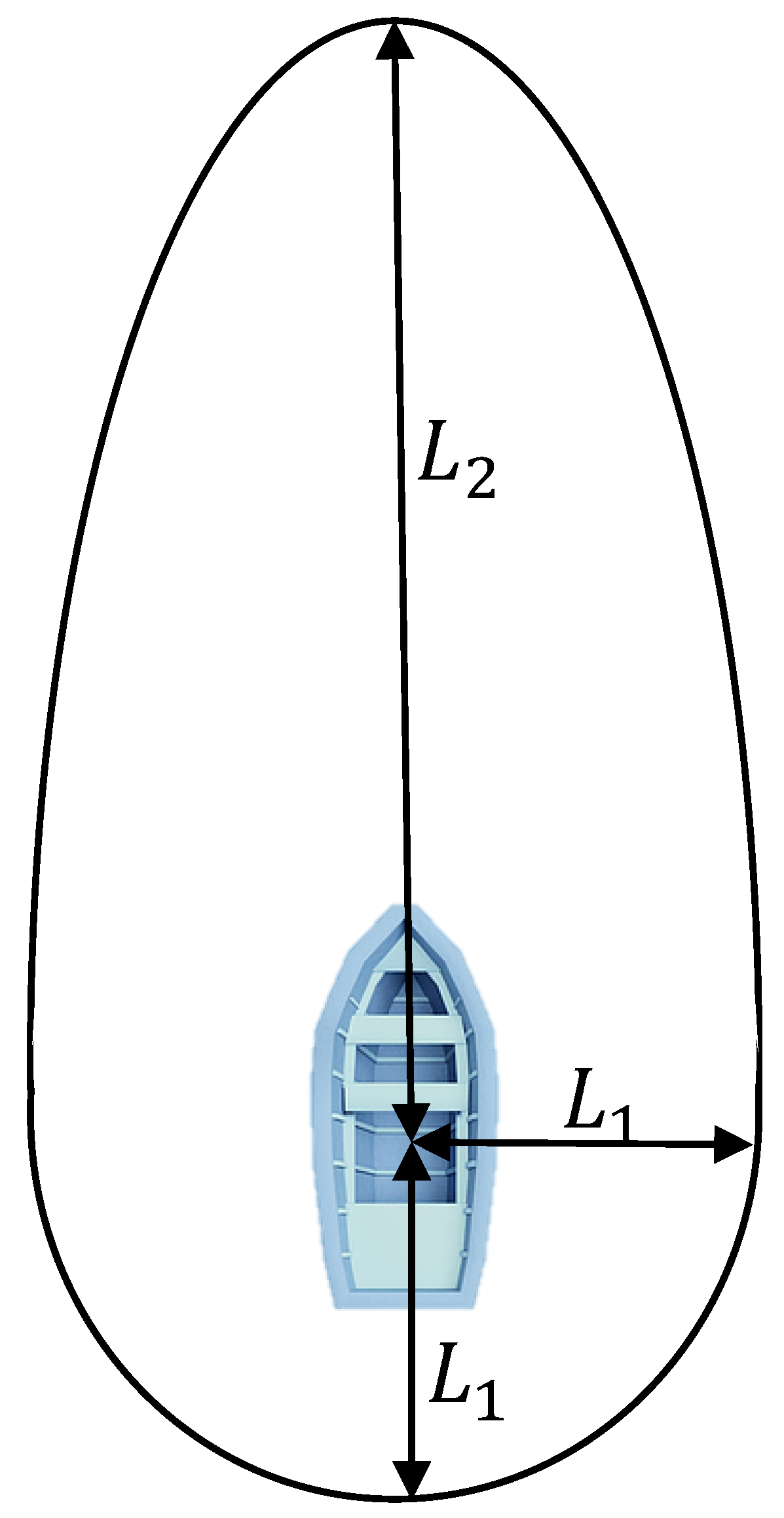
2.2. Collision Diameter

The concept of collision diameter (CD) is proposed to define the minimum area around the ship necessary to prevent collisions, which is firstly defined as the proportion of the lengths of ships [42]. The area defined by the CD represents a zone where no collision has occurred. However, an obstacle ship entering this zone is at risk of collision. This research mainly focuses on collision avoidance in restricted waterways where the speed of ships should also be taken into consideration in different encounter scenarios, as shown in Figure 4. This paper adopts an improvement in collision diameter to describe the safe area of the ship [43], as shown in Equation (1), where the waterline area of the ship is approximated by a rectangular shape.
D i j = L i V j + L j V i V i j sin θ + B j [ 1 ( sin θ V i V i j ) 2 ] 1 / 2 + B i [ 1 ( sin θ V j V i j ) 2 ] 1 / 2
where D i j is the collision diameter of vessels in i-th and j-th waterways; L i and L j are the lengths of ship i and ship j; B i and B j are the widths of ship i and ship j; V i and V j are the speeds of ship i and ship j; V i j is the relative speed of ship i and ship j; θ is the relative bearing of two ships, which should be limited to an interval at different encountering situations for practical reasons [44]:
Taking-over ( θ = 0 10 );
Crossing ( 10 < | θ | < 170 );
Head-on ( θ = 180 ± 10 ).
Figure 4. The definition of collision diameter D i j .
Symmetry 17 00613 g004
In situations of take-over or head-on encounters, the meeting angle θ in Equation (1) is presumed to be 0 or 180 degrees, respectively, and the collision diameter corresponds to the combined width of both ships. For the crossing encounters, Equation (1) applies with the given θ value. Equation (1) can be rewritten as an alternative representation of Pedersen’s original equation [45,46]:
D i j = L i sin α + L j sin β + B i cos β + B j cos α
For better understanding and simplification, Equation (2) is adopted in this article.

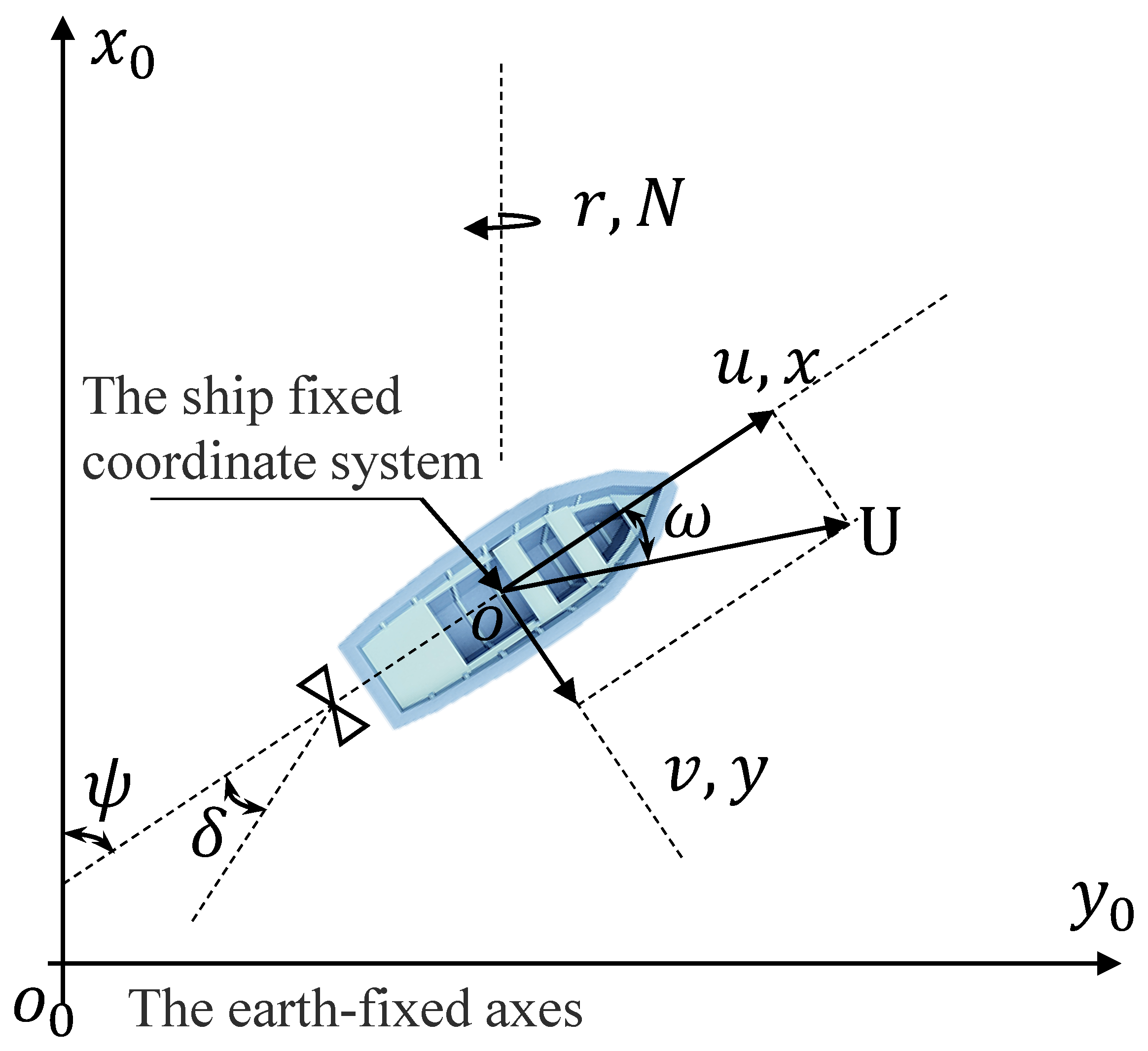
2.3. Ship Motion Model with Environmental Disturbances

There are nonlinear characteristics and hysteresis in the maneuvering motion of ships. The mathematic model, known as the maneuvering modeling group, is commonly utilized to articulate the process for ship motion modeling [47,48].
Typically, the ship motion coordinate system is depicted in Figure 5. The earth-fixed coordinate system is represented as o 0 - x 0 y 0 z 0 , with the x 0 - y 0 plane aligned with the still water surface and the z 0 axis pointing vertically downward. The moving ship’s coordinate system is o- x y z , where o is located at the ship’s midpoint, where the x axis points towards the bow, the y axis towards the starboard, and the z axis vertically downwards. For simplicity in accommodating various load conditions such as full or ballast load, this paper assumes the ship’s center of gravity is located at the mid-ship position. The environmental disturbances significantly influence ship maneuverability, particularly in inland waterways where channel constraints limit the available space for navigation. In this article, the ship motion model can be extended to incorporate environmental disturbances such as wind, current, and waves:
( m + m x ) u ˙ ( m + m y ) v r = X H + X R + X P ( m + m x ) v ˙ ( m + m x ) v r = Y H + Y R ( I z z + J z z ) r ˙ = Y H + N R
where the subscripts H, P, and R denote the hull, propeller, and rudder, respectively. Additionally, m denotes the ship’s mass, m x and m y denote the added mass in the x and y directions, I z z denotes the moment of inertia, J z z denotes the polar moment of inertia, u represents the surge velocity, v represents the sway velocity, and r denotes the yaw rate.
The hydrodynamic forces and moments exerted on the hull can be represented in the following manner:
X H = 1 2 ρ L d U 2 [ X u u ( 0 ) + X b b b 2 + X b r b r + X r r r 2 + X b b b b b 4 ] Y H = 1 2 ρ L d U 2 [ Y b b + Y r r + Y b b b b 3 + Y r r r r 3 + ( Y b b r b + Y b b r r ) b r ] N H = 1 2 ρ L 2 d U 2 [ N b b + N r r + N b b b b 3 + N r r r r 3 + ( N b b r b + N b b r r ) b r ]
where b is the drift angle and r is the dimensionless turning rate, which are expressed as b = s i n ( v / U ) and r = r ( L / U ) . The formula for the force and moment produced by the propeller revolution n is expressed as follows:
X P = ρ D p 4 n 2 ( 1 t ) K T
Taking the interactions between hull and rudder into account, the force and moment induced by rudder δ can be expressed as follows:
X R = ( 1 t R ) F N sin ( δ ) Y R = ( 1 + a H ) F N cos ( δ ) N R = ( x R + a H x H ) F N cos ( δ )

3. Multi-Agent Reinforcement Learning for Collision Avoidance

3.1. Grid Mesh Discretization

The collision diameter needs to be detected with high resolution over a wide area spanning several nautical miles. According to collision avoidance rules, actions to prevent a collision must be decisive and taken promptly. Observing the situation from a sufficient distance is crucial to select an appropriate action in a timely manner. Therefore, the area surrounding the own ship is divided into a grid extending from the ship’s center, with evenly spaced intervals in both the angular and radial directions, forming a concentric circle grid. When a grid cell intersects with the boundary of the collision diameter, its state is set to 1; otherwise, it is set to 0. This creates a state vector that can represent the risk area around the own ship.
The action space for the own ship in various encounter scenarios includes all possible collision avoidance maneuvers. Examples include turning to port, turning to starboard, accelerating, and decelerating. To reduce computational load and improve training efficiency, the action space is discretized. Using 5 as the minimum steering angle, the ship turns to port or starboard are distributed between [ 60 , 60 ] to prevent collision risks from continuous small-angle adjustments. Additionally, actions to maintain the current course and speed are considered.

3.2. Definitions of Collision Avoidance Model
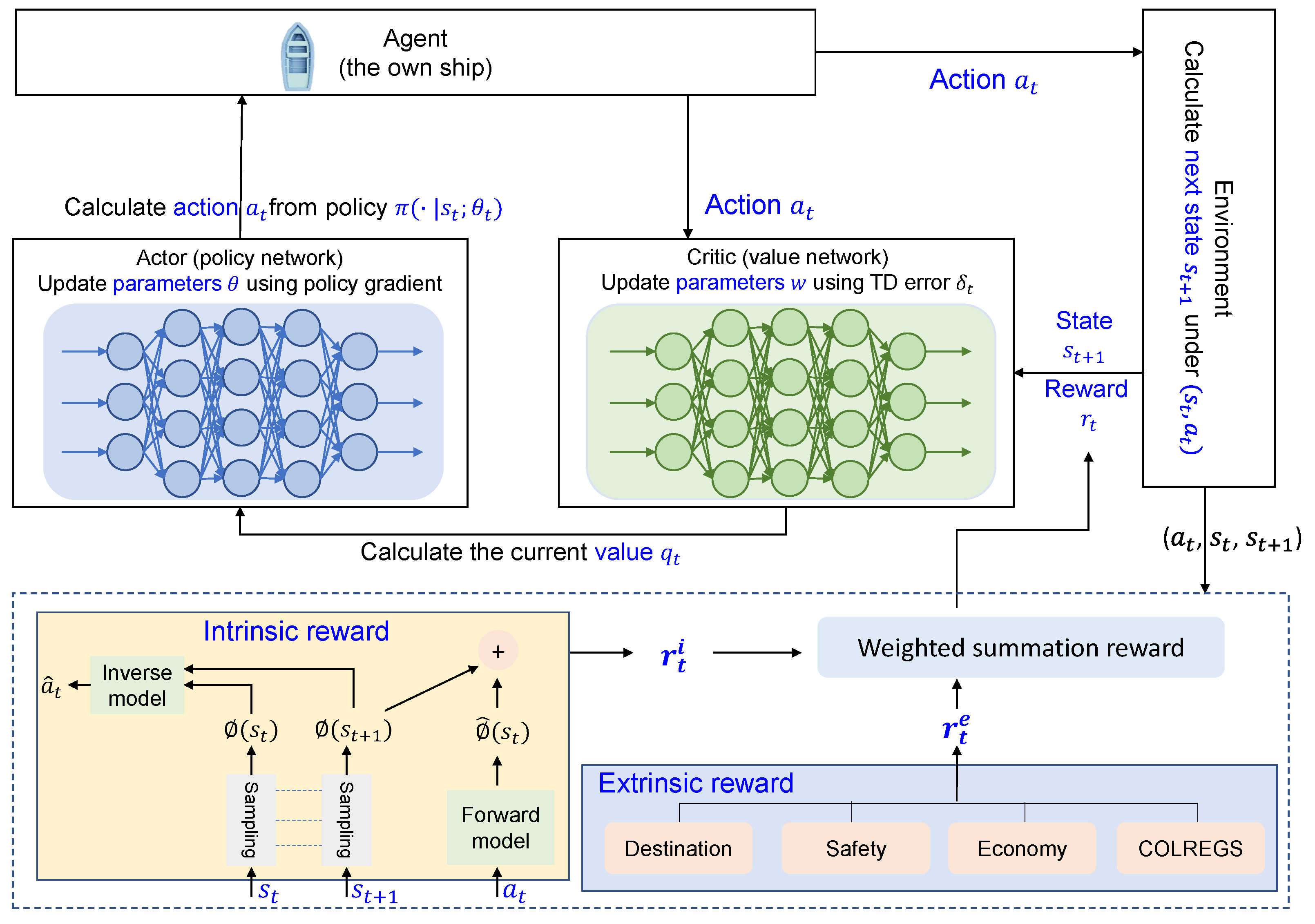
The collision avoidance problem is a maximin problem, which involves maximizing, with respect to the state and control of the maneuvering ship, the minimum distance between the two ships over time [49]. The goal of ship collision avoidance is to reach the destination without colliding with any obstacle ships. Therefore, the performance of collision avoidance model may be compromised when there is incomplete information about other ships, such as positions or velocities. As shown in Figure 6, the information the ship observes from the environment at time step t is defined. The state of the own ship can be described as follows: s o t = [ x o t , y o t , v o t , φ o t , δ o t , n o t , d d t ] , where [ x o t , y o t ] represents the position of the own ship; v o t is the speed of the own ship; φ o t is the course of the own ship; δ o t is the rudder angle of the own ship; n 0 t is the propeller rotation speed of the own ship; d d t represents the distance between the own ship and the destination at time step t, which can be calculated by the following:
d g t = ( x o t x d ) 2 + ( y o t y d ) 2
where [ x d , y d ] is the destination of the own ship. The state of the i-th obstacle ship at step t can be defined as follows: s i t = [ x i t , y i t , v i t , δ i t , n i t , α i o t , d i o t ] , where [ x i t , y i t ] is the position of the i-th ship; v i t is the velocity of the i-th ship; δ i t is the rudder angle of the i-th ship; n i t is propeller rotation speed of the i-th ship; α i o t and d i o t denote the relative angle and distance from the own ship to the obstacle ship at step t, respectively.
d i o t = ( x i t x o t ) 2 + ( y i t y o t ) 2
α i o t = arctan Δ y t Δ x t ψ o t x i t x o t ;   y i t y o t π + arctan Δ y t Δ x t ψ o t x i t x o t ;   x i t x o t x i t < x o t ;   y i t y o t 2 π + arctan Δ y t Δ x t ψ o t x i t < x o t ;   y i t > y o t
where Δ y t = y i t y 0 t , Δ x t = x i t x 0 t .

3.3. Reward Design

In the navigation task, the reward could only be achieved when the own ship reaches the destination, which leads to a sparse reward function in reinforcement learning. During the early stage of the training process, if the own ship cannot receive feedback from the reward function most of the time, the decision policy would become random. While if the own ship is navigated based on a series of random decisions and actions, the probability of reaching the destination becomes extremely low.
In reality, this inefficient exploration method would not be allowed due to energy and safety considerations. Intrinsic rewards in deep actor–critic models are often used to encourage exploration of the environment. This helps the agent discover new states and actions that may not be explored through extrinsic rewards alone. By incorporating intrinsic rewards, the reward function would become denser at the early training stage. At the same time, extrinsic rewards are typically defined by the external environment, such as achieving a goal or maximizing a performance metric. These rewards guide the agent toward achieving predefined objectives. To expedite the model’s convergence rate and direct the own ship towards making informed decisions for collision avoidance, this article proposes a weighted function of intrinsic reward which can explore the state novelty of the own ship and extrinsic reward which considers feedback from the environment.
The effectiveness of our approach depends significantly on the appropriate weighting of different reward components. Therefore, the overall reward function combines intrinsic and extrinsic components as defined:
r t = w i · r t i + w e · r t e
where r t i is the intrinsic reward based on state novelty, and r t e is the extrinsic reward considering safety, economy, and rule compliance; w i and w e are weighting factors for intrinsic and extrinsic rewards, respectively.

3.3.1. Intrinsic Reward

By providing intrinsic rewards for novel actions or states, agents can explore their environments more thoroughly, leading to better policy development. Moreover, agents can become more robust to variations in the environment since they are not solely reliant on extrinsic rewards, which may be sparse or misleading.
The state novelty is explored through a sophisticated intrinsic reward mechanism that significantly differs from traditional exploration strategies. While conventional methods typically rely on random action selection or simple probability distributions, our approach implements a dynamic novelty-driven exploration strategy.
In order to come up with a good intrinsic reward signal, this article introduces a deep neural network comprising two modules: the initial module encodes the raw state s t into a feature vector ϕ ( s t ) , and the subsequent submodule utilizes the feature encodings, ϕ ( s t ) and ϕ ( s t + 1 ) , of two consecutive states as inputs to forecast the action a t performed by the agent to transition from state s t to s ( t + 1 ) . Training this neural network involves learning the function g, as defined by
a ^ t = g ( s t , s t + 1 ; θ t )
where g is the inverse dynamic model, a ^ t is the prediction of a t , and θ I are optimized by minimizing
min θ I L I ( a ^ t , a t )
where L I represents the loss function, which quantifies the difference between the actual action and the predicted action.
For the forward dynamic model, this article trains a separate neural network that accepts a t and ϕ ( s t ) as inputs and predicts the feature encoding of the state at the subsequent time step t + 1 ,
ϕ ^ ( s t + 1 ) = f ( a t , ϕ ( s t ) ; θ F )
where ϕ ^ ( s t + 1 ) is the predicted estimate, and the parameters θ F are refined through minimizing the loss function L F :
L F ( ϕ ( s t + 1 ) , ϕ ^ ( s t + 1 ) ) = 1 2 | | ϕ ^ ( s t + 1 ) ϕ ( s t + 1 ) | | 2 2
Therefore, the intrinsic reward is computed as
r t i = η 0 2 | | ϕ ^ ( s t + 1 ) ϕ ( s t + 1 ) | | 2 2 + η 1 N ( s )
where η 0 and η 1 are scaling factors; N ( s ) is the state novelty score:
N ( s ) = 1 / ( 1 + V ( s ) )
where V ( s ) is the number of times state s has been visited.

3.3.2. Extrinsic Reward

Extrinsic rewards provide clear and measurable goals for the agent, guiding its learning process toward specific outcomes. In addition, agents can converge more quickly to optimal policies with well-defined extrinsic rewards. In this article, the extrinsic reward function for collision avoidance is crafted considering safety and economic factors. It encompasses rewards for reaching the destination, penalties for collisions, penalties for encroaching on another ship’s domain, and penalties for straying from the designated route. In this article, the extrinsic reward can be expressed as follows:
r t e = w d · r t d + w s · r t s + w m · r t m + w c · r t c
where w d , w s , w m , and w c are the weights for destination, safety, economy, and rule compliance rewards, respectively.
Destination reward: The r t d is constructed to guide the own ship to arrive at the destination or point as soon as possible. It can be expressed by the equation:
r t d = K 1 ( | P t o P d | | P t 1 o P d | ) K 2 if | | P t o P d | | < ε
where r t d is related to the distance to the destination at t and t 1 ; K 1 and K 2 are scaling parameters; P t o and P d are the positions of the own ship at step t and at the destination, respectively; ε is a threshold value. When the ship reaches a certain range around the destination, it is considered that the ship has successfully completed the journey.
Collision reward: To assess the risk of ship collision, classical ship domains serve as limits to determine the presence of collision risk. More precisely, if an obstacle ship is situated beyond the boundaries of the own ship’s domain, there is no risk of collision; however, if it falls within those boundaries, the risk of collision exists [50]. The probabilistic ship domain not only evaluates the likelihood of collision but also measures the level of risk based on probability. In multi-ship scenario, when the own ship focuses on a specific obstacle ship and makes decisions, the distance separating the own vessel from the i-th obstacle vessel may temporarily fall below D o i temporarily. While this state may not result in a collision, it poses a threat to navigation safety. Hence, the collision risk can be assessed based on the frequency of distances smaller than the safe distance between ships. The reward of safety can be defined by the formula of ship collision risk [51]:
r t s 1 = 1 0 < d D o i ( 1 0 d D o i f θ ( ω ) d ω ) D o i < d L
where d represents the distance to the own ship. The domain probability function f θ ( ω ) is defined by the probability density function δ ( θ ) , derived from the distribution of obstacle ships at various distances, which can be obtained from historical ship trajectories. D o i marks the boundary of the own ship’s safety zone.
Furthermore, we compute the acceleration and deceleration for each successive vessel record individually [52]:
a i , t = v i , t v i , t k k
where a i , t represents ship i’s acceleration over ground at time t, and v i , t and v i , t k represent the ship i’s speed over ground at time ( t k ) . In this research, we calculate the average of the squared values of acceleration and deceleration as an additional collision risk indicator:
r t s 1 = i = 1 I t = 1 T a i , t 2 I
where r t s 1 is the degree of acceleration and deceleration; I represents the count of vessel i records within the vicinity of L around the own ship.
Therefore, the reward of safety is as follows:
r t s = λ s 1 r t s 1 + λ s 1 r t s 2
Economy reward: During the voyage, steering with a substantial rudder angle leads to a reduction in the ship’s surge speed and an extension of the sailing time. Generally, economic incentive can be reflected by the energy loss resulting from large rudder angles and propeller revolution:
r t m 1 = γ 1 δ i , t δ i , t k k + γ 2 n i , t n i , t k k
Furthermore, it is crucial for the own ship to prevent significant deviations from its initial paths. Therefore, this study employs the commonly used line-of-sight (LOS) guidance strategy. Figure 7 depicts the LOS guidance method as the own ship moves between adjacent path nodes, P k ( x k , y k ) and P k + 1 ( x k + 1 , y k + 1 ) . The current heading angle and position of the own ship are denoted as ψ and P ( x , y ) , respectively.
In the LOS guidance method, the ship is directed by reducing the difference between its current heading angle and the LOS angle. The LOS angle is calculated by solving the following set of equations:
( x L x ) 2 + ( y L y ) 2 = R L 2 y L y k x L x k = y k + 1 y k x k + 1 x k φ L = arcsin ( x L x R L )
where P L ( x L , y L ) represents the LOS guidance point, with R L being the radius of the acceptance circle, which can be defined as follows:
R L 1 = 3 L 1 , | e | 3 L 1 | e | + L 1 , | e | > 3 L 1
where e is the cross-tracking error and L 1 is the ship length.
Next, the square of LOS tracking error ( Δ φ ) 2 is employed to construct the economic reward related to re-sailing as follows:
r t m 2 = 1 2 ( Δ φ ) 2 = 1 2 ( φ L ψ ) 2
Then, the reward of economy can be calculated by the following:
r t m = λ m 1 r t m 1 + λ m 2 r t m 2
where λ m 1 and λ m 2 are the associated weights.
Rule compliance reward: According to the rules, the reward of rule constraint could be expressed as the following equation:
r t c = μ τ if meeting and taking collision risk 0 e l s e
where τ represents the penalty coefficients for breaching the regulations; μ indicates a 0–1 variable, which means whether the ships obey the rules. If μ is 0, this means the ships obey the rules; otherwise, it means they do not obey.

3.4. Actor–Critic Collision Avoidance Method

To develop a universal policy applicable to various obstacle ships, the process of avoiding collisions in multi-ship scenarios is enhanced through the actor–critic method of reinforcement learning. The detailed description is as follows: At time step t, the agent ship executes an action to prevent collisions and obtains a reward r t according to Equation (9).
The actor policy network which is formulated by the deep neural network is used to learn the collision avoidance strategy, in other words, the best action when the own ship meets obstacle ships. The actor policy network consists of an input layer that receives the environment state. It features two hidden layers: the first hidden layer comprises 128 nodes, while the second hidden layer has 64 nodes, both employing ReLU activation. The output layer produces a probability distribution over actions, using a softmax function for normalization. The parameters of the actor network include weight matrices and biases: the first hidden layer has a weight matrix W 1 R 128 × S and bias b 1 R 128 , the second hidden layer uses W 2 R 64 × 128 and b 2 R 64 , and the output layer employs W 3 R A × 64 and b 3 R A . The critic value network shares a similar architecture, starting with an input layer that also receives the environment state. It includes two hidden layers, with 128 and 64 nodes, respectively, both utilizing ReLU functions. The output layer provides a scalar value that represents the expected return for the current state, with no activation function applied. The critic’s parameters mirror those of the actor, featuring corresponding weight matrices and biases for each layer. The weight matrices for the first hidden layer are W 1 R 128 × S and bias b 1 R 128 , and for the second hidden layer, they are W 2 R 64 × 128 and b 2 R 64 . The output layer’s parameters are W 3 R 1 × 64 and b 3 R 1 . The formula of the actor–critic method could be expressed as follows:
J ( θ ) = E s 0 , a 0 , , s t , s t [ t = 0 T 1 θ log π θ ( a t | s t ) Q w ( s t , a t ) ] = E τ [ t = 0 T 1 θ log π θ ( a t | s t ) Q w ( s t , a t ) ]
where V w ( s t , a t ) represents the critic value network, and π θ ( a t | s t ) represents the actor policy network.
In the training process, the parameters of two networks are updated iteratively by gradient descent/ascent strategy. The pseudocode is shown in Table 1. The TD target of the critic network is based on the rewards. Considering the significant hysteresis in ship motion, the effect of the present rudder action on future rewards is considered. Therefore, we analyze the obtained discounted reward vector over a defined time horizon:
y t = R t + γ q ( t + 1 ) + γ H q ( t + H )
where H is the discounted horizon, [ γ , γ 2 , γ H ] is the discount vector, and q ( t ) is the output of critic network at step t. Thus, the TD error is δ t = ( q t y t ) 2 , which is used to update the critic value network.
Following the training process, the action strategies for the own ship in various obstacle ship scenarios are revised and consolidated from the actor network. The framework of the strategy for avoiding collisions among multiple ships is illustrated in Figure 8.

4. Experimental Data and Baseline Algorithms

In all the case studies, we implemented the networks using TensorFlow and performed tests on a four-core i5 CPU with eight threads. Dynamic environments, as well as scenarios involving the coexistence of dynamic and static environments, are established. Additionally, the effectiveness and rationality of avoidance actions are analyzed based on the closest avoidance distance and computational time.

4.1. AIS Dataset Characteristics

To evaluate the practical applicability of the proposed model, we extract Automatic Identification System (AIS) data. AIS provides real vessel information including position, course, speed, and vessel characteristics, enabling the validation of our model against actual navigational behaviors.
The AIS dataset used in this study is collected from the middle/lower reaches of the Yangtze River, with approximately 200 representative encounter scenarios. For validation, we extract several typical encounter scenarios from the AIS data, including head-on, crossing, and overtaking situations. These real-world scenarios serve as the baseline for evaluating the performance of the proposed model against the action taken by human operators in real world.

4.2. Comparable Algorithms

To evaluate the performance of the proposed actor–critic model with intrinsic and extrinsic rewards, we implement several state-of-the-art reinforcement learning algorithms and traditional collision avoidance methods as baselines. (1) Proximal policy optimization (PPO): A policy gradient method that uses an objective function to constrain policy updates, making learning more stable. (2) Asynchronous advantage actor–critic (A3C): A parallel implementation of the actor–critic algorithm that uses multiple agents to explore different parts of the environment. (3) Deep deterministic policy gradient (DDPG): An off-policy algorithm combining DQN and actor–critic approaches which uses deterministic policy gradients. (4) Velocity obstacle (VO): A traditional collision avoidance method that defines the set of velocities that would lead to collision with obstacles.
All algorithms are implemented with hyperparameter optimization to ensure fair comparison. For the reinforcement learning algorithms, we maintain identical neural network architectures and use the same state and action space definitions to isolate the effects of algorithmic differences.

5. Simulation Design

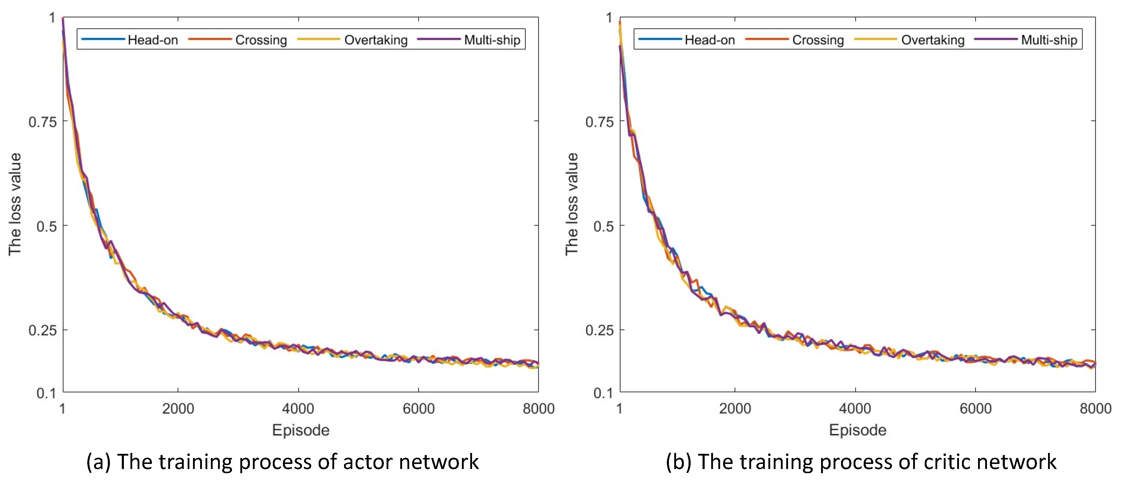
5.1. Training Process

In the section, a detailed description is proposed, including the training parameters and data utilized. In Table 2, the discount rate determines the importance of future rewards compared to immediate rewards, and the maximum episode implies the maximum number of iterations for learning. Max step means the maximum number of actions allowed within a single episode. Batch size is the number of samples used for network update during training. The learning rates of the actor and critic networks are the rates of updating each network.
In reinforcement learning, training data are dynamically generated through the interaction between the ships (agents) and environment, forming an iterative learning process. Through this process, ships develop collision avoidance behavioral strategies. During training process, mini-batches are randomly sampled to allow for diverse experiences to be used in updating the networks. The loss values for both the actor and critic networks are plotted over training episodes to visualize performance improvements in Figure 9. The learning curves of both actor and critic networks demonstrate similar and effective training patterns. Both networks start with high error rates (0.8–1.0) and show rapid initial improvement in the first 1000 epochs, followed by a gradual stabilization after epoch 2500.
As shown in Table 3, the convergence characteristics across typical collision avoidance scenarios are analyzed. For the four algorithms (A3C, PPO, DDPG, and Proposed model) tested across different ship collision avoidance scenarios, the proposed model demonstrates superior performance. It requires fewer episodes to converge, as well as lower actor and critic final losses (approximately 0.15–0.16 and 0.13–0.17, respectively). The multi-ship scenario presents the most challenging case for all algorithms, requiring more episodes and a longer convergence time, with DDPG consistently showing the slowest convergence. The training phase of the proposed model is conducted using high-performance computing resources. Each training episode consumed approximately 10 s, resulting in a total training duration of 22 h for all 8000 episodes. Once trained, the model demonstrates excellent real-time performance in practical applications, which will be discussed in the experimental results and analysis.

5.2. Parameter Settings

The coefficients of the ship motion model, known as hydrodynamic derivatives, can be obtained through model tests using scaled vessels [53]. Table 4 presents the values of these derivatives used in this experiment.
The simulations are conducted using vessel parameters typical of inland waterway cargo ships. Additionally, the simulation scenarios incorporate two types of obstacles: static and dynamic. Static obstacles represent waterway features such as channel boundaries and shallow water areas. Dynamic obstacles consist of other vessels with varying encounter situations.
Considering dynamic environmental changes, the proposed model implements a comprehensive real-time state update mechanism to ensure responsiveness to a dynamic environment. Environmental states are updated every 30 s, continuously monitoring and integrating obstacle vessel trajectories and environmental conditions. This integration enables the model to adapt its collision avoidance strategies according to changing environmental conditions, ensuring robust performance across various maritime scenarios.

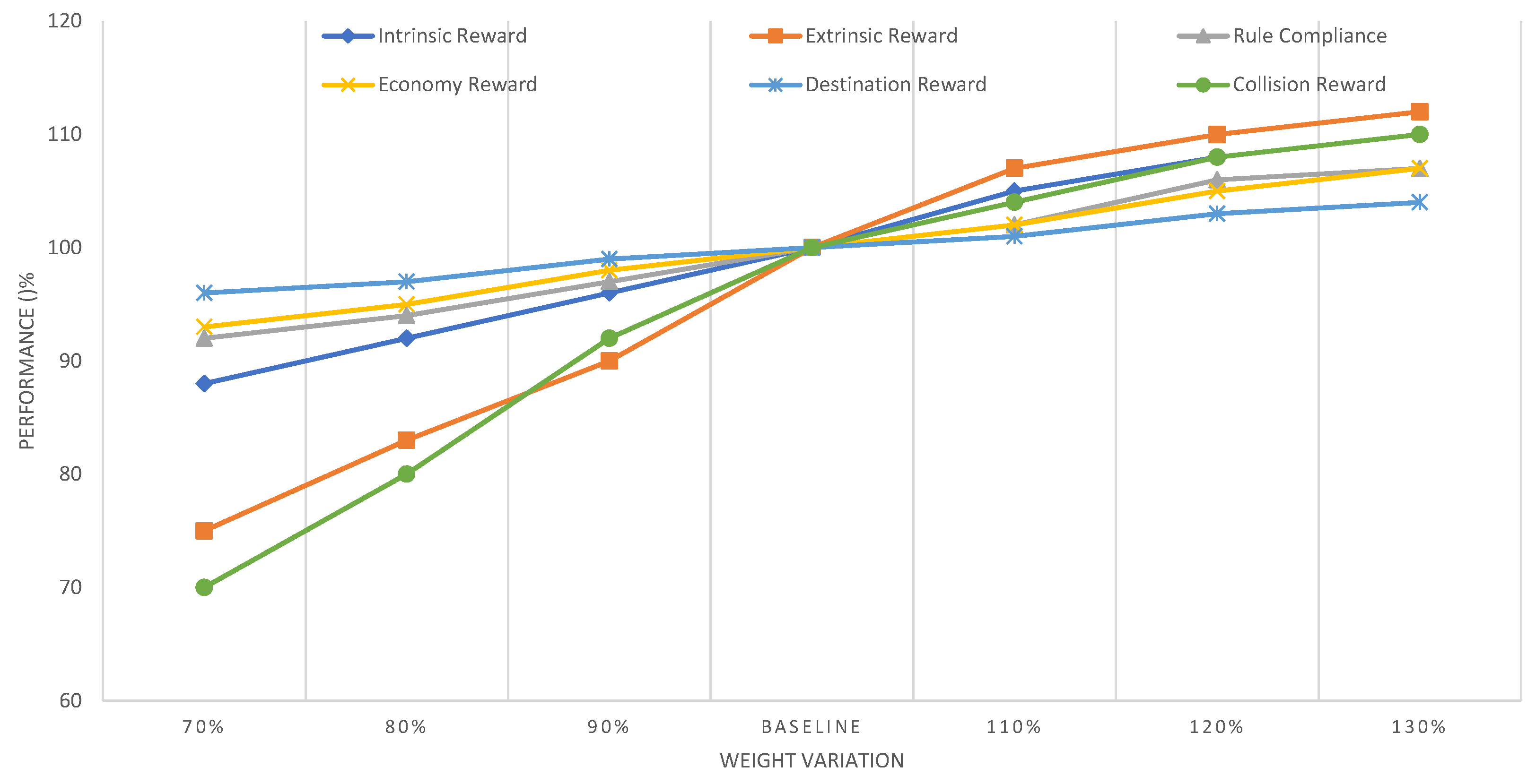
5.3. Reward Weighting Analysis

To verify the sensitivity of the proposed model to specific weight configurations, we analyze the performance variance across various weight values for each component. Figure 10 illustrates the sensitivity of key performance metrics to variations in component weights.
The analysis reveals that the model is most sensitive to the safety reward weight ( w s ), with a 20% reduction in this weight, potentially leading to unsafe navigation decisions. Conversely, the model demonstrates relatively low sensitivity to destination reward weight ( w d ), suggesting that this component provides useful guidance but is not critical for safe navigation. The intrinsic reward weight ( w i ) shows an interesting pattern: performance improves as w i increases from 0.7 to 1.0 and then slightly degrades for w i 1.0 . This suggests that balancing intrinsic and extrinsic rewards is crucial for the navigation objective.
Based on this comprehensive analysis, we could conclude that the integration of intrinsic rewards with properly weighted extrinsic components provides the optimal reward for collision avoidance. This balanced reward design promotes effective navigation across various scenarios: w i = 1.0 ,   w e = 1.0 ,   w d = 1.0 ,   w s = 1.0 ,   w m = 0.9 ,   w c = 1.1 , and w e 1 = 1.1 . This exploration through rewards with the practical concerns of safety, efficiency, and rule compliance leads to faster convergence and more robust performance.

6. Analysis of Experimental Results

6.1. Comparative Performance Analysis

To evaluate our proposed approach, we conduct systematic comparisons against three reference points: real AIS data, reinforcement learning algorithms, and the traditional collision avoidance method, as well as different environmental conditions. This multi-faceted comparison provides a holistic assessment of the model’s practical applicability and relative advantages. Table 5 presents the performance comparison.
The proposed model achieves higher success rates of 97.6% compared to other methods. While the computational efficiency of VO method is better, other methods illustrate lower success rates with PPO at 93.2% and DDPG at 89.5%. For reinforcement learning methods, all approaches perform reasonably well in standard encounters, but the proposed formulation has a clear advantage in success rate. The A3C algorithm achieves faster computation time but could not match the proposed model’s navigation performance. When compared to AIS trajectory data, our model demonstrates wider passing distances (0.648 nmi vs. 0.515 nmi).

6.2. The Influence of Ship Density

Ship density significantly influences decision-making efficiency in maritime navigation. As the number of ships increases, the complexity of navigational decisions escalates, resulting in substantial impacts on safety, efficiency, and operational effectiveness. To evaluate the proposed model’s performance and stability, we conduct experiments with 2, 4, 6, 8, and 10 ships in the same navigational area (a 10 × 10 nmi section of an inland waterway). Table 6 presents the key performance metrics across different ship densities. The results demonstrate that while computational requirements increase with ship density, the algorithm maintains acceptable performance. Response times remain under 550 ms even in high-density scenarios, suitable for real-time decision-making given typical vessel response times.

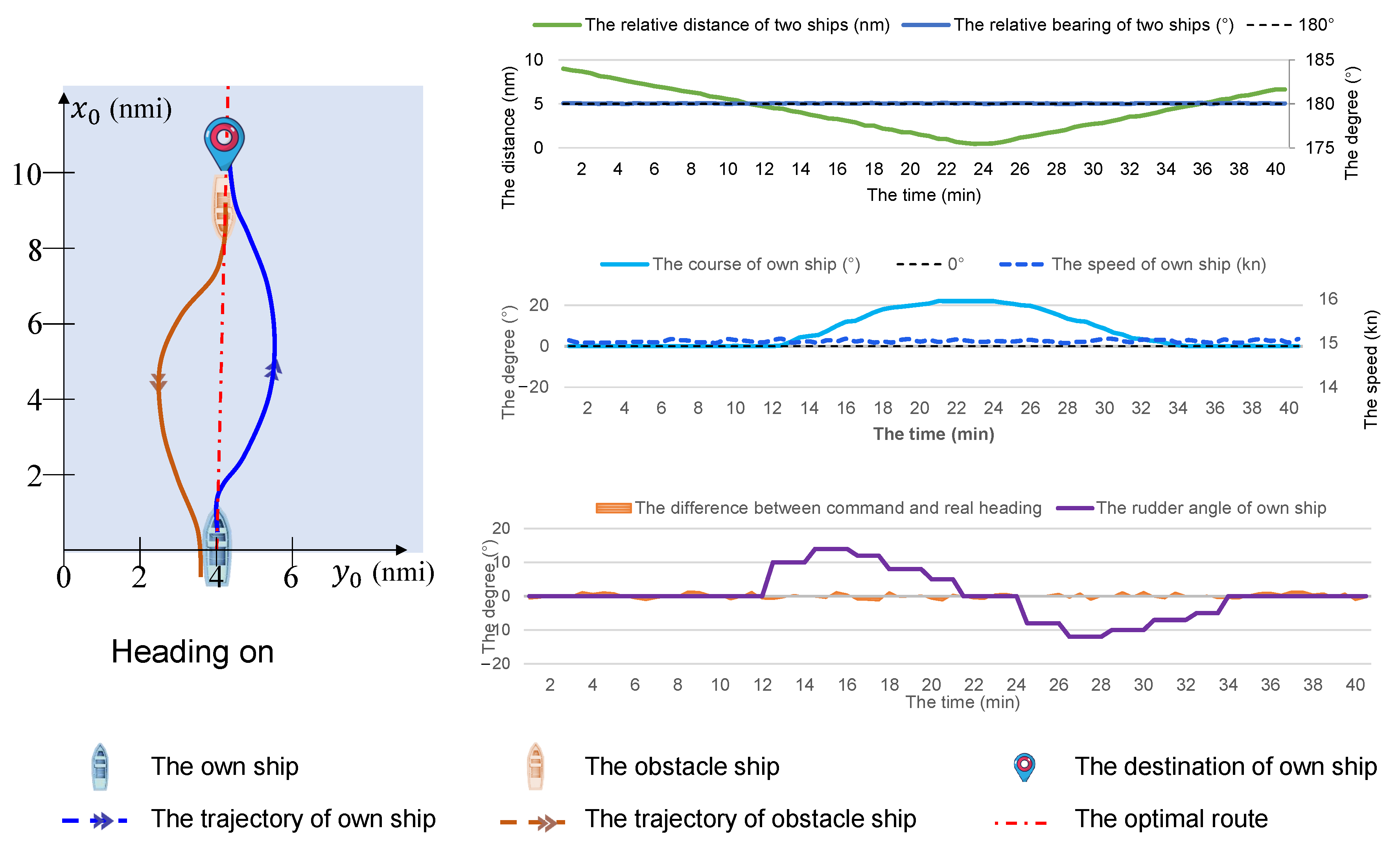
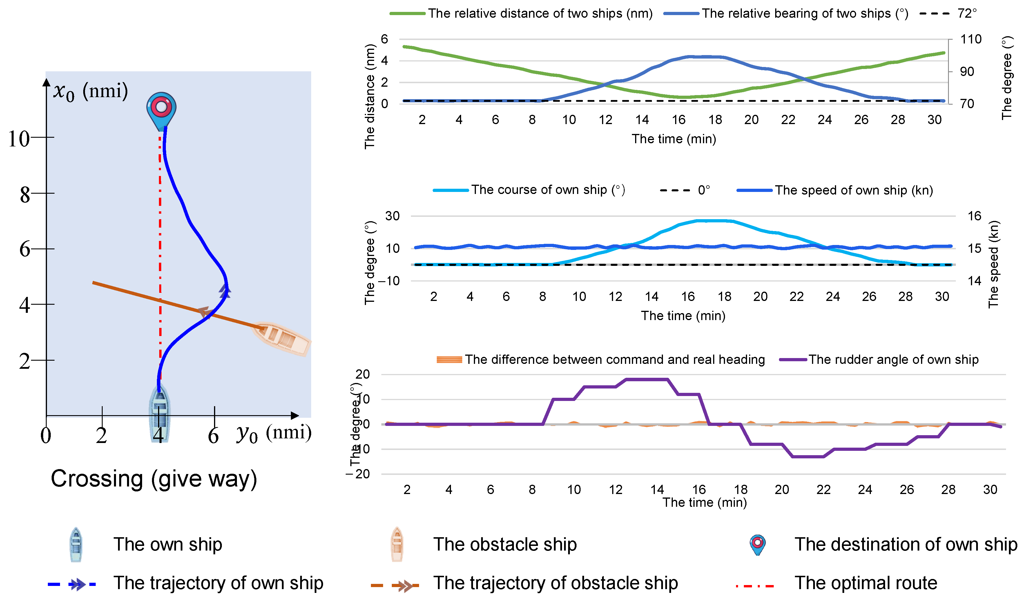
6.3. Typical Two-Ship Encounter Situation

Three typical situations, including head-on, overtaking, and crossing, are simulated to assess compliance with collision avoidance rules and the security of the decision-making method. The three typical two-vessel encounter scenarios are simulated in a relatively broad inland waterway, such as the middle and lower reaches of the Yangtze River water area. The initial parameters for the three typical encounters are provided in Table 7.
(a) Head-on encounter: For the head-on situation, the relative distance between the two ships initially decreases and then increases, as shown in Figure 11. The closest point of approach occurs at approximately 24 min with a minimum distance greater than the collision risk threshold, successfully avoiding collision with the obstacle ship. The relative bearing remains relatively stable around 180 degrees, indicating a typical head-on encounter situation. The course and speed changes of the own ship are shown in the middle graph. The own ship maintains its initial course of 0 degrees for about 11 min. Upon detecting the head-on approaching vessel, the own ship alters its course to starboard, reaching a maximum of 22.5 degrees over the next 12 min. Subsequently, to return to its optimal route, the course gradually decreases, briefly going to around 0 degrees at around 35 min before stabilizing. The speed of the own ship remains relatively constant at approximately 15 knots throughout the encounter, with only minor variations of about 0.5 knots because of the influence of water flow or wind. This stable speed profile suggests that the collision avoidance maneuver was primarily executed through course changes rather than speed adjustments. The bottom graph shows the rudder angle and the difference between commanded and actual heading. When executing the course change, the maximum rudder angle reaches about 14 degrees during the starboard turn, and later reaches about −12 degrees when returning. The difference between commanded and actual heading remains small (within 1–1.5 degrees), indicating precise rudder control and effective course-keeping throughout the maneuver.
(b) Crossing encounter (starboard crossing): In crossing encounters, this study focuses on the starboard crossing scenario where the own ship is the give-way vessel, as shown in Figure 12. The port crossing scenario follows analogous principles of collision avoidance with the obstacle ship as the give-way vessel.
The trends in relative distance and bearing show a characteristic pattern. The distance between the two ships gradually decreases to a minimum value of around 0.65 nmi at approximately 16 min, which exceeds the calculated collision diameter, ensuring safe passage. The relative bearing changes from about 72 degrees to approximately 99 degrees during the encounter and then returns to around 72 degrees after the own ship passes the obstacle ship. The obstacle ship maintains its course and speed throughout this process. The own ship maintains a course of 0 degrees for the first 9 min. The course increases to approximately 27 degrees at around 17 min, and then gradually decreases to return to the original track. The speed remains relatively stable at around 15 knots throughout most of the maneuver, with only minor variations during the course changes. During the initial course change, the maximum rudder angle reaches about 14 degrees to starboard. When returning to the original course, the rudder angle reaches about −12 degrees. Throughout the entire maneuver, the rudder movements are deliberate and controlled. The difference between commanded and actual heading remains small.
(c) Overtaking encounter: The overtaking encounter, as illustrated in Figure 13, spans approximately 25 min from initiation to completion.
During this encounter, the relative distance between vessels reaches its minimum of approximately 0.95 nmi at 12 min. The relative bearing data show a gradual increase to approximately 17 degrees before returning to near 0 degrees, indicating a successful port-side overtaking. The own ship’s maneuvering characteristics demonstrate a controlled overtaking sequence. The course alteration begins at approximately 3 min, reaching a maximum deviation before gradually returning to the original track. Speed management remains stable throughout the maneuver, maintaining approximately 15 knots with only minor variations. Initially maintaining around 15 degrees during the approach phase, the rudder angle transitions to negative values (approximately −9 degrees) during the return-to-track phase. The difference between commanded and actual heading remains consistently small (within 1–2 degrees), indicating precise heading control despite the extended duration of the overtaking maneuver. In conclusion, it was observed that the own ship effectively demonstrated collision avoidance capabilities across all three types of ship encounters.

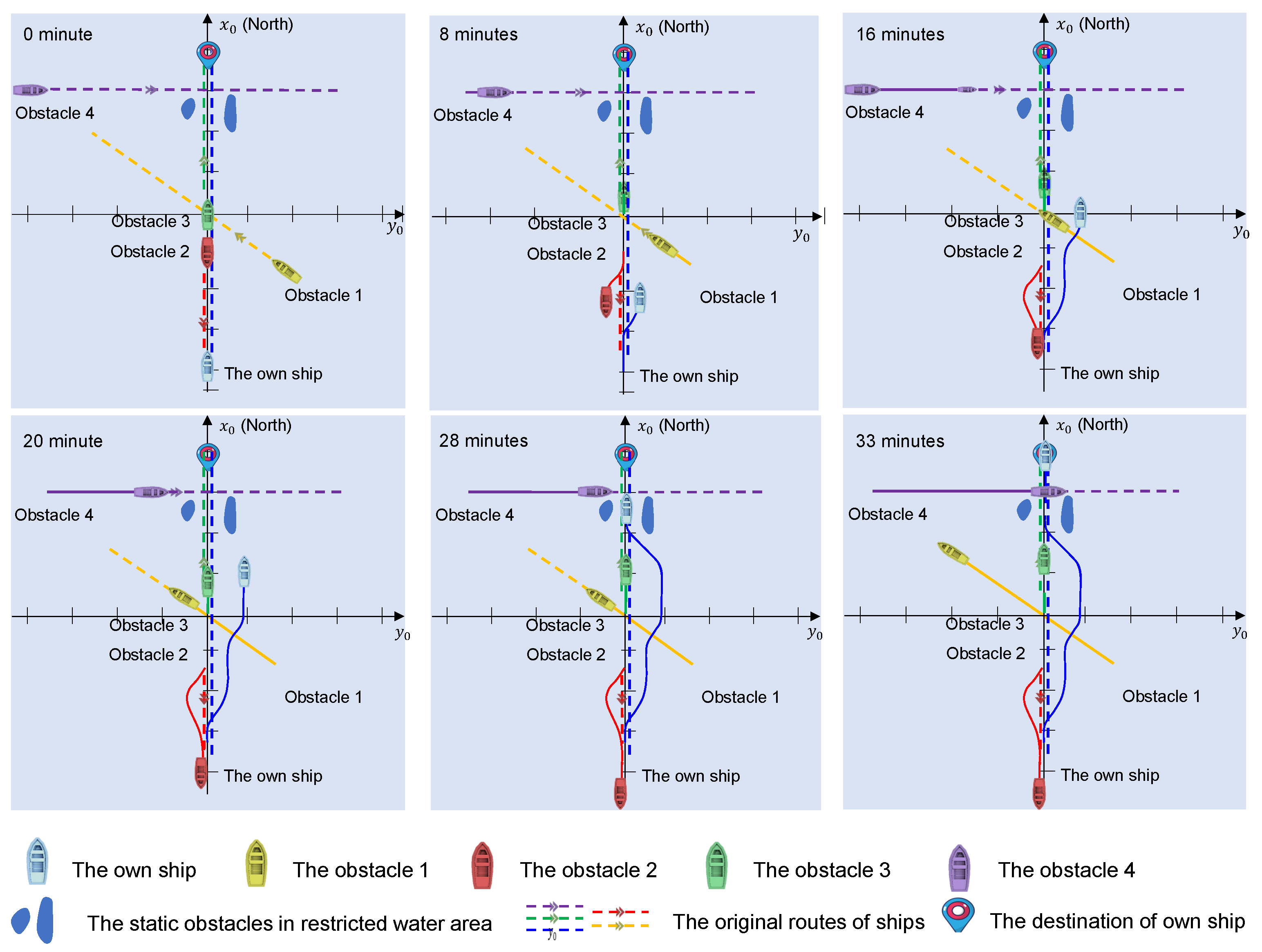
6.4. Multi-Ship Encounter Scenario

In inland waterways, there are often areas that are impassable. To evaluate the decision-making prowess of the algorithm proposed, we designed a simulation experiment incorporating both dynamic and static obstacles. The multi-ship encounter scenario considers a narrow channel confined by the static obstacles (e.g., navigational markers or natural obstacles), such as the navigation channels in the mountainous upper reaches of the Yangtze River. The initial parameters for the own ship and obstacles are presented in Table 8. The initial parameters for multiple ships involve five vessels, all with identical dimensions of 66 m in length and 11 m in width. The own ship begins at position (−4, 0) nmi with a course of 0° and speed of 15 knots, heading toward the target position (4, 0) nmi. Ship 1 starts at (−2, 2) nmi with a course of 315° and speed of 10.6 knots, moving toward (2, −2) nmi. Ship 2 initiates from (−1, 0) nmi with a course of 180° and speed of 9 knots, heading to (−5, 0) nmi. Ship 3 starts at (0, 0) nmi with a course of 0° and a slower speed of 3 knots, moving toward (4, 0) nmi. Ship 4 begins at position (3, −4) nmi with a course of 90° and speed of 8.6 knots, targeting position (3, 3) nmi.
The trajectories and related parameters of ship collision avoidance are shown in Figure 14 and Figure 15, respectively. The own ship maintains a course of 0 degrees at a steady speed of approximately 15 knots. When encountering obstacle 2 in a head-on situation, the two ships both turn to their own starboard sides. The own ship gradually increases its course to approximately 19 degrees. At 9 min, the own ship passes by the obstacle 2 at the shortest distance of 0.5 nmi. After that, the own ship maintains its course for about 6 min until it meets the obstacle 1. In order not to affect the navigation of obstacle 1, the own ship adjusts its course to starboard for another 6 degrees and passes by the obstacle 1 with the closest distance of 0.68 nmi. The own ship continues its current course for about 6 min and overtakes the obstacle 3 at 22 min. During this period, the obstacle 1 and obstacle 3 maintain their course and speed. After that, the own ship begins to return to the original route, and the obstacle 4 is crossing ahead of it at this time. There are static obstacles on both sides of the course, which means the channel is too narrow for the own ship to turn its direction. According to the rules, obstacle 4 has to wait for the own ship to pass. Therefore, the speed of obstacle 4 reduces to 0, and the own ship also reduces its speed from 15 kts to 13 kts to pass through the channel.
The course of the own ship changes along with the rudder angle. It is evident that the rudder angle changes in a stepped manner, which is commonly used in navigation. The ship will decelerate in advance when passing through narrow channels. Throughout the whole process, the difference between the commanded and real heading is lower than 2 degrees, which means the delay in the ship’s response is small.

6.5. Limitations and Implementation Challenges

The proposed model faces several key limitations. First, the state space representation assumes discrete and fully observable states, which may not effectively capture the continuous or observable nature of maritime environments. Second, the model assumes relatively stable environmental conditions and shows a limited ability to adapt to rapidly changing weather. Finally, the model’s performance heavily depends on training data representation, where rare events and edge cases may be underrepresented.
In addition, for long-term applicability to real-world navigation scenarios, the proposed model should be compatible with existing navigation systems. These limitations suggest that while the model shows promise, careful consideration is needed for real-world deployment.

7. Conclusions

To achieve multi-ship collision avoidance, this study proposes a reward-driven reinforcement learning collision avoidance model, which could comprehensively consider the collision risk, economy reward, and penalty for collision avoidance rules, and provide effective and safe collision avoidance actions. In the experiments, the own ship could pass by obstacle ships within a safe distance in various encounter situations, including multiple static and dynamic situations. Several key conclusions can be drawn from the experimental results. (1) The proposed algorithm could provide effective decisions for safe navigation in inland waterways. (2) The design of the reward function, which needs to balance the economy and safety of ships, could have significant effects on the collision avoidance strategy.
In future research, the following directions should be explored: (1) Developing more sophisticated state space representations to better handle continuous maritime environments. (2) For long-term applicability to real-world navigation scenarios, the proposed model should be compatible with existing navigation systems.

Author Contributions

Methodology, Y.W.; software, S.G.; formal analysis, Z.Z.; data curation, D.W.; writing—original draft, S.G., Z.Z., Y.W. and D.W.; writing—review and editing, S.G., Z.Z. and Y.W. All authors have read and agreed to the published version of the manuscript.

Funding

This research was funded by National Natural Science Foundation of China (NSFC) grant number 62003011.

Data Availability Statement

Restrictions apply to the availability of these data. Data was obtained from Yangtze River Waterway Bureau and are available with the permission of Yangtze River Waterway Bureau.

Conflicts of Interest

The authors declare no conflicts of interest.

References

  1. Aritua, B.; Cheng, L.; van Liere, R.; de Leijer, H. Blue Routes for a New Era: Developing Inland Waterways Transportation in China; World Bank Publications; World Bank Group: Washington, DC, USA, 2021. [Google Scholar]
  2. Chaal, M.; Ren, X.; BahooToroody, A.; Basnet, S.; Bolbot, V.; Banda, O.A.V.; Van Gelder, P. Research on risk, safety, and reliability of autonomous ships: A bibliometric review. Saf. Sci. 2023, 167, 106256. [Google Scholar] [CrossRef]
  3. Namgung, H.; Kim, J.S. Collision risk inference system for maritime autonomous surface ships using COLREGs rules compliant collision avoidance. IEEE Access 2021, 9, 7823–7835. [Google Scholar] [CrossRef]
  4. Huang, Y.; Chen, L.; Chen, P.; Negenborn, R.R.; Van Gelder, P. Ship collision avoidance methods: State-of-the-art. Saf. Sci. 2020, 121, 451–473. [Google Scholar] [CrossRef]
  5. Vagale, A.; Oucheikh, R.; Bye, R.T.; Osen, O.L.; Fossen, T.I. Path planning and collision avoidance for autonomous surface vehicles I: A review. J. Mar. Sci. Technol. 2021, 26, 1292–1306. [Google Scholar] [CrossRef]
  6. Singh, Y.; Sharma, S.; Sutton, R.; Hatton, D.; Khan, A. A constrained A* approach towards optimal path planning for an unmanned surface vehicle in a maritime environment containing dynamic obstacles and ocean currents. Ocean Eng. 2018, 169, 187–201. [Google Scholar] [CrossRef]
  7. Xue, Y.; Clelland, D.; Lee, B.; Han, D. Automatic simulation of ship navigation. Ocean Eng. 2011, 38, 2290–2305. [Google Scholar] [CrossRef]
  8. Liu, C.; Mao, Q.; Chu, X.; Xie, S. An improved A-star algorithm considering water current, traffic separation and berthing for vessel path planning. Appl. Sci. 2019, 9, 1057. [Google Scholar] [CrossRef]
  9. Wang, H.; Zhou, J.; Zheng, G.; Liang, Y. HAS: Hierarchical A-Star algorithm for big map navigation in special areas. In Proceedings of the 2014 5th International Conference on Digital Home, Guangzhou, China, 28–30 November 2014; IEEE: New York, NY, USA, 2014; pp. 222–225. [Google Scholar]
  10. Kouzuki, A.; Hasegawa, K. Automatic collision avoidance system for ships using fuzzy control. J. Kansai Soc. Nav. Arch. Jpn. 1987, 205, 1–10. [Google Scholar]
  11. Denker, C.; Baldauf, M.; Fischer, S.; Hahn, A.; Ziebold, R.; Gehrmann, E.; Semann, M. E-Navigation based cooperative collision avoidance at sea: The MTCAS approach. In Proceedings of the 2016 European Navigation Conference (ENC), Helsinki, Finland, 30 May–2 June 2016; IEEE: New York, NY, USA, 2016; pp. 1–8. [Google Scholar]
  12. Zhao, Y.; Li, W.; Shi, P. A real-time collision avoidance learning system for Unmanned Surface Vessels. Neurocomputing 2016, 182, 255–266. [Google Scholar] [CrossRef]
  13. Chen, P.; Huang, Y.; Mou, J.; Van Gelder, P. Probabilistic risk analysis for ship-ship collision: State-of-the-art. Saf. Sci. 2019, 117, 108–122. [Google Scholar] [CrossRef]
  14. Degre, T.; Lefevre, X. A collision avoidance system. J. Navig. 1981, 34, 294–302. [Google Scholar] [CrossRef]
  15. Bareiss, D.; Van den Berg, J. Generalized reciprocal collision avoidance. Int. J. Robot. Res. 2015, 34, 1501–1514. [Google Scholar] [CrossRef]
  16. Huang, Y.; Chen, L.; Van Gelder, P. Generalized velocity obstacle algorithm for preventing ship collisions at sea. Ocean Eng. 2019, 173, 142–156. [Google Scholar] [CrossRef]
  17. Wilson, P.; Harris, C.; Hong, X. A line of sight counteraction navigation algorithm for ship encounter collision avoidance. J. Navig. 2003, 56, 111–121. [Google Scholar] [CrossRef]
  18. Alonso-Mora, J.; Gohl, P.; Watson, S.; Siegwart, R.; Beardsley, P. Shared control of autonomous vehicles based on velocity space optimization. In Proceedings of the 2014 IEEE International Conference on Robotics and Automation (ICRA), Hong Kong, China, 31 May–7 June 2014; IEEE: New York, NY, USA, 2014; pp. 1639–1645. [Google Scholar]
  19. Fujii, Y.; Shiobara, R. The analysis of traffic accidents. J. Navig. 1971, 24, 534–543. [Google Scholar] [CrossRef]
  20. Goodwin, E.M. A statistical study of ship domains. J. Navig. 1975, 28, 328–344. [Google Scholar] [CrossRef]
  21. Szlapczynski, R.; Szlapczynska, J. Review of ship safety domains: Models and applications. Ocean Eng. 2017, 145, 277–289. [Google Scholar] [CrossRef]
  22. Shinar, J.; Steinberg, D. Analysis of optimal evasive maneuvers based on a linearized two-dimensional kinematic model. J. Aircr. 1977, 14, 795–802. [Google Scholar] [CrossRef]
  23. Coldwell, T. Marine traffic behaviour in restricted waters. J. Navig. 1983, 36, 430–444. [Google Scholar] [CrossRef]
  24. Xu, P.; Lan, D.; Yang, H.; Zhang, S.; Kim, H.; Shin, I. Ship formation and route optimization design based on improved PSO and DP algorithm. IEEE Access 2025, 13, 15529–15546. [Google Scholar] [CrossRef]
  25. Chen, J.; Zhou, L.; Ding, S.; Li, F. Numerical simulation of moored ships in level ice considering dynamic behavior of mooring cable. Mar. Struct. 2025, 99, 103716. [Google Scholar] [CrossRef]
  26. Statheros, T.; Howells, G.; Maier, K.M. Autonomous ship collision avoidance navigation concepts, technologies and techniques. J. Navig. 2008, 61, 129–142. [Google Scholar] [CrossRef]
  27. Tsou, M.C.; Hsueh, C.K. The study of ship collision avoidance route planning by ant colony algorithm. J. Mar. Sci. Technol. 2010, 18, 16. [Google Scholar] [CrossRef]
  28. Cho, Y.; Han, J.; Kim, J. Efficient COLREG-compliant collision avoidance in multi-ship encounter situations. IEEE Trans. Intell. Transp. Syst. 2020, 23, 1899–1911. [Google Scholar] [CrossRef]
  29. He, Z.; Liu, C.; Chu, X.; Negenborn, R.R.; Wu, Q. Dynamic anti-collision A-star algorithm for multi-ship encounter situations. Appl. Ocean Res. 2022, 118, 102995. [Google Scholar] [CrossRef]
  30. Karbowska-Chilinska, J.; Koszelew, J.; Ostrowski, K.; Kuczynski, P.; Kulbiej, E.; Wolejsza, P. Beam search Algorithm for ship anti-collision trajectory planning. Sensors 2019, 19, 5338. [Google Scholar] [CrossRef] [PubMed]
  31. Xu, Q. Collision avoidance strategy optimization based on danger immune algorithm. Comput. Ind. Eng. 2014, 76, 268–279. [Google Scholar] [CrossRef]
  32. Sawada, R.; Sato, K.; Majima, T. Automatic ship collision avoidance using deep reinforcement learning with LSTM in continuous action spaces. J. Mar. Sci. Technol. 2021, 26, 509–524. [Google Scholar] [CrossRef]
  33. Chun, D.H.; Roh, M.I.; Lee, H.W.; Ha, J.; Yu, D. Deep reinforcement learning-based collision avoidance for an autonomous ship. Ocean Eng. 2021, 234, 109216. [Google Scholar] [CrossRef]
  34. Wang, Y.; Xu, H.; Feng, H.; He, J.; Yang, H.; Li, F.; Yang, Z. Deep reinforcement learning based collision avoidance system for autonomous ships. Ocean Eng. 2024, 292, 116527. [Google Scholar] [CrossRef]
  35. Xie, S.; Chu, X.; Zheng, M.; Liu, C. A composite learning method for multi-ship collision avoidance based on reinforcement learning and inverse control. Neurocomputing 2020, 411, 375–392. [Google Scholar] [CrossRef]
  36. Rongcai, Z.; Hongwei, X.; Kexin, Y. Autonomous collision avoidance system in a multi-ship environment based on proximal policy optimization method. Ocean Eng. 2023, 272, 113779. [Google Scholar] [CrossRef]
  37. Zheng, K.; Zhang, X.; Wang, C.; Zhang, M.; Cui, H. A partially observable multi-ship collision avoidance decision-making model based on deep reinforcement learning. Ocean Coast. Manag. 2023, 242, 106689. [Google Scholar] [CrossRef]
  38. Yang, X.; Han, Q. Improved reinforcement learning for collision-free local path planning of dynamic obstacle. Ocean Eng. 2023, 283, 115040. [Google Scholar] [CrossRef]
  39. Yang, L.; Li, L.; Liu, Q.; Ma, Y.; Liao, J. Influence of physiological, psychological and environmental factors on passenger ship seafarer fatigue in real navigation environment. Saf. Sci. 2023, 168, 106293. [Google Scholar] [CrossRef]
  40. Sui, Z.; Wen, Y.; Huang, Y.; Song, R.; Piera, M.A. Maritime accidents in the Yangtze River: A time series analysis for 2011–2020. Accid. Anal. Prev. 2023, 180, 106901. [Google Scholar] [CrossRef]
  41. Tam, C.; Bucknall, R. Collision risk assessment for ships. J. Mar. Sci. Technol. 2010, 15, 257–270. [Google Scholar] [CrossRef]
  42. Davis, P.; Dove, M.; Stockel, C. A computer simulation of marine traffic using domains and arenas. J. Navig. 1980, 33, 215–222. [Google Scholar] [CrossRef]
  43. Pedersen, P.T. Collision and grounding mechanics. Proc. WEMT 1995, 95, 125–157. [Google Scholar]
  44. Friis-Hansen, P.; Ravn, E.; Engberg, P. Basic modelling principles for prediction of collision and grounding frequencies. In IWRAP Mark II Working Document; Technical University of Denmark: Kongens Lyngby, Denmark, 2008; pp. 1–59. [Google Scholar]
  45. Altan, Y.C. Collision diameter for maritime accidents considering the drifting of vessels. Ocean Eng. 2019, 187, 106158. [Google Scholar] [CrossRef]
  46. Pedersen, P.T.; Zhang, S. Collision analysis for MS Dextra. In Proceedings of the SAFER EURORO Spring Meeting, Nantes, France, 28 April 1999; Citeseer: Princeton, NJ, USA, 1999; Volume 28, pp. 1–33. [Google Scholar]
  47. Yoshimura, Y. Mathematical model for the manoeuvring ship motion in shallow water (2nd Report)-mathematical model at slow forward speed. J. Kansai Soc. Nav. Archit. 1988, 210, 77–84. [Google Scholar]
  48. Ogawa, A.; Koyama, T.; Kijima, K. MMG report-I, on the mathematical model of ship manoeuvring. Bull. Soc. Nav. Arch. Jpn. 1977, 575, 22–28. [Google Scholar]
  49. Miele, A.; Wang, T.; Chao, C.; Dabney, J. Optimal control of a ship for collision avoidance maneuvers. J. Optim. Theory Appl. 1999, 103, 495–519. [Google Scholar] [CrossRef]
  50. Debnath, A.K.; Chin, H.C. Navigational traffic conflict technique: A proactive approach to quantitative measurement of collision risks in port waters. J. Navig. 2010, 63, 137–152. [Google Scholar] [CrossRef]
  51. Zhang, L.; Meng, Q. Probabilistic ship domain with applications to ship collision risk assessment. Ocean Eng. 2019, 186, 106130. [Google Scholar] [CrossRef]
  52. Qu, X.; Meng, Q.; Suyi, L. Ship collision risk assessment for the Singapore Strait. Accid. Anal. Prev. 2011, 43, 2030–2036. [Google Scholar] [CrossRef]
  53. Yoshimura, Y. Mathematical model for manoeuvring ship motion (MMG Model). In Proceedings of the Workshop on Mathematical Models for Operations involving Ship-Ship Interaction, Tokyo, Japan, 4 August 2005; pp. 1–6. [Google Scholar]
Figure 1. The bumper model.
Symmetry 17 00613 g001
Figure 2. Coldwell’s domain.
Symmetry 17 00613 g002
Figure 3. The encounter situations (red, green, yellow, gray, and dark gray are starboard crossing (give way), port crossing (stand on), head-on, overtaking, and safe, respectively.).
Symmetry 17 00613 g003
Figure 5. The ship motion coordinate system.
Symmetry 17 00613 g005
Figure 6. The relative position between the own ship and the obstacle ship.
Symmetry 17 00613 g006
Figure 7. The line-of-sight (LOS) guidance.
Symmetry 17 00613 g007
Figure 8. The actor–critic algorithm-based collision avoidance strategy.
Symmetry 17 00613 g008
Figure 9. The training process of actor and critic networks.
Symmetry 17 00613 g009
Figure 10. Reward weighting analysis.
Symmetry 17 00613 g010
Figure 11. The head-on encounter situation.
Symmetry 17 00613 g011
Figure 12. The crossing encounter situation.
Symmetry 17 00613 g012
Figure 13. The overhead encounter situation.
Symmetry 17 00613 g013
Figure 14. The multi-ship encounter situation.
Symmetry 17 00613 g014
Figure 15. The parameters in the multi-ship encounter situation.
Symmetry 17 00613 g015
Table 1. The pseudocode of the training process.
Training: Update the Parameters of Actor and Critic Networks
1. Observe the state s t ;
2. Randomly sample action a t according to π ( | ˙ s t ; θ t ) ;
3. Perform a t and observe the new state s t + 1 and reward r t ;
4. Update parameters ω in the critic network using the TD error;
5. Update parameters θ in the actor network using the policy gradient method.
Table 2. Hyperparameters for the training of the actor–critic networks.
ParameterValue
Discount rate0.9
Max episodes8000
Max steps500
Batch size64
Sampling time30 s
Learning rate of actor network2 × 10−3
Learning rate of critic network1 × 10−3
Table 3. The scenario-specific convergence characteristics.
ScenariosEpisodes to ConvergeActor Final LossCritic Final LossTime to Converge (h)
A3CPPODDPGProposed
Model
A3CPPODDPGProposed
Model
A3CPPODDPGProposed
Model
A3CPPODDPGProposed
Model
Head-on45006000700050000.210.180.20.150.180.160.190.1312.516.719.413.9
Crossing46006100700049000.20.190.210.160.190.170.20.1412.816.919.413.6
Overtaking45006000680050000.230.180.20.150.180.150.190.1512.516.718.913.9
Multi-ship50006300750052000.230.20.220.160.220.190.210.1713.917.520.814.4
Table 4. Coefficient parameters of the ship motion model.
ParameterValueParameterValueParameterValueParameterValue
X u u ( 0 ) −0.0196 Y b 0.3979 N b 0.0992 1 t R 0.709
X b b −0.0082 Y r 0.0918 N r −0.0579 a H 0.28
X b r −0.1446 Y b b b 1.6016 N b b b 0.1439 x H / L −0.377
X r r 0.0125 Y b b r −0.2953 N b b r −0.3574 1 t 0.73
X b b b b 0.3190 Y b r r 0.4140 N b r r 0.0183 D p 2.5 m
J Z Z −0.0055 Y r r r −0.0496 N r r r −0.0207 ρ 1025 kg/m3
Table 5. Comparative performance analysis.
MethodSuccess Rate
(%)
Avg. Min. Distance
(nmi)
Computational Time
(ms)
Proposed model97.60.648410
PPO93.20.572438
A3C91.80.591392
DDPG89.50.484425
Velocity obstacle91.30.517335
AIS trajectory-0.515-
Table 6. Performance metrics across different ship densities.
Ship CountSuccess Rate
(%)
Avg. Comput. Time
(ms)
Min. Dist.
(nmi)
299.24100.698
497.84280.654
695.44550.633
893.14860.591
1090.55240.534
Table 7. The initial parameters for three encounters.
ShipsLength
(m)
Width
(m)
Initial
Course (°)
Initial
Speed (kts)
Initial
Position (nmi)
Target
Position (nmi)
Encounter
Situations
Own ship6611015(0, 4)(10, 4)-
Ship 1661118010(9, 4)(0, 3.8)Head-on
Ship 2661128015.5(3.5, 8)(6.2, 0)Crossing
Ship 3661107(1.5, 4)(10, 4)Overtaking
Table 8. The initial parameters for multiple ships.
ShipsLength
(m)
Width
(m)
Initial
Course
(°)
Initial
Speed
(kts)
Initial
Position
(nmi)
Target
Position
(nmi)
Own ship6611015(−4, 0)(4, 0)
Ship 1661131510.6(−2, 2)(2, −2)
Ship 266111809(−1, 0)(−5, 0)
Ship 3661103(0, 0)(4, 0)
Ship 46611908.6(3, −4)(3, 3)
Disclaimer/Publisher’s Note: The statements, opinions and data contained in all publications are solely those of the individual author(s) and contributor(s) and not of MDPI and/or the editor(s). MDPI and/or the editor(s) disclaim responsibility for any injury to people or property resulting from any ideas, methods, instructions or products referred to in the content.

