Lie Group Intrinsic Mean Feature Detectors for Real-Time Industrial Surface Defect Detection

Abstract

In the actual industrial production environment, the surface defects of products are subtle, and the number of different types of defect data samples is also quite small. Most deep learning models rely on a large number of training samples and parameters to achieve high-precision defect detection. At the same time, the edge computing layer in the actual industrial environment may also encounter transmission delays and insufficient resources. Training a proper model for a specific type of surface defect while simultaneously satisfying the real-time accuracy of defect detection is still a challenging task. To effectively deal with the above challenges, we propose an edge-cloud computing defect detection model based on the intrinsic mean feature detector in the Lie Group space. The modules in the model adopt a symmetrical structure, which can extract related features more effectively. Different from existing models, this model utilizes the Lie Group space intrinsic mean feature as a metric to characterize the essential attributes of different types of surface defects. In addition, we propose an intrinsic mean attention mechanism in the Lie Group manifold space that is easy to implement at the edge service layer without increasing the number of model parameters, thereby enhancing the detection performance of tiny surface defects. Extensive experiments on three publicly available and challenging datasets reveal the superiority of our model in terms of detection accuracy, real-time detection, number of parameters, and computational performance. In addition, our proposed model also shows competitiveness and advantages compared with state-of-the-art models.

1. Introduction

The rapid development of the Internet of Things (IoT) and artificial intelligence (AI) technology has accelerated the pace of the Industry 5.0 era, and the variety and quantity of intelligent IoT devices have shown exponential growth. According to incomplete statistics, the global number of IoT devices has increased from 8.74 billion in 2020 to 25.4 billion in 2030 [1,2]. The exponential growth in the number of IoT devices and the rapid development and application of 5G and 6G technologies have promoted their rapid application in multiple industries and fields such as intelligent manufacturing [3], industrial control systems [4], and Internet of vehicles (IoVs) [5]. However, the data collected by various IoT devices include images, text, and real-time high-capacity streaming media data, which brings great challenges to application scenarios that require real-time data processing.

Surface defect detection (SDD) has always been one of the important tasks in real-time detection in IoT intelligent manufacturing. The main reason for its occurrence is that during the manufacturing process, product defects (e.g., surface scratches, damage) occur due to factors such as technological level and working environment. Surface defects can affect the efficiency of enterprise production and reduce customer satisfaction. It is understood that some companies still utilize manual detection methods to detect surface defects in their products [6]. Manual detection has problems such as a heavy workload, long staff training cycles [7], low detection efficiency [8], and detection delays due to the increase in the number of products, which cannot satisfy the requirements of real-time detection in actual production processes.

In fact, real-time detection of surface defects is still quite a challenging task. Specifically, it is manifested in the following aspects:

• The data collected by IoT devices have the characteristics of high dimensionality and large capacity, which not only poses a challenge to intelligent devices with limited resources but also makes defects difficult to detect [9].
• The data are usually in a streaming format (such as visual data or environmental data), which increases the difficulty of data labeling. Therefore, real-time detection of surface defects should be efficient, scalable, and have a certain sensitivity to anomalies and defects [10].

In the actual industrial production process, the speed and quality of SSD are the two most important factors, which directly affect the company’s profits [11]. Typically, we utilize a cloud-based computing model to complete SSD. Although the cloud-based computing model has a large storage space and computing power, it still has many problems such as transmission delay [12], insufficient resources [13], and privacy security [14], and the real-time detection of surface defects is difficult to guarantee. To address such problems, scholars proposed a novel service paradigm, the multi-access edge-cloud computing (MEC) model, which enables resource-limited IoT devices to send captured data samples to edge servers for processing through a network (wired or wireless). In a real production environment, MEC can deploy deep learning models on edge servers to provide real-time SSD services for the surrounding IoT devices [3].

Although the MEC model can provide real-time detection services, it still has some shortcomings. The deep learning model deployed on the edge server requires a large number of training samples [15,16]. However, in the actual industrial production environment, the surface defects of the product are quite tiny, and the number of defect data samples is small, which directly affects the detection performance of the deep learning models [17,18]. Scholars have proposed transfer learning models, which can pre-train the model from the source domain dataset containing a large number of data samples, and then fine-tune the pre-trained model by the target domain dataset containing a small number of data samples. This model can solve the problem of insufficient training samples [19,20]. However, this model is based on the assumption that the source and target domain datasets have the same (or similar) data distribution. In the actual production process, the source and target domains may not necessarily satisfy the above assumptions. Therefore, it is a fundamental problem to study how to efficiently combine MEC and deep learning models to improve the speed and quality of SSD in actual industrial production.

To address the above problems, we explore the three-layer structure model of MEC. The modules in the model adopt a symmetrical structure, which can extract related features more effectively. Firstly, we make full use of the advantages of large storage capacity and strong computing power of cloud servers, store the data set on the cloud server, and pre-train the detection model (i.e., the universal detection model) through this data set. Then, the pre-trained universal detection model is sent and deployed to the edge server around the IoT device. Finally, the new data sample information captured by IoT devices is utilized to update the original universal detection model, so that the updated detection model can perform more accurate and efficient detection.

In summary, the main contributions of this study are as follows:

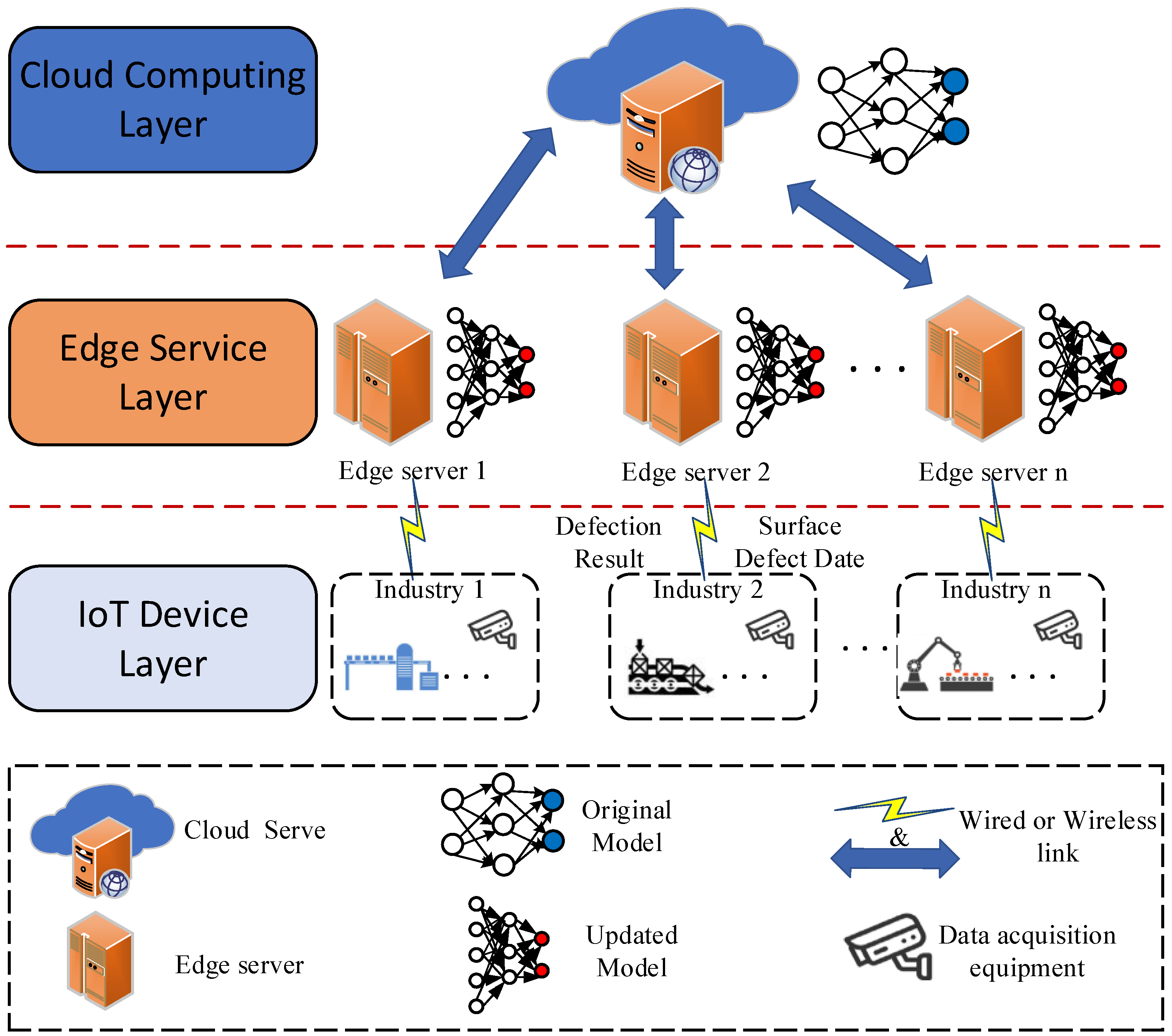
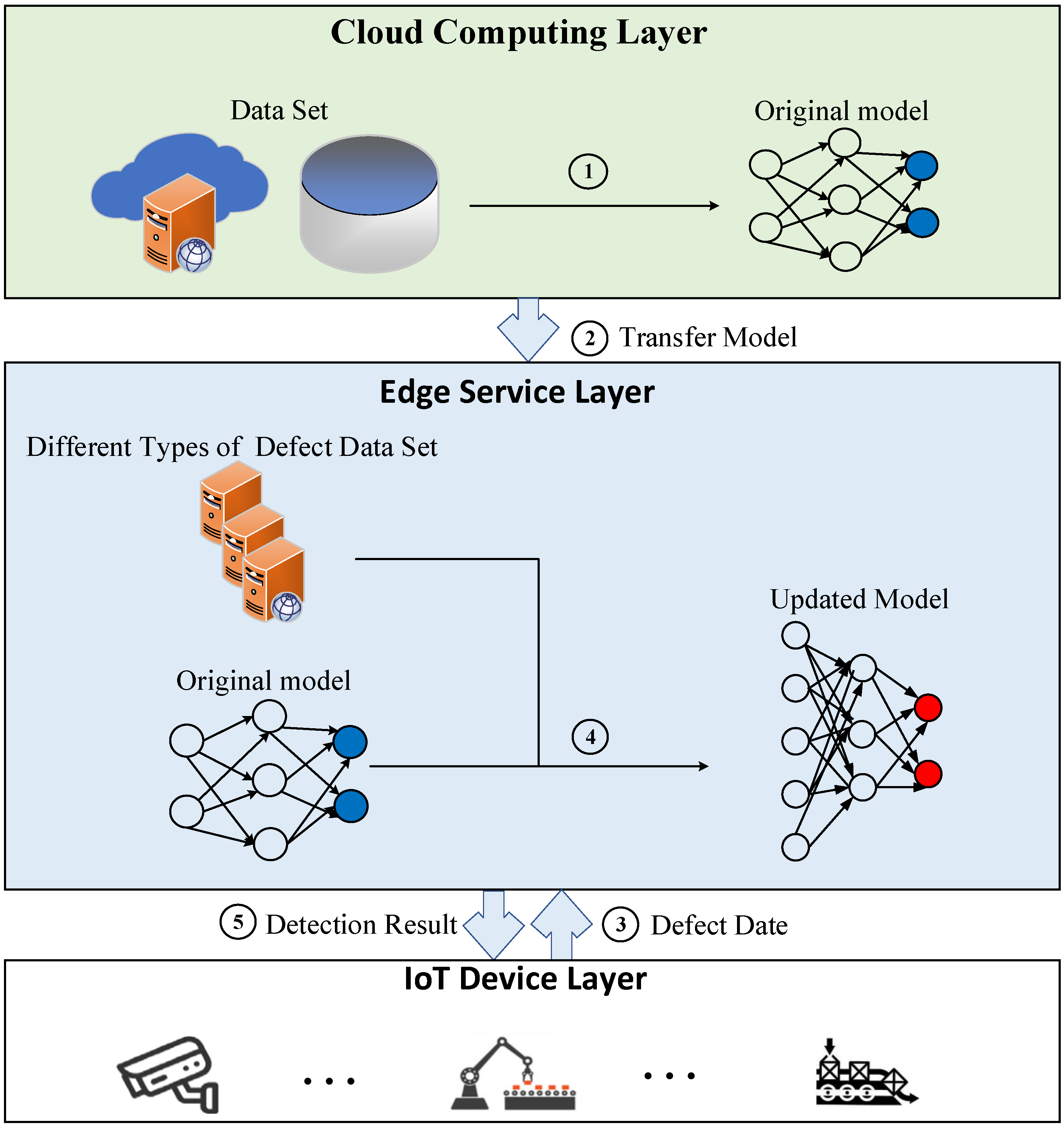
• To improve the speed and quality of SSD, we propose a three-layer structure model of MEC. In this model, the universal detection model trained on the cloud server is deployed to the edge server in advance and then updated according to the new data samples captured by IoT devices, so that the updated detection model shows better performance. The model can reduce the training time and improve the performance of tiny detection with limited data samples.
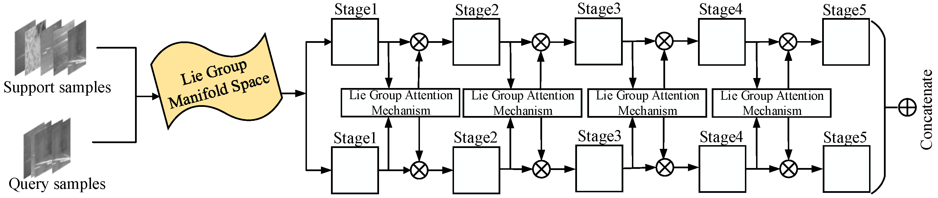
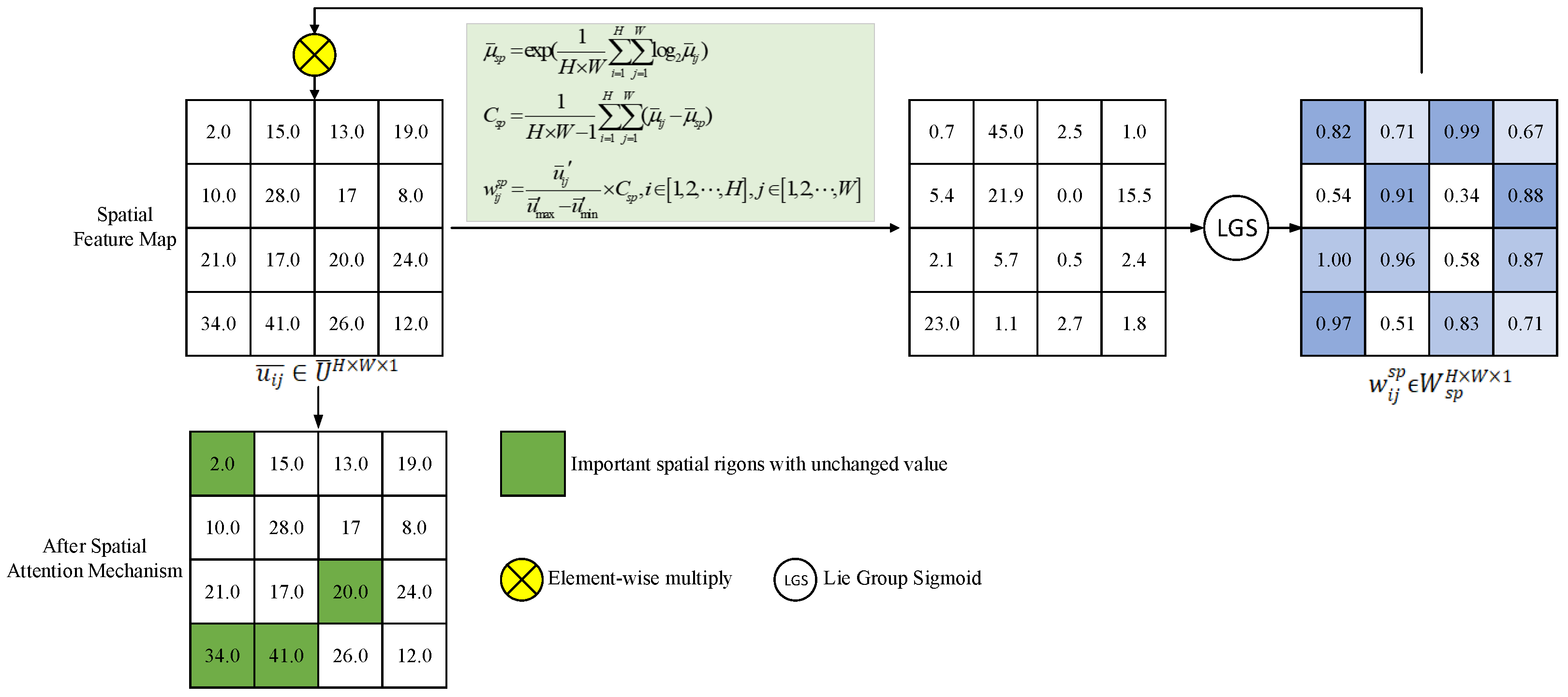
• To satisfy the real-time and efficiency of SSD, we propose an attention mechanism based on the intrinsic mean in the Lie Group manifold space. This mechanism utilizes the Lie Group manifold space calculation method instead of traditional operations such as pooling and convolution, which can efficiently locate the crucial features of tiny surfaces, effectively reduce the number of parameters of the model, avoid the selection and fine-tuning of hyperparameters, and better achieve the trade-off between detection accuracy and real-time performance.
• To verify the feasibility and performance of our proposed model through detailed experimental comparison. The experimental results show that our proposed model can effectively reduce the load on the edge server and satisfy the high-quality performance requirements of real-time detection; that is, our model is competitive with other state-of-the-art models in terms of improving the accuracy and speed of surface detection and reducing the detection delay.

2. Related Work

2.1. Defect Detection Based on Edge-Cloud Computing

In the Industry 5.0 scenario, a large number of resource-constrained IoT devices undertake computation-intensive tasks such as defect detection, resulting in detection delays and low production efficiency. To address such problems, scholars have proposed models based on edge or cloud computing. Zhang et al. [21] proposed a lightweight model that utilizes offline training and an online scaling mode for detection. Tang et al. [22] proposed Markov decision-based task offloading optimization to improve inference and detection speed. Zhu et al. [23] optimized the DenseNet model to improve resource-constrained IoT device detection ability. Xu et al. [24] proposed a cloud computing real-time detection model based on Lie Group manifold space, which contained a three-layer structure and realized efficient detection through the classification method of the Lie Group intrinsic mean. The above models mainly consider training the model at the cloud or edge and do not fully consider edge-cloud collaboration [3].

To fully consider the relationship between edge-cloud collaboration, scholars have proposed a series of computing models based on edge-cloud collaboration to achieve detection tasks. Liang et al. [25] proposed an edge-cloud collaborative detection model based on Edge YOLO, which makes full use of the advantages of cloud computing and reduces the load on IoT devices. Zhao et al. [26] proposed an edge-cloud collaborative detection model based on the industrial IoT architecture, which utilizes the advantages of the cloud layer to store data sets and utilizes transfer learning to fine-tune the detection model. Tang et al. [27] proposed a highly sensitive detection model with a two-stage algorithm. Wu et al. [28] proposed a blockchain-enabled IoT-edge-cloud computing model, which takes full advantage of MEC and mobile cloud computing.

2.2. Defect Detection Based on Deep Learning

Scholars have also proposed many defect detection models based on deep learning. In 2014, Girshick et al. [29] proposed the R-CNN model and first applied it in the field of detection. In 2015, Girshick [30] proposed a Fast-RCNN algorithm based on previous research and combined loss function and bounding box for selection. In the same year, Ren et al. [31] proposed the Faster-RCNN model based on Girshick’s research, which differs from the above models in that it used a neural network model instead of a selective algorithm. The main feature of the above model is to improve the accuracy of defect detection, but it also leads to another problem, which is the delay of defect detection. Nuanmeesri [32] proposed a hybrid attention mechanism for classifying avocados on resource-constrained devices. Nuanmeesri [33] proposed spectral-based hybrid deep learning for Hass avocado ripeness classification. Nuanmeesri et al. [34] proposed a transfer learning network model for classifying different types of aquaculture water quality.

To address the problem of defect detection delay, scholars have conducted in-depth research on detection accuracy and detection delay, and a series of models have been proposed. Aboelwafa et al. [35] proposed a model for detecting industrial IoT data security based on autoencoders. Chalapathy et al. [36] optimized deep neural networks and proposed a one-class of neural network models for detection. Redmon et al. [37] proposed a real-time detection YOLO model, which can generate probabilities and positions of target categories. Subsequently, scholars proposed a series of improved YOLO models [38,39,40], such as YOLOV5 and YOLOV6. Erfani et al. [9] proposed a model that combines deep belief networks (DBN) and sphere-based one-class support vector machine (SOCSVM) for detection. Although the defect detection models based on deep learning mentioned above can improve detection accuracy and speed to a certain extent, their model structures are still relatively complex when dealing with high-dimensional data samples and require a long time to train the models and fine-tune various parameters.

2.3. Defect Detection Based on Attention Mechanism

The attention mechanism is one of the most valuable innovations proposed by scholars in recent years, which makes the model pay more attention to the important partitions of the data sample and ignore irrelevant partitions. In 2017, Vaswani et al. [41] proposed a multi-head attention mechanism and combined it with a Transformer model of encoder-decoder. In recent years, scholars have proposed a large number of attention-based Transformer models, which have been widely applied in various fields such as natural language processing (NLP) and computer vision (CV), and have achieved better performance. Specifically, in the text-based field, an anomaly detection model based on text sequences has been proposed [42,43,44]. Subsequently, a convolutional Transformer model combining novel learning paradigms was proposed for defect and anomaly detection [45]. Tuli et al. [46] combined adversarial neural networks with Transformer models. Xu et al. [47] proposed an anomaly attention mechanism model that can effectively extract global and local feature information.

In summary, some of the above models fail to fully consider the problem of data sample expansion, which may result in the model failing to capture certain crucial features of new data samples, reducing the detection performance of the model. Some models are detected according to the threshold, which makes the model lose the end-to-end detection ability. In addition, some models have complex structures and high feature dimensions, and the convolution operation in the attention mechanism leads to a large number of model parameters, weak computational performance, and complex parameter fine-tuning, which may lead to detection delay and cannot satisfy the real-time requirements of industrial production. To address the shortcomings of the above existing models, our proposed model adopts a three-layer framework structure to achieve multi-scale feature extraction and fusion with low computational cost. The Lie Group manifold space attention mechanism is introduced, which utilizes the intrinsic mean of the Lie Group to replace the traditional convolution and pooling operations, reduce the parameters of the model, and better learn to distinguish the crucial regions of normal samples and defective samples. This can reduce the complexity of the model and the number of parameters, improving the detection accuracy and speed. In addition, compared to transformer-based models, our proposed model has advantages in terms of computational complexity and inference time.

3. Proposed Method

In this section, we first describe the overall architecture and detection process of SSD. Then, we introduce the design of the backbone network structure and attention mechanism in the SSD model in detail. Finally, we describe how to use the updated model to facilitate SSD. In addition, to better adapt to the actual environment, we have adopted a manual deployment approach.

3.1. Overall Architecture

The overall structure of the SSD model is shown in Figure 1, which is mainly composed of the IoT device layer, edge service layer, and cloud computing layer. The details of each layer are as follows.

3.1.1. IoT Device Layer

The IoT device layer belongs to the lowest layer of the model structure, which is mainly composed of a variety of different smart devices, such as sensors and cameras. These IoT devices are deployed on production lines in different factories and communicate with edge servers through wired or wireless networks. Therefore, different kinds of defective products (such as scratches and cracks) can be found on production lines in different factories. The main function of IoT devices is to collect data sets of various products and transmit them to the edge service layer through the network in real time for defect detection.

3.1.2. Edge Service Layer

The edge service layer belongs to the middle layer of the model structure, which is mainly composed of different types and numbers of edge servers. These servers are relatively close to IoT devices and have a certain storage space and computing power, which can update the universal defect detection models and complete the deployment of the defect detection models. Different IoT devices capture different defect datasets, so edge servers need to deploy specific detection models based on the types of defect datasets.

3.1.3. Cloud Computing Layer

The cloud computing layer belongs to the highest layer of the model structure, which has larger storage space, stronger data processing power, and computing power, and can complete the pre-training of the universal defect detection model. The edge service layer and cloud computing layer communicate through a wired network or wireless network. The universal defect detection model should have a certain generalization ability and be able to detect different types of defects, but its accuracy is relatively low for specific types of defect detection.

3.2. Detection Process

The detection process of our proposed MEC SSD model is shown in Figure 2. Specifically, (1) make full use of the computing power and storage space advantages of the cloud computing layer, use the dataset to train the original Lie Group manifold space intrinsic mean feature detector, and obtain a universal defect detection model; (2) transfer the original Lie Group manifold space intrinsic mean feature detector to the edge service layer through wired or wireless networks and deploy it; (3) use different types of defect datasets to update the original Lie Group manifold space intrinsic mean feature detector, obtaining an updated Lie Group manifold space intrinsic mean feature detector with faster detection speed and higher accuracy, and apply it to different scenarios. The above methods can effectively reduce transmission delay and detection delay, and to some extent alleviate problems such as insufficient computing resources and storage space. In addition, when IoT devices collect new surface defect datasets, they do not need to be transmitted to the cloud computing layer but only need to update the corresponding models on the edge service layer. This pattern has better scalability and flexibility, greatly improving detection efficiency.

3.3. Detection Framework

To satisfy the real-time and accuracy of defect detection, we believe that a successful detection model should have the following characteristics: (1) a backbone network with robustness and generalization, (2) multi-scale feature fusion, (3) an efficient and simple attention mechanism, and (4) fewer parameters and lower computational complexity.

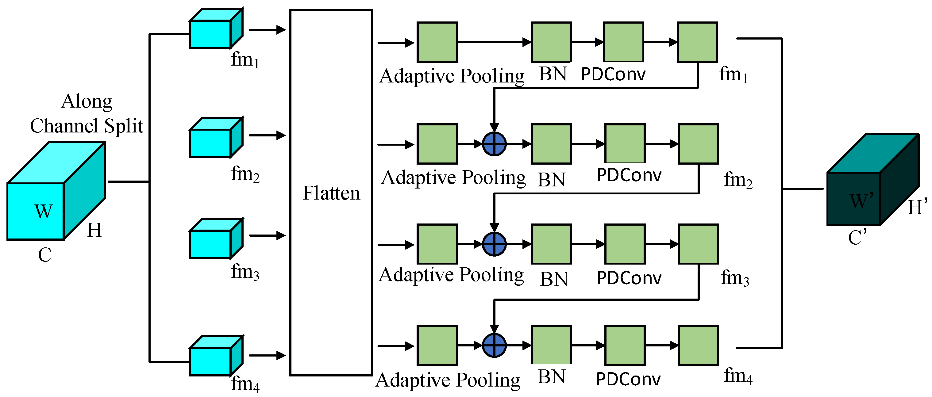
3.3.1. Backbone Network Model

To improve the accuracy and speed of SSD, it is necessary to integrate multi-scale features, and the model structure should be streamlined with fewer parameters. We designed a multi-scale feature fusion network structure based on Lie Group manifold space, as shown in Figure 3. Firstly, we map the data samples (including the support sample set and query sample set) onto the Lie Group manifold space. Subsequently, the model adopted 5 extraction stages, and the specific operations in each stage are shown in Figure 4.

Specifically, the data samples are first processed through batch normalization layers (BN). In the previous research results [48,49,50], we found that inserting BN layers before the convolution operations can effectively accelerate the convergence speed of the model, reduce the internal covariate shifts, and standardize sample features. As shown in Figure 4, we adopted multi-scale feature learning. Firstly, we divide the feature map into four partitions along the channel and convert it into a two-dimensional array feature through the flattening operation. This can effectively represent and calculate the correlation between each feature pixel. Unlike traditional models that use max pooling and average pooling, we utilize depthwise convolution for adaptive pooling and leverage BN and parallel dilated convolution operations. It should be noted that the SSD model needs to satisfy the real-time requirements of detection, and the number of model parameters should be as small as possible. Previous studies have shown that larger kernel convolution has a larger receptive field and can effectively extract features from samples. However, such convolutions often contain a larger number of parameters, which reduces the computational performance of the model and cannot satisfy the requirements of real-time detection. Therefore, we did not leverage traditional larger kernel convolution operations, but instead adopted parallel dilated convolution operations, effectively reducing the number of feature parameters while having a larger receptive field, as shown in

Table 1. Comparison of parameters between traditional convolution and parallel dilated convolution. Under the same size of convolution kernels, parallel dilated convolution has fewer parameters compared to traditional convolution. In addition, compared to traditional convolution, increasing the receptive field also reduces the number of parameters.

Convolution	Kernel Size	Input Channel	Output Channel	Layer	Parameters	Total (M)
Traditional	$3\times 3$	512	512	Conv1	$512\times 512\times 3\times 3=$ 2,359,296	7,077,888 $\approx 7.08$
				Conv2	$512\times 512\times 3\times 3=$ 2,359,296
				Conv3	$512\times 512\times 3\times 3=$ 2,359,296
	$5\times 5$	512	512	Conv1	$512\times 512\times 5\times 5=$ 6,553,600	19,600,800 $\approx 19.6$
				Conv2	$512\times 512\times 5\times 5=$ 6,553,600
				Conv3	$512\times 512\times 5\times 5=$ 6,553,600
Parallel	$5\times 5$	512	512	Conv1	$512\times 512\times 5\times 5=$ 6,553,600	6,553,600 $\approx 6.55$
				Conv2
				Conv3

.

Then, we add the above-obtained feature map to the second partition, merge it with the feature map of the second partition, perform the same operation as above, and repeat this process. The final feature map is obtained by fusing the feature maps of four partitions. In this process, we adopted the reuse of feature maps and enhanced the interaction of feature information between different channel partitions through this approach. Compared to the parallel branch structure used in traditional models, our method can achieve feature extraction at multiple scales and expand the receptive field. For example, the model utilizes two cascaded $3\times 3$ convolution operations. The receptive field of the first convolution is $3\times 3$ (i.e., 9 values in the feature map), and when the stride size is 1, the actual receptive field of the second convolution is $5\times 5$ (i.e., 25 values in the feature map). Using the same receptive field can obtain a larger receptive field, which can capture finer-grained features. This is in line with the general requirements of defect object detection [51].

3.3.2. Attention Mechanism Based on Intrinsic Mean in Lie Group Manifold Space

Different from the traditional model utilizing convolution operation to reduce the number of model parameters and the complexity of the model, and inspired by previous research [52], we propose an attention mechanism based on the intrinsic mean in Lie Group manifold space, which adopts a parallel computing mode, including channel attention and spatial attention. Channel suppression or enhancement occurs through the dynamic allocation of weights in the feature channel, so that the detection model focuses on task-critical information; this makes the feature map contain richer, more comprehensive, and more discriminative features and can effectively improve the robustness of detection in complex scenarios.

In the channel attention mechanism, we treat each channel as a feature detector and enhance or suppress different channels through relevant operations. Specifically, for the feature map $X\in R^{W\times H\times C}$ obtained in the previous stage, where W, H, and C represent width, height, and channel respectively, we firstly calculate their corresponding intrinsic mean in the Lie Group manifold space and form a vector $\overrightarrow{V}\in R^{1\times 1\times C}$ ($\overrightarrow{V}=[{\overrightarrow{v}}_1,{\overrightarrow{v}}_2,\cdots ,{\overrightarrow{v}}_C]$). It should be noted that we did not use the traditional mean mainly because in our previous research [53,54], we found that compared to the traditional mean, the intrinsic mean in the Lie Group manifold space can better reflect the essential characteristics of the data sample, and it is simple to calculate and has lower feature dimensions, which can better satisfy the needs of real-time detection. The calculation of intrinsic mean and covariance in Lie Group manifold space is as follows:

$${\overline{\mu }}_{ch}=exp({\displaystyle \frac{1}{C}}\sum _{i=1}^{C}lo{g}_2{\overrightarrow{v}}_i)$$

(1)

$$C_{ch}={\displaystyle \frac{1}{C-1}}\sum _{i=1}^C({\overrightarrow{v}}_i-{\overline{\mu }}_{ch})$$

(2)

where ${\overline{\mu }}_{ch}$ and $C_{ch}$ denote the intrinsic mean and its corresponding covariance in the Lie Group manifold space on the channel dimension, and are logarithmic operations based on base 2. Suppose that ${\overrightarrow{V}}^{\prime }\in R^{1\times 1\times C}$ (${\overrightarrow{V}}^{\prime }=[{\overrightarrow{v}}_1^{\prime },{\overrightarrow{v}}_2^{\prime },\cdots ,{\overrightarrow{v}}_C^{\prime }]$), where ${\overrightarrow{v}}_i$ is the $i^{th}$ element in ${\overrightarrow{V}}^{\prime }$ and ${\overrightarrow{v}}_i^{\prime }={({\overrightarrow{v}}_i-{\overline{\mu }}_{ch})}^2$. The maximum and minimum values in ${\overrightarrow{V}}^{\prime }$ are denoted by ${\overrightarrow{v}}_{max}^{\prime }$ and ${\overrightarrow{v}}_{min}^{\prime }$, respectively, and can be obtained by the following calculation:

$$w_{ch}^i={\displaystyle \frac{{\overrightarrow{v}}_i^{\prime }}{{\overrightarrow{v}}_{max}^{\prime }-{\overrightarrow{v}}_{min}^{\prime }}}\times C_{ch},i\in [1,2,\cdots ,C]$$

(3)

where $W_{ch}=[w_{ch}^1,w_{ch}^2,\cdots ,w_{ch}^C]$. Finally, utilize the Lie Group sigmoid activation function to operate on it and obtain the feature weight values for each channel.

Figure 5 shows the operation process of the channel attention mechanism. Calculate the intrinsic mean and corresponding Lie Group covariance of the feature vector in the Lie Group manifold space, and obtain the final channel attention weight through the Lie Group sigmoid activation function. From Figure 5, we can observe that channels that are close to the intrinsic mean in the Lie Group manifold space are suppressed, and vice versa is strengthened.

In the spatial attention mechanism, similar to the above operations, calculate the intrinsic mean and covariance in the Lie Group manifold space of feature map $X\in R^{W\times H\times C}$, and $\overline{U}\in R^{H\times W\times 1}$ (${\overline{u}}_{ij}\in \overline{U}$), as follows:

$${\overline{\mu }}_{sp}=exp\left({\displaystyle \frac{1}{H\times W}}\sum _{i=1}^H\sum _{j=1}^{W}lo{g}_2{\overline{u}}_{ij}\right)$$

(4)

$$C_{sp}={\displaystyle \frac{1}{H\times W-1}}\sum _{i=1}^H\sum _{j=1}^W({\overline{u}}_{ij}-{\overline{\mu }}_{sp})$$

(5)

where ${\overline{\mu }}_{sp}$ and $C_{sp}$ denote the intrinsic mean and its corresponding covariance in the Lie Group manifold space on the spatial dimension, respectively. Suppose that ${\overline{U}}^{\prime }\in R^{H\times W\times 1}$, where ${\overline{u}}_{ij}^{\prime }$ is an element in ${\overline{U}}^{\prime }$ and ${\overline{u}}_{ij}^{\prime }={({\overline{u}}_{ij}-{\overline{\mu }}_{sp})}^2$. Similarly, ${\overline{u}}_{max}^{\prime }$ and ${\overline{u}}_{min}^{\prime }$ represent the maximum and minimum values in ${\overline{U}}^{\prime }$, $\overline{W}\in R^{H\times W\times 1}$ represents the matrix, and ${\overline{w}}_{ij}^{\prime }$ represents the elements, which can be obtained by the following calculation:

$$w_{ij}^{sp}={\displaystyle \frac{{\overline{u}}_{ij}^{\prime }}{{\overline{u}}_{max}^{\prime }-{\overline{u}}_{min}^{\prime }}}\times C_{sp},i\in [1,2,\cdots ,H],j\in [1,2,\cdots ,W]$$

(6)

Finally, utilize the Lie Group sigmoid activation function to operate on it and obtain the feature weight values for spatial dimension $W_{sp}$.

Figure 6 shows the operation process of the spatial attention mechanism. Similar to the channel attention mechanism, we can observe that regions that deviate from the intrinsic mean in the Lie Group manifold space are strengthened, and vice versa, they are weakened.

After applying the above operation for feature map $X\in R^{W\times H\times C}$, corresponding spatial attention weights and channel attention weights were obtained. Then, we multiply the two attention weights mentioned above to obtain the final attention weights and utilize residual connections to capture finer features. The specific operations are as follows:

$$X^{\prime }=(W_{ch}\otimes W_{sp})\oplus X$$

(7)

where $W_{ch}$ and $W_{sp}$ represent the channel attention weight and spatial attention weight, ⊗ represents element-wise multiply, and ⊕ represents element-wise sum.

3.4. Intrinsic Mean Feature Detector in Lie Group Manifold Space

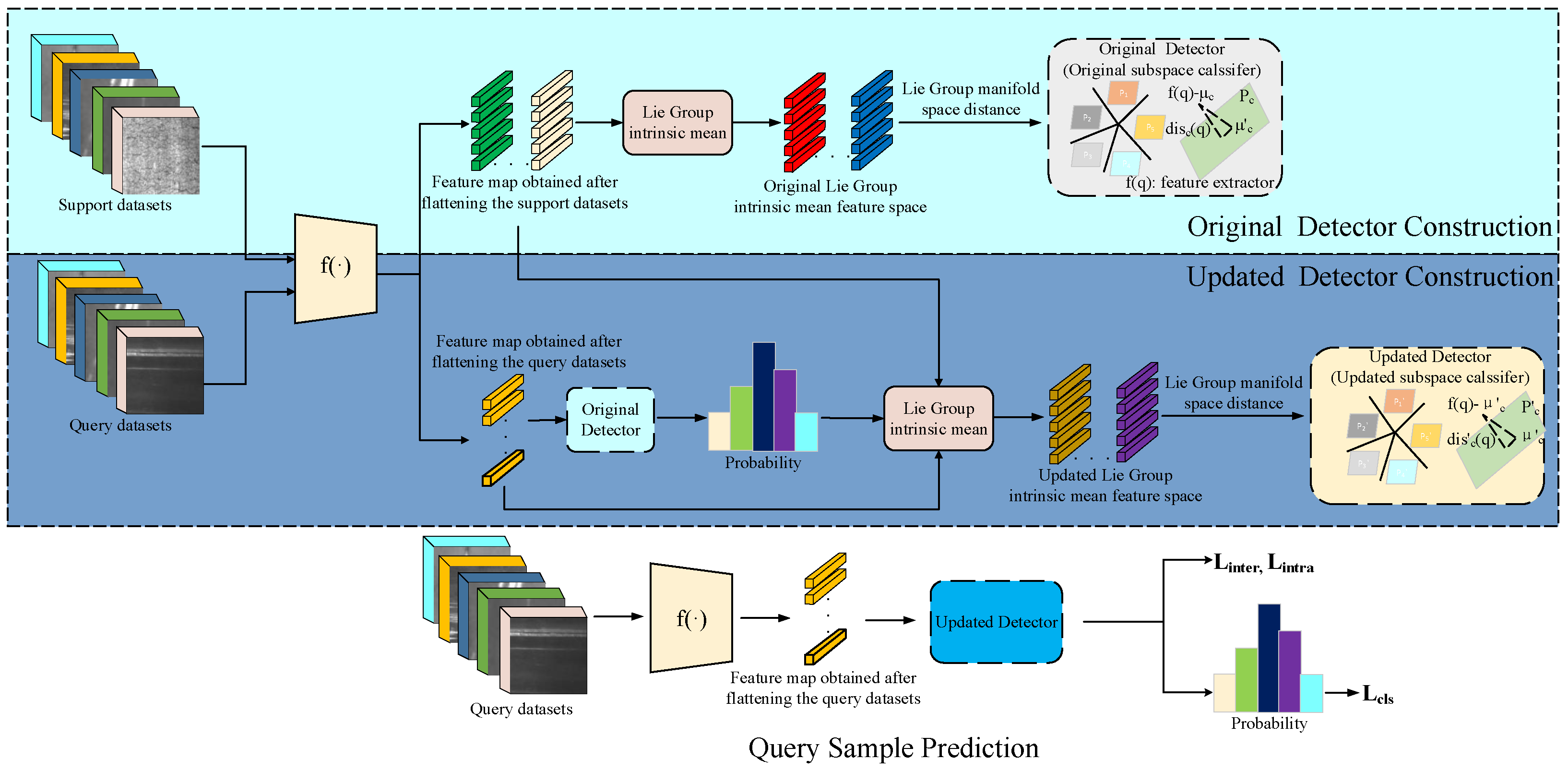
3.4.1. Methodology Overview

The framework of the intrinsic mean feature detector in the Lie Group manifold space is shown in Figure 7. Firstly, flatten the feature maps extracted from the above SSD framework, which is equivalent to mapping the samples to a higher-dimensional space, which is beneficial for improving the accuracy of defect detection. Then, we utilize methods such as intrinsic mean within the Lie Group manifold space to construct the original intrinsic mean feature detector within the Lie Group manifold space. This detector is used to predict the probability of the defect category that the query data sample belongs to. Finally, based on the above probabilities, the intrinsic mean feature detector in the original Lie Group manifold space is updated by combining the support dataset and query dataset to obtain the updated intrinsic mean feature detector in the Lie Group manifold space. The updated intrinsic mean feature detector is then used to predict the test samples. To improve the speed and accuracy of model detection, we adopt the episode-based approach [55] during the training process, which continuously updates and accumulates knowledge to predict test samples. In addition, we also use a novel loss function aimed at further improving the accuracy of defect detection.

3.4.2. Problem Definition

Since there are fewer defect data samples in actual production, our goal is to utilize these fewer defect data samples for defect detection of new data samples. In this study, we divide the dataset $DS$ into $D{S}_{train}$, $D{S}_{val}$, and $D{S}_{test}$ with $D{S}_{train}\cap D{S}_{val}\cap D{S}_{test}=\varnothing$. We also construct a series of other learning tasks, each containing T different categories. Select $S+Q$ data samples for each category, where S represents the support data set $S=\{(x_{11},y_{11}),(x_{12},y_{12}),\cdots ,(x_{TS},y_{TS})\}$, Q represents the query data set $Q=\{q_1,q_2,\cdots ,q_{T\times Q}\}$, $x_{ij}$ represents the $j^{th}$ data sample of the $i^{th}$ category, $y_{ij}$ represents the label of the corresponding data sample, $q_i$ represents the $i^{th}$ query sample, and satisfies $S\cap Q=\varnothing$.

3.4.3. Original Lie Group Manifold Space Intrinsic Mean Feature Detector

For the supporting data set $S={\left\{(x_i,y_i)\right\}}_{i=1}^{T\times S}$, we construct the original Lie Group manifold space intrinsic mean feature detector. Firstly, we calculate the intrinsic mean within the Lie Group manifold space of class c as follows.

$${\overline{\mu }}_c={\displaystyle \frac{1}{S}}\sum _{x_j\in S_c}f\left(x_j\right)$$

(8)

where $f(·)$ represents the previously obtained feature map and $S_c={\left\{(x_j,y_j)\right\}}_{j=1}^S$ represents the supporting data samples belonging to category c. Next, construct the intrinsic mean feature space within the original Lie Group for each category c, as shown below:

$${\dot{X}}_c=[f\left(x_{c1}\right)-{\overline{\mu }}_c,f\left(x_{c2}\right)-{\overline{\mu }}_c,\cdots ,f\left(x_{cS}\right)-{\overline{\mu }}_c]$$

(9)

Since Euclidean spatial distance directly calculates the straight-line distance between two data samples and does not fully consider the actual scene of the samples, as shown in Figure 8, Euclidean spatial distance cannot truly represent the actual distance between two samples. Therefore, based on our previous research [24,49,50,56], we adopt the Lie Group manifold space distance to calculate and analyze the actual distance from each query sample to each subclass space. The basic idea of the intrinsic mean feature detector in the original Lie Group manifold space is to find the shortest Lie Group manifold space distance from the test data sample to its subclass space. For the query data sample $q_i$, calculate the spatial distance of the Lie Group as follows:

$$di{s}_c\left(q_i\right)=∥logf\left(q_i\right)-log{\overline{\mu }}_c∥$$

(10)

where $∥·∥$ represents the Frobenius function, i.e.,: $∥X∥=\sqrt{{\sum }_{i=1}^m{\sum }_{j=1}^n{\left|x_{ij}\right|}^2}$. For details about other Lie Group machine learning, please refer to [53,54,57].

Based on the obtained Lie Group manifold space distance, utilize the softmax function to predict the probability that the query sample $q_i$ belongs to a certain class c of defects, which is calculated as follows:

$$p(y=c|q_i)={\displaystyle \frac{exp(-di{s}_c\left(q_i\right))}{{\sum }_{c^{\prime }}exp(-di{s}_c\left(q_i\right))}}$$

(11)

where $c^{\prime }\in \{0,1,\cdots ,T-1\}$ represents the category in each learning task.

3.4.4. Updated Lie Group Manifold Space Intrinsic Mean Feature Detector

On the basis of the above, we added sample features from the query dataset to update and refine the intrinsic mean feature detector in the original Lie Group manifold space, and leveraged the intrinsic mean feature detector in the original Lie Group manifold space to complete the final defect detection, further improving the accuracy of defect detection.

For a certain query sample $q_i$, we first utilize the intrinsic mean feature detector in the original Lie Group manifold space to predict its probability of belonging to a certain type of defect. The calculation is as follows:

$$p_{c,i}={\displaystyle \frac{exp(-di{s}_c\left(q_i\right))}{{\sum }_{c^{\prime }}exp(-di{s}_c\left(q_i\right))}}$$

(12)

Then, utilize the probability obtained above to update the original model and calculate as follows:

$${\overline{\mu }}_c^{\prime }={\displaystyle \frac{{\sum }_{x_j\in S_c}f\left(x_j\right)+{\sum }_i{p}_{c,i}f\left(q_i\right)}{S+{\sum }_i{p}_{c,i}}}$$

(13)

where ${\overline{\mu }}_c^{\prime }$ represents the updated Lie Group intrinsic mean. In addition, we construct the updated intrinsic mean feature space in the Lie Group manifold space for each category c, as follows:

$${\ddot{X}}_c=[f\left(x_{c1}\right)-{\overline{\mu }}_c^{\prime },f\left(x_{c2}\right)-{\overline{\mu }}_c^{\prime },\cdots ,f\left(x_{cS}\right)-{\overline{\mu }}_c^{\prime }]$$

(14)

Through the above operations, we have updated the new Lie Group intrinsic mean feature space for each defect category. The new Lie Group spatial distance calculation is as follows:

$$di{s}_c^{\prime }\left(q_i\right)=∥logf\left(q_i\right)-log{\overline{\mu }}_c^{\prime }∥$$

(15)

Next, utilize the softmax function to predict the probability that the query sample belongs to a certain type of defect, and calculate as follows:

$$p^{\prime }(y=c|q_i)={\displaystyle \frac{exp(-di{s}_c^{\prime }\left(q_i\right))}{{\sum }_{c^{\prime }}exp(-di{s}_c^{\prime }\left(q_i\right))}}$$

(16)

3.4.5. Loss Function

To improve the accuracy of defect detection, we add the loss function, which contains three parts, namely, the classification loss function, the loss function between different defect categories, and the loss function within the defect categories.

In the classification loss function, the main goal is to correctly detect and identify as many defect detection samples as possible, so the cross-entropy loss function is adopted as follows:

$$Los{s}_{cls}=-{\displaystyle \frac{1}{T\times Q}}\sum _{q=1}^{T\times Q}log\left(p_{c,q}\right)$$

(17)

Due to the confusion between different categories of defect samples, we add a loss function between different defect categories. Specifically, we take two different types of defect datasets as examples, whose Lie Group intrinsic mean feature spaces are ${\ddot{X}}_1$ and ${\ddot{X}}_2$, respectively. The Lie Group spatial distance of these two types of defects is calculated as follows:

$$d({\ddot{X}}_1,{\ddot{X}}_2)=∥\mathrm{l}\mathrm{o}\mathrm{g}({\ddot{X}}_1^{-1}{\ddot{X}}_2)∥$$

(18)

where $∥·∥$ represents Frobenius function.

Our goal is to maximize the above Lie Group spatial distance, thus obtaining the loss function between different defect categories, represented as follows:

$$Los{s}_{inter}={\displaystyle \frac{2}{T\times (T-1)}}\sum _{i=1}^T\sum _{j=1}^T∥\mathrm{l}\mathrm{o}\mathrm{g}({\ddot{X}}_i^{-1}{\ddot{X}}_j)∥$$

(19)

where T represents the number of classes in each task.

To reduce the intraclass Lie Group intrinsic mean variance of test data samples to their corresponding Lie Group intrinsic mean feature space, so that the Lie Group intrinsic mean feature space of defect samples belonging to the same type has greater similarity, we use the loss function within the defect class, which is expressed as follows:

$$Los{s}_{intra}=1-{\displaystyle \frac{1}{T\times Q}}\sum _{i=1}^{T\times Q}cos<q_i,{\overline{\mu }}_c^{\prime }>$$

(20)

where $cos<·>$ denotes the cosine similarity.

Combining the above three parts, we obtain the final loss function:

$$Loss=Los{s}_{cls}+\alpha Los{s}_{inter}+\beta Los{s}_{intra}$$

(21)

where $\alpha$ and $\beta$ represent hyperparameters, respectively, we conduct a large number of experiments, and a better detection performance can be achieved when $\alpha =0.426$ and $\beta =0.574$.

4. Experiments

To validate the effectiveness of our model, we conduct extensive experiments on three publicly available and challenging datasets. Firstly, we introduce some details of the dataset and experiments. Then, we select some classic and state-of-the-art models to compare to our model. Finally, the effectiveness of the crucial components of our model is verified through ablation experiments.

4.1. Datasets and Implementation Details

We select datasets from real industrial production environments, namely the NEU-DET dataset [3], the steel surface defect dataset [3], and the railway tracks dataset [58]. To verify the robustness and generalization of the model, we divided the dataset into different proportions, as shown in

Table 2. Details of the three Datasets.

Datasets	Class	Image Number	Image per-Class	Training Ratio and Validation Ratio
Steel surface	10	2294	100∼300	50%, 30%
Railway tracks	2	195	85∼100	50%, 30%
NEU-DET	6	1800	300	50%, 30%

. Specifically, the training dataset is mainly utilized to train the model, the validation dataset is mainly utilized to select the optimal model, and the test dataset is utilized to evaluate the performance of the model.

For a fair comparison, all experiments in this study were conducted under the same training parameters and experimental environment, as shown in

Table 3. Experimental environment parameters.

Item	Content
Processor	Intel Core i7-4700 CPU with 2.70 GHz $\times 12$ (Santa Clara, CA, USA)
Memory	32 GB (Kingston: Fountain Valley, CA, USA—Headquarters)
Operating system	Windows 7 Pro (Microsoft: Redmond, DC, USA)
Hard disk	1 T (Western Digital: San Jose, CA, USA—Headquarters)
Software	Matlab 2019a (MathWorks, Netik, MA, USA)
GPU	Nvidia Titan-X $\times 2$ (NVIDIA, Santa Clara, CA, USA)
PyTorch	v1.1 (Meta AI, Menlo Park, CA, USA)
Batch size	120
Learning rate	0.00326∼0.15
Momentum	0.863
Weight decay	0.000386
Antenna gain	5 dBi
Noise power	${10}^{-3}$ W
Transmission power	1.0∼1.5 W
Wireless bandwidth	20 Mhz

. To verify the feasibility and robustness of the model, we did not utilize any data augmentation methods, and the experiments were performed according to the authors’ default settings.

4.2. Experimental Results and Comparison

We select the state-of-the-art detection methods and several popular attention mechanisms (such as SE and CBAM) to compare with our model. The main evaluation metrics include accuracy (ACC), F1, Precision, Recall, number of model parameters, and floating point operations (FLOPs). These indicators are mainly used to measure the accuracy of the detection model, the size of the model, the computational performance, and other related important indicators.

4.2.1. Results and Comparison of Steel Surface Defect Dataset

Table 4. Performance comparison of 17 models on the steel surface defect dataset.

Methods	Param (M)	FLOPs (G)	Acc (%)	F1 (%)	Prec (%)	Recall (%)
CenterNet [3]	$31.6$	$119.3$	$72.16$	$58.36$	$60.43$	$59.15$
CenterNet + SE [3]	$32.3$	$124.6$	$72.38$	$63.55$	$65.31$	$64.38$
CenterNet + CBAM [3]	$32.3$	$124.6$	$72.59$	$59.57$	$61.15$	$60.33$
CenterNet + SimAM [3]	$31.6$	$125.2$	$72.57$	$62.07$	$63.07$	$62.02$
CenterNet + HFAM [3]	$31.6$	$125.2$	$72.77$	$63.46$	$65.27$	$64.35$
Faster R-CNN [3]	$35.9$	$129.3$	$73.19$	$63.57$	$66.15$	$64.67$
Faster R-CNN + SE [3]	$36.1$	$129.9$	$73.33$	$63.69$	$65.73$	$64.72$
Faster R-CNN + CBAM [3]	$36.2$	$129.9$	$73.55$	$63.77$	$66.17$	$64.86$
Faster R-CNN + SimAM [3]	$35.9$	$129.2$	$73.57$	$64.25$	$66.36$	$65.21$
Faster R-CNN + HFAM [3]	$35.9$	$129.2$	$74.55$	$64.53$	$67.17$	$65.72$
SSD [3]	$135.7$	$38.7$	$71.75$	$54.56$	$56.63$	$56.28$
YOLO v5S [3]	$7.3$	$16.6$	$85.72$	$63.25$	$65.41$	$64.33$
YOLO v9S [59]	$7.3$	$26.6$	$86.25$	$66.37$	$68.51$	$66.52$
YOLO v9M [59]	$20.2$	$76.9$	$86.72$	$71.37$	$74.46$	$73.27$
YOLO v9C [59]	$25.6$	$102.9$	$86.89$	$74.25$	$77.31$	$76.55$
YOLO v9E [59]	$58.2$	$192.7$	$87.76$	$74.57$	$78.26$	$76.87$
RTMEC [3]	$12.9$	$15.8$	$88.79$	$75.69$	$79.13$	$78.35$
Proposed	$6.5$	$10.7$	$89.87$	$79.37$	$82.65$	$81.23$

offers the experimental results of different models and attention mechanisms. From the experimental results, we can find that:

• Under the same training ratio, our proposed model significantly improves the accuracy of defect detection compared to other models. Specifically, our model improves 17.1%, 16.32%, and 3.62% (89.87% vs 72.77%, 89.87% vs 73.55%, and 89.87% vs 86.25%) compared to CenterNet + HFAM [3], Faster R-CNN + CBAM [3], and YOLO v9S [59]. (The core improvement of YOLO v9S lies in dynamic parameter adjustment and hardware adaptation optimization, which improves the adaptability and deployment efficiency of the model in complex scenarios by flexibly controlling the number of channels, module depth, and memory alignment), respectively. Some models (such as CenterNet [3] and Faster R-CNN [3]) are detected by combining attention mechanism, and experimental results show that these models have higher detection accuracy compared to other models. In contrast, we adopt multi-scale fusion features, which can extract finer feature maps.
• Our proposed model adopts the attention mechanism based on the intrinsic mean in the Lie Group manifold space and achieves the highest detection accuracy under the same training ratio. Specifically, compared to the CBAM attention mechanism, our model improves 16.32%.
• In terms of the number of parameters and FLOPs, our model has certain advantages over other models. For example, compared to YOLO v5S [3], our model parameters have decreased by $0.8M$. From the experimental results, we can find that our model has better computational performance and fewer parameters. Compared with other models, it can better satisfy actual production needs.

4.2.2. Results and Comparison of Railway Tracks Dataset

Table 5. Performance comparison of 17 models on the railway tracks dataset.

Methods	Param (M)	FLOPs (G)	Acc (%)	F1 (%)	Prec (%)	Recall (%)
CenterNet [3]	$30.6$	$116.2$	$77.32$	$60.22$	$62.73$	$60.15$
CenterNet + SE [3]	$31.2$	$121.3$	$77.56$	$61.34$	$63.27$	$60.44$
CenterNet + CBAM [3]	$31.3$	$121.3$	$77.73$	$61.67$	$64.36$	$62.19$
CenterNet + SimAM [3]	$30.6$	$116.3$	$77.21$	$66.51$	$69.33$	$64.29$
CenterNet + HFAM [3]	$30.6$	$116.3$	$77.92$	$62.37$	$64.13$	$62.67$
Faster R-CNN [3]	$35.6$	$127.2$	$75.26$	$56.71$	$59.15$	$58.63$
Faster R-CNN + SE [3]	$35.7$	$129.2$	$75.36$	$62.47$	$59.82$	$65.39$
Faster R-CNN + CBAM [3]	$35.8$	$129.5$	$75.47$	$61.39$	$64.22$	$60.29$
Faster R-CNN + SimAM [3]	$35.6$	$127.2$	$74.13$	$59.77$	$61.26$	$60.37$
Faster R-CNN + HFAM [3]	$35.6$	$127.2$	$75.79$	$61.21$	$63.34$	$62.45$
SSD [3]	$134.3$	$37.5$	$72.82$	$53.76$	$56.52$	$55.16$
YOLO v5S [3]	$7.2$	$16.5$	$87.73$	$65.42$	$68.37$	$66.59$
YOLO v9S [59]	$7.2$	$26.7$	$88.31$	$67.59$	$69.67$	$62.45$
YOLO v9M [59]	$20.1$	$76.8$	$89.53$	$74.22$	$78.37$	$76.58$
YOLO v9C [59]	$25.5$	$102.8$	$89.75$	$75.37$	$77.46$	$76.51$
YOLO v9E [59]	$58.1$	$192.5$	$89.96$	$76.63$	$79.25$	$77.42$
RTMEC [3]	$12.7$	$15.6$	$91.23$	$78.37$	$79.35$	$77.51$
Proposed	$6.5$	$10.6$	$92.41$	$78.57$	$79.77$	$77.65$

reports the experimental results on the railway tracks dataset. From the experimental results, we find that:

• We utilize multi-scale feature fusion to enhance the feature representation ability of the model at different scales. With the training ratio of 50%, the detection accuracy reaches 92.41%, which is 15.09%, 17.15%, and 19.59% higher than the baseline models CenterNet [3], Faster R-CNN [3], and SSD [3] without attention mechanism, respectively. Compared with CenteNet + HFAM [3], YOLO v9C [59], and RTMEC [3], the proposed algorith/ov9, and RTMEC [3], the proposed algorithm improves the detection accuracy by 14.49%, 2.66%, and 1.18%, respectively.
• We find that in most cases, the detection accuracy of the model with attention mechanism is higher than that of the model without attention mechanism. For example, the detection accuracy of Faster R-CNN + HFAM [3] is improved by 0.53% compared to Faster R-CNN [3]. However, in some cases, the introduction of the attention mechanism even reduces the model detection accuracy, indicating that the attention mechanism damages the performance of the model, such as Faster R-CNN + SimAM [3].
• In terms of F1 and Recall, our model improves 0.2% and 0.14%, respectively, compared with RTMEC [3]. The experimental results once again reflect the comprehensiveness of our model. Similar to the HFAM and SimAM attention mechanisms, our proposed attention mechanism based on the intrinsic mean in the Lie Group manifold space does not increase the number of parameters of the model. It should be noted that, compared with other attention mechanisms (such as CBAM and SimAM), we do not utilize hyperparameters, which is more conducive to the deployment of the model in actual production.

4.2.3. Results and Comparison of the NEU-DET Dataset

To further validate the effectiveness of our model, we conducted a large number of experiments on the NEU-DET dataset, and the experimental results are shown in

Table 6. Performance comparison of 17 models on the NEU-DET Dataset.

Methods	Param (M)	FLOPs (G)	Acc (%)	F1 (%)	Prec (%)	Recall (%)
CenterNet [3]	$30.6$	$116.2$	$76.37$	$58.63$	$61.65$	$59.53$
CenterNet + SE [3]	$31.2$	$121.3$	$76.49$	$58.86$	$62.07$	$61.35$
CenterNet + CBAM [3]	$31.3$	$121.3$	$76.65$	$59.22$	$63.25$	$61.63$
CenterNet + SimAM [3]	$30.6$	$116.3$	$76.59$	$58.92$	$62.36$	$61.53$
CenterNet + HFAM [3]	$30.6$	$116.3$	$77.25$	$63.51$	$66.21$	$64.53$
Faster R-CNN [3]	$35.6$	$127.2$	$74.67$	$56.87$	$59.38$	$58.77$
Faster R-CNN + SE [3]	$35.7$	$129.2$	$74.78$	$60.35$	$63.22$	$61.56$
Faster R-CNN + CBAM [3]	$35.8$	$129.5$	$74.83$	$62.55$	$65.17$	$64.37$
Faster R-CNN + SimAM [3]	$35.6$	$127.2$	$74.56$	$60.42$	$64.37$	$62.59$
Faster R-CNN + HFAM [3]	$35.6$	$127.2$	$75.45$	$63.56$	$67.28$	$66.36$
SSD [3]	$134.3$	$37.5$	$71.77$	$68.32$	$70.38$	$69.51$
YOLO v5S [3]	$7.2$	$16.5$	$79.32$	$65.66$	$69.23$	$67.83$
YOLO v9S [59]	$7.2$	$26.7$	$79.41$	$66.63$	$69.85$	$67.37$
YOLO v9M [59]	$20.1$	$76.8$	$79.52$	$64.57$	$65.62$	$64.33$
YOLO v9C [59]	$25.5$	$102.8$	$79.65$	$68.75$	$72.81$	$71.07$
YOLO v9E [59]	$58.1$	$192.5$	$79.78$	$65.92$	$71.59$	$70.36$
RTMEC [3]	$12.7$	$15.6$	$81.76$	$77.29$	$79.67$	$78.35$
Proposed	$6.5$	$10.6$	$82.69$	$78.61$	$79.91$	$78.76$

. From Table 6, we find that:

• Our model performs the best, consistent with the experimental results of the two datasets mentioned above. Specifically, our model achieves a defect detection accuracy of 82.69%, which is superior to other models. Compared with YOLO v5S [3], Faster R-CNN + HFAM [3], and RTMEC [3], the detection accuracy has been improved by 3.37%, 8.13%, and 0.93%, respectively. In addition to the advantage in detection accuracy, our model also demonstrates certain advantages in F1 and Recall metrics.
• The experimental results show that in the case of the same training ratio of data samples, compared with other attention mechanisms, our proposed attention mechanism based on the intrinsic mean in the Lie Group manifold space can help the model improve detection accuracy without increasing the number of model parameters and computational complexity. This is crucial for deployment in real production environments.
• In terms of the number of model parameters and computational performance, the experimental results further verify the superiority of our proposed model. From the experimental results, we find that in SimAM, HFAM, and our attention mechanism, the number of parameters of the model is not increased. In addition, we have advantages in detection accuracy and the number of parameters, and our method, like HFAM, does not require extensive experimentation to identify hyperparameters, which is a significant advantage for deploying the model on the edge server.

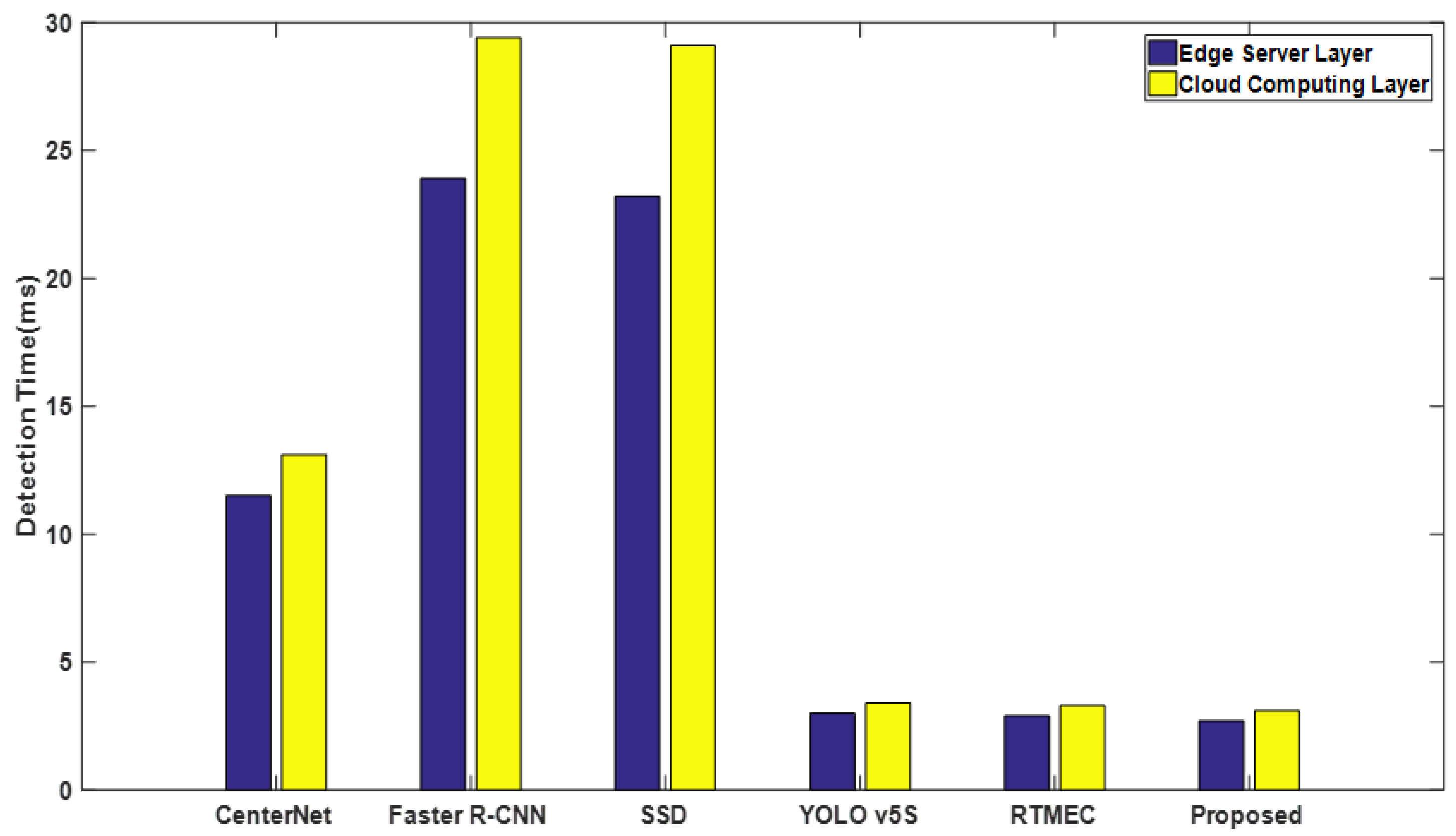
4.2.4. Comparison of Real-Time Performance of Different Detection Models

To satisfy the needs of actual production, in this section, we analyze the real-time performance of the defect detection model. Specifically, we select a variety of defect detection models, such as CenterNet, Faster-RCNN, SSD, and YOLO v5s, and deploy them on the edge server layer and the cloud computing layer for simulation experiments. The parameters of the edge server and cloud computing server are shown in

Table 7. Parameter information about the cloud computing server and edge server.

Item	GeForce RTX 3090	GeForce RTX 2080 Ti
CUDA Cores	8704	2944
GPU Memory	24 GB	12 GB
Anacoda Version	$\mathrm{4.8.2}$	$\mathrm{4.8.2}$
CentOS Linux	$\mathrm{8.5.2111}$	$\mathrm{8.5.2111}$
CUDA Version	$11.6$	$11.4$
CuDNN Version	$\mathrm{8.2.1}$	$\mathrm{8.2.1}$
Driver Version	$510.47$	$470.86$
Enforced Power Limit	320 W	215 W

.

Table 8. Comparison of detection time and FPS performance of different defect detection models at edge server layer and cloud computing layer.

Model	Railway Racks				NEU-DET
	Detection Times on GPU 2080Ti (ms)	Detection Times on GPU 3090 (ms)	FPS on GPU 2080Ti (Hz)	FPS on GPU 3090 (Hz)	Detection Times on GPU 2080Ti (ms)	Detection Times on GPU 3090 (ms)	FPS on GPU 2080Ti (Hz)	FPS on GPU 3090 (Hz)
CenterNet [3]	11.7	10.4	89.3	96.2	13.1	11.5	71.37	79.76
Faster R-CNN [3]	27.5	23.8	37.7	46.6	29.4	23.9	11.8	14.9
SSD [3]	26.8	22.4	43.86	44.6	29.1	23.2	59.72	66.87
YOLO v5S [3]	2.7	2.4	384.6	416.7	3.4	3.0	133.7	148.2
RTMEC [3]	3.2	2.8	312.5	357.1	3.3	2.9	118.4	131.5
Proposed	2.5	2.1	387.2	419.2	3.1	2.7	119.7	151.6

and Figure 9 respectively report the detection delay of different models deployed at the edge server layer and cloud computing layer. From the experimental results, we can find that:

• Edge servers have significantly lower detection delay compared to the cloud computing layer. For example, Faster R-CNN [3] has a detection delay of $27.5$ ms on the edge servers and $23.8$ ms on the cloud computing layers, saving $3.7$ ms in detection delay. The detection delay of our model on the edge server is reduced by $0.4$ ms compared to the cloud computing layer. This is mainly because it takes more time and costs for the defect data samples to be transmitted from the IoT device layer to the cloud computing layer than to the edge service layer; that is, the transmission delay is caused by the longer transmission link, network bandwidth, force majeure, and other factors.
• Considering that in the actual production process, as the number of data sets collected by IoT devices continues to increase, the number of datasets sent to the cloud computing layer will also increase; the network may be congested, and the bandwidth of the network may be one of the bottleneck factors leading to low efficiency of defect detection. Therefore, from the above experimental results, it can be found that our model can effectively cope with the real-time requirements of tiny SSD.

4.3. Ablation Experiment

4.3.1. Impact of Different Modules on the Model

We evaluate the influence of different modules on the defect detection model. Taking the NEU-DET dataset as an example, we start with feature extraction, add the Lie Group intrinsic mean attention mechanism, Lie Group spatial distance, original Lie Group manifold space intrinsic mean feature detector, updated Lie Group manifold space intrinsic mean feature detector, and loss function, and finally obtain the final defect detection model. The experimental results are shown in

Table 9. Ablation experiment results of different modules in the NEU-DET dataset.

Component	Acc (%)	F1 (%)	Prec (%)	Recall (%)
Feature Extraction	77.23	53.27	61.17	53.67
Lie Group intrinsic mean attention mechanism	79.63	65.26	65.11	65.52
Lie Group spatial space	80.75	67.31	69.35	65.53
Original Model	80.93	69.67	72.35	68.37
Updated Model	82.69	78.61	79.97	78.76

. From Table 9, we find that after adding the Lie Group intrinsic mean attention mechanism, ACC and F1 are improved by $2.4\%$ and $11.99$, respectively. After adding Lie Group spatial distance, original Lie Group manifold space intrinsic mean feature detector, and updated Lie Group manifold space intrinsic mean feature detector to the model, ACC and F1 are improved by $3.06\%$ and $13.35$, respectively. The experimental results show that the added Lie Group spatial distance can effectively distinguish different types of defects, and the updated Lie Group manifold space intrinsic mean feature detector has better detection performance. The above combination achieves an ACC of 82.69%, a Recall of 78.76%, and an F1 of 78.61, which again validates the effectiveness of the individual modules.

4.3.2. Impact of Inserting Attention Mechanism at Different Stages on the Model

Table 10. Effects of different stages of inserting attention mechanisms on the model in the NEU-DET dataset. ✓ indicates that it has been used at this stage.

Methods	Stage1	Stage2	Stage3	Stage4	Stage5	ACC (%)	F1 (%)	Prec (%)	Recall (%)
Ours					✓	78.15	66.36	63.28	62.78
				✓	✓	79.33	68.47	69.86	67.62
			✓	✓	✓	80.46	70.52	68.16	66.73
		✓	✓	✓	✓	81.52	72.76	71.97	70.82
	✓	✓	✓	✓	✓	82.69	78.61	79.91	78.76

✓ indicates that it has been used at this stage.

reports the detection performance of the defect detection model with the spatial attention mechanism of Lie Group inserted at different stages. From the experimental results, we can find that the performance of only inserting it in the fifth stage is significantly lower than that of inserting it in the fourth and fifth stages simultaneously. The experimental results verify the effectiveness of the Lie Group spatial attention mechanism and also verify the necessity of inserting the Lie Group spatial attention mechanism in each stage of our proposed model, which can help the model better focus on the characteristics of the crucial regions in the defect sample and ignore the unimportant regions.

4.3.3. Impact of the Loss Function on the Model

In this article, we also investigate the influence of interclass similarity between defect samples of different types and the impact of the intraclass variance of defect samples within the same type on defect detection performance. Therefore, we analyze the impact of setting the loss function on defect detection performance. We conducted a series of experiments on the two datasets mentioned above, namely the railway tracks data and the NEU-DET dataset. In the experiments, the other modules of the defect detection model remained the same, and different loss functions were utilized; namely, the first group utilized the traditional cross-loss function, and the second group utilized our proposed loss function. The experimental results are shown in

Table 11. Performance comparison of models using different loss functions on Railway racks and NEU-DET data sets.

Loss Function	Railway Racks				NEU-DET
	Acc (%)	F1 (%)	Prec (%)	Recall (%)	Acc (%)	F1 (%)	Prec (%)	Recall (%)
Cross-Entopy Loss	90.36	78.39	78.68	76.41	80.97	77.39	77.67	76.82
Our Proposed Loss	92.41	78.57	79.77	77.65	82.69	78.61	79.91	78.76

. From the experimental results, we can find that the defect detection performance of the loss function proposed by us is better than that of the traditional loss function, and the loss function proposed by us achieves the best performance. Therefore, for defect detection tasks, our proposed loss function can effectively distinguish the similarity between different types of defect samples and the differences between samples of the same type of defect, thereby achieving better detection performance.

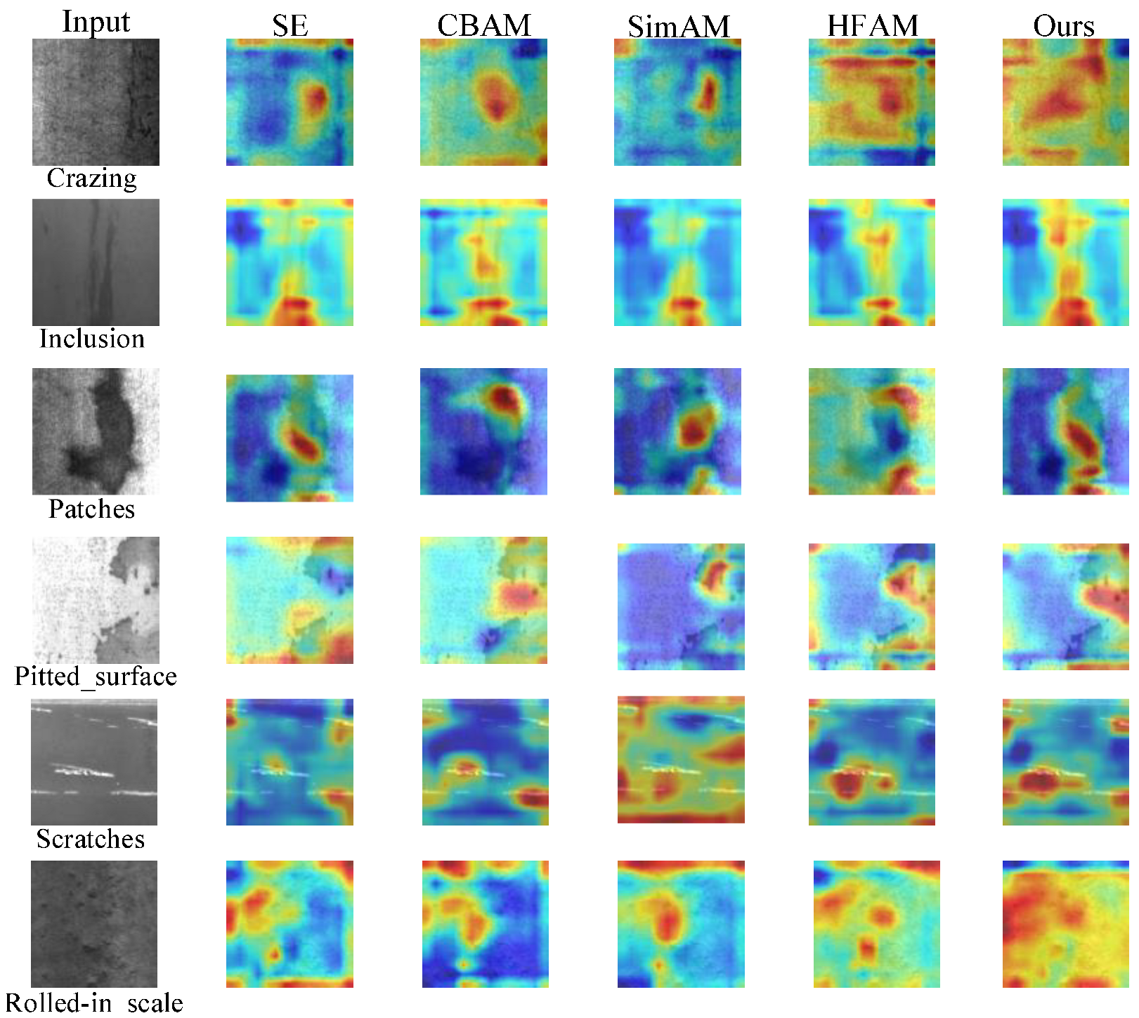
4.3.4. Visual Inspection of the Lie Group Manifold Space Attention Mechanism

To further illustrate that our proposed attention mechanism can effectively capture crucial feature information in defect data samples, we select several popular attention mechanisms (such as SE and CBAM) and compare them with our model. We apply the Grad-CAM [60] method to the NEU-DET dataset and reflect the crucial regions in the model in the form of heat maps. The experimental results are shown in Figure 10. From the experimental results, we can find that compared with other attention mechanisms, our proposed attention mechanism can capture more refined features focusing on crucial areas and major defect objects when processing complex data samples, so it can obtain more accurate features in crucial regions than other attention mechanisms. The experimental results once again verify that our proposed attention mechanism helps the model to capture more and finer discriminative features and pay more attention to defective regions in the dataset samples.

5. Conclusions

In this study, we propose a novel model for real-time SSD. We construct a more suitable and efficient model for improving the real-time detection of tiny surface defects. Since the Lie Group manifold space intrinsic feature space can more effectively represent the essential commonalities of different defect types, this model adopts the Lie Group manifold space intrinsic feature space as a metric for different defect types. We also consider the actual application scenario of the SSD model, which needs to satisfy the real-time, efficiency, and accuracy of defect detection. We propose an attention mechanism based on Lie Group manifold space, which is simple to calculate and easy to implement, does not contain any hyperparameters, and does not increase the number of parameters of the model. In particular, we first pre-train a Lie Group manifold space intrinsic mean feature detector (also known as the universal detector) with supporting data samples on the cloud computing layer, and then update the original Lie Group manifold space intrinsic mean feature detector according to the defect data samples captured by different IoT devices. The updated detector has a more accurate Lie Group intrinsic feature space and better defect detection performance. In addition, to further improve the performance of defect detection, we also propose a novel loss function, which fully considers the interclass similarity between defect samples of different types and the larger intraclass variance of defect samples of the same type. Extensive experiments are conducted on three public and challenging datasets. The experimental results show that our proposed model has great advantages in terms of defect detection accuracy, detection delay, and model computational performance.

References

1. Zhao, Z.; Zhang, H.; Wang, L.; Huang, H. A Multimodel Edge Computing Offloading Framework for Deep-Learning Application Based on Bayesian Optimization. IEEE Internet Things J. 2023, 10, 18387–18399. [Google Scholar] [CrossRef]
2. Al-Sarawi, S.; Anbar, M.; Abdullah, R.; Al Hawari, A.B. Internet of things market analysis forecasts, 2020–2030. In Proceedings of the 2020 Fourth World Conference on Smart Trends in Systems, Security and Sustainability (WorldS4), London, UK, 15–17 July 2020; pp. 449–453. [Google Scholar] [CrossRef]
3. Li, H.; Li, X.; Fan, Q.; Xiong, Q.; Wang, X.; Leung, V.C.M. Transfer learning for real-time surface defect detection with multi-access edge-cloud computing networks. IEEE Trans. Netw. Serv. Manag. 2024, 21, 310–323. [Google Scholar] [CrossRef]
4. Li, Z.; Duan, M.; Xiao, B.; Yang, S. A novel anomaly detection method for digital twin data using deconvolution operation with attention mechanism. IEEE Trans. Ind. Inform. 2022, 19, 7278–7286. [Google Scholar] [CrossRef]
5. Wan, S.; Ding, S.; Chen, C. Edge computing enabled video segmentation for real-time traffic monitoring in internet of vehicles. Pattern Recognit. 2022, 121, 108146. [Google Scholar] [CrossRef]
6. Niu, M.; Song, K.; Huang, L.; Wang, Q.; Yan, Y.; Meng, Q. Unsupervised saliency detection of rail surface defects using stereoscopic images. IEEE Trans. Ind. Inform. 2020, 17, 2271–2281. [Google Scholar] [CrossRef]
7. Rakhmonov, A.A.U.; Subramanian, B.; Olimov, B.; Kim, J. Extensive knowledge distillation model: An end-to-end effective anomaly detection model for real-time industrial applications. IEEE Access 2023, 11, 69750–69761. [Google Scholar] [CrossRef]
8. Fan, L.; Zhang, L. Multi-system fusion based on deep neural network and cloud edge computing and its application in intelligent manufacturing. Neural Comput. Appl. 2022, 34, 3411–3420. [Google Scholar] [CrossRef]
9. Erfani, S.M.; Rajasegarar, S.; Karunasekera, S.; Leckie, C. High-dimensional and large-scale anomaly detection using a linear one-class SVM with deep learning. Pattern Recognit. 2016, 58, 121–134. [Google Scholar] [CrossRef]
10. Qiao, Y.; Wu, K.; Jin, P. Efficient anomaly detection for high-dimensional sensing data with one-class support vector machine. IEEE Trans. Knowl. Data Eng. 2021, 35, 404–417. [Google Scholar] [CrossRef]
11. Mihai, S.; Yaqoob, M.; Hung, D.V.; Davis, W.; Towakel, P.; Raza, M.; Karamanoglu, M.; Barn, B.; Shetve, D.; Prasad, R.V. Digital twins: A survey on enabling technologies, challenges, trends and future prospects. IEEE Commun. Surv. Tuts. 2022, 24, 2255–2291. [Google Scholar] [CrossRef]
12. Mohammed, A.S.; Venkatachalam, K.; Hubálovskỳ, S.; Trojovskỳ, P.; Prabu, P. Smart edge computing for 5G/6G satellite IoT for reducing inter transmission delay. Mob. Netw. Appl. 2022, 27, 1050–1059. [Google Scholar] [CrossRef]
13. Ali, Z.; Abbas, Z.H.; Abbas, G.; Numani, A.; Bilal, M. Smart computational offloading for mobile edge computing in next-generation Internet of Things networks. Comput. Netw. 2021, 198, 108356. [Google Scholar] [CrossRef]
14. Tahirkheli, A.I.; Shiraz, M.; Hayat, B.; Idrees, M.; Sajid, A.; Ullah, R.; Ayub, N.; Kim, K.-I. A survey on modern cloud computing security over smart city networks: Threats, vulnerabilities, consequences, countermeasures, and challenges. Electronics 2021, 10, 1811. [Google Scholar] [CrossRef]
15. Mehedi, S.T.; Anwar, A.; Rahman, Z.; Ahmed, K.; Islam, R. Dependable intrusion detection system for IoT: A deep transfer learning based approach. IEEE Trans. Ind. Inform. 2022, 19, 1006–1017. [Google Scholar] [CrossRef]
16. Singh, Y.; Biswas, A. Robustness of musical features on deep learning models for music genre classification. Expert Syst. Appl. 2022, 199, 116879. [Google Scholar] [CrossRef]
17. Zhang, Z.; Zhao, P.; Wang, P.; Lee, W.-J. Transfer learning featured short-term combining forecasting model for residential loads with small sample sets. IEEE Trans. Ind. Appl. 2022, 58, 4279–4288. [Google Scholar] [CrossRef]
18. Ni, X.; Liu, H.; Ma, Z.; Wang, C.; Liu, J. Detection for rail surface defects via partitioned edge feature. IEEE Trans. Intell. Transp. Syst. 2021, 23, 5806–5822. [Google Scholar] [CrossRef]
19. Shao, S.; McAleer, S.; Yan, R.; Baldi, P. Highly accurate machine fault diagnosis using deep transfer learning. IEEE Trans. Ind. Inform. 2018, 15, 2446–2455. [Google Scholar] [CrossRef]
20. Li, W.; Huang, R.; Li, J.; Liao, Y.; Chen, Z.; He, G.; Yan, R.; Gryllias, K. A perspective survey on deep transfer learning for fault diagnosis in industrial scenarios: Theories, applications and challenges. Mech. Syst. Signal Process. 2022, 167, 108487. [Google Scholar] [CrossRef]
21. Zhang, Q.; Han, R.; Xin, G.; Liu, C.H.; Wang, G.; Chen, L.Y. Lightweight and accurate DNN-based anomaly detection at edge. IEEE Trans. Parallel Distrib. Syst. 2021, 33, 2927–2942. [Google Scholar] [CrossRef]
22. Tang, Q.; Xie, R.; Yu, F.R.; Huang, T.; Liu, Y. Decentralized computation offloading in IoT fog computing system with energy harvesting: A Dec-POMDP approach. IEEE Internet Things J. 2020, 7, 4898–4911. [Google Scholar] [CrossRef]
23. Zhu, Z.; Han, G.; Jia, G.; Shu, L. Modified densenet for automatic fabric defect detection with edge computing for minimizing latency. IEEE Internet Things J. 2020, 7, 9623–9636. [Google Scholar] [CrossRef]
24. Xu, C.; Zhu, G. Intelligent manufacturing lie group machine learning: Real-time and efficient inspection system based on fog computing. J. Intell. Manuf. 2021, 32, 237–249. [Google Scholar] [CrossRef]
25. Liang, S.; Wu, H.; Zhen, L.; Hua, Q.; Garg, S.; Kaddoum, G.; Hassan, M.M.; Yu, K. Edge YOLO: Real-time intelligent object detection system based on edge-cloud cooperation in autonomous vehicles. IEEE Trans. Intell. Transp. Syst. 2022, 23, 25345–25360. [Google Scholar] [CrossRef]
26. Zhao, S.; Wang, J.; Zhang, J.; Bao, J.; Zhong, R. Edge-cloud collaborative fabric defect detection based on industrial internet architecture. In Proceedings of the 2020 IEEE 18th International Conference on Industrial Informatics (INDIN), Vienna, Austria, 28–30 July 2020; Volume 1, pp. 483–487. [Google Scholar] [CrossRef]
27. Tang, W.; Yang, Q.; Hu, X.; Yan, W. Edge intelligence for smart EL images defects detection of PV plants in the IoT-based inspection system. IEEE Internet Things J. 2022, 10, 3047–3056. [Google Scholar] [CrossRef]
28. Wu, H.; Wolter, K.; Jiao, P.; Deng, Y.; Zhao, Y.; Xu, M. EEDTO: An energy-efficient dynamic task offloading algorithm for blockchain-enabled IoT-edge-cloud orchestrated computing. IEEE Internet Things J. 2020, 8, 2163–2176. [Google Scholar] [CrossRef]
29. Girshick, R.; Donahue, J.; Darrell, T.; Malik, J. Rich feature hierarchies for accurate object detection and semantic segmentation. In Proceedings of the IEEE/CVF Conference on Computer Vision and Pattern Recognition (CVPR), Columbus, OH, USA, 23–28 June 2014; pp. 580–587. [Google Scholar] [CrossRef]
30. Girshick, R. Fast R-CNN. In Proceedings of the IEEE International Conference on Computer Vision (ICCV), Santiago, Chile, 7–13 December 2015; pp. 1440–1448. [Google Scholar] [CrossRef]
31. Ren, S.; He, K.; Girshick, R.; Sun, J. Faster R-CNN: Towards real-time object detection with region proposal networks. IEEE Trans. Pattern Anal. Mach. Intell. 2016, 39, 1137–1149. [Google Scholar] [CrossRef]
32. Nuanmeesri, S. Enhanced hybrid attention deep learning for avocado ripeness classification on resource constrained devices. Sci. Rep. 2025, 15, 3719. [Google Scholar] [CrossRef]
33. Nuanmeesri, S. Spectrum-based hybrid deep learning for intact prediction of postharvest avocado ripeness. IT Prof. 2025, 26, 55–61. [Google Scholar] [CrossRef]
34. Nuanmeesri, S.; Tharasawatpipat, C.; Poomhiran, L. Transfer Learning Artificial Neural Network-based Ensemble Voting of Water Quality Classification for Different Types of Farming. Eng. Technol. Appl. Sci. Res. 2024, 14, 15384–15392. [Google Scholar] [CrossRef]
35. Aboelwafa, M.M.N.; Seddik, K.G.; Eldefrawy, M.H.; Gadallah, Y.; Gidlund, M. A machine-learning-based technique for false data injection attacks detection in industrial IoT. IEEE Internet Things J. 2020, 7, 8462–8471. [Google Scholar] [CrossRef]
36. Chalapathy, R.; Menon, A.K.; Chawla, S. Anomaly detection using one-class neural networks. arXiv 2018, arXiv:1802.06360. [Google Scholar]
37. Redmon, J.; Divvala, S.; Girshick, R.; Farhadi, A. You only look once: Unified, real-time object detection. In Proceedings of the IEEE/CVF Conference on Computer Vision and Pattern Recognition (CVPR), Las Vegas, NV, USA, 27–30 June 2016; pp. 779–788. [Google Scholar] [CrossRef]
38. Liu, W.; Ren, G.; Yu, R.; Guo, S.; Zhu, J.; Zhang, L. Image-adaptive YOLO for object detection in adverse weather conditions. In Proceedings of the AAAI Conference on Artificial Intelligence, Virtual Event, 22–27 February 2022; Volume 36, pp. 1792–1800. [Google Scholar] [CrossRef]
39. Li, G.; Ji, Z.; Qu, X.; Zhou, R.; Cao, D. Cross-domain object detection for autonomous driving: A stepwise domain adaptative YOLO approach. IEEE Trans. Intell. Veh. 2022, 7, 603–615. [Google Scholar] [CrossRef]
40. Chen, B.; Wang, X.; Bao, Q.; Jia, B.; Li, X.; Wang, Y. An unsafe behavior detection method based on improved YOLO framework. Electronics 2022, 11, 1912. [Google Scholar] [CrossRef]
41. Vaswani, A.; Shazeer, N.; Parmar, N.; Uszkoreit, J.; Jones, L.; Gomez, A.N.; Kaiser, Ł.; Polosukhin, I. Attention is all you need. Adv. Neural Inf. Process. Syst. 2017, 30, 1–10. [Google Scholar]
42. Huang, S.; Liu, Y.; Fung, C.; He, R.; Zhao, Y.; Yang, H.; Luan, Z. Hitanomaly: Hierarchical transformers for anomaly detection in system log. IEEE Trans. Netw. Serv. Manag. 2020, 17, 2064–2076. [Google Scholar] [CrossRef]
43. Zhang, C.; Wang, X.; Zhang, H.; Zhang, H.; Han, P. Log sequence anomaly detection based on local information extraction and globally sparse transformer model. IEEE Trans. Netw. Serv. Manag. 2021, 18, 4119–4133. [Google Scholar] [CrossRef]
44. Zhang, S.; Liu, Y.; Zhang, X.; Cheng, W.; Chen, H.; Xiong, H. Cat: Beyond efficient transformer for content-aware anomaly detection in event sequences. In Proceedings of the ACM SIGKDD International Conference on Knowledge Discovery and Data Mining, Washington, DC, USA, 14–18 August 2022; pp. 4541–4550. [Google Scholar] [CrossRef]
45. Li, S.; Liu, F.; Jiao, L. Self-training multi-sequence learning with transformer for weakly supervised video anomaly detection. In Proceedings of the AAAI Conference on Artificial Intelligence, Virtual Event, 22–27 February 2022; Volume 36, pp. 1395–1403. [Google Scholar] [CrossRef]
46. Tuli, S.; Casale, G.; Jennings, N.R. Tranad: Deep transformer networks for anomaly detection in multivariate time series data. Proc. VLDB Endow. 2022, 15, 3373–3386. [Google Scholar] [CrossRef]
47. Xu, J.; Wu, H.; Wang, J.; Long, M. Anomaly transformer: Time series anomaly detection with association discrepancy. In Proceedings of the 10th International Conference on Learning Representations (ICLR), Virtual Event, 3–7 May 2021. [Google Scholar]
48. Xu, C.; Zhu, G.; Shu, J. A combination of lie group machine learning and deep learning for remote sensing scene classification using multi-layer heterogeneous feature extraction and fusion. Remote Sens. 2022, 14, 1445. [Google Scholar] [CrossRef]
49. Xu, C.; Zhu, G.; Shu, J. Lie Group spatial attention mechanism model for remote sensing scene classification. Int. J. Remote Sens. 2022, 43, 2461–2474. [Google Scholar] [CrossRef]
50. Xu, C.; Shu, J.; Zhu, G. Adversarial Remote Sensing Scene Classification Based on Lie Group Feature Learning. Remote Sens. 2023, 15, 914. [Google Scholar] [CrossRef]
51. Wang, W.; Zhang, J.; Cao, Y.; Shen, Y.; Tao, D. Towards data-efficient detection transformers. In Proceedings of the European Conference on Computer Vision (ECCV), Tel Aviv, Israel, 23–27 October 2022; pp. 88–105. [Google Scholar] [CrossRef]
52. Wan, Q.; Xiao, Z.; Yu, Y.; Liu, Z.; Wang, K.; Li, D. A hyperparameter-free attention module based on feature map mathematical calculation for remote-sensing image scene classification. IEEE Trans. Geosci. Remote Sens. 2023, 62, 5600318. [Google Scholar] [CrossRef]
53. Xu, C.; Zhu, G.; Shu, J. Robust joint representation of intrinsic mean and kernel function of lie group for remote sensing scene classification. IEEE Geosci. Remote Sens. Lett. 2020, 18, 796–800. [Google Scholar] [CrossRef]
54. Xu, C.; Zhu, G.; Shu, J. A lightweight intrinsic mean for remote sensing classification with lie group kernel function. IEEE Geosci. Remote Sens. Lett. 2020, 18, 1741–1745. [Google Scholar] [CrossRef]
55. Chen, Y.; Liu, Z.; Xu, H.; Darrell, T.; Wang, X. Meta-baseline: Exploring simple meta-learning for few-shot learning. In Proceedings of the IEEE/CVF International Conference on Computer Vision (ICCV), Montreal, QC, Canada, 11–17 October 2021; pp. 9062–9071. [Google Scholar] [CrossRef]
56. Xu, C.; Zhu, G.; Shu, J. A lightweight and robust lie group-convolutional neural networks joint representation for remote sensing scene classification. IEEE Trans. Geosci. Remote Sens. 2021, 60, 5501415. [Google Scholar] [CrossRef]
57. Baker, A. Matrix Groups: An Introduction to Lie Group Theory; Springer Science & Business Media: Berlin/Heidelberg, Germany, 2012. [Google Scholar]
58. Yu, H.; Li, Q.; Tan, Y.; Gan, J.; Wang, J.; Geng, Y.-a.; Jia, L. A coarse-to-fine model for rail surface defect detection. IEEE Trans. Instrum. Meas. 2018, 68, 656–666. [Google Scholar] [CrossRef]
59. Wang, C.-Y.; Yeh, I.-H.; Liao, H.-Y.M. Yolov9: Learning what you want to learn using programmable gradient information. arXiv 2024, arXiv:2402.13616. [Google Scholar]
60. Selvaraju, R.R.; Cogswell, M.; Das, A.; Vedantam, R.; Parikh, D.; Batra, D. Grad-CAM: Visual explanations from deep networks via gradient-based localization. In Proceedings of the IEEE International Conference on Computer Vision (ICCV), Venice, Italy, 22–29 October 2017; pp. 618–626. [Google Scholar] [CrossRef]
Figure 1. The overall architecture of defect detection contains three levels: IoT device layer, edge service layer, and cloud computing layer. The IoT device layer is at the lowest level and mainly contains various smart devices. The edge service layer is located in the middle layer, close to the IoT device layer, and contains various edge servers. The cloud computing layer is located at the highest layer and contains sufficient computing power and large-capacity storage space.
Symmetry 17 00612 g001
Figure 2. Detailed defect detection process. Firstly, the dataset was used to pre-train the model (i.e., the universal model) on the cloud computing layer. Then, the pre-trained model was transmitted to the edge server layer through a wired or wireless network. Finally, different types of defect data samples were used to update the original model to complete the defect detection.
Symmetry 17 00612 g002
Figure 3. The overall framework of the backbone network model. Firstly, the framework maps the data sample onto the Lie Group manifold space. Then, five extraction stages are adopted and combined with the Lie Group manifold space intrinsic mean attention mechanism. Finally, the extracted features are concatenated.
Symmetry 17 00612 g003
Figure 4. Specific operations at each stage. Firstly, divide the feature map into four partitions along the channel and perform flattening operations. Subsequently, adaptive pooling and BN, as well as parallel dilated convolution (PDConv) operations, were employed [48], and feature map reuse was employed. Finally, the feature maps of the four partitions are fused to obtain the final feature map.
Symmetry 17 00612 g004
Figure 5. An example was given to show the effectiveness of the channel attention mechanism. It can be observed that channels with values close to the Lie Group intrinsic mean (10.1) are suppressed, and vice versa is strengthened.
Symmetry 17 00612 g005
Figure 6. An example was given to show the effectiveness of the spatial attention mechanism. It can be observed that the regions in the feature map that are close to the Lie Group intrinsic mean (17.3) are weakened, and vice is strengthened. Use different colors to represent the size of values. For example, blue, white, etc.
Symmetry 17 00612 g006
Figure 7. Overall architecture diagram of the Lie Group intrinsic mean feature detector. Firstly, the sample is mapped and flattened. Then, the original Lie Group intrinsic mean feature space is calculated, and the original Lie Group intrinsic mean feature detector is constructed. Finally, the Lie Group intrinsic mean feature space and the original feature detector are updated according to the supporting data set and query dataset. The updated detector is obtained, and the updated detector is utilized to detect the sample.
Symmetry 17 00612 g007
Figure 8. Difference between Euclidean distance and manifold space distance.
Symmetry 17 00612 g008
Figure 9. Comparison of detection delay of different defect detection models.
Symmetry 17 00612 g009
Figure 10. Visualization with other attention mechanisms on the NEU-DET dataset via Grad CAM. We use the last convolutional output of the network to generate the visualization results. The darker the color, the greater the weight of the model in that area. The model pays more attention to the areas with darker colors.
Symmetry 17 00612 g010