TwoArchRH: Enhanced Two-Archive Algorithm for Many-Objective Optimization

Abstract

Multi-objective optimization is a cornerstone of modern engineering and management, tackling challenges in complex system design, resource allocation, and financial portfolio optimization. Effective multi-objective optimization algorithms must strike a balance between convergence and diversity, a process that inherently reflects the symmetry in objectives and their trade-offs. However, real-world complexities introduce significant hurdles: the exponential increase in Pareto optimal solutions diminishes the effectiveness of dominance-based selection, while escalating problem complexity heightens the tension between convergence and diversity. To address these issues, we propose a two-archive evolutionary algorithm that integrates reference vectors and a novel hypervolume contribution strategy. This approach employs two complementary archives—convergence and diversity—for parallel optimization. Within the diversity archive, candidate solutions are first filtered using angular relationships to maintain uniform distribution. A novel hypervolume contribution evaluation strategy (HVindex) then determines whether updating solutions can improve the overall quality of the neighborhood population. For the convergence archive, we first select all the non-dominated solutions through non-dominated sorting. These solutions are further refined using reference vectors, and the final archive is completed by adding some opposite characteristic solutions based on distance measurements. The experimental results demonstrate that the proposed algorithm outperforms existing methods in multi-objective optimization.

1. Introduction

In the field of system design [1,2], industrial scheduling [3,4,5], and software engineering [6,7], optimizing multiple objectives simultaneously is often essential. Such problems are referred to as multi-objective optimization problems (MOPs) [8]. When the number of objectives of an MOP exceeds three, it is classified as a many-objective optimization problem (ManyOP). Multi-objective evolutionary algorithms (MOEAs) are commonly used to identify a set of tradeoff Pareto solutions for evolutionary multi-objective and many-objective optimization (EMO/EMaO) problems. The fundamental task of MOEAs is to obtain a solution set that achieves a good balance between convergence and diversity to approximate the true Pareto front.

Existing MOEAs are categorized into three main categories: Pareto dominance-based [9,10], decomposition-based [11,12], and indicator-based [13,14]. Over the past decade, researchers have made considerable efforts to solve many-objective optimization problems. Li et al. [15] proposed an on-line Pareto front curvature estimator to extrapolate geometric information and used this estimator in conjunction with an adaptive evaluation method to ensure the optimality of the Pareto set. Zhou et al. [16] proposed a dominance relation and a shift-based density estimation strategy to maintain convergence and diversity. Gao et al. [17] proposed a framework that adaptively adjusts convergence and diversity using a novel fast non-dominated sorting method. Lu et al. [18] integrated crowding distance assignment with non-dominated sorting to enhance the efficiency of diversity preservation. Long et al. [19] proposed a dynamic non-dominated sorting method based on real-number sequences to accelerate the population’s convergence to the true PF. Mallipeddi et al. [20] utilized two archives: one for updating weight vectors and the other for estimating the nadir point. This strategy effectively managed the balance of convergence and diversity on ManyOPs with irregular PFs. Liu et al. [21] effectively enhanced the search balance by estimating the population’s shape and using it to extract a portion of the weight vector. Wu et al. [22] maintained convergence and diversity by two metrics: the PBI and augmented achievement scalarization function. Rostami et al. [23] proposed a novel hypervolume-driven selection mechanism to maintain the convergence and diversity of the population and employed an approach to reduce the amount of computation. Lopes et al. [24] proposed a novel approach to calculate the dominance move, for this quality indicator can differentiate the sets for certain important features. Pamulapati et al. [25] proposed an efficient indicator I_SDE+, for this indicator is a combination of the sum of objectives and shift-based density estimation.

Although these algorithms enhance convergence and diversity through various strategies, they still struggle to balance the two. As the target space dimension increases, many-objective optimization problems exhibit two key traits. First, the exponential growth of non-dominated solutions [26,27,28] weakens the selection pressure of Pareto-based methods [29,30,31,32,33]. Second, the sparse distribution in high-dimensional spaces challenges traditional diversity maintenance. Thus, focusing on convergence narrows diversity, while emphasizing diversity reduces the search intensity and lowers convergence efficiency. To balance the convergence and diversity of the population, an intuitive concept is to maintain two separate evolving flows. Based on this concept, Two-Arch [34] was proposed. Two-Arch is a typical MOEA that divides the population into two subsets and evolves them in archives through different strategies. For example, the convergence of solutions is assessed based on Pareto dominance, while their diversity is determined by the distance between solutions. Similar ideas are reflected in ITAA [35], C-TAEA [36], and TwoArch2 [37], with the main distinction among these archive-based algorithms lying in their unique evolutionary criteria and the choice of output solutions.

In this paper, we introduce the reference vector framework and a novel hypervolume contribution [38] concept to maintain the balance between convergence and diversity based on the two-archive algorithm.

The main contributions of this paper are as follows:

• HVindex: a novel hypervolume contribution metric that assesses solutions based on their overall contribution to the neighborhood, offering a comprehensive quality evaluation.
• Angle-based reference vector comparison: A strategy to accelerate the evolution of the diversity archive, ensuring efficient and uniform solution distribution. At the same time, it can balance the convergence and diversity within the archive.
• Diversity-intensive solutions in the convergence archive: an approach to prevent premature convergence by enriching the convergence archive with opposite characteristic solutions.

In the remainder of this paper, Section 2 provides a brief overview of related works. Section 3 presents the detailed content of the proposed algorithm. Section 4 offers a parametric study of the proposed algorithm. Section 5 discusses the experimental results. Finally, Section 6 summarizes the conclusions of this extensive study.

2. Related Works

2.1. Basic Definitions

A multi-objective optimization problem is typically considered as a minimization problem and can be mathematically defined as follows:

min F(x) = (f₁(x),f₂(x),…,f_m(x))
Subject to x ∈ Ω

(1)

where x is an n-dimensional decision variable vector from the decision space Ω, and m is the number of objectives. Usually, the number of objectives less than or equal to three is called a multi-objective optimization problem, and the number of objectives greater than three becomes a many-objective optimization problem.

For two solutions, x₁,x₂ ∈ Ω, x₁ is said to Pareto dominate x₂ (x₁ < x₂), if f_i(x₁) ≤ f_i(x₂) for every i ∈ (1,2,···,m) and f_j(x₁) ≤ f_j(x₂) for at least one index j ∈ (i,2,···,m).

The solutions that can compromise the values of each objective function are the optimal solutions of this kind of optimization problem. The solution set composed of these solutions is called the Pareto-optimal set (PS), and the corresponding optimal value set after mapping these solutions to the objective space is called the Pareto-optimal front (PF), in practice. The task of the multi-objective optimization algorithm is to find an approximate PF for the decision maker to achieve two goals: minimizing the distance between the obtained solution set (convergence) and the PF and maximizing the distribution uniformity of the solution set along the PF (diversity).

2.2. Basic Flow of TwoArch2

As mentioned above, the two-archive algorithm mechanism can meet the two goals of the algorithm well, and on this basis, the TwoArch2 algorithm is improved and proposed. It has proven effective in real-world problems, leading to significant outcomes [39,40,41].

The flowchart of TwoArch2 is shown in Figure 1, whose distinguishing character is utilizing two archives to maintain separate evolving flows after population reproduction. The two archives, namely the convergence archive (CA) and the diversity archive (DA), are updated according to distinct rules tailored to their specific purposes. During CA updating, the quality indicator Iε+ is adopted [13], which provides strong evolving pressure to help solutions approaching to the true Pareto front and prevents premature convergence to local regions of the PF. During DA updating, the Pareto dominance and maximum solution distance are jointly used to preserve the population diversity. Thus, the CA focuses on rapidly guiding the population towards the PF, while the DA aims to enhance diversity in a high-dimensional objective space. In each iteration, the population is reproduced by crossover and mutation operations. Subsequently, the CA and DA are updated, and the stopping criterion is checked. If the criterion is met, the DA is the output as the final result, which avoids the problem of how the convergence archive and the diversity archive partially overlap due to the use of the same offspring for updating the two archives.

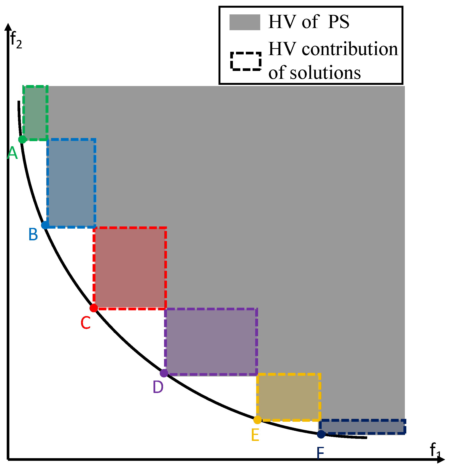
2.3. Hypervolume Contribution

In order to solve the problem of using Pareto non-dominated solutions to update the output solution set, this paper uses a comprehensive index to update the output archive. Hypervolume is a widely used performance metric that simultaneously measures both the diversity and convergence of the population. However, the computation process of HV is time-consuming and difficult due to it needing to compute the volume of the hypercube composed between the solution set and the reference point set. To reduce the computational burden of hypervolume, the HV contribution method was proposed [42]. The main idea is to calculate the HV proportion provided by a certain solution in the Pareto set. By calculating the HV contribution of each offspring solution to the current Pareto set, a new population that maximizes the hypervolume under a fixed number of solutions can be quickly identified. The concepts of HV and HV contributions are illustrated in Figure 2.

In two objective optimization problems, the algorithm implements a dual-sorting strategy: primary ascending ordering by f₁ values followed by secondary descending ordering based on f₂ values. For the sorted frontier Rv = {s₁, …, s_|Rv|}, the hypervolume contribution can be computed using Equation (2) (applicable for i = 2, …, |R_v| − 1):

HVMeasure(s,R_v) = (f₁(s_i+1) − f₁(s_i))·(f₂(s_i−1) − f₂(s_i))

(2)

3. Proposed Algorithm

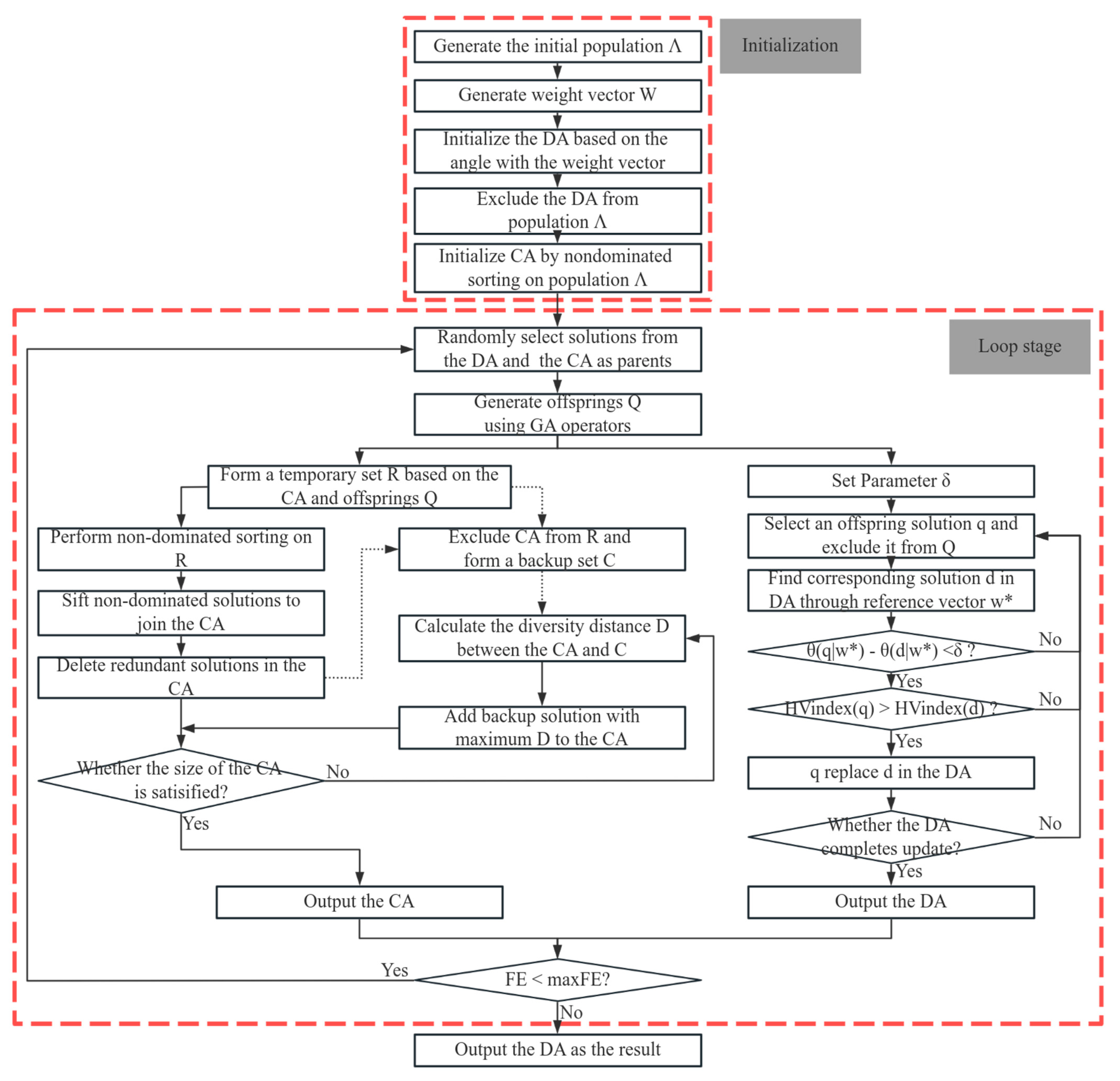
3.1. Basic Flow of TwoArchRH

The general flowchart of the proposed TwoArchRH is shown in Figure 3. The structure of TwoArchRH is similar to that of TwoArch2, but the main components are totally different. The pseudocode of the proposed method is shown in Algorithm 1. The algorithm initializes and updates the convergence archive and diversity archive by various metrics such as weight vector and hypervolume contribution and outputs the diversity archive at the end of the algorithm.

Algorithm 1: TwoArchRH Framework
Input: N(Population size), maxFE
Output: DA
//Initialization
1:	Λ ← RamdomInitialize(3N)
2:	W ← UniformWeightVectors(N)
3:	B = pdist2(W,W);
4:	[~,B] = sort(B,2);
5:	nearby = B(:,1:(N/10));
6:	$\mathrm{DA} \leftarrow \left\{\underset{\mathrm{j}\in \left\{1,\cdots ,\mathrm{N}\right\}}{\arg \min }\mathsf{\theta }({\mathbf{f}}_{\mathrm{i}}|{\mathbf{w}}_{\mathrm{j}})\right\}$
7:	Λ = Λ\DA
8:	CA ← FastNondominatedSort(Λ)
//Ioop stage
9:	while FE < maxFE do
10:	Q ← GenerateOffspring(CA, DA)
11:	DA ← UpdateDA(DA,Q,W)
12:	CA ← UpdateCA(CA,Q,W)
13:	end while

The main framework of TwoArchRH consists of initialization and loop components. In the initialization stage, a population Λ containing 3N individuals, randomly generated within the decision space, is initialized. Next, a set of N uniformly distributed reference vectors is predefined according to the method mentioned in [43]. The neighborhood relationship between vectors is recorded into a list for subsequent use. The angles between each reference vector and each initial individual solution are calculated according to Equation (3).

$$\mathsf{\theta }({\mathbf{f}}_{\mathrm{i}}|{\mathbf{w}}_{\mathrm{j}})=\arccos \left({\displaystyle \frac{{\mathbf{f}}_{\mathrm{i}}·{\mathbf{w}}_{\mathrm{j}}}{\left|{\mathbf{f}}_{\mathrm{i}}\right|\left|{\mathbf{w}}_{\mathrm{j}}\right|}}\right)$$

(3)

$${\mathrm{X}}_{\mathrm{i}|\mathrm{k}}=\underset{\mathrm{j}\in \left\{1,\cdots ,\mathrm{N}\right\}}{\arg \min }\mathsf{\theta }({\mathbf{f}}_{\mathrm{i}}|{\mathbf{w}}_{\mathrm{j}})$$

(4)

$${\mathrm{DA}}_{\mathrm{initial}}=\left\{{\mathrm{X}}_{\mathrm{i}|\mathrm{k}}\right\},\left(\mathrm{k}=1,\cdots ,\mathrm{N}\right)$$

(5)

Since the update of the diversity archive is judged by the contribution of the solution in the neighborhood population, it is necessary to ensure that any solution can find the corresponding neighborhood population through the associated reference vector. Therefore, the size of the diversity archive is the same as the number of reference vectors, and then the diversity archive is initialized by associating a solution for each reference vector. Then, the solution in the initial diversity archive is excluded from the initial population, and the size of the convergence archive is set to be the same as that of the diversity archive so that one solution is selected from each of the two archives as the parent generation. The generation of the offspring population is shown in Algorithm 2. The initialization and update methods of the convergence archive are the same. The non-dominated solutions in the initial population are screened by the reference vector, and then the diversity-intensive solutions are added to the remaining part of the archive to maintain the balance.

Algorithm 2: GenerateOffspring(CA, DA)
Input: CA, DA
Output: Q
1:	randCA ← randperm(CA)
2:	randDA ← randperm(DA)
3:	for i++<N do
4:	Q(i) = OperatorGAhalf(randCA(i),randDA(i))
5:	end for

In the next two sections, the two main components of the proposed TwoArchRH, namely DA updating and CA updating, are illustrated in detail.

3.2. Convergence Archive Updating

In MOEAs, convergence plays an important role in enforcing the population approach to the PF, especially when with objective surging. As the number of objectives surges, the search space of the MOPs also expands significantly. However, due to the restricted population size, it is challenging for a population to fully cover the Pareto front in such an expansive search space. In such cases, the population tends to represent parts of the true PF. Performing convergence-based selection on such a population tends to result in individuals with similar characteristics. Consequently, the evolutionary pressure exerted by these similar individuals becomes uniform in later stages, which can deteriorate the convergence performance of archive-based MOEAs. To enhance convergence performance, measures are adopted during the updating phase of the CA in the proposed TwoArchRH to prevent premature stagnation. Algorithm 3 illustrates the CA updating process in TwoArchRH. After the offsprings are generated, a temporary population R, which consists of the offsprings and the individuals of the CA, is established, and then all the non-dominated solutions in R are obtained. To provide sufficient and effective convergence pressure, a vector-based prescreen strategy is utilized in the CA. The strategy uses the existing reference vectors as the basis and calculates the angles between the non-dominated solutions in R and reference vectors to slightly introduce diversity characteristics. The reference vector is used to divide the target space so that at most one non-dominated solution is retained in each space, and introducing the opposite characteristic solutions can improve the diversity of the population. These measures help to solve the problem that the proportion of non-dominated solutions rises rapidly as the number of objectives increases, which affects the effect of the ManyOPs. The angle is calculated according to Equation (3). Based on the angle value, all the non-dominated solutions are bounded to a certain vector. Each vector then selects the unique non-dominated solution with the smallest angle, avoiding archive aggregation by the reference vector filtering strategy. The selected non-dominated solutions are stored in a temporary set Ω. If the size of Ω is smaller than that of the CA, some solutions are selected from the currently unselected solutions to complete the archive, and these selected ones form a new CA together with the solutions in Ω. The selection process is illustrated as Lines 6 to 13 in Algorithm 3 and is based on diversity distance which can be calculated as in Equation (6).

$${\mathrm{d}}_{\min }(\mathrm{r},\mathrm{CA})=\min \left\{\sqrt{{\left({\mathrm{r}}_1-{\mathrm{q}}_{\mathrm{i}1}\right)}^2+...+{\left({\mathrm{r}}_{\mathrm{n}}-{\mathrm{q}}_{\mathrm{in}}\right)}^2}\right\}$$

(6)

where r = (r₁, r₂…, r_n) represents the coordinates of the candidate solution and Q_i = (q_i1, q_i2, …, q_in) represents the coordinates of the solution in Ω.

Algorithm 3: UpdateCA(CA,Q,W)
Input: Q(Offsprings), CA, W(reference vectors)
Output: CA
1:	R = CA ∪ Q
2:	R1 ← non-dominated sort R
3:	$\forall {\mathrm{R}1}_{\mathrm{i}}\in \mathrm{R}1,{\mathrm{W}}^{\prime }=\underset{\mathrm{w}\in \mathrm{W}}{\mathrm{argmin}}\left(\mathsf{\theta }({\mathrm{R}1}_{\mathrm{i}}|{\mathbf{w}}_{\mathrm{j}})\right)$
4:	W’ = unique(W’)
5:	$\forall {\mathrm{w}}_{\mathrm{i}} \in {\mathrm{W}}^{\prime }, \mathsf{\Omega }=\left\{\underset{\mathrm{c}\in \mathrm{CA}}{\mathrm{argmin}}\left(\arccos \left({\displaystyle \frac{{\mathrm{w}}_{\mathrm{i}}\cdot \mathrm{c}}{\parallel {\mathrm{w}}_{\mathrm{i}}\parallel \parallel \mathrm{c}\parallel }}\right)\right)\right\}$
6:	if size(Ω) < size(CA) then
7:	C = R\Ω
8:	for i = 1: size(C) do
9:	$\mathrm{D}\left(\mathrm{i}\right){\leftarrow \mathrm{d}}_{\min }\left(\mathrm{C}\right(\mathrm{i}),\mathsf{\Omega })=\min \left\{\sqrt{{\left({\mathrm{c}}_1-{\mathrm{t}}_{\mathrm{i}1}\right)}^2+{\left({\mathrm{c}}_2-{\mathrm{t}}_{\mathrm{i}2}\right)}^2+\dots +{\left({\mathrm{c}}_{\mathrm{n}}-{\mathrm{t}}_{\mathrm{in}}\right)}^2}\right\}$
10:	end for
11:	maxI = find(D == max(D))
12:	Ω = Ω ∪ C(maxI)
13:	end if
14:	CA = Ω

3.3. Diversity Archive Updating

The diversity property of population plays an important role in maintaining a well-distributed pareto set. In ManyOPs, the surge in objectives means that most individuals are non-dominated. Traditional diversity-only metrics are inclined to sift solutions with extreme objective values. For example, the dominance-resistant solutions have a small value on one objective, while the values on the other objectives are large. In that case, the extreme solutions make the population diverge in space and undermine the evolving pressure. Thus, traditional diversity-only metrics do not effectively provide sufficient selection criterion.

Indicators like the HV and IGD provide overall performance comparisons and can complement individual selection, but they are computationally intensive. The HV contributor mentioned in Section 2 offers a practical alternative to HV. It measures the hypervolume component of each solution within its nearby domain and then calculates a component ratio to represent the importance of the solution. The nearby domain of a solution is determined by the neighboring solutions which are screened by the sorting method proposed by SMS-EMOA. However, for more than two objectives, the sorting sequence becomes impractical due to the multiple comparisons required, posing a significant drawback for the HV contributor. On the basis of the above discussion, the HVindex inspired by the HV contributor is proposed in this work to ameliorate the HV calculation and assist the updating of the DA. The pseudocode of the HVindex is shown in Algorithm 4.

Algorithm 4: HVIndex(q,W,DA)
Input: Q(Offsprings), DA, W(reference vectors)
Output: DA
1:	${\mathrm{w}}^{*}=\underset{{\mathrm{w}}_{\mathrm{i}}\in \mathrm{W}}{\min }\mathsf{\theta }(\mathrm{q}{|\mathrm{w}}_{\mathrm{i}})$
2:	W’ = nearby(w*)
3:	D = DA(w*)
4:	D = DA(W’)
5:	if$\mathsf{\theta }(\mathrm{q}|\mathrm{w}*)$ − $\mathsf{\theta }(\mathrm{d}|\mathrm{w}*)$< δ then
6:	c1 ← HVContri(q,D∪q)
7:	c2 ← HVContri(d,D∪d)
8:	if c1 > c2
9:	DA(w*) = q
10:	end if
11:	end if

The proposed HVindex includes nearby domain determination and substitute solution comparison. The nearby domain of a solution is determined by neighboring solutions which are obtained in the reference vector framework. Firstly, each offspring individual is attached to a certain reference vector according to the angle calculated by Equation (3).

Once the reference vector is determined, nearby vectors can be identified by searching the vector list. Since each reference vector corresponds to a solution in the DA, the nearby solutions and the nearby domain can be quickly retrieved. Within the nearby domain, the ratio-based HV contributor can be calculated as in Equation (7).

$$\mathrm{HVContri}\left(\mathrm{x},\mathsf{\Omega }\right)=\prod _{\mathrm{i}=1}^{\mathrm{M}}\underset{\mathrm{X}\in \mathsf{\Omega }}{\min }\left|{\mathrm{f}}_{\mathrm{i}}\left(\mathrm{x}\right) - {\mathrm{f}}_{\mathrm{i}}\left(\mathrm{X}\right)\right|$$

(7)

where x is the solution, is the set that comprises nearby solutions, and denotes the ith-objective value, while M is the sum number of objectives.

Since both the substitute solution and the original solution are assigned to the same reference vector, their nearby domain Ω is identical. Additionally, a comparison control parameter δ is introduced to further reduce the computational needs. Since the goal of the DA is to maintain a subpopulation that ensures sufficient diversity, the replacement of individuals in the DA must prioritize uniform distribution. Parameter δ is an angle threshold that tolerates the maximum deviation to the reference vector more than the corresponding DA solution. If the offspring x is further away from the reference vector w* than DA(w*), it is neglected due to how it undermines the even distribution of the DA. The angular comparison within the reference vector-based framework can be used to effectively measure diversity and uses the threshold δ to increase the comparison range, which can reserve more potential solutions for further comparisons. Next, a further comparison is conducted based on HVContri. If the substitute solution has a better HVContri than that of DA(w*), the substitute solution is replaced to form the new DA. The pseudocode for updating the DA is shown in Algorithm 5.

Algorithm 5: UpdateDA(CA,Q,W)
Input: Q(Offsprings), DA, W(reference vectors)
Output: DA
1:	for j = 1: size(Q)
2:	HVindex(Q(j),W,DA)
3:	end for

4. Parametric Study of TwoArchRH

In this section, the parametric study includes the effect of opposite characteristic solutions and the effect of threshold δ. All the algorithm source codes and test problems in this paper are obtained on a platform called PlatEMO (Matlab version: R2023b 64-bit) [44]. In order to ensure the fairness of the experiment, all the experiments were carried out on this platform.

Since DTLZ1 is a representative difficult convergence problem, if TwoArchRH is tuned to the best state on DTLZ1, a similar performance can be observed on other issues. Therefore, DTLZ1 is used as a test example to tune TwoArchRH.

4.1. Effect of Opposite Characteristic Solutions

A significant feature of TwoArchRH is that the archive contains opposite characteristic solutions to avoid the premature convergence of the population. To assess the impact of this enhancement, we modified the CA updating process in TwoArchRH while keeping the other components unchanged, resulting in a comparison algorithm. In the comparison algorithm, the convergence archive uses non-dominated sorting to select the non-dominated solution and then filters the non-dominated solution through the reference vector. Finally, the archive is completed by calculating the distance between the candidate solution and the ideal point.

Table 1. Effect of opposite characteristic solutions.

Metric	M	TwoArchRH	Comparison Algorithm
HV	5	9.8000 × 10−1 (1.36 × 10−4)	9.7879 × 10−1 (1.27 × 10−5)
	8	9.9750 × 10−1 (1.92 × 10−4)	9.9684 × 10−1 (1.42 × 10−4)
	10	9.9964 × 10−1 (2.62 × 10−5)	9.9842 × 10−1 (1.47 × 10−4)

shows the HV metrics of these two algorithms on DTLZ1, revealing that including solutions with opposite characteristics in the CA improves the algorithm’s performance.

4.2. Effect of Threshold δ

The value of δ is crucial in the updating process of the DA; an excessively high or low δ can negatively impact the overall performance of the algorithm. A large δ affects the prescreening ability and prolongates the updating time while a small δ leads to strict screening and deteriorates the performance. We tested the DTLZ1 and compared the most suitable parameter δ value in three cases where the number of objectives was equal to 5, 8 and 10. The results of the HV and running time are shown in

Table 2. Effect of threshold δ.

	Hypervolume			Runtime
	M = 5	M = 8	M = 10	M = 5	M = 8	M = 10
δ = 1	9.7871 × 10−1 (2.26 × 10−4)	9.6722 × 10−1 (2.13 × 10−2)	9.7742 × 10−1 (4.73 × 10−2)	1.5221 × 103 (2.42 × 101)	1.4398 × 103 (7.38 × 101)	4.4237 × 103 (4.36 × 101)
δ = 2	9.7940 × 10−1 (3.06 × 10−4)	9.9659 × 10−1 (6.37 × 10−4)	9.9285 × 10−1 (3.24 × 10−2)	1.9053 × 103 (3.07 × 101)	1.8082 × 103 (2.40 × 101)	4.8125 × 103 (2.45 × 101)
δ = 3	9.7962 × 10−1 (1.05 × 10−4)	9.9746 × 10−1 (1.62 × 10−4)	9.9946 × 10−1 (1.53 × 10−4)	2.1550 × 103 (4.33 × 101)	2.0454 × 103 (1.07 × 101)	5.0454 × 103 (2.16 × 101)
δ = 4	9.7966 × 10−1 (5.35 × 10−4)	9.9741 × 10−1 (1.75 × 10−4)	9.9941 × 10−1 (1.86 × 10−4)	2.3219 × 103 (4.48 × 101)	2.3168 × 103 (2.46 × 101)	5.3362 × 103 (2.53 × 101)
δ = 5	9.8000 × 10−1 (1.36 × 10−4)	9.9750 × 10−1 (1.92 × 10−4)	9.9964 × 10−1 (2.62 × 10−5)	2.4766 × 103 (1.18 × 101)	2.4191 × 103 (2.91 × 101)	5.4527 × 103 (2.91 × 101)
δ = 6	9.7947 × 10−1 (2.25 × 10−4)	9.9751 × 10−1 (1.84 × 10−4)	9.9962 × 10−1 (1.65 × 10−4)	2.6042 × 103 (3.41 × 100)	2.5635 × 103 (2.53 × 101)	5.5435 × 103 (2.66 × 101)
δ = 7	9.7952 × 10−1 (3.54 × 10−4)	9.9754 × 10−1 (9.76 × 10−4)	9.9970 × 10−1 (8.65 × 10−5)	2.7114 × 103 (4.09 × 101)	2.6846 × 103 (1.23 × 101)	5.6237 × 103 (1.89 × 101)
δ = 8	9.7933 × 10−1 (2.96 × 10−4)	9.9750 × 10−1 (1.80 × 10−4)	9.9979 × 10−1 (1.44 × 10−4)	2.7313 × 103 (4.24 × 101)	2.7658 × 103 (4.74 × 100)	5.7358 × 103 (4.56 × 101)
δ = 9	9.7940 × 10−1 (1.62 × 10−4)	9.9746 × 10−1 (6.93 × 10−4)	9.9973 × 10−1 (7.74 × 10−5)	2.7996 × 103 (1.37 × 101)	2.7942 × 103 (3.17 × 101)	5.7942 × 103 (2.76 × 101)
δ = 10	9.7941 × 10−1 (1.63 × 10−5)	9.9740 × 10−1 (1.84 × 10−5)	9.9969 × 10−1 (2.35 × 10−5)	2.8546 × 103 (3.56 × 100)	2.9521 × 103 (1.07 × 102)	5.9251 × 103 (1.14 × 102)
δ = 11	9.7942 × 10−1 (2.15 × 10−4)	9.9743 × 10−1 (2.56 × 10−4)	9.9962 × 10−1 (2.39 × 10−5)	2.8563 × 103 (6.87 × 100)	2.9785 × 103 (3.52 × 101)	6.0835 × 103 (2.76 × 101)
δ = 12	9.7920 × 10−1 (2.33 × 10−5)	9.9721 × 10−1 (1.66 × 10−4)	9.9954 × 10−1 (1.75 × 10−4)	2.8938 × 103 (6.27 × 101)	2.9583 × 103 (1.93 × 101)	6.1253 × 103 (1.67 × 101)
δ = 13	9.7928 × 10−1 (4.30 × 10−4)	9.9735 × 10−1 (8.70 × 10−5)	9.9952 × 10−1 (7.67 × 10−5)	2.8686 × 103 (9.82 × 100)	3.0667 × 103 (3.58 × 101)	6.2687 × 103 (2.45 × 101)
δ = 14	9.7896 × 10−1 (2.61 × 10−4)	9.9727 × 10−1 (3.18 × 10−5)	9.9942 × 10−1 (3.24 × 10−5)	2.9450 × 103 (3.86 × 101)	3.0995 × 103 (2.47 × 101)	6.3895 × 103 (2.43 × 101)
δ = 15	9.7890 × 10−1 (6.69 × 10−4)	9.9720 × 10−1 (1.28 × 10−4)	9.9948 × 10−1 (1.35 × 10−4)	2.9372 × 103 (6.07 × 101)	3.1142 × 103 (2.13 × 101)	6.4246 × 103 (2.63 × 101)

.

The table shows that as δ decreases, the algorithm’s running time shortens. However, with an increasing number of objectives, δ should be set larger. Despite this, the table indicates that the running time increases with δ. Considering both the HV and runtime, δ = 5 is found to be optimal for the proposed TwoArchRH.

5. Experiments and Results

To analyze the behavior of TwoArchRH, we compare TwoArchRH with TwoArch2, PeEA [15], and VaEA [11] on 27 MOPs with different numbers of objectives. These are many-objective optimization algorithms based on improved two archives. Based on the improved dominance relations and based on the reference vector, these algorithms are among the better optimization algorithms of the class. The test problems include ZDT1-3 [45], BT1-9 [46], WFG1-9 [47], and DTLZ1-6 [48]; the number of objectives and other parameter settings for the test problems are listed in

Table 3. Parameter setting for test problems.

Test Set	Objective	Population Size	Decision Variables
ZDT	M = 2	N = 100	D = 30
BT	M = 2	N = 100	D = 30
DTLZ1	M = 5, 8, 10	N = 210, 156, 275	D = M − 1 + 5
DTLZ{2–6}	M = 5, 8, 10	N = 210, 156, 275	D = M − 1 + 10
WFG{1, 2, 4–9}	M = 5, 8, 10	N = 210, 156, 275	D = M − 1 + 10
WFG3	M = 5, 8, 10	N = 210, 156, 275	D = M − 1 + 6

. Each algorithm is independently run 30 times on each test instance. The maximum number of FEs is set to 300,000 as the termination criterion. To assess the performance, the HV [49] and IGD [50] are selected as the performance metric. The larger the HV value, the better the quality of the obtained solutions to approximate the whole PF. The HV is approximated by the Monte Carlo simulation [51] to reduce the computational complexity. The mean and standard deviations are noted, with the best mean for each problem highlighted in bold.

5.1. Experiments on Two-Objective Problems

Table 4. The HV values (mean and standard deviation) obtained by TwoArchRH, TwoArch2, PeEA, and VaEA on the ZDT and BT test suite.

Problem	N	M	D	TwoArchRH	TwoArch2	PeEA	VaEA
ZDT1	100	2	30	7.2013 × 10−1 (6.44 × 10−5)	7.2035 × 10−1 (7.19 × 10−8)	7.1884 × 10−1 (8.78 × 10−5)	7.1886 × 10−1 (2.86 × 10−4)
ZDT2	100	2	30	4.4503 × 10−1 (2.00 × 10−5)	4.4496 × 10−1 (1.95 × 10−8)	4.4457 × 10−1 (3.04 × 10−4)	4.4347 × 10−1 (2.84 × 10−4)
ZDT3	100	2	30	7.3649 × 10−1 (4.86 × 10−2)	5.9961 × 10−1 (7.54 × 10−5)	5.9940 × 10−1 (2.78 × 10−4)	5.9642 × 10−1 (5.10 × 10−4)
BT1	100	2	30	7.1636 × 10−1 (5.61 × 10−4)	6.8414 × 10−1 (3.09 × 10−5)	7.0633 × 10−1 (5.72 × 10−3)	7.1622 × 10−1 (6.90 × 10−4)
BT2	100	2	30	5.8740 × 10−1 (1.25 × 10−2)	5.2916 × 10−1 (9.04 × 10−3)	5.7222 × 10−1 (2.71 × 10−2)	6.6839 × 10−1 (2.83 × 10−3)
BT3	100	2	30	7.1595 × 10−1 (1.09 × 10−3)	7.0907 × 10−1 (7.95 × 10−3)	7.0221 × 10−1 (5.84 × 10−2)	7.0793 × 10−1 (1.60 × 10−3)
BT4	100	2	30	7.1681 × 10−1 (4.51 × 10−4)	7.0933 × 10−1 (1.22 × 10−3)	7.0647 × 10−1 (2.85 × 10−4)	7.1364 × 10−1 (9.44 × 10−4)
BT5	100	2	30	6.6169 × 10−1 (1.11 × 10−4)	5.7766 × 10−1 (9.67 × 10−2)	6.5142 × 10−1 (2.37 × 10−3)	6.5816 × 10−1 (2.98 × 10−4)
BT6	100	2	30	5.0736 × 10−1 (1.75 × 10−3)	3.8959 × 10−1 (1.04 × 10−2)	3.7553 × 10−1 (1.49 × 10−2)	3.6821 × 10−1 (6.00 × 10−2)
BT7	100	2	30	5.9285 × 10−1 (1.71 × 10−3)	4.6545 × 10−1 (1.00 × 10−4)	5.4039 × 10−1 (1.22 × 10−3)	5.2923 × 10−1 (4.80 × 10−4)
BT8	100	2	30	4.0481 × 10−1 (2.02 × 10−3)	3.3353 × 10−1 (5.05 × 10−3)	3.8509 × 10−1 (2.73 × 10−3)	3.7903 × 10−1 (5.66 × 10−2)

and

Table 5. The IGD values (mean and standard deviation) obtained by TwoArchRH, TwoArch2, PeEA, and VaEA on the ZDT and BT test suite.

Problem	N	M	D	TwoArchRH	TwoArch2	PeEA	VaEA
ZDT1	100	2	30	3.8473 × 10−3 (1.44 × 10−3)	3.7664 × 10−3 (4.80 × 10−2)	5.1405 × 10−3 (1.30 × 10−2)	4.7815 × 10−3 (3.74 × 10−3)
ZDT2	100	2	30	3.8419 × 10−3 (4.50 × 10−3)	4.7693 × 10−3 (4.57 × 10−2)	5.2376 × 10−3 (3.49 × 10−2)	4.2596 × 10−3 (1.92 × 10−3)
ZDT3	100	2	30	8.7326 × 10−2 (1.09 × 10−2)	4.4386 × 10−3 (1.72 × 10−3)	1.3076 × 10−2 (4.99 × 10−3)	5.7783 × 10−3 (7.45 × 10−2)
BT1	100	2	30	5.2708 × 10−2 (1.39 × 10−2)	2.8902 × 10−2 (2.47 × 10−2)	6.2546 × 10−3 (4.86 × 10−3)	1.0560 × 10−2 (4.43 × 10−3)
BT2	100	2	30	1.0261 × 10−1 (9.43 × 10−3)	1.5330 × 10−1 (8.33 × 10−3)	3.9400 × 10−2 (2.13 × 10−3	1.1424 × 10−1 (2.80 × 10−2)
BT3	100	2	30	5.3496 × 10−3 (5.04 × 10−3)	9.5283 × 10−3 (5.22 × 10−3)	1.0274 × 10−2 (1.47 × 10−3)	1.1237 × 10−2 (1.73 × 10−3)
BT4	100	2	30	6.0098 × 10−3 (6.20 × 10−3)	9.8765 × 10−3 (9.92 × 10−2)	1.0886 × 10−2 (1.01 × 10−3)	1.2979 × 10−2 (5.74 × 10−3)
BT5	100	2	30	4.1277 × 10−3 (1.19 × 10−2)	6.8158 × 10−2 (7.95 × 10−2)	6.9714 × 10−3 (9.23 × 10−3)	8.1935 × 10−3 (1.13 × 10−3)
BT6	100	2	30	1.6133 × 10−1 (7.13 × 10−2)	3.2087 × 10−1 (2.00 × 10−3)	3.2319 × 10−1 (1.21 × 10−2)	2.6637 × 10−1 (3.72 × 10−2)
BT7	100	2	30	8.7662 × 10−2 (1.45 × 10−3)	3.0271 × 10−1 (2.35 × 10−1)	2.4751 × 10−1 (8.26 × 10−2)	1.5947 × 10−1 (7.93 × 10−3)
BT8	100	2	30	2.8210 × 10−1 (5.18 × 10−2)	3.4574 × 10−1 (3.42 × 10−3)	2.5042 × 10−1 (1.59 × 10−2)	3.0723 × 10−1 (1.86 × 10−2)

show the HV and IGD values for TwoArchRH, TwoArch2, PeEA, and VaEA on the ZDT and BT test suites, with the best results highlighted. According to Table 4, TwoArchRH excels in 9 out of 11 HV tests, notably on ZDT3, where it outperforms others. On BT problems, TwoArchRH leads except on BT2, where VaEA achieves the best HV. Table 5 indicates TwoArchRH excels in 8 out of 11 IGD tests, particularly on BT1–BT8 except BT2, where PeEA performs best.

From the experimental results, it can be seen that TwoArchRH has a significant improvement on the ZDT3 and BT6-8 test problems compared to the other algorithms; ZDT3 has a discontinuous Pareto front, which presents an additional challenge to identify all the unconnected regions. TwoArchRH achieves the most significant improvement on ZDT3 compared to the other benchmark algorithms, which can be attributed to its strategy of evaluating the overall enhancement in the neighborhood population through hypervolume contribution, effectively addressing discontinuity issues through overall evaluation. BT6 and BT8 possess a simple nonlinear PS, but BT7 features a complex nonlinear PS. The excellent performance of TwoArchRH on these three test problems proves that the balance strategy of TwoArchRH can adapt to the complex search space. On BT2, however, TwoArchRH did not achieve better results, probably because BT2 is a distance-dependent bias problem, and TwoArchRH’s strategy of relying on Euclidean distance to assess diversity is difficult to deal with.

5.2. Experiments on the DTLZ Problems

Table 6. The HV values (mean and standard deviation) obtained by TwoArchRH, TwoArch2, PeEA, and VaEA on the DTLZ test suite.

Problem	N	M	D	TwoArchRH	TwoArch2	PeEA	VaEA
DTLZ1	210	5	10	9.8000 × 10−1 (1.36 × 10−4)	9.7543 × 10−1 (7.50 × 10−4)	9.6577 × 10−1 (1.44 × 10−3)	8.8046 × 10−1 (1.77 × 10−2)
	156	8	12	9.9750 × 10−1 (1.92 × 10−4)	9.8958 × 10−1 (2.04 × 10−4)	9.9555 × 10−1 (4.95 × 10−3)	8.8706 × 10−1 (7.73 × 10−3)
	275	10	14	9.9964 × 10−1 (2.62 × 10−5)	9.9565 × 10−1 (7.07 × 10−5)	9.9955 × 10−1 (7.57 × 10−5)	9.6961 × 10−1 (1.19 × 10−2)
DTLZ2	210	5	14	8.1020 × 10−1 (4.98 × 10−4)	7.6529 × 10−1 (3.49 × 10−3)	8.0116 × 10−1 (1.02 × 10−3)	7.8968 × 10−1 (2.48 × 10−3)
	156	8	17	9.3352 × 10−1 (4.05 × 10−4)	8.1060 × 10−1 (1.47 × 10−2)	8.9457 × 10−1 (1.21 × 10−3)	9.1071 × 10−1 (2.35 × 10−4)
	275	10	19	9.7508 × 10−1 (4.40 × 10−4)	8.0053 × 10−1 (6.20 × 10−3)	9.5161 × 10−1 (1.66 × 10−2)	9.4839 × 10−1 (3.55 × 10−3)
DTLZ3	210	5	14	8.1183 × 10−1 (5.09 × 10−4)	7.9084 × 10−1 (4.14 × 10−4)	7.9567 × 10−1 (3.04 × 10−3)	4.5988 × 10−1 (4.31 × 10−1)
	156	8	17	9.3440 × 10−1 (2.33 × 10−3)	8.3173 × 10−1 (4.07 × 10−3)	8.9265 × 10−1 (1.62 × 10−3)	8.0746 × 10−1 (3.02 × 10−2)
	275	10	19	9.7514 × 10−1 (3.36 × 10−4)	8.6687 × 10−1 (2.25 × 10−3)	9.3928 × 10−1 (1.38 × 10−3)	8.0586 × 10−1 (5.70 × 10−1)
DTLZ4	210	5	14	8.1255 × 10−1 (2.40 × 10−4)	7.6273 × 10−1 (3.03 × 10−3)	7.9892 × 10−1 (1.12 × 10−4)	7.9192 × 10−1 (8.43 × 10−4)
	156	8	17	9.3333 × 10−1 (6.86 × 10−5)	7.4288 × 10−1 (3.41 × 10−3)	9.0295 × 10−1 (2.92 × 10−3)	9.0259 × 10−1 (2.31 × 10−3)
	275	10	19	9.7500 × 10−1 (3.92 × 10−4)	8.0672 × 10−1 (1.35 × 10−2)	9.5030 × 10−1 (8.15 × 10−4)	9.3955 × 10−1 (8.07 × 10−3)
DTLZ5	210	5	14	1.1340 × 10−1 (8.80 × 10−3)	1.1718 × 10−1 (6.93 × 10−4)	1.0899 × 10−1 (8.21 × 10−3)	1.0353 × 10−1 (9.45 × 10−4)
	156	8	17	9.4164 × 10−2 (1.84 × 10−3)	9.1022 × 10−2 (2.21 × 10−5)	9.6380 × 10−2 (1.45 × 10−3)	9.0976 × 10−2 (6.54 × 10−3)
	275	10	19	8.6816 × 10−1 (2.64 × 10−3)	9.1429 × 10−2 (1.36 × 10−3)	9.2084 × 10−2 (2.41 × 10−4)	9.0900 × 10−2 (5.43 × 10−6)
DTLZ6	210	5	14	1.1631 × 10−1 (2.43 × 10−3)	1.1136 × 10−1 (2.85 × 10−3)	1.1033 × 10−1 (2.46 × 10−3)	9.0561 × 10−2 (9.28 × 10−3)
	156	8	17	9.5496 × 10−2 (8.35 × 10−6)	9.0909 × 10−2 (2.41 × 10−3)	9.5076 × 10−2 (1.19 × 10−3)	9.0874 × 10−2 (1.05 × 10−4)
	275	10	19	9.0607 × 10−2 (1.27 × 10−3)	9.0909 × 10−2 (4.21 × 10−3)	9.1617 × 10−2 (8.95 × 10−4)	9.0324 × 10−2 (3.24 × 10−4)

and

Table 7. The IGD values (mean and standard deviation) obtained by TwoArchRH, TwoArch2, PeEA, and VaEA on the DTLZ test suite.

Problem	N	M	D	TwoArchRH	TwoArch2	PeEA	VaEA
DTLZ1	210	5	10	5.2395 × 10−2 (4.21 × 10−3)	5.2234 × 10−2 (1.46 × 10−2)	5.6398 × 10−2 (3.04 × 10−4)	1.1652 × 10−1 (1.46 × 10−2)
	156	8	12	9.5862 × 10−2 (2.18 × 10−1)	9.9952 × 10−2 (8.23 × 10−4)	1.0555 × 10−1 (3.07 × 10−3)	2.1739 × 10−1 (1.09 × 10−1)
	275	10	14	1.0649 × 10−1 (1.08 × 10−1)	1.0316 × 10−1 (1.42 × 10−3)	1.1394 × 10−1 (1.02 × 10−3)	1.9682 × 10−1 (1.94 × 10−2)
DTLZ2	210	5	14	1.6678 × 10−1 (9.08 × 10−3)	1.7063 × 10−1 (4.32 × 10−3)	1.7217 × 10−1 (3.01 × 10−4)	1.7000 × 10−1 (3.72 × 10−3)
	156	8	17	3.4743 × 10−1 (8.29 × 10−2)	3.7971 × 10−1 (5.50 × 10−3)	3.6911 × 10−1 (4.75 × 10−3)	3.6517 × 10−1 (1.33 × 10−3)
	275	10	19	4.4915 × 10−1 (6.76 × 10−5)	4.1208 × 10−1 (5.48 × 10−4)	3.9612 × 10−1 (9.52 × 10−4)	4.1140 × 10−1 (4.25 × 10−3)
DTLZ3	210	5	14	1.6609 × 10−1 (3.35 × 10−5)	1.6645 × 10−1 (2.10 × 10−3)	1.7852 × 10−1 (4.28 × 10−3)	4.9062 × 10−1 (8.37 × 10−1)
	156	8	17	3.4959 × 10−1 (5.88 × 10−3)	3.6719 × 10−1 (1.33 × 10−3)	3.7259 × 10−1 (5.29 × 10−3)	4.5920 × 10−1 (1.61 × 100)
	275	10	19	4.5142 × 10−1 (4.20 × 10−3)	4.0761 × 10−1 (4.01 × 10−3)	4.0153 × 10−1 (2.97 × 10−3)	5.6151 × 10−1 (1.64 × 10−3)
DTLZ4	210	5	14	1.6694 × 10−1 (7.62 × 10−4)	1.7223 × 10−1 (6.66 × 10−4)	1.7140 × 10−1 (1.04 × 10−3)	1.6911 × 10−1 (1.26 × 10−3)
	156	8	17	3.4819 × 10−1 (2.44 × 10−5)	3.8412 × 10−1 (3.59 × 10−3)	3.6552 × 10−1 (1.75 × 10−3)	3.6373 × 10−1 (1.79 × 10−4)
	275	10	19	4.5091 × 10−1 (1.05 × 10−3)	4.1177 × 10−1 (1.33 × 10−3)	3.9965 × 10−1 (1.36 × 10−3)	4.2174 × 10−1 (5.95 × 10−3)
DTLZ5	210	5	14	6.7981 × 10−2 (1.16 × 10−2)	6.1715 × 10−2 (1.20 × 10−2)	5.8573 × 10−2 (3.49 × 10−2)	1.0739 × 10−1 (1.81 × 10−2)
	156	8	17	1.6240 × 10−1 (6.22 × 10−2)	2.1816 × 10−1 (2.55 × 10−2)	7.4070 × 10−2 (2.33 × 10−2)	3.2391 × 10−1 (1.02 × 10−1)
	275	10	19	1.9185 × 10−1 (5.36 × 10−2)	1.7578 × 10−1 (1.93 × 10−2)	3.7576 × 10−2 (1.15 × 10−2)	5.1925 × 10−1 (2.27 × 10−1)
DTLZ6	210	5	14	8.0945 × 10−2 (2.56 × 10−2)	9.1242 × 10−2 (4.15 × 10−2)	7.2563 × 10−2 (7.68 × 10−3)	2.1490 × 10−1 (3.60 × 10−3)
	156	8	17	1.6150 × 10−1 (1.59 × 10−1)	3.9552 × 10−1 (1.16 × 10−1)	1.2853 × 10−1 (5.97 × 10−3)	3.4230 × 10−1 (5.04 × 10−1)
	275	10	19	2.5863 × 10−1 (1.65 × 10−1)	3.6338 × 10−1 (2.43 × 10−2)	7.5299 × 10−2 (3.31 × 10−2)	1.0370 × 100 (4.04 × 10−1)

present the HV and IGD values for TwoArchRH, TwoArch2, PeEA, and VaEA on the DTLZ suite, with the best results highlighted. According to Table 6, TwoArchRH excels in 14 out of 18 HV tests, especially on DTLZ1–DTLZ4 across all objectives. However, PeEA and TwoArch2 outperform it on DTLZ5 and DTLZ6 in some cases. Table 7 shows TwoArchRH leading in 11 out of 18 IGD tests, excelling on DTLZ2–DTLZ4, while PeEA dominates on DTLZ5 and DTLZ6.

From the experimental results, it can be seen that the HV value of TwoArchRH is excellent on all the DTLZ test problems except DTLZ5. The Pareto front of DTLZ5 is degenerated into a one-dimensional curve, which tests the performance of the algorithm in low-dimensional embedded high-dimensional space. The performance of TwoArchRH on the degradation problem may be due to the uniform distribution of reference vectors and the strategy of relying on reference vectors to update the population, resulting in the algorithm retaining a large number of solutions in the invalid target space. With regard to the IGD results, TwoArchRH performs poorly on high-dimensional many-objective optimization problems with M = 10, reflecting that the algorithm is slightly insufficient in diversity maintenance. This may be because it is difficult to judge the relationship between solutions when the number of targets is large through the hypervolume contribution strategy in the neighborhood population.

5.3. Experiments on the WFG Problems

Table 8. The HV values (mean and standard deviation) obtained by TwoArchRH, TwoArch2, PeEA, and VaEA on the WFG test suite.

Problem	N	M	D	TwoArchRH	TwoArch2	PeEA	VaEA
WFG1	210	5	10	9.9764 × 10−1 (2.14 × 10−5)	9.9658 × 10−1 (9.19 × 10−6)	9.9195 × 10−1 (5.57 × 10−4)	9.9798 × 10−1 (8.37 × 10−4)
	156	8	12	9.9971 × 10−1 (4.53 × 10−5)	9.9810 × 10−1 (6.72 × 10−4)	9.9644 × 10−1 (2.70 × 10−4)	9.9997 × 10−1 (1.03 × 10−4)
	275	10	14	9.9974 × 10−1 (3.50 × 10−2)	9.9906 × 10−1 (4.17 × 10−5)	9.9791 × 10−1 (1.93 × 10−1)	9.9998 × 10−1 (9.49 × 10−3)
WFG2	210	5	14	9.9612 × 10−1 (2.06 × 10−4)	9.9677 × 10−1 (9.47 × 10−5)	9.7684 × 10−1 (5.59 × 10−3)	9.9076 × 10−1 (7.47 × 10−4)
	156	8	17	9.9832 × 10−1 (1.16 × 10−3)	9.9842 × 10−1 (3.48 × 10−4)	9.8555 × 10−1 (4.45 × 10−3)	9.9721 × 10−1 (7.01 × 10−4)
	275	10	19	9.9712 × 10−1 (6.66 × 10−4)	9.9927 × 10−1 (7.01 × 10−5)	9.9072 × 10−1 (1.26 × 10−4)	9.9649 × 10−1 (1.17 × 10−3)
WFG3	210	5	14	2.0164 × 10−1 (3.25 × 10−3)	2.2571 × 10−1 (5.28 × 10−3)	1.9380 × 10−1 (2.98 × 10−2)	1.5971 × 10−1 (2.04 × 10−2)
	156	8	17	9.2170 × 10−2 (4.13 × 10−3)	8.2827 × 10−2 (7.90 × 10−3)	8.7951 × 10−1 (1.32 × 10−4)	9.0586 × 10−2 (2.13 × 10−3)
	275	10	19	0.0000 × 100 (0.00 × 100)	7.3065 × 10−2 (3.45 × 10−3)	9.1145 × 10−2 (2.42 × 10−4)	9.0186 × 10−2 (3.35 × 10−3)
WFG4	210	5	14	7.9564 × 10−1 (4.37 × 10−4)	7.6485 × 10−1 (1.58 × 10−3)	7.6376 × 10−1 (6.25 × 10−3)	7.7623 × 10−1 (8.71 × 10−4)
	156	8	17	9.0982 × 10−1 (1.13 × 10−4)	8.2826 × 10−1 (1.88 × 10−3)	8.5858 × 10−1 (6.38 × 10−4)	8.9404 × 10−1 (8.00 × 10−4)
	275	10	19	9.5606 × 10−1 (9.65 × 10−4)	8.7268 × 10−1 (8.06 × 10−4)	9.1992 × 10−1 (4.68 × 10−3)	9.3330 × 10−1 (1.66 × 10−3)
WFG5	210	5	14	7.4431 × 10−1 (7.76 × 10−4)	7.1871 × 10−1 (4.64 × 10−3)	7.2492 × 10−1 (5.88 × 10−3)	7.4196 × 10−1 (1.11 × 10−3)
	156	8	17	8.4777 × 10−1 (1.92 × 10−4)	7.7292 × 10−1 (8.45 × 10−3)	8.1280 × 10−1 (7.76 × 10−3)	8.4812 × 10−1 (2.45 × 10−3)
	275	10	19	8.9244 × 10−1 (6.57 × 10−5)	8.0812 × 10−1 (6.56 × 10−3)	8.6043 × 10−1 (1.09 × 10−3)	8.8252 × 10−1 (1.66 × 10−3)
WFG6	210	5	14	7.3278 × 10−1 (4.95 × 10−3)	7.3136 × 10−1 (6.28 × 10−3)	6.9455 × 10−1 (4.73 × 10−3)	7.4517 × 10−1 (5.71 × 10−3)
	156	8	17	8.3990 × 10−1 (6.04 × 10−3)	7.5851 × 10−1 (7.77 × 10−3)	7.8226 × 10−1 (9.81 × 10−3)	8.5009 × 10−1 (1.04 × 10−2)
	275	10	19	8.4606 × 10−1 (5.77 × 10−3)	8.0113 × 10−1 (1.06 × 10−2)	8.4170 × 10−1 (1.80 × 10−2)	8.7640 × 10−1 (3.44 × 10−3)
WFG7	210	5	14	7.9312 × 10−1 (6.25 × 10−4)	7.6974 × 10−1 (1.30 × 10−3)	7.6552 × 10−1 (5.97 × 10−3)	7.8793 × 10−1 (3.32 × 10−3)
	156	8	17	9.0744 × 10−1 (1.55 × 10−4)	8.2534 × 10−1 (4.95 × 10−3)	8.5201 × 10−1 (4.56 × 10−2)	9.0668 × 10−1 (2.69 × 10−3)
	275	10	19	9.5708 × 10−1 (2.12 × 10−4)	8.7172 × 10−1 (1.82 × 10−3)	9.2103 × 10−1 (2.70 × 10−2)	9.5268 × 10−1 (1.32 × 10−3)
WFG8	210	5	14	6.9005 × 10−1 (4.07 × 10−4)	6.4954 × 10−1 (2.19 × 10−3)	6.5624 × 10−1 (6.24 × 10−3)	6.5694 × 10−1 (7.92 × 10−3)
	156	8	17	8.3518 × 10−1 (2.89 × 10−3)	6.2044 × 10−1 (3.29 × 10−3)	7.5868 × 10−1 (3.50 × 10−3)	7.2927 × 10−1 (9.96 × 10−3)
	275	10	19	9.4284 × 10−1 (6.58 × 10−5)	7.3336 × 10−1 (2.01 × 10−4)	8.7657 × 10−1 (1.66 × 10−2)	7.9878 × 10−1 (8.68 × 10−3)
WFG9	210	5	14	7.5291 × 10−1 (1.72 × 10−3)	7.4231 × 10−1 (4.63 × 10−3)	7.5441 × 10−1 (2.15 × 10−3)	7.4518 × 10−1 (1.09 × 10−2)
	156	8	17	8.5512 × 10−1 (7.96 × 10−3)	7.4366 × 10−1 (2.08 × 10−2)	8.3415 × 10−1 (1.34 × 10−3)	6.7346 × 10−1 (3.10 × 10−2)
	275	10	19	8.9205 × 10−1 (5.17 × 10−3)	8.0079 × 10−1 (5.24 × 10−3)	8.8569 × 10−1 (6.25 × 10−3)	8.5203 × 10−1 (8.57 × 10−4)

and

Table 9. The IGD values (mean and standard deviation) obtained by TwoArchRH, TwoArch2, PeEA, and VaEA on the WFG test suite.

Problem	N	M	D	TwoArchRH	TwoArch2	PeEA	VaEA
WFG1	210	5	10	4.0332 × 10−1 (1.24 × 10−3)	3.5196 × 10−1 (8.23 × 10−2)	5.5864 × 10−1 (3.03 × 10−3)	3.7281 × 10−1 (5.06 × 10−3)
	156	8	12	9.5604 × 10−1 (3.04 × 10−3)	8.3274 × 10−1 (3.21 × 10−3)	1.3302 × 100 (3.07 × 10−2)	8.6329 × 10−1 (3.46 × 10−3)
	275	10	14	1.0539 × 100 (1.37 × 10−2)	9.5887 × 10−1 (2.71 × 10−2)	1.3793 × 100 (4.27 × 10−2)	9.8278 × 10−1 (2.78 × 10−2)
WFG2	210	5	14	4.5029 × 10−1 (2.51 × 10−4)	3.6534 × 10−1 (1.41 × 10−2)	5.7299 × 10−1 (7.27 × 10−2)	3.9238 × 10−1 (4.73 × 10−3)
	156	8	17	1.0839 × 100 (7.13 × 10−4)	9.2170 × 10−1 (1.91 × 10−2)	1.2459 × 100 (2.99 × 10−2)	9.3051 × 10−1 (4.00 × 10−3)
	275	10	19	1.1637 × 100 (1.35 × 10−4)	9.6851 × 10−1 (3.09 × 10−2)	1.3510 × 100 (8.50 × 10−3)	1.0194 × 100 (4.95 × 10−3)
WFG3	210	5	14	4.4599 × 10−1 (2.54 × 10−3)	3.6292 × 10−1 (7.78 × 10−3)	3.8973 × 10−1 (2.09 × 10−2)	5.5629 × 10−1 (1.72 × 10−3)
	156	8	17	8.4771 × 10−1 (1.29 × 10−3)	9.6537 × 10−1 (1.61 × 10−2)	1.5028 × 100 (3.90 × 10−2)	1.5572 × 100 (2.72 × 10−2)
	275	10	19	1.3791 × 100 (1.99 × 10−4)	1.1884 × 100 (1.58 × 10−3)	1.6646 × 100 (1.08 × 10−2)	1.3635 × 100 (4.63 × 10−3)
WFG4	210	5	14	1.0537 × 100 (3.12 × 10−2)	9.8024 × 10−1 (2.30 × 10−3)	1.1819 × 100 (1.75 × 10−1)	9.5830 × 10−1 (8.18 × 10−3)
	156	8	17	3.2280 × 100 (6.27 × 10−3)	3.1117 × 100 (2.08 × 10−3)	3.6794 × 100 (5.15 × 10−2)	3.0732 × 100 (3.61 × 10−2)
	275	10	19	4.4666 × 100 (3.56 × 10−2)	4.1499 × 100 (9.46 × 10−2)	5.0790 × 100 (4.83 × 10−3)	4.0815 × 100 (6.46 × 10−4)
WFG5	210	5	14	1.0395 × 100 (1.54 × 10−3)	9.7715 × 10−1 (4.69 × 10−3)	1.1123 × 100 (1.64 × 10−2)	9.3909 × 10−1 (1.70 × 10−2)
	156	8	17	3.1974 × 100 (3.76 × 10−3)	3.0791 × 100 (4.41 × 10−2)	3.4890 × 100 (7.10 × 10−2)	3.1192 × 100 (1.24 × 10−2)
	275	10	19	4.3796 × 100 (3.58 × 10−3)	4.1570 × 100 (7.45 × 10−3)	4.9664 × 100 (1.77 × 10−1)	4.0365 × 100 (6.15 × 10−3)
WFG6	210	5	14	1.0374 × 100 (1.26 × 10−2)	9.8513 × 10−1 (2.48 × 10−2)	1.1834 × 100 (4.52 × 10−1)	9.6170 × 10−1 (3.97 × 10−2)
	156	8	17	3.2249 × 100 (2.42 × 10−3)	3.0897 × 100 (2.26 × 10−2)	3.8004 × 100 (4.62 × 10−2)	3.1787 × 100 (4.98 × 10−3)
	275	10	19	4.4286 × 100 (5.17 × 10−3)	4.2191 × 100 (3.60 × 10−2)	5.1809 × 100 (2.31 × 10−2)	4.0822 × 100 (1.47 × 10−2)
WFG7	210	5	14	1.0562 × 100 (1.68 × 10−2)	9.6716 × 10−1 (1.14 × 10−3)	1.1746 × 100 (4.42 × 10−1)	9.3753 × 10−1 (1.85 × 10−3)
	156	8	17	3.2251 × 100 (1.54 × 10−3)	3.0828 × 100 (1.78 × 10−2)	3.7310 × 100 (3.32 × 10−2)	3.1294 × 100 (3.99 × 10−3)
	275	10	19	4.4867 × 100 (4.37 × 10−2)	4.1298 × 100 (2.79 × 10−2)	5.0053 × 100 (3.89 × 10−1)	4.0208 × 100 (7.97 × 10−2)
WFG8	210	5	14	1.0618 × 100 (2.96 × 10−2)	1.1135 × 100 (2.45 × 10−3)	1.1172 × 100 (5.49 × 10−2)	1.0741 × 100 (9.18 × 10−3)
	156	8	17	3.2107 × 100 (1.16 × 10−2)	3.5061 × 100 (3.62 × 10−2)	3.2842 × 100 (9.47 × 10−2)	3.2248 × 100 (1.73 × 10−2)
	275	10	19	4.4845 × 100 (6.90 × 10−2)	4.6784 × 100 (9.46 × 10−3)	4.9215 × 100 (2.58 × 10−1)	4.3033 × 100 (2.65 × 10−2)
WFG9	210	5	14	1.0358 × 100 (4.01 × 10−2)	9.4249 × 10−1 (4.63 × 10−2)	1.1469 × 100 (3.56 × 10−1)	9.2899 × 10−1 (5.36 × 10−2)
	156	8	17	3.1399 × 100 (2.16 × 10−2)	3.1512 × 100 (9.52 × 10−3)	3.5814 × 100 (7.37 × 10−2)	3.0383 × 100 (5.72 × 10−3)
	275	10	19	4.3531 × 100 (4.72 × 10−3)	4.1964 × 100 (2.35 × 10−2)	4.8273 × 100 (7.30 × 10−2)	3.9430 × 100 (1.66 × 10−2)

report the HV and IGD values for TwoArchRH, TwoArch2, PeEA, and VaEA on the WFG suite, with the best results highlighted. According to Table 8, TwoArchRH excels in 9 out of 27 HV tests, notably on WFG4 across all objectives and WFG5 for 5 and 10 objectives. VaEA leads on WFG1 and WFG6, while PeEA excels on WFG7–WFG9. Table 9 shows TwoArch2 excelling in 12 out of 27 IGD tests, particularly on WFG1 and WFG2, with VaEA leading on WFG4–WFG6 and PeEA on WFG7–WFG9.

It can be seen from the experimental results that the HV results of TwoArchRH are greatly improved compared with the other algorithms when solving WFG7-9. WFG7 has bias characteristics, WFG8 combines bias and multimodal characteristics, and WFG9 integrates a variety of complex characteristics. The results on these test problems show that the balance strategy and overall evaluation of TwoArchRH have a good effect on complex problems. Compared with the HV, IGD does not achieve good results. This may be because TwoArchRH uses the performance in the neighborhood as the basis for updating, while ignoring the overall population situation, resulting in uneven distribution in some areas.

5.4. Discussion

According to the experimental analysis. TwoArchRH excels on problems with complex Pareto fronts due to its HVindex strategy, which evaluates solutions by their neighborhood contribution, effectively addressing discontinuities and nonlinear search spaces. While TwoArchRH effectively balances convergence and diversity, it has limitations. The HVindex strategy, efficient in lower dimensions, may face computational challenges in high-dimensional spaces due to hypervolume calculation complexity. It is necessary to study the relationship between the number of objectives and the neighborhood size in future work. Additionally, the reliance on uniformly distributed reference vectors assumes a regular Pareto front, which may not suit problems with irregular or degenerate fronts (e.g., DTLZ5). Future work will explore adaptive reference vectors and efficient hypervolume approximations to mitigate these issues.

6. Conclusions

In this paper, an enhanced algorithm named TwoArchRH is proposed to tackle the challenges of multi-objective and many-objective optimization problems. This algorithm integrates a two-archive evolutionary framework with a novel hypervolume contribution strategy (HVindex) and reference vectors to effectively balance convergence and diversity. Specifically, TwoArchRH maintains two synergistic archives: the convergence archive (CA) and the diversity archive (DA). The CA is updated using non-dominated sorting and reference vector-based filtering, augmented by the inclusion of opposite-characteristic solutions to prevent premature stagnation. Meanwhile, the DA employs an angle-based comparison with reference vectors to ensure uniform distribution, followed by the HVindex to assess whether updating solutions improves the overall quality of the neighborhood population. The effectiveness of TwoArchRH was validated through extensive experiments on 27 test problems from the ZDT, BT, DTLZ, and WFG suites, where it outperformed peer algorithms such as TwoArch2, PeEA, and VaEA, particularly on problems with complex Pareto fronts. However, TwoArchRH showed limitations on certain problems like BT2 and DTLZ5, where its reliance on Euclidean distance and reference vectors led to suboptimal performance.

Therefore, future work will focus on further refining TwoArchRH by exploring adaptive distance metrics and alternative diversity maintenance strategies to enhance its robustness across varied problem types. Additionally, we plan to study the introduction of a neural network to predict the solution relationship in order to improve the efficiency of the algorithm and reduce the running time of the algorithm.

References

- Huang, S.; Wang, C.; Bian, W. A Hybrid Food Recommendation System Based on MOEA/D Focusing on the Problem of Food Nutritional Balance and Symmetry. Symmetry 2024, 16, 1698. [Google Scholar] [CrossRef]
- Gunantara, N. A Review of Multi-Objective Optimization: Methods and Its Applications. Cogent Eng. 2018, 5, 1502242. [Google Scholar] [CrossRef]
- Sharma, S.; Kumar, V. A Comprehensive Review on Multi-Objective Optimization Techniques: Past, Present and Future. Arch. Comput. Methods Eng. 2022, 29, 5605–5633. [Google Scholar] [CrossRef]
- Pereira, J.L.J.; Oliver, G.A.; Francisco, M.B.; Cunha, S.S.; Gomes, G.F. A Review of Multi-Objective Optimization: Methods and Algorithms in Mechanical Engineering Problems. Arch. Comput. Methods Eng. 2022, 29, 2285–2308. [Google Scholar] [CrossRef]
- Liu, Y.; Huang, T.; Chen, Y.; Liu, L.; Guo, T. Flexible Job Shop Scheduling Optimization with Machine and AGV Integration Based on Improved NSGA-II. Inf. Technol. Control 2024, 53, 997–1015. [Google Scholar] [CrossRef]
- Pan, Y.; Shen, Y.; Qin, J.; Zhang, L. Deep Reinforcement Learning for Multi-Objective Optimization in BIM-Based Green Building Design. Autom. Constr. 2024, 166, 105598. [Google Scholar] [CrossRef]
- Zaizi, F.E.; Qassimi, S.; Rakrak, S. Multi-Objective Optimization with Recommender Systems: A Systematic Review. Inf. Syst. 2023, 117, 102233. [Google Scholar] [CrossRef]
- Abdollahzadeh, B.; Gharehchopogh, F.S. A Multi-Objective Optimization Algorithm for Feature Selection Problems. Eng. Comput. 2022, 38 (Suppl. S3), 1845–1863. [Google Scholar] [CrossRef]
- Zitzler, E.; Laumanns, M.; Thiele, L. SPEA2: Improving the strength Pareto evolutionary algorithm. TIK Rep. 2001, 103, 259–271. [Google Scholar] [CrossRef]
- Yuan, Y.; Xu, H.; Wang, B.; Yao, X. A New Dominance Relation-Based Evolutionary Algorithm for Many-Objective Optimization. IEEE Trans. Evol. Comput. 2016, 20, 16–37. [Google Scholar] [CrossRef]
- Xiang, Y.; Zhou, Y.; Li, M.; Chen, Z. A Vector Angle-Based Evolutionary Algorithm for Unconstrained Many-Objective Optimization. IEEE Trans. Evol. Comput. 2017, 21, 131–152. [Google Scholar] [CrossRef]
- Li, K.; Deb, K.; Zhang, Q.; Kwong, S. An Evolutionary Many-Objective Optimization Algorithm Based on Dominance and Decomposition. IEEE Trans. Evol. Comput. 2015, 19, 694–716. [Google Scholar] [CrossRef]
- Zitzler, E.; Künzli, S. Indicator-Based Selection in Multiobjective Search. In Proceedings of the Parallel Problem Solving from Nature–PPSN VIII, International Conference on Parallel Problem Solving from Nature, Birmingham, UK, 13–17 September 2004; pp. 832–842. [Google Scholar] [CrossRef]
- Bader, J.; Zitzler, E. HypE: An Algorithm for Fast Hypervolume-Based Many-Objective Optimization. Evol. Comput. 2011, 19, 45–76. [Google Scholar] [CrossRef]
- Li, L.; Yen, G.G.; Sahoo, A.; Chang, L.; Gu, T. On the Estimation of Pareto Front and Dimensional Similarity in Many-Objective Evolutionary Algorithm. Inf. Sci. 2021, 563, 375–400. [Google Scholar] [CrossRef]
- Zhou, J.; Zhang, Y.; Zheng, J.; Li, M. Domination-Based Selection and Shift-Based Density Estimation for Constrained Multiobjective Optimization. IEEE Trans. Evol. Comput. 2023, 27, 993–1004. [Google Scholar] [CrossRef]
- Gao, X.; He, F.; Zhang, S.; Luo, J.; Fan, B. A Fast Nondominated Sorting-Based MOEA with Convergence and Diversity Adjusted Adaptively. J. Supercomput. 2023, 7, 1426–1463. [Google Scholar] [CrossRef]
- Lu, Z.; Qi, S.; Zhang, J.; Cai, Y.; Guo, X.; Luo, S. An Improved Multi-Objective Bacterial Colony Chemotaxis Algorithm Based on Pareto Dominance. Soft Comput. 2022, 26, 69–87. [Google Scholar] [CrossRef]
- Long, Q.; Li, G.; Jiang, L. A Novel Solver for Multi-Objective Optimization: Dynamic Non-Dominated Sorting Genetic Algorithm (DNSGA). Soft Comput. 2022, 26, 725–747. [Google Scholar] [CrossRef]
- Mallipeddi, R.; Das, K.N. A Twin-Archive Guided Decomposition Based Multi/Many-Objective Evolutionary Algorithm. Swarm Evol. Comput. 2022, 71, 101082. [Google Scholar] [CrossRef]
- Liu, S.; Lin, Q.; Tan, K.C.; Gong, M.; Coello Coello, C.A. A Fuzzy Decomposition-Based Multi/Many-Objective Evolutionary Algorithm. IEEE Trans. Cybern. 2022, 52, 3495–3509. [Google Scholar] [CrossRef]
- Wu, M.; Li, K.; Kwong, S.; Zhang, Q. Evolutionary Many-Objective Optimization Based on Adversarial Decomposition. IEEE Trans. Cybern. 2020, 50, 753–764. [Google Scholar] [CrossRef] [PubMed]
- Rostami, S.; Neri, F. A Fast Hypervolume Driven Selection Mechanism for Many-Objective Optimisation Problems. Swarm Evol. Comput. 2017, 34, 50–67. [Google Scholar] [CrossRef]
- Lopes, C.L.D.V.; Martins, F.V.C.; Wanner, E.F.; Deb, K. Analyzing Dominance Move (MIP-DoM) Indicator for Multiobjective and Many-Objective Optimization. IEEE Trans. Evol. Comput. 2022, 26, 476–489. [Google Scholar] [CrossRef]
- Pamulapati, T.; Mallipeddi, R.; Suganthan, P.N. ISDE+—An Indicator for Multi and Many-Objective Optimization. IEEE Trans. Evol. Comput. 2019, 23, 346–352. [Google Scholar] [CrossRef]
- Adra, S.F.; Fleming, P.J. Diversity Management in Evolutionary Many-Objective Optimization. IEEE Trans. Evol. Comput. 2011, 15, 183–195. [Google Scholar] [CrossRef]
- Zhang, Q.; Li, H. MOEA/D: A Multiobjective Evolutionary Algorithm Based on Decomposition. IEEE Trans. Evol. Comput. 2007, 11, 712–731. [Google Scholar] [CrossRef]
- Li, H.; Zhang, Q. Multiobjective Optimization Problems With Complicated Pareto Sets, MOEA/D and NSGA-II. IEEE Trans. Evol. Comput. 2009, 13, 284–302. [Google Scholar] [CrossRef]
- Khare, V.; Yao, X.; Deb, K. Performance Scaling of Multi-Objective Evolutionary Algorithms. In Lecture Notes in Computer Science, Volume 2632, Proceedings of the Evolutionary Multi-Criterion Optimization-EMO, Faro, Portugal, 8–11 April 2003; Springer: Berlin, Germany, 2003; pp. 367–390. [Google Scholar] [CrossRef]
- Praditwong, K.; Yao, X. How Well Do Multi-Objective Evolutionary Algorithms Scale to Large Problems. In Proceedings of the IEEE Congress on Evolutionary Computation, Singapore, 25–28 September 2007. [Google Scholar] [CrossRef]
- Hadka, D.; Reed, P. Diagnostic Assessment of Search Controls and Failure Modes in Many-Objective Evolutionary Optimization. Evol. Comput. 2012, 20, 423–452. [Google Scholar] [CrossRef]
- Wagner, T.; Beume, N.; Naujoks, B. Pareto-, Aggregation-, and Indicator-Based Methods in Many-Objective Optimization. In Lecture Notes in Computer Science, Volume 4403, Proceedings of the Evolutionary Multi-Criterion Optimization, Matsushima, Japan, 5–8 March 2007; Springer: Berlin, Germany, 2007; pp. 742–756. [Google Scholar] [CrossRef]
- Yang, S.; Li, M.; Liu, X.; Zheng, J. A Grid-Based Evolutionary Algorithm for Many-Objective Optimization. IEEE Trans. Evol. Comput. 2013, 17, 721–736. [Google Scholar] [CrossRef]
- Praditwong, K.; Yao, X. A New Multi-Objective Evolutionary Optimization Algorithm: The Two-Archive Algorithm. In Proceedings of the International Conference on Computational Intelligence and Security, Guangzhou, China, 3–6 November 2006; Volume 1. [Google Scholar] [CrossRef]
- Li, B.; Li, J.; Tang, K.; Yao, X. An Improved Two Archive Algorithm for Many-Objective Optimization. In Proceedings of the 2014 IEEE Congress on Evolutionary Computation (CEC), Beijing, China, 6–11 July 2014. [Google Scholar] [CrossRef]
- Li, K.; Chen, R.; Fu, G.; Yao, X. Two-Archive Evolutionary Algorithm for Constrained Multiobjective Optimization. IEEE Trans. Evol. Comput. 2019, 23, 303–315. [Google Scholar] [CrossRef]
- Wang, H.; Jiao, L.; Yao, X. Two-Arch2: An Improved Two-Archive Algorithm for Many-Objective Optimization. IEEE Trans. Evol. Comput. 2015, 19, 524–541. [Google Scholar] [CrossRef]
- Emmerich, M.; Beume, N.; Naujoks, B. An EMO Algorithm Using the Hypervolume Measure as Selection Criterion. In Lecture Notes in Computer Science, Volume 3410, Proceedings of the Evolutionary Multi-Criteria Optimization, Guanajuato, Mexico, 9–11 March 2005; Springer: Berlin/Heidelberg, Germany, 2005; pp. 62–76. [Google Scholar] [CrossRef]
- Cao, B.; Sun, Z.; Zhang, J.; Gu, Y. Resource Allocation in 5G IoV Architecture Based on SDN and Fog-Cloud Computing. IEEE Trans. Intell. Transp. Syst. 2021, 22, 3832–3840. [Google Scholar] [CrossRef]
- Cao, B.; Wang, X.; Zhang, W.; Song, H.; Lv, Z. A Many-Objective Optimization Model of Industrial Internet of Things Based on Private Blockchain. IEEE Netw. 2020, 34, 78–83. [Google Scholar] [CrossRef]
- NNuaekaew, K.; Artrit, P.; Pholdee, N.; Bureerat, S. Optimal Reactive Power Dispatch Problem Using a Two-Archive Multi-Objective Grey Wolf Optimizer. Expert. Syst. Appl. 2017, 87, 79–89. [Google Scholar] [CrossRef]
- Naujoks, B.; Beume, N.; Emmerich, M. Multi-Objective Optimisation Using S-Metric Selection: Application to Three-Dimensional Solution Spaces. In Proceedings of the 2005 IEEE Congress on Evolutionary Computation, Edinburgh, UK, 2–5 September 2005; Volume 2, pp. 1282–1289. [Google Scholar] [CrossRef]
- Das, I.; Dennis, J.E. Normal-Boundary Intersection: A New Method for Generating the Pareto Surface in Nonlinear Multicriteria Optimization Problems. SIAM J. Optim. 1998, 8, 631–657. [Google Scholar] [CrossRef]
- Tian, Y.; Cheng, R.; Zhang, X.; Jin, Y. PlatEMO: A MATLAB Platform for Evolutionary Multi-Objective Optimization [Educational Forum]. IEEE Comput. Intell. Mag. 2017, 12, 73–87. [Google Scholar] [CrossRef]
- Zitzler, E.; Deb, K.; Thiele, L. Comparison of Multiobjective Evolutionary Algorithms: Empirical Results. Evol. Comput. 2000, 8, 173–195. [Google Scholar] [CrossRef]
- Li, H.; Zhang, Q.; Deng, J. Biased Multiobjective Optimization and Decomposition Algorithm. IEEE Trans. Cybern. 2017, 47, 52–66. [Google Scholar] [CrossRef]
- Huband, S.; Hingston, P.; Barone, L.; While, L. A Review of Multiobjective Test Problems and a Scalable Test Problem Toolkit. IEEE Trans. Evol. Comput. 2006, 10, 477–506. [Google Scholar] [CrossRef]
- Deb, K.; Thiele, L.; Laumanns, M.; Zitzler, E. Scalable Multiobjective Optimization Test Problems. In Proceedings of the Congress on Evolutionary Computation (CEC), Honolulu, HI, USA, 12–17 May 2002; Volume 1, pp. 825–830. [Google Scholar]
- Zitzler, E.; Thiele, L. Multiobjective Evolutionary Algorithms: A Comparative Case Study and the Strength Pareto Approach. IEEE Trans. Evol. Comput. 1999, 3, 257–271. [Google Scholar] [CrossRef]
- Zitzler, E.; Thiele, L.; Laumanns, M.; Fonseca, C.M.; da Fonseca, V.G. Performance Assessment of Multiobjective Optimizers: An Analysis and Review. IEEE Trans. Evol. Comput. 2003, 7, 117–132. [Google Scholar] [CrossRef]
- Beume, N.; Naujoks, B.; Emmerich, M. SMS-EMOA: Multiobjective Selection Based on Dominated Hypervolume. Eur. J. Oper. Res. 2007, 181, 1653–1669. [Google Scholar] [CrossRef]