On Symmetry Properties of Tensors for Electromagnetic Deformable Solids

Abstract

As a generalization of the symmetry of the stress tensor of continuum mechanics, the paper investigates symmetry properties arising in models of magneto- and electro-mechanical interaction. First, the balance of angular momentum is considered, thus obtaining a symmetry condition that is applied as a mathematical constraint on admissible constitutive equations. Next, thermodynamic restrictions are also investigated and, among others, a further symmetry condition is determined. The joint validity of the two symmetry conditions implies that the dependence on electromagnetic fields has to be through variables involving deformation gradients. These variables constitute two classes that prove to be Euclidean invariants. The simplest selection of the variables is just that of Lagrangian fields in the literature. Furthermore, the variables of one class allow a positive magnetostriction and of the other one allow a negative magnetostriction. Some applications to (NO) Fe-Si are outlined. The use of entropy production as a constitutive function allows generalization to dissipative and heat-conducting electromagnetic solids.

1. Introduction

Electromagnetism in deformable bodies is a source of interesting problems about the appropriate formulation of balance equations. Further problems arise in connection with the selection of fields for the characterization of constitutive equations; references [1,2,3] show a view of the variety of formulations for electromagnetism in deformable bodies. Their differences remain even though an appeal is made to the restrictions placed by the second law of thermodynamics.

Balance equations are often based on the assumption that the total stress in a body is the sum of the mechanical stress and the (Maxwell) electromagnetic stress, possibly with a symmetry requirement for the total stress. Yet, the adopted Maxwell stress suffers from non-uniqueness. This trouble is overcome if, as observed in [4], there is no need to adopt any form of the Maxwell stress within the material.

The purpose of this paper is to revisit the subject of constitutive equations in electromagnetism on the basis of the symmetry requirements arising from the balance of angular momentum.

As is customary, it is assumed that couple density occurs due to the polarization $\mathsf{P}$ and the magnetization $\mathsf{M}$ interacting with the electric field $\mathsf{E}$ and the magnetic field $\mathsf{H}$. Hence, the balance of angular momentum is established by involving surface and volume terms; the stress is, in fact, the mechanical stress, while the couple is of an electromagnetic nature. The balance results in a symmetry condition that is independent of the selected body force.

The purpose of this paper is to investigate the symmetry condition obtained and derive the consequences by regarding the symmetry as a mathematical constraint. Furthermore, we investigate the restrictions placed by thermodynamics and look for schemes where the results are consistent with the symmetry given by the balance of angular momentum. This approach proves profitable in that it leads to two classes of admissible variables. Indeed, upon the balance of energy, the statement of the second law is made explicit for electromagnetic solids. A further symmetry condition emerges from the second law. It then follows that the symmetry is satisfied if, in three-dimensional models, the dependence on electromagnetic fields is described by variables that involve the deformation gradient. These variables prove to be Euclidean invariants. Furthermore, among these variables, the simplest ones turn out to be the Lagrangian fields often applied in the literature.

As an interesting generalization, the solid is allowed to be dissipative and heat-conducting. Using a representation formula for vectors and tensors, we then find expressions of the stress tensor and equations for the heat flux. Though Lagrangian variables are involved, the stress turns out to be expressed by Eulerian fields and includes the dyadic product of fields induced by the electromagnetic couple.

Notation

Let $\mathrm{\Omega }\subset {\mathcal{E}}^3$ be the three-dimensional region occupied by the body at the current time t. Denote by $\mathbf{x}$ the position vector of a point in $\mathrm{\Omega }$, relative to a chosen origin, O. Compact notation for vectors and tensors is used. When convenient, we consider the components relative to a chosen orthonormal right-handed basis, $\left\{{\mathbf{e}}_i\right\}$; the sum over twice-repeated indices is understood.

For any two tensors, $\mathbf{A}$ and $\mathbf{G}$, we mean that $\mathbf{A}·\mathbf{G}=A_{ij}{G}_{ij}$. The symmetric and skew-symmetric parts of the tensor $\mathbf{A}$ are respectively denoted by

$$\mathrm{sym}\mathbf{A}=\frac{1}{2}\left[\mathbf{A}+{\mathbf{A}}^T\right],\mathrm{skw}\mathbf{A}=\frac{1}{2}\left[\mathbf{A}-{\mathbf{A}}^T\right].$$

Sym and Skw are the sets of symmetric and skew-symmetric tensors. The symbol $\nabla ={\mathsf{\partial }}_{\mathbf{x}}$ denotes the gradient operator, ⊗ is the dyadic product, and $\mathbf{1}$ is the identity tensor.

Electromagnetic quantities are denoted by sans-serif letters; $\mathsf{E}$ is the electric field, $\mathsf{H}$ is the magnetic field, $\mathsf{P}$ is the polarization, $\mathsf{D}$ is the electric displacement, $\mathsf{J}$ is the electric current density, and $\varrho$ is the free charge density. The constants ${ϵ}_0=8.854·{10}^{-12}$ C²/N·m² and ${\mu }_0=4\pi ·{10}^{-7}$ N/A² are the permittivity and the permeability of free space.

As to thermodynamic quantities, $\epsilon$ is the internal energy density, $\eta$ is the entropy density, $\varphi$ is the free energy density, $\theta$ is the absolute temperature, $\mathbf{q}$ is the heat flux, and $\gamma$ is the entropy production. As to mechanical quantities, $\rho$ is the mass density, $\mathbf{v}$ is the velocity, $\mathbf{F}$ is the deformation gradient, $J=det\mathbf{F}>0$, $\mathbf{E}=\frac{1}{2}[{\mathbf{F}}^T\mathbf{F}-\mathbf{1}]$ is the Green–Lagrange strain tensor, $\mathbf{L}$ is the velocity gradient, $L_{ij}={\mathsf{\partial }}_{x_j}{v}_i$, $\mathbf{D}=\mathrm{sym}\mathbf{L}$ is the stretching, $\mathbf{W}=\mathrm{skw}\mathbf{L}$ is the spin, $\mathbf{b}$ is the body force density, and $\mathbf{T}$ is the stress tensor.

2. Balance Equations and Symmetry in Electromagnetic Solids

This section investigates the balance equations for an electromagnetic solid with the purpose of deriving some symmetry properties.

2.1. Electromagnetic Fields and Forces in Matter

Under the action of an electric field, $\mathsf{E}$, an induced dipole moment $\mathfrak{p}$ of atoms arises because the regions of positive and negative charges are centered at different points. Some molecules, called polar, have built-in permanent dipole moments. Additionally, dipoles feel a force and a torque [5,6]. By viewing the dipole as consistent with two charges, $+q$ and $-q$, at positions displaced by $\mathbf{d}$, the dipole is found to experience the force ${\mathfrak{f}}_e$ and the torque ${\mathfrak{N}}_e$ given by

$${\mathfrak{f}}_e=(\mathfrak{p}·\nabla )\mathsf{E},{\mathfrak{N}}_e=\mathfrak{p}\times \mathsf{E}.$$

(1)

The polarization $\mathsf{P}$ is defined as the electric dipole moment per unit volume while $\mathsf{p}=\mathsf{P}/\rho$ is the electric dipole moment per unit mass.

The magnetic dipole moment $\mathfrak{m}$ is usually thought of via Ampère’s model as a current loop, thus leading to the force ${\mathfrak{f}}_m$ and the torque ${\mathfrak{N}}_m$ as follows [6] (ch. 6):

$${\mathfrak{f}}_m={\mu }_0\nabla (\mathfrak{m}·\mathsf{H}),{\mathfrak{N}}_m={\mu }_0\mathfrak{m}\times \mathsf{H}.$$

(2)

In stationary conditions, $\nabla \times \mathsf{H}=\mathbf{0}$, and then

$$\nabla (\mathfrak{m}·\mathsf{H})=(\mathfrak{m}·\nabla )\mathsf{H}.$$

The magnetization $\mathsf{M}$ is defined as the magnetic dipole moment per unit volume while $\mathsf{m}=\mathsf{M}/\rho$ is the magnetic dipole moment per unit mass.

According to the Minkowski formulation, the displacement electric vector $\mathsf{D}$ and the magnetic induction $\mathsf{B}$ are given by

$$\mathsf{D}={ϵ}_0\mathsf{E}+\mathsf{P},\mathsf{B}={\mu }_0(\mathsf{H}+\mathsf{M}),$$

and the fields $\mathsf{E},\mathsf{H},\mathsf{D},$ and $\mathsf{B}$ are subject to Maxwell’s equations:

$$\nabla ·\mathsf{D}=\varrho ,\nabla ·\mathsf{B}=0,$$

(3)

$$\nabla \times \mathsf{E}=-{\mathsf{\partial }}_t\mathsf{B},\nabla \times \mathsf{H}=\mathsf{J}+{\mathsf{\partial }}_t\mathsf{D},$$

(4)

where $\mathsf{J}$ is the electric current and $\varrho$ is the free charge density. Equations (3) and (4) are, in fact, balance equations accounting for the laws of electromagnetism.

2.2. Balance of Linear and Angular Momentum

Electromagnetic solids are viewed as (solid) continua endowed with the magnetization $\mathsf{M}$ and the polarization $\mathsf{P}$. The solids are taken to be subjected to a stress tensor, $\mathbf{T}$, an electric field, $\mathsf{E}$, and/or a magnetic field, $\mathsf{H}$, in addition to a specific body force.

The stress tensor originates by the modeling of a surface force density per unit area, $\mathbf{t}(\mathbf{x},\mathbf{n},t)$, with $\mathbf{n}$ being the unit outward normal to the surface. The balance of linear momentum and Cauchy’s theorem (cf., e.g., [7] (§ 19.5)) imply the existence of a stress tensor, $\mathbf{T}$, such that

$$\mathbf{t}(\mathbf{x},\mathbf{n},t)=\mathbf{T}(\mathbf{x},t)\mathbf{n},\mathbf{T}(\mathbf{x},t)=\sum _{i=1}^3\mathbf{t}(\mathbf{x},{\mathbf{e}}_i,t)\otimes {\mathbf{e}}_i.$$

Henceforth, we consider a sub-region, $\mathcal{P}$, convecting with the body. Hence, for any specific density function, $\varphi (\mathbf{x},t)$, we can write the Reynolds transport relation in the form

$${\displaystyle \frac{d}{dt}}{\int }_{\mathcal{P}}\rho \varphi dv={\int }_{\mathcal{P}}\rho \dot{\varphi }dv.$$

(5)

The mass density is denoted by $\rho$ while ${\rho }_R$ is the referential mass density.

We denote by $\rho \mathbf{b}$ and ${\mathsf{f}}_{em}$ the mechanical and electromagnetic force density, per unit volume. The local form of the equation of motion can be written as follows [8] (§ 69):

$$\rho \dot{\mathbf{v}}=\rho \mathbf{b}+{\mathsf{f}}_{em}+\nabla ·\mathbf{T},$$

(6)

where ${(\nabla ·\mathbf{T})}_i={\mathsf{\partial }}_{x_j}{T}_{ij}$. For definiteness, we might take ${\mathsf{f}}_{em}$ in the form

$${\mathsf{f}}_{em}=\varrho \mathsf{E}+{\mu }_0\mathsf{J}\times \mathsf{H}+(\mathsf{P}·\nabla )\mathsf{E}+{\mu }_0(\mathsf{M}·\nabla )\mathsf{H};$$

(7)

however, the present developments hold irrespective of the form of ${\mathsf{f}}_{em}$.

In light of (1) and (2), we take

$${\mathbf{\tau }}_{em}=\mathsf{P}\times \mathsf{E}+{\mu }_0\mathsf{M}\times \mathsf{H}$$

(8)

as the torque, or body couple, per unit volume, of an electromagnetic nature. The current density $\mathsf{J}$ has no significant effects on the torque (see, e.g., [3] (sec. V.B)). Really, torques arise in current-carrying loops in a magnetic field. This is not macroscopically the case in electromagnetic solids, and hence, the contribution of $\mathsf{J}$ to the torque density is neglected.

For the sake of generality, we allow also for a body couple density, $\mathbf{l}$, per unit mass, of a non-electromagnetic character. Hence, the whole electromagnetic torque in a region, $\mathcal{P}$, determined by the body couples, is

$${\int }_{\mathcal{P}}[\rho \mathbf{l}+\mathsf{P}\times \mathsf{E}+{\mu }_0\mathsf{M}\times \mathsf{H}]dv.$$

For definiteness, as is shown in the next section, the dependence of constitutive properties on the temperature gradient may result in a body couple.

Let $\mathbf{r}$ be the position vector of a point of the body relative to a fixed base point, $O_B$. Denote by the constant vector $\mathbf{d}$ the position vector of the origin O relative to $O_B$ so that

$$\mathbf{r}=\mathbf{x}+\mathbf{d}.$$

The balance of angular momentum is assumed in the form

$${\displaystyle \frac{d}{dt}}{\int }_{\mathcal{P}}\mathbf{r}\times \rho \mathbf{v}dv={\int }_{\mathcal{P}}[\mathbf{r}\times (\rho \mathbf{b}+{\mathbf{f}}_{em})+\rho \mathbf{l}+\mathsf{P}\times \mathsf{E}+{\mu }_0\mathsf{M}\times \mathsf{H}]dv+{\int }_{\mathsf{\partial }\mathcal{P}}\mathbf{r}\times \mathbf{t}da.$$

(9)

The integral on the boundary $\mathsf{\partial }\mathcal{P}$ is computed in a strictly vector form. Notice that

$$\mathbf{r}\times \mathbf{t}=\mathbf{r}\times \left(\mathbf{T}\mathbf{n}\right)=\mathbf{r}\times \left(\mathbf{n}{\mathbf{T}}^T\right).$$

By using the permutation property $\mathbf{u}·\mathbf{v}\times \mathbf{w}=\mathbf{v}·\mathbf{w}\times \mathbf{u}$, upon inner-multiplying the integral by a constant vector, $\mathbf{c}$, we have

$$\mathbf{c}·{\int }_{\mathsf{\partial }\mathcal{P}}\mathbf{r}\times \left(\mathbf{T}\mathbf{n}\right)da={\int }_{\mathsf{\partial }\mathcal{P}}\left(\mathbf{n}{\mathbf{T}}^T\right)·\mathbf{c}\times \mathbf{r}da={\int }_{\mathsf{\partial }\mathcal{P}}\mathbf{n}·\left[{\mathbf{T}}^T(\mathbf{c}\times \mathbf{r})\right]da.$$

Algebraically, any vector, say, $\mathit{\xi }$, is in one-to-one correspondence with a skew-symmetric tensor, say, $\mathrm{\Xi }=-{\mathrm{\Xi }}^T$. Let ${ϵ}_{ikj}$ be the alternating symbol, which is defined by (see Appendix A)

$${ϵ}_{ikj}=\left\{\begin{array}{cc}1\hfill & \mathrm{if}ikj\mathrm{is}\mathrm{obtained}\mathrm{from}123\mathrm{with}\mathrm{an}\mathrm{even}\mathrm{number}\mathrm{of}\mathrm{exchanges}\hfill \\ -1\hfill & \mathrm{if}ikj\mathrm{is}\mathrm{obtained}\mathrm{from}123\mathrm{with}\mathrm{an}\mathrm{odd}\mathrm{number}\mathrm{of}\mathrm{exchanges}\hfill \\ 0\hfill & \mathrm{otherwise}.\hfill \end{array}\right.$$

(10)

Hence, any skew tensor $\mathrm{\Xi }$ is obtained through a unique vector, $\mathit{\xi }$, in the form

$${\mathrm{\Xi }}_{pq}=-\frac{1}{2}{ϵ}_{pqi}{\xi }_i;$$

the correspondence $\mathit{\xi }\to \mathrm{\Xi }$ can be inverted:

$$-{ϵ}_{hpq}{\mathrm{\Xi }}_{pq}=\frac{1}{2}{ϵ}_{hpq}{ϵ}_{pqi}{\xi }_i=\frac{1}{2}({\delta }_{qq}{\delta }_{hi}-{\delta }_{qi}{\delta }_{hq}){\xi }_i={\xi }_h.$$

These relations show the one-to-one correspondence between the vector $\mathit{\xi }$ and $\mathrm{\Xi }\in \mathrm{Skw}$. Incidentally, with these relations, $\mathit{\xi }$ is twice the axial vector of $\mathrm{\Xi }$ (see [7] (p. 15); [9] (p. 957)).

Now, let $\mathbf{{\rm Y}}$ be the vector given by

$${{\rm Y}}_i=-{ϵ}_{ikj}{T}_{kj},$$

and hence in one-to-one correspondence with the skew part of $\mathbf{T}$. Since $\nabla \mathbf{r}=\mathbf{1}$, then by a direct calculation, it follows that

$$\nabla ·\left[{\mathbf{T}}^T(\mathbf{c}\times \mathbf{r})\right]=(\nabla ·\mathbf{T})·\mathbf{c}\times \mathbf{r}+\mathbf{{\rm Y}}·\mathbf{c}=\mathbf{c}·[\mathbf{r}\times (\nabla ·\mathbf{T})+\mathbf{{\rm Y}}].$$

Hence, we obtain

$$\mathbf{c}·{\int }_{\mathsf{\partial }\mathcal{P}}\mathbf{r}\times \left(\mathbf{T}\mathbf{n}\right)da=\mathbf{c}·{\int }_{\mathcal{P}}[\mathbf{r}\times (\nabla ·\mathbf{T})+\mathbf{{\rm Y}}]dv.$$

Thus, the arbitrariness of $\mathbf{c}$ implies that (see Appendix A)

$${\int }_{\mathsf{\partial }\mathcal{P}}\mathbf{r}\times \left(\mathbf{T}\mathbf{n}\right)da={\int }_{\mathcal{P}}[\mathbf{r}\times (\nabla ·\mathbf{T})+\mathbf{{\rm Y}}]dv.$$

(11)

Notice that $\dot{\mathbf{r}}=\mathbf{v}$, and then, in light of the Reynolds’ transport relation (5), we can write

$${\displaystyle \frac{d}{dt}}{\int }_{\mathcal{P}}\mathbf{r}\times \rho \mathbf{v}dv={\int }_{\mathcal{P}}\mathbf{r}\times \rho \dot{\mathbf{v}}dv.$$

Throughout, it is assumed that the region $\mathcal{P}$ is arbitrary and the pertinent integrand is a continuous function of the position $\mathbf{x}$. Hence, using Equation (6), it follows from (9) that

$$\rho \mathbf{l}+\mathbf{{\rm Y}}+\mathsf{P}\times \mathsf{E}+{\mu }_0\mathsf{M}\times \mathsf{H}=\mathbf{0}.$$

(12)

Equation (12) can be given a tensor form. Let $\mathbf{\Lambda }$ be the skew tensor associated with $\rho \mathbf{l}$, viz.

$${\mathrm{\Lambda }}_{pq}=-(1/2)\rho {ϵ}_{pqi}{l}_i.$$

Then, Equation (12) can be written in the form

$${ϵ}_{ikj}({\mathrm{\Lambda }}_{jk}+T_{jk}+{\mathsf{E}}_j{\mathsf{P}}_k+{\mu }_0{\mathsf{H}}_j{\mathsf{M}}_k)=0,i=1,2,3,$$

or, in tensor notation,

$$\mathrm{skw}\left[\mathbf{\Lambda }+\mathbf{T}+\mathsf{E}\otimes \mathsf{P}+{\mu }_0\mathsf{H}\otimes \mathsf{M}\right]=\mathbf{0},$$

(13)

which implies that

$$\mathbf{\Lambda }+\mathbf{T}+\mathsf{E}\otimes \mathsf{P}+{\mu }_0\mathsf{H}\otimes \mathsf{M}\in \mathrm{Sym}.$$

(14)

The symmetry condition (14) is a constraint on the evolution of the body; at any point $\mathbf{x}$ and time t, the fields $\mathbf{\Lambda },\mathbf{T},\mathsf{E},\mathsf{P},\mathsf{H},$ and $\mathsf{M}$ must satisfy the requirement (14). If $\mathbf{\Lambda }=\mathbf{0}$ and $\mathsf{M}=\mathbf{0}$ or $\mathsf{P}=\mathbf{0}$, then (14) simplifies to

$$\mathbf{T}+\mathsf{E}\otimes \mathsf{P}\in \mathrm{Sym},\mathbf{T}+{\mu }_0\mathsf{H}\otimes \mathsf{M}\in \mathrm{Sym}.$$

If, furthermore, $\mathsf{P}$ is collinear to $\mathsf{E}$ and $\mathsf{M}$ is collinear to $\mathsf{H}$, then (14) becomes the classical condition $\mathbf{T}\in \mathrm{Sym}$ of continuum mechanics.

2.3. Remarks on the Symmetry Condition

The literature shows several expressions of ${\mathsf{f}}_{em}$, e.g., (7), as in [10,11,12], but also other expressions for time-dependent fields (see, e.g., [3] and [9] (§ 2.16.1)). In other approaches, the ${\mathbf{f}}_{em}$ term is expressed through the divergence of a (Maxwell) stress tensor to view the stress as the sum of a mechanical stress, ${\mathbf{\sigma }}_{mech}$, and an electromagnetic stress, ${\mathbf{\sigma }}_{em}$ [10,13], with the validity of the expression for ${\mathbf{\sigma }}_{em}$ being based on linear constitutive equations for $\mathsf{P}$ and $\mathsf{M}$. Additionally, it is satisfactory, in relation to the generality, that the symmetry condition (14) is common to the known approaches in deformable electromagnetic bodies. Finally, we observe that

$$\mathrm{skw}(\mathsf{E}\otimes \mathsf{P})=-\mathrm{skw}(\mathsf{P}\otimes \mathsf{E}).$$

Accordingly, Equation (13) also implies that

$$\mathbf{\Lambda }+\mathbf{T}-\mathsf{P}\otimes \mathsf{E}-{\mu }_0\mathsf{M}\otimes \mathsf{H}\in \mathrm{Sym}.$$

(15)

It is worth observing that the electric charge $\varrho$ and the electric density $\mathsf{J}$ determine force terms (see (7)) but not torques (see (8)). That is why the symmetry condition (15) is unaffected by $\varrho$ and $\mathsf{J}$. The next developments are based on (15) and hold irrespective of the occurrence of $\varrho$ and $\mathsf{J}$.

3. Balance of Energy and Second Law of Thermodynamics

According to [9] (§ 2.16.1), electromagnetic power is assumed to be expressed as

$$w=\mathsf{J}·\mathsf{E}+{\mathsf{f}}_{em}·\mathbf{v}+\rho \mathsf{E}·\dot{\mathsf{p}}+{\mu }_0\rho \mathsf{H}·\dot{\mathsf{m}}.$$

Let $\epsilon$ be the specific energy density complementary to the kinetic one. Hence, we state the balance of energy in the form

$$\begin{array}{cc}\hfill {\displaystyle \frac{d}{dt}}{\int }_{\mathcal{P}}\rho (\frac{1}{2}{\mathbf{v}}^2+\epsilon )dv& ={\int }_{\mathcal{P}}[(\rho \mathbf{b}+{\mathsf{f}}_{em})·\mathbf{v}+\mathsf{J}·\mathsf{E}+\rho \mathsf{E}·\dot{\mathsf{p}}+{\mu }_0\rho \mathsf{H}·\dot{\mathsf{m}}+\rho r]dv\hfill \\ & +{\int }_{\mathsf{\partial }\mathcal{P}}[\mathbf{t}·\mathbf{v}-\mathbf{q}·\mathbf{n}]da,\hfill \end{array}$$

where r is the heat supply and $\mathbf{q}$ is the heat flux vector. Observe that

$$\begin{array}{cc}& \mathbf{t}·\mathbf{v}=\left(\mathbf{T}\mathbf{n}\right)·\mathbf{v}=\left({\mathbf{T}}^T\mathbf{v}\right)·\mathbf{n},\\ & \nabla ·\left({\mathbf{T}}^T\mathbf{v}\right)=(\nabla ·\mathbf{T})·\mathbf{v}+\mathbf{T}·\mathbf{L},\end{array}$$

where $\mathbf{L}$ is the velocity gradient, $L_{ij}={\mathsf{\partial }}_{x_j}{v}_i$. Using the Reynolds’ transport relation, we find that

$${\displaystyle \frac{d}{dt}}{\int }_{\mathcal{P}}\rho (\frac{1}{2}{\mathbf{v}}^2+\epsilon )dv={\int }_{\mathcal{P}}\rho (\mathbf{v}·\dot{\mathbf{v}}+\dot{\epsilon })dv.$$

Consequently, in light of the equation of motion (6), we obtain

$$\rho \dot{\epsilon }=\mathsf{J}·\mathsf{E}+\rho \mathsf{E}·\dot{\mathsf{p}}+{\mu }_0\rho \mathsf{H}·\dot{\mathsf{m}}+\rho r+\mathbf{T}·\mathbf{L}-\nabla ·\mathbf{q}.$$

(16)

Let $\eta$ be the specific entropy density and $\theta$ the absolute temperature. The balance of entropy is expressed in the form

$${\displaystyle \frac{d}{dt}}{\int }_{\mathcal{P}}\rho \eta dv={\int }_{\mathcal{P}}\rho (s+\gamma )dv-{\int }_{\mathsf{\partial }\mathcal{P}}\mathbf{j}·\mathbf{n}da,$$

where s is the entropy supply, $\gamma$ the (rate of) entropy production, and $\mathbf{j}$ the entropy flux. Then, the local balance equation follows:

$$\rho \dot{\eta }=\rho (s+\gamma )-\nabla ·\mathbf{j}.$$

It is assumed that $s=r/\theta$.

We denote the thermodynamic process by the set of functions, on $\mathrm{\Omega }\times \mathbb{R}$, entering the balance equations. The statement of the second law is expressed through the following.

• The postulate of the second law.  The admissible thermodynamic processes are those satisfying the balance equations and the inequality

  $$\rho \dot{\eta }-\rho {\displaystyle \frac{r}{\theta }}+\nabla ·\mathbf{j}=\rho \gamma \ge 0.$$

  (17)

Hereafter, Equation (17) is referred to as the CD (Clausius–Duhem) inequality.

Both $\mathbf{j}$ and $\gamma$ in (17) are taken to be unknown; they have to be determined so that the CD inequality holds for the model under consideration. The unknown character of $\mathbf{j}$ traces back to Müller [14] while that of $\gamma$ is established in [9] (§ 2.6).

It is customary to split the unknown flux $\mathbf{j}$ in the form

$$\mathbf{j}={\displaystyle \frac{\mathbf{q}}{\theta }}+\mathbf{k}$$

and to regard $\mathbf{k}$ as the extra-entropy flux. Upon the substitution into (17) of $\mathbf{j}$ and $\rho r-\nabla ·\mathbf{q}$ from (16), we obtain

$$-\rho (\dot{\epsilon }-\theta \dot{\eta })+\mathsf{J}·\mathsf{E}+\rho \mathsf{E}·\dot{\mathsf{p}}+{\mu }_0\rho \mathsf{H}·\dot{\mathsf{m}}+\mathbf{T}·\mathbf{L}-{\displaystyle \frac{1}{\theta }}\mathbf{q}·\nabla \theta +\theta \nabla ·\mathbf{k}=\rho \theta \gamma$$

(18)

Hereafter, it is understood that $\gamma \ge 0$. To describe thermodynamic processes, it is convenient to view $\theta ,\mathsf{E},$ and $\mathsf{H}$ as independent variables. Since $\mathsf{p}=\mathsf{P}/\rho$ and $\mathsf{m}=\mathsf{M}/\rho$, then we consider the free energy

$$\varphi =\epsilon -\theta \eta -\rho \mathsf{E}·\mathsf{p}-{\mu }_0\rho \mathsf{H}·\mathsf{m}.$$

Hence, by (18), the CD inequality takes the form

$$-\rho (\dot{\varphi }+\eta \dot{\theta })-\mathsf{P}·\dot{\mathsf{E}}-{\mu }_0\mathsf{M}·\dot{\mathsf{H}}+\mathsf{J}·\mathsf{E}+\mathbf{T}·\mathbf{L}-{\displaystyle \frac{1}{\theta }}\mathbf{q}·\nabla \theta +\theta \nabla ·\mathbf{k}=\rho \theta \gamma .$$

(19)

Admissible thermodynamic processes are required to satisfy the CD inequality (19) and the balance equations and then also the symmetry condition (14).

As is apparent, there is a dual behaviour for the pairs $\mathsf{E}$ and $\mathsf{P}$ and $\mathsf{H}$ and $\mathsf{M}$. Accordingly, to save writing, we hereafter restrict attention to magnetic materials and formally let $\mathsf{P}=\mathbf{0}$. The power $\mathsf{J}·\mathsf{E}$ is a mathematical analog to $-(\mathbf{q}/\theta )·\nabla \theta$ and does not affect the properties related to the symmetry condition (14). Hence for formal simplicity hereafter we let $\mathsf{J}=\mathbf{0}$.

Remark 1.

The postulate (17) of the second law involves the (absolute) temperature as a primitive quantity. Sometimes, this choice is regarded as the indication that the postulate is valid near to equilibrium. As commented upon, e.g., in [15] (sec. 4), a way out of this approximation might be the use of the (internal) energy density as a primitive quantity and then letting the temperature be given by a constitutive function. This might imply constitutive consequences on the other function, depending on the assumption for the non-equilibrium temperature (see also [16]).

4. Lagrangian and Eulerian Fields Versus the Symmetry Condition

The velocity gradient $\mathbf{L}$ is split into the stretching $\mathbf{D}\in \mathrm{Sym}$ and the spin $\mathbf{W}\in \mathrm{Skw}$, so that $\mathbf{L}=\mathbf{D}+\mathbf{W}$. To describe the dynamics of heat-conducting magnetic solids, we let

$$\mathrm{\Gamma }=(\theta ,\mathsf{H},\mathbf{F},\dot{\theta },\nabla \theta ,\mathbf{D},\mathbf{q})$$

be the set of variables, and hence, we take $\varphi ,\eta ,\mathsf{M},\mathbf{T},\dot{\mathbf{q}},\mathbf{k},$ and $\gamma$ to be given by constitutive functions of $\mathrm{\Gamma }$. We assume that $\eta ,\mathsf{M},\mathbf{T},\dot{\mathbf{q}},\mathbf{k},$ and $\gamma$ are continuous functions while $\varphi$ is continuously differentiable. The electric field $\mathsf{E}$ need not be zero in view of Maxwell’s Equation (4); yet, we let the constitutive properties of the magnetic solid be unaffected by $\mathsf{E}$. The mass density $\rho$ is related to the referential mass density ${\rho }_R$ by $\rho ={\rho }_R/J$, $J=detF>0$.

We compute the time derivative $\dot{\varphi }$ and substitute it in (19) to find

$$\begin{array}{c}\hfill -\rho ({\mathsf{\partial }}_{\theta }\varphi +\eta )\dot{\theta }-(\rho {\mathsf{\partial }}_{\mathsf{H}}\varphi +{\mu }_0\mathsf{M})·\dot{\mathsf{H}}-\rho {\mathsf{\partial }}_{\mathbf{F}}\varphi ·\dot{\mathbf{F}}-\rho {\mathsf{\partial }}_{\dot{\theta }}\varphi \ddot{\theta }-\rho {\mathsf{\partial }}_{\nabla \theta }\varphi ·{(\nabla \theta )}^{\dot{}}\\ \hfill -\rho {\mathsf{\partial }}_{\mathbf{D}}\varphi ·\dot{\mathbf{D}}-\rho {\mathsf{\partial }}_{\mathbf{q}}\varphi ·\dot{\mathbf{q}}+\mathbf{T}·\mathbf{L}-{\displaystyle \frac{1}{\theta }}\mathbf{q}·\nabla \theta +\theta \nabla ·\mathbf{k}=\rho \theta \gamma .\end{array}$$

(20)

In view of (4), the time derivative $\dot{\mathsf{H}}$ can be given arbitrary values, provided that $\nabla \times \mathsf{E}$ takes appropriate values, without affecting the remaining terms of (20). The linearity and arbitrariness of $\dot{\theta },\dot{\mathbf{D}}$, and $\dot{\mathsf{H}}$ imply that

$$\begin{array}{cc}& {\mathsf{\partial }}_{\dot{\theta }}\varphi =0,{\mathsf{\partial }}_{\mathbf{D}}\varphi =\mathbf{0},\end{array}$$

(21)

$$\begin{array}{cc}& {\mu }_0\mathsf{M}=-\rho {\mathsf{\partial }}_{\mathsf{H}}\varphi .\end{array}$$

(22)

Notice that $\dot{\mathbf{F}}=\mathbf{L}\mathbf{F}$ and then

$${\mathsf{\partial }}_{\mathbf{F}}\varphi ·\dot{\mathbf{F}}=\left({\mathsf{\partial }}_{\mathbf{F}}\varphi {\mathbf{F}}^T\right)·\mathbf{L}.$$

Furthermore, since

$${(\nabla \theta )}^{\dot{}}=\nabla \dot{\theta }-{\mathbf{L}}^T\nabla \theta ,$$

then

$${\mathsf{\partial }}_{\nabla \theta }\varphi ·{(\nabla \theta )}^{\dot{}}={\mathsf{\partial }}_{\nabla \theta }\varphi ·\nabla \dot{\theta }-(\nabla \theta \otimes {\mathsf{\partial }}_{\nabla \theta }\varphi )·\mathbf{L}$$

Hence, Equation (20) takes the form

$$(\mathbf{T}-\rho {\mathsf{\partial }}_{\mathbf{F}}\varphi {\mathbf{F}}^T+\rho \nabla \theta \otimes {\mathsf{\partial }}_{\nabla \theta }\varphi )·(\mathbf{D}+\mathbf{W})+\dots =\rho \theta \gamma$$

where the dots stand for the remaining terms, none of which involve $\mathbf{W}$. The linearity and arbitrariness of $\mathbf{W}$ implies that

$$\mathcal{T}:=\mathbf{T}-\rho {\mathsf{\partial }}_{\mathbf{F}}\varphi {\mathbf{F}}^T+\rho \nabla \theta \otimes {\mathsf{\partial }}_{\nabla \theta }\varphi \in \mathrm{Sym}.$$

(23)

Hence, Equation (20) simplifies to

$$-\rho ({\mathsf{\partial }}_{\theta }\varphi +\eta )\dot{\theta }+\mathcal{T}·\mathbf{D}-\rho {\mathsf{\partial }}_{\nabla \theta }\varphi ·\nabla \dot{\theta }-\rho {\mathsf{\partial }}_{\mathbf{q}}\varphi ·\dot{\mathbf{q}}-{\displaystyle \frac{1}{\theta }}\mathbf{q}·\nabla \theta +\theta \nabla ·\mathbf{k}=\rho \theta \gamma .$$

(24)

We divide Equation (24) by $\theta$ and notice that

$${\displaystyle \frac{\rho }{\theta }}{\mathsf{\partial }}_{\nabla \theta }\varphi ·\nabla \dot{\theta }=\nabla ·\left({\displaystyle \frac{\rho }{\theta }}{\mathsf{\partial }}_{\nabla \theta }\varphi \dot{\theta }\right)-\dot{\theta }\nabla ·\left({\displaystyle \frac{\rho }{\theta }}{\mathsf{\partial }}_{\nabla \theta }\varphi \right).$$

Hence, we can write

$$-{\displaystyle \frac{\rho }{\theta }}({\delta }_{\theta }\varphi +\eta )\dot{\theta }+{\displaystyle \frac{1}{\theta }}(\mathcal{T}·\mathbf{D}-\rho {\mathsf{\partial }}_{\mathbf{q}}\varphi ·\dot{\mathbf{q}}-{\displaystyle \frac{1}{\theta }}\mathbf{q}·\nabla \theta )+\nabla ·(\mathbf{k}-{\displaystyle \frac{\rho }{\theta }}{\mathsf{\partial }}_{\nabla \theta }\varphi \dot{\theta })=\rho \gamma ,$$

(25)

where

$${\delta }_{\theta }\varphi ={\mathsf{\partial }}_{\theta }\varphi -{\displaystyle \frac{\theta }{\rho }}\nabla ·\left({\displaystyle \frac{\rho }{\theta }}{\mathsf{\partial }}_{\nabla \theta }\varphi \right)$$

can be viewed as the variational derivative of $\varphi$ with respect to $\theta$. Thus, we let

$$\mathbf{k}={\displaystyle \frac{\rho }{\theta }}{\mathsf{\partial }}_{\nabla \theta }\varphi \dot{\theta }.$$

Though $\eta$ might depend on $\dot{\theta }$, we restrict the generality and let

$$\eta =-{\delta }_{\theta }\varphi .$$

Hence, upon multiplying by $\theta$, the remaining part of Equation (25) can be written as

$$\mathcal{T}·\mathbf{D}-\rho {\mathsf{\partial }}_{\mathbf{q}}\varphi ·\dot{\mathbf{q}}-{\displaystyle \frac{1}{\theta }}\mathbf{q}·\nabla \theta =\rho \theta \gamma .$$

(26)

The reduced CD inequality (26) is investigated in § Section 5 within a slightly different scheme. We now go back to the symmetry condition (23) along with that in (14).

4.1. Stress Tensor and Symmetry Conditions

Two symmetry conditions are required, namely (23) by thermodynamics and (14) by the balance of angular momentum, so that we have

$$\mathbf{T}-\rho {\mathsf{\partial }}_{\mathbf{F}}\varphi {\mathbf{F}}^T+\rho \nabla \theta \otimes {\mathsf{\partial }}_{\nabla \theta }\varphi \in \mathrm{Sym},\mathbf{\Lambda }+\mathbf{T}+{\mu }_0\mathsf{H}\otimes \mathsf{M}\in \mathrm{Sym}.$$

(27)

In the following, we make a term-by-term comparison between these two conditions.

As to $\nabla \theta \otimes {\mathsf{\partial }}_{\nabla \theta }\varphi$, if both ${\mathsf{\partial }}_{\mathbf{q}}\varphi$ and ${\mathsf{\partial }}_{\nabla \theta }\varphi$ are nonzero, then $\varphi$ might have a joint dependence on $\mathbf{q}$ and $\nabla \theta$ and hence on $\mathbf{q}·\nabla \theta$ or $\mathbf{q}·\mathbf{C}\nabla \theta$. In both cases, ${\mathsf{\partial }}_{\nabla \theta }\varphi$ need not be collinear to $\nabla \theta$, and hence, a non-local dependence on $\nabla \theta$ might result in a couple density. By the obvious identity

$$\nabla \theta \otimes {\mathsf{\partial }}_{\nabla \theta }\varphi =\frac{1}{2}[\nabla \theta \otimes {\mathsf{\partial }}_{\nabla \theta }\varphi +{\mathsf{\partial }}_{\nabla \theta }\varphi \otimes \nabla \theta ]+\frac{1}{2}[\nabla \theta \otimes {\mathsf{\partial }}_{\nabla \theta }\varphi -{\mathsf{\partial }}_{\nabla \theta }\varphi \otimes \nabla \theta ]$$

we can identify the skew-symmetric tensor $\mathbf{\Lambda }$ in (27) with the skew part of $\nabla \theta \otimes {\mathsf{\partial }}_{\nabla \theta }\varphi$, namely

$$\mathbf{\Lambda }=\frac{1}{2}\rho [\nabla \theta \otimes {\mathsf{\partial }}_{\nabla \theta }\varphi -{\mathsf{\partial }}_{\nabla \theta }\varphi \otimes \nabla \theta ].$$

(28)

As to ${\mathsf{\partial }}_{\mathbf{F}}\varphi {\mathbf{F}}^T$, a comparison with the corresponding term in (27) leads to the requirement

$$-\mathrm{skw}\left(\rho {\mathsf{\partial }}_{\mathbf{F}}\varphi {\mathbf{F}}^T\right)=\mathrm{skw}({\mu }_0\mathsf{H}\otimes \mathsf{M}).$$

In light of (22), this constraint amounts to

$$\mathrm{skw}\left({\mathsf{\partial }}_{\mathbf{F}}\varphi {\mathbf{F}}^T\right)=\mathrm{skw}(\mathsf{H}\otimes {\mathsf{\partial }}_{\mathsf{H}}\varphi ).$$

(29)

In particular, we observe that if $\varphi$ depends on ${\left|\mathbf{F}\right|}^2$, then

$${\mathsf{\partial }}_{\mathbf{F}}\varphi {\mathbf{F}}^T=2{\mathsf{\partial }}_{{\left|\mathbf{F}\right|}^2}\varphi \mathbf{F}{\mathbf{F}}^T\in \mathrm{Sym}.$$

Likewise, if $\varphi$ depends on $\mathbf{F}$ through $\mathbf{E}={\displaystyle \frac{1}{2}}[{\mathbf{F}}^T\mathbf{F}-\mathbf{1}]$; then,

$${\left({\mathsf{\partial }}_{\mathbf{F}}\varphi {\mathbf{F}}^T\right)}_{ij}={\mathsf{\partial }}_{E_{PQ}}\varphi \frac{1}{2}(F_{iQ}{\delta }_{KP}+F_{iP}\delta QK)F_{Kj}^T={\mathsf{\partial }}_{E_{PQ}}\varphi F_{iP}{F}_{jQ}$$

whence

$$\rho {\mathsf{\partial }}_{\mathbf{F}}\varphi {\mathbf{F}}^T\in \mathrm{Sym}.$$

In both cases, the comparison of the symmetry conditions in (27) leads to

$$\mathrm{skw}(\mathsf{H}\otimes {\mathsf{\partial }}_{\mathsf{H}}\varphi )=\mathbf{0},$$

a condition which is satisfied only if ${\mathsf{\partial }}_{\mathsf{H}}\varphi$ (and then $\mathsf{M}$) is collinear to $\mathsf{H}$, such as if $\varphi$ depends on $\mathsf{H}$ through $\left|\mathsf{H}\right|$.

We can also consider the alternative constraint that is obtained by applying the symmetry condition (15) instead of (14), namely

$$\mathrm{skw}\left(\rho {\mathsf{\partial }}_{\mathbf{F}}\varphi {\mathbf{F}}^T\right)=\mathrm{skw}({\mu }_0\mathsf{M}\otimes \mathsf{H}).$$

In light of (22), this constraint amounts to

$$\mathrm{skw}\left({\mathsf{\partial }}_{\mathbf{F}}\varphi {\mathbf{F}}^T\right)=-\mathrm{skw}({\mathsf{\partial }}_{\mathsf{H}}\varphi \otimes \mathsf{H}),$$

(30)

which is equivalent to (29). All previous considerations apply in this case too.

We now summarize the main points of this section; for definiteness, we identify $\mathbf{\Lambda }$ with the skew parts of $\rho \nabla \theta \otimes {\mathsf{\partial }}_{\nabla \theta }\varphi$. By (27), the second law of thermodynamics and the balance of linear momentum imply that

$$\mathbf{T}-\rho {\mathsf{\partial }}_{\mathbf{F}}\varphi {\mathbf{F}}^T\in \mathrm{Sym},$$

(31)

$$\mathbf{T}+{\mu }_0\mathsf{H}\otimes \mathsf{M}\in \mathrm{Sym}.$$

(32)

If $\mathsf{M}$ is collinear to $\mathsf{H}$, i.e., $\mathsf{M}=\chi \mathsf{H}$, then $\mathsf{H}\otimes \mathsf{M}=\chi \mathsf{H}\otimes \mathsf{H}\in \mathrm{Sym}$, and hence, by (32), $\mathbf{T}\in \mathrm{Sym}$. In this event, Equation (31) results in the condition

$${\mathsf{\partial }}_{\mathbf{F}}\varphi {\mathbf{F}}^T\in \mathrm{Sym}$$

for the free energy $\varphi$.

Instead, assume that the physical properties of the material result in

$$\mathsf{M}=\mathbf{\chi }\mathsf{H},\mathbf{\chi }\in \mathrm{Sym},\mathbf{\chi }\ne \chi \mathbf{1}.$$

This occurs if the material is magnetically anisotropic, which is the case for the vast majority of magnetic materials. Hence,

$${(\mathsf{H}\otimes \mathbf{\chi }\mathsf{H})}^T=\mathbf{\chi }\mathsf{H}\otimes \mathsf{H}\ne \mathsf{H}\otimes \mathbf{\chi }\mathsf{H},$$

so that by (32) we have $\mathbf{T}\notin \mathrm{Sym}$ and, correspondingly, ${\mathsf{\partial }}_{\mathbf{F}}\varphi {\mathbf{F}}^T\notin \mathrm{Sym}$. Furthermore,

$$\mathrm{skw}\mathbf{T}=\mathrm{skw}\left(\rho {\mathsf{\partial }}_{\mathbf{F}}\varphi {\mathbf{F}}^T\right)=-\mathrm{skw}({\mu }_0\mathsf{H}\otimes \mathsf{M}).$$

(33)

By thermodynamics, it is $\mathsf{M}=-{\mathsf{\partial }}_{\mathsf{H}}\varphi$, and hence, by (33), it follows that

$$\mathrm{skw}\left(\rho {\mathsf{\partial }}_{\mathbf{F}}\varphi {\mathbf{F}}^T\right)=\mathrm{skw}({\mu }_0\mathsf{H}\otimes {\mathsf{\partial }}_{\mathsf{H}}\varphi ).$$

(34)

It is then required that $\varphi$ depends jointly on $\mathbf{F}$ and $\mathsf{H}$ in a proper way.

4.2. Lagrangian Fields Versus the Symmetry Condition

There are infinitely many dependencies of the free energy $\varphi$ on $\mathbf{F}$ and $\mathsf{H}$, consistent with (34). To simplify the search for combinations, we restrict our attention to Lagrangian fields, which are Euclidean-invariant (see Appendix B).

First, we consider the condition (stronger than (34))

$${\mathsf{\partial }}_{\mathbf{F}}\varphi {\mathbf{F}}^T=\mathsf{H}\otimes {\mathsf{\partial }}_{\mathsf{H}}\varphi$$

and assume $\varphi$ depends on a vector, $\mathbf{w}(\mathbf{F},\mathsf{H})$, whence

$${\mathsf{\partial }}_{w_P}\varphi ({\mathsf{\partial }}_{F_{iK}}{w}_P{F}_{jK}-{\mathsf{H}}_i{\mathsf{\partial }}_{{\mathsf{H}}_j}{w}_P)=0.$$

For any dependence of $\varphi$ on $\mathbf{w}$, this condition holds if and only if

$${\mathsf{\partial }}_{F_{iK}}{w}_P{F}_{jK}-{\mathsf{H}}_i{\mathsf{\partial }}_{{\mathsf{H}}_j}{w}_P=0.$$

(35)

A solution to (35) and then to (29) is

$$\mathbf{w}=\mathfrak{H}:={\mathbf{F}}^T\mathsf{H}.$$

Note that $\mathfrak{H}$ denotes the usual representation of the magnetic field in the reference configuration [17]. More general solutions to (35) are $\mathbf{w}=f\left(J\right)\mathfrak{H}$ for any function, f, of $J=det\mathbf{F}$. This follows from the observation that (see [9] (§ A.3))

$${\mathsf{\partial }}_{F_{iK}}f\left(J\right)F_{jK}=f^{\prime }J{F}_{Ki}^{-1}{F}_{jK}=f^{\prime }J{\delta }_{ij}\in \mathrm{Sym}.$$

Really, further solutions arise if we take into account the most general constraint (29) on the joint dependence on $\mathbf{F}$ and $\mathsf{H}$ through $\mathbf{w}(\mathbf{F},\mathsf{H})$. Condition (29), in components, can be written in the form

$${\mathsf{\partial }}_{w_P}\varphi ({\mathsf{\partial }}_{F_{iK}}{w}_P{F}_{jK}-{\mathsf{H}}_i{\mathsf{\partial }}_{{\mathsf{H}}_j}{w}_P-{\mathsf{\partial }}_{F_{jK}}{w}_P{F}_{iK}+{\mathsf{H}}_j{\mathsf{\partial }}_{{\mathsf{H}}_i}{w}_P)=0,$$

whence

$${\mathsf{\partial }}_{F_{iK}}{w}_P{F}_{jK}-{\mathsf{H}}_i{\mathsf{\partial }}_{{\mathsf{H}}_j}{w}_P-{\mathsf{\partial }}_{F_{jK}}{w}_P{F}_{iK}+{\mathsf{H}}_j{\mathsf{\partial }}_{{\mathsf{H}}_i}{w}_P=0,$$

(36)

Hence, the symmetry conditions (27) require that we look for solutions to (36). While we have shown that $\mathbf{w}=f\left(J\right)\mathfrak{H}$ satisfies (35) and hence also (36), the direct check and use of (see, e.g., [9] (§ 1.2.2))

$${\mathsf{\partial }}_{F_{iK}}{F}_{Pq}^{-1}=-F_{Kq}^{-1}{F}_{Pi}^{-1}$$

show that $\mathbf{w}=\mathcal{H}:={\mathbf{F}}^{-1}\mathsf{H}$, as well as $\mathbf{w}=f\left(J\right)\mathcal{H}$, satisfies the condition (36).

We therefore conclude the following:

Proposition 1.

Both symmetry conditions (27) are satisfied if (28) holds and ϕ depends on $\mathsf{H}$ through any vector $\mathbf{w}=f\left(J\right)\mathfrak{H}$ or $\mathbf{w}=f\left(J\right)\mathcal{H}$, for any function f. The direct dependence through $\mathsf{H}$, i.e., $\mathbf{w}=\mathsf{H}$, is allowed if and only if ${\mathsf{\partial }}_{\mathsf{H}}\varphi$ is collinear to $\mathsf{H}$.

In the next Section 5, we show the physical relevance of the field $\mathbf{w}$ and, especially, of $\mathfrak{H}$.

4.3. Electromagnetic Interactions in Micropolar Media

The symmetry condition (14) does not hold in micropolar media. As is the case, e.g., for liquid crystals and nanofluids, let the continuum be endowed with an orientational momentum, $\mathbf{\sigma }$, per unit mass, which models a distribution of particles with their own spin. Accordingly, the balance equations for mass and linear momentum hold unchanged, i.e.,

$$\dot{\rho }+\rho \nabla ·\mathbf{v}=0,\rho \dot{\mathbf{v}}=\nabla ·\mathbf{T}+\rho \mathbf{b}+{\mathsf{f}}_{em}.$$

Instead, the balance of angular momentum needs a generalization due to the emergence of $\mathbf{\sigma }$. For any sub-region, $\mathcal{P}$, we let the angular momentum be

$${\int }_{\mathcal{P}}\rho (\mathbf{r}\times \mathbf{v}+\mathbf{\sigma })dv,$$

and assume the balance equation in the form

$${\displaystyle \frac{d}{dt}}{\int }_{\mathcal{P}}\rho (\mathbf{r}\times \mathbf{v}+\mathbf{\sigma })dv={\int }_{\mathcal{P}}[\mathbf{r}\times (\rho \mathbf{b}+{\mathsf{f}}_{em})+\rho \mathbf{l}+\mathsf{P}\times \mathsf{E}+{\mu }_0\mathsf{M}\times \mathsf{H}]dv+{\int }_{\mathsf{\partial }\mathcal{P}}\mathbf{r}\times \mathbf{t}da.$$

Since

$${\int }_{\mathsf{\partial }\mathcal{P}}\mathbf{r}\times \mathbf{t}da={\int }_{\mathcal{P}}[\mathbf{r}\times (\nabla ·\mathbf{T})+\mathbf{{\rm Y}}]dv,{{\rm Y}}_i=-{ϵ}_{ikj}{T}_{kj},$$

using the equation of motion, we find that

$$\rho \dot{\mathbf{\sigma }}=\rho \mathbf{l}+\mathbf{{\rm Y}}+\mathsf{P}\times \mathsf{E}+{\mu }_0\mathsf{M}\times \mathsf{H}.$$

(37)

Equation (37) governs the evolution of the orientational momentum $\mathbf{\sigma }$; the right-hand side is the effective torque per unit volume due to mechanical and electromagnetic fields. Consequently, the symmetry condition (14) is found for continua free from orientational momentum ($\mathbf{\sigma }=\mathbf{0}$).

Finally, the set of balance equations is completed by assuming the total energy density in the form

$$\rho (\epsilon +\frac{1}{2}{\mathbf{v}}^2+\mathbf{\sigma }·\mathit{\omega }),$$

where $\mathit{\omega }$ is the angular velocity of the micropolar particles immersed in the continuum (see, e.g., [9] (sec. 10.2).

5. Constitutive Models with the Field $\mathfrak{H}$

The arguments around the symmetry conditions (27) indicate the field $\mathfrak{H}$ as a convenient vector field to represent the magnetic field in deformable bodies. We then investigate models based on the set

$$\mathrm{\Gamma }=(\theta ,\mathbf{E},\mathfrak{H},\nabla \theta ,\mathbf{D},\mathbf{q})$$

of variables and the constitutive functions $\varphi ,\eta ,\mathbf{T},\dot{\mathbf{q}},$ and $\gamma$. For simplicity, the dependence on $\dot{\theta }$ is ignored here while $\mathbf{E}$ and $\mathfrak{H}$ are considered rather than $\mathbf{F}$ and $\mathsf{H}$. Moreover, the CD inequality is then considered in the form

$$-\rho (\dot{\varphi }+\eta \dot{\theta })-{\mu }_0\mathsf{M}·\dot{\mathsf{H}}+\mathbf{T}·\mathbf{L}-{\displaystyle \frac{1}{\theta }}\mathbf{q}·\nabla \theta =\rho \theta \gamma ;$$

(38)

the extra-entropy flux $\mathbf{k}$ is taken to be zero in accordance with the absence of $\dot{\theta }$ among the variables. Since $\mathfrak{H}={\mathbf{F}}^T\mathsf{H}=\mathsf{H}\mathbf{F}$ and ${\left({\mathbf{F}}^{-1}\right)}^{\dot{}}=-{\mathbf{F}}^{-1}\mathbf{L}$, then

$$\dot{\mathsf{H}}={\left(\mathfrak{H}{\mathbf{F}}^{-1}\right)}^{\dot{}}=\dot{\mathfrak{H}}{\mathbf{F}}^{-1}-\mathsf{H}\mathbf{L}.$$

We compute and substitute $\dot{\varphi }$ in (38). Replacing the expression of $\dot{\mathsf{H}}$, $\mathbf{L}=\mathbf{D}+\mathbf{W}$, and $\dot{\mathbf{E}}={\mathbf{F}}^T\mathbf{D}\mathbf{F}$, upon some rearrangements, we obtain

$$\begin{array}{c}\hfill -\rho ({\mathsf{\partial }}_{\theta }\varphi +\eta )\dot{\theta }+\widehat{\mathbf{T}}·\mathbf{D}+(\mathbf{T}+{\mu }_0\mathsf{H}\otimes \mathsf{M})·\mathbf{W}-\rho {\mathsf{\partial }}_{\mathbf{D}}\varphi ·\dot{\mathbf{D}}\\ \hfill -(\rho {\mathsf{\partial }}_{\mathfrak{H}}\varphi +{\mu }_0{\mathbf{F}}^{-1}\mathsf{M})·\dot{\mathfrak{H}}-\rho {\mathsf{\partial }}_{\nabla \theta }·{(\nabla \theta )}^{\dot{}}-\rho {\mathsf{\partial }}_{\mathbf{q}}\varphi ·\dot{\mathbf{q}}-{\displaystyle \frac{1}{\theta }}\mathbf{q}·\nabla \theta =\rho \theta \gamma ,\end{array}$$

(39)

where

$$\widehat{\mathbf{T}}:=\mathbf{T}+{\mu }_0\mathsf{H}\otimes \mathsf{M}-\rho \mathbf{F}{\mathsf{\partial }}_{\mathbf{E}}\varphi {\mathbf{F}}^T.$$

The linearity and arbitrariness of ${(\nabla \theta )}^{\dot{}},\dot{\theta },\dot{\mathbf{D}},\mathbf{W},\dot{\mathfrak{H}}$ imply that

$$\begin{array}{cc}& {\mathsf{\partial }}_{\nabla \theta }\varphi =\mathbf{0},\eta =-{\mathsf{\partial }}_{\theta }\varphi ,{\mathsf{\partial }}_{\mathbf{D}}\varphi =\mathbf{0},\end{array}$$

(40)

$$\begin{array}{cc}& \mathbf{T}+{\mu }_0\mathsf{H}\otimes \mathsf{M}\in \mathrm{Sym},{\mu }_0\mathfrak{M}=-{\rho }_R{\mathsf{\partial }}_{\mathfrak{H}}\varphi ,\end{array}$$

(41)

$$\begin{array}{cc}& \widehat{\mathbf{T}}·\mathbf{D}-\rho {\mathsf{\partial }}_{\mathbf{q}}\varphi ·\dot{\mathbf{q}}-{\displaystyle \frac{1}{\theta }}\mathbf{q}·\nabla \theta =\rho \theta \gamma ,\end{array}$$

(42)

where $\mathfrak{M}=J{\mathbf{F}}^{-1}\mathsf{M}$.

The result (41) for $\mathcal{T}=\mathbf{T}+{\mu }_0\mathsf{H}\otimes \mathsf{M}$ shows that the simple use of $\mathfrak{H}$ as a variable, instead of $\mathsf{H}$, provides from scratch the symmetry condition arising from the balance of angular momentum. Furthermore, $\mathfrak{M}$ arises as the magnetization conjugate to the magnetic field $\mathfrak{H}$. Further properties emphasize the conceptual relevance of the fields $\mathfrak{H}$ and $\mathfrak{M}$ (see Appendix B).

The reduced dissipation Equation (42) determines the constitutive equation of $\dot{\mathbf{q}}$ in terms of $\theta ,\mathbf{q},\nabla \theta ,$ and $\gamma$ while $\rho ={\rho }_R/J$; $J=det\mathbf{F}={[det(2\mathbf{E}+\mathbf{1})]}^{1/2}$.

By (40), we have $\varphi =\varphi (\theta ,\mathbf{E},\mathfrak{H},\mathbf{q})$. For definiteness, we restrict the possible dependences and cross-coupling properties by letting

$$\begin{array}{cc}& \varphi ={\varphi }_T(\theta ,\mathbf{E},\mathfrak{H})+{\varphi }_q(\theta ,\mathbf{q}),\\ & \gamma ={\gamma }_T{(\theta ,\mathbf{E},\mathfrak{H})\left|\mathbf{D}\right|}^2+{\gamma }_q(\theta ,\mathbf{E},\mathfrak{H},\nabla \theta ){\left|\mathbf{q}\right|}^2,{\gamma }_T\ge 0,{\gamma }_q\ge 0.\end{array}$$

Hence, Equation (42) splits into two thermodynamic restrictions on the constitutive relations,

$$\begin{array}{cc}& \widehat{\mathbf{T}}·\mathbf{D}=\rho \theta {\gamma }_T{\left|\mathbf{D}\right|}^2,\end{array}$$

(43)

$$\begin{array}{cc}& -{\mathsf{\partial }}_{\mathbf{q}}\varphi ·\dot{\mathbf{q}}-{\displaystyle \frac{1}{\rho \theta }}\mathbf{q}·\nabla \theta =\theta {\gamma }_q{\left|\mathbf{q}\right|}^2.\end{array}$$

(44)

5.1. Solutions to the Thermodynamic Restriction (43)

We now regard (43) as an algebraic equation in the unknown $\widehat{\mathbf{T}}\in \mathrm{Sym}$.

We notice that, by a representation formula (see [9] (§ A.1.3)), for any pair of nonzero tensors, $\mathbf{A}$ and $\mathbf{B}$, we can write the identity

$$\mathbf{A}={\displaystyle \frac{\mathbf{A}·\mathbf{B}}{{\left|\mathbf{B}\right|}^2}}\mathbf{B}+(\mathsf{I}-{\displaystyle \frac{\mathbf{B}\otimes \mathbf{B}}{{\left|\mathbf{B}\right|}^2}})\mathbf{A},$$

(45)

where $\mathsf{I}$ is the four-dimensional unit tensor, ${\mathsf{I}}_{ijhk}={\delta }_{ih}{\delta }_{jk}$. Indeed, $(\mathbf{A}·\mathbf{B}/|\mathbf{B}{|}^2)\mathbf{B}$ is the longitudinal part of $\mathbf{A}$, with respect to $\mathbf{B}$, and $(\mathsf{I}-\mathbf{B}\otimes \mathbf{B}/|\mathbf{B}{|}^2)\mathbf{A}$ is the transverse (or orthogonal) part. Furthermore, for any tensor, $\mathbf{G}$,

$$\left[(\mathsf{I}-{\displaystyle \frac{\mathbf{B}\otimes \mathbf{B}}{{\left|\mathbf{B}\right|}^2}})\mathbf{G}\right]·\mathbf{B}=0$$

and then $(\mathsf{I}-\mathbf{B}\otimes \mathbf{B}/|\mathbf{B}{|}^2)\mathbf{G}$ is orthogonal to $\mathbf{B}$. If $\mathbf{A}·\mathbf{B}$ is known, say, $\mathbf{A}·\mathbf{B}=a$, then a general representation of $\mathbf{A}$ is

$$\mathbf{A}={\displaystyle \frac{a}{{\left|\mathbf{B}\right|}^2}}\mathbf{B}+(\mathsf{I}-{\displaystyle \frac{\mathbf{B}\otimes \mathbf{B}}{{\left|\mathbf{B}\right|}^2}})\mathbf{G}.$$

(46)

If, furthermore, $\mathbf{A}\in \mathrm{Sym}$, then both $\mathbf{B}$ and $\mathbf{G}$ are required to be symmetric.

Back to (43), we apply (46) with the identifications $\mathbf{A}=\widehat{\mathbf{T}},\mathbf{B}=\mathbf{D}$ to obtain

$$\widehat{\mathbf{T}}=\rho \theta {\gamma }_T\mathbf{D}+(\mathsf{I}-{\displaystyle \frac{\mathbf{D}\otimes \mathbf{D}}{{\left|\mathbf{D}\right|}^2}})\mathbf{G},\mathbf{G}\in \mathrm{Sym}.$$

Based on the symmetry of $\mathbf{G}$, we can select

$$\mathbf{G}=\beta (\theta ,\mathbf{E})\mathsf{H}\otimes \mathsf{H}$$

and then obtain

$$\widehat{\mathbf{T}}=\left(\rho \theta {\gamma }_T-\beta {\displaystyle \frac{\mathsf{H}·\mathbf{D}\mathsf{H}}{{\left|\mathbf{D}\right|}^2}}\right)\mathbf{D}+\beta \mathsf{H}\otimes \mathsf{H}.$$

(47)

The term $\rho \theta {\gamma }_T\mathbf{D}$ represents a dissipative effect in that, by (47), it follows that

$$\widehat{\mathbf{T}}·\mathbf{D}=\rho \theta {\gamma }_T{\left|\mathbf{D}\right|}^2\ge 0$$

identically for any magnetic field, $\mathsf{H}$. The other quadratic terms in $\mathsf{H}$ are non-dissipative and thermodynamically consistent. Accordingly, $\widehat{\mathbf{T}}=\mathbf{0}$ represents non-dissipative solids, in which case (see [9] (§ 12.6)),

$$\mathbf{T}={\mathbf{T}}^e:=-{\mu }_0\mathsf{H}\otimes \mathsf{M}+\rho \mathbf{F}{\mathsf{\partial }}_{\mathbf{F}}\varphi {\mathbf{F}}^T.$$

The symmetric tensor Equation (47) can be given an invariant form. In this regard, we consider the time derivative of the Cauchy–Green tensor $\mathbf{C}={\mathbf{F}}^T\mathbf{F}$; using the relation $\dot{\mathbf{F}}=\mathbf{L}\mathbf{F}$, we obtain

$$\dot{\mathbf{C}}={\dot{\mathbf{F}}}^T\mathbf{F}+{\mathbf{F}}^T\dot{\mathbf{F}}=2{\mathbf{F}}^T\mathbf{D}\mathbf{F}.$$

Hence, by the Green–Lagrange strain tensor $\mathbf{E}=\frac{1}{2}(\mathbf{C}-1)$, we can write

$$\dot{\mathbf{E}}={\mathbf{F}}^T\mathbf{D}\mathbf{F},\mathbf{D}={\mathbf{F}}^{-T}\dot{\mathbf{E}}{\mathbf{F}}^{-1}.$$

Replacing $\mathbf{D}$ in (47), we have

$$\widehat{\mathbf{T}}=\left[\rho \theta {\gamma }_T-\beta {\displaystyle \frac{\left({\mathbf{F}}^{-1}\mathsf{H}\right)·\dot{\mathbf{E}}\left({\mathbf{F}}^{-1}\mathsf{H}\right)}{|{\mathbf{C}}^{-1}\dot{\mathbf{E}}{|}^2}}\right]{\mathbf{F}}^{-T}\dot{\mathbf{E}}{\mathbf{F}}^{-1}+\beta \mathsf{H}\otimes \mathsf{H}.$$

Hence, left multiplication by ${\mathbf{F}}^T$ and right multiplication by $\mathbf{F}$ give

$$\mathfrak{T}=\left[\rho \theta {\gamma }_T-\beta {\displaystyle \frac{\left({\mathbf{C}}^{-1}\mathfrak{H}\right)·\dot{\mathbf{E}}\left({\mathbf{C}}^{-1}\mathfrak{H}\right)}{|{\mathbf{C}}^{-1}\dot{\mathbf{E}}{|}^2}}\right]\dot{\mathbf{E}}+\beta \mathfrak{H}\otimes \mathfrak{H},$$

(48)

where $\mathfrak{T}={\mathbf{F}}^T\widehat{\mathbf{T}}\mathbf{F}$. It is of interest that the form (48) is invariant under Euclidean transformations in that so are $\mathfrak{T},\mathbf{C},\mathbf{E},$ and $\mathfrak{H}$.

5.2. Solutions to the Thermodynamic Restriction (44)

Equation (44) can be written in the form

$${\mathsf{\partial }}_{\mathbf{q}}\varphi ·\dot{\mathbf{q}}=-{\displaystyle \frac{1}{\rho \theta }}\mathbf{q}·\nabla \theta -\theta {\gamma }_q{\left|\mathbf{q}\right|}^2.$$

(49)

Assume that ${\mathsf{\partial }}_{\mathbf{q}}\varphi \ne \mathbf{0}$ and solves in the unknown $\dot{\mathbf{q}}$. Using the analog of Equation (45) for vectors, we can write $\dot{\mathbf{q}}$ in the form

$$\dot{\mathbf{q}}={\displaystyle \frac{{\mathsf{\partial }}_{\mathbf{q}}\varphi ·\dot{\mathbf{q}}}{|{\mathsf{\partial }}_{\mathbf{q}}{\varphi |}^2}}{\mathsf{\partial }}_{\mathbf{q}}\varphi +(\mathbf{1}-{\displaystyle \frac{{\mathsf{\partial }}_{\mathbf{q}}\varphi \otimes {\mathsf{\partial }}_{\mathbf{q}}\varphi }{|{\mathsf{\partial }}_{\mathbf{q}}{\varphi |}^2}})\mathbf{g},$$

where the vector $\mathbf{g}$ is allowed to depend on $\theta ,\mathbf{E},\mathfrak{H},\nabla \theta ,\mathbf{q}$. In light of (49), we have

$$\dot{\mathbf{q}}=-{\displaystyle \frac{\mathbf{q}·\nabla \theta }{\rho \theta |{\mathsf{\partial }}_{\mathbf{q}}{\varphi |}^2}}{\mathsf{\partial }}_{\mathbf{q}}\varphi -{\displaystyle \frac{\theta {\gamma }_q{\left|\mathbf{q}\right|}^2}{|{\mathsf{\partial }}_{\mathbf{q}}{\varphi |}^2}}{\mathsf{\partial }}_{\mathbf{q}}\varphi +(\mathbf{1}-{\displaystyle \frac{{\mathsf{\partial }}_{\mathbf{q}}\varphi \otimes {\mathsf{\partial }}_{\mathbf{q}}\varphi }{|{\mathsf{\partial }}_{\mathbf{q}}{\varphi |}^2}})\mathbf{g};$$

(50)

consequently, $\dot{\mathbf{q}}$ is collinear to ${\mathsf{\partial }}_{\mathbf{q}}\varphi$ within the transverse vector associated with $\mathbf{g}$. Infinitely, many forms of (50) occur depending on the chosen functions, $\varphi$ and $\mathbf{g}$. Having in mind the well-known Maxwell–Cattaneo equation and Fourier’s law [18], we let

$${\mathsf{\partial }}_{\mathbf{q}}\varphi =\alpha (\theta ,\mathbf{q})\mathbf{q}.$$

Hence, (50) takes the form

$$\dot{\mathbf{q}}=-{\displaystyle \frac{\mathbf{q}·\nabla \theta }{{\rho \theta \alpha \left|\mathbf{q}\right|}^2}}\mathbf{q}-{\displaystyle \frac{\theta {\gamma }_q}{\alpha }}\mathbf{q}+(\mathbf{1}-{\displaystyle \frac{\mathbf{q}\otimes \mathbf{q}}{{\left|\mathbf{q}\right|}^2}})\mathbf{g}.$$

Next, we let $\mathbf{g}=\beta \nabla \theta$; in the particular case that $\beta =-1/\alpha \rho \theta$, it follows that

$$\dot{\mathbf{q}}=-{\displaystyle \frac{\theta {\gamma }_q}{\alpha }}\mathbf{q}-{\displaystyle \frac{1}{\alpha \rho \theta }}\nabla \theta .$$

(51)

Equation (51) has the form of the Cattaneo–Maxwell equation with the relaxation time

$$\tau ={\displaystyle \frac{\alpha }{\theta {\gamma }_q}}$$

and then $\alpha >0$ is required. If $\alpha \to 0$, then we find that

$$\mathbf{q}=-{\displaystyle \frac{1}{\rho {\theta }^2{\gamma }_q}}\nabla \theta$$

which is just Fourier’s law with the heat conductivity

$$\kappa ={\displaystyle \frac{1}{\rho {\theta }^2{\gamma }_q}}.$$

Hence, ${\gamma }_q>0$ implies that $\kappa >0$.

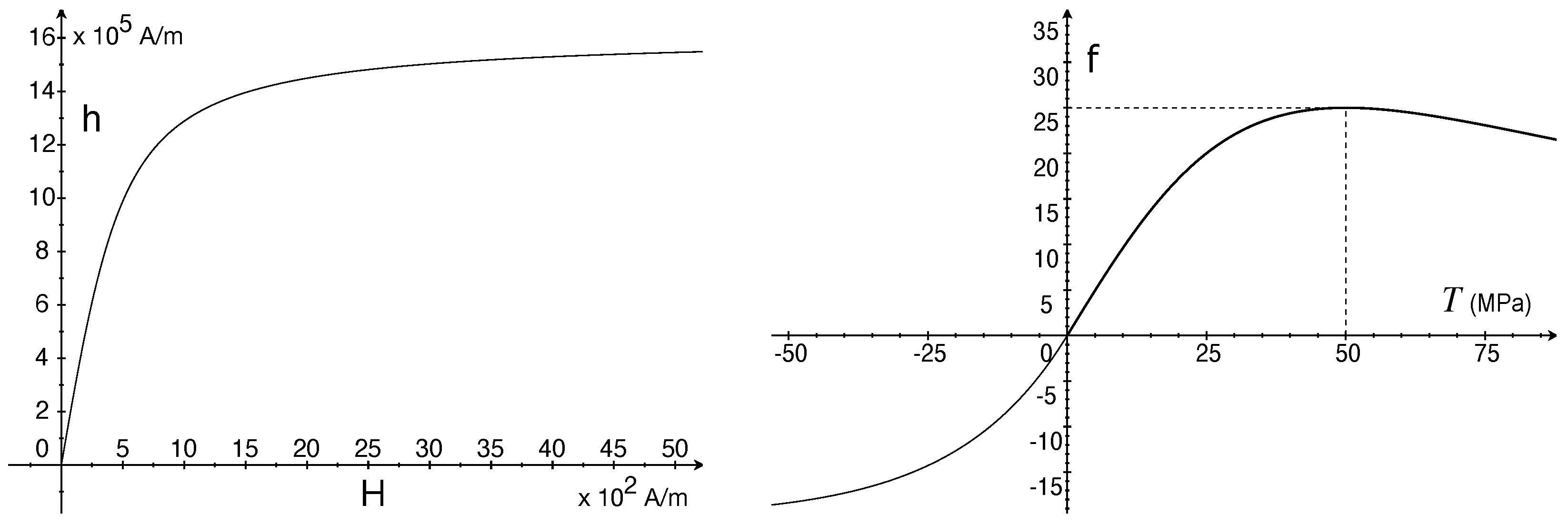
6. Models for Positive and Negative Magnetostriction

Especially in connection with magnetoelastic sensors and actuators, it is of interest to investigate the modeling of strain produced by a given stress (or stress impedance). As shown in the literature (e.g., [19,20,21] and refs therein), several effects connected with non-linearity, hysteresis, frequency dependence, and positive–negative magnetostriction occur. Here, we illustrate two aspects related to the sign of a magnetostriction. First, we show that different signs of a magnetostriction are obtained depending on the variable chosen to represent the interaction between deformation and the magnetic field.

If $\varphi$ depends on $\mathfrak{H}={\mathbf{F}}^T\mathsf{H}$, then it follows from the previous section that

$$\mathbf{T}+{\mu }_0\mathsf{H}\otimes \mathsf{M}=\rho \mathbf{F}{\mathsf{\partial }}_{\mathbf{E}}\varphi {\mathbf{F}}^T+\rho \theta {\gamma }_T\mathbf{D},{\mu }_0\mathsf{M}=\rho \mathbf{F}{\mathsf{\partial }}_{\mathfrak{H}}\varphi .$$

Assume that $\varphi$ depends on $\mathbf{E}$ through the quadratic scalar $\frac{1}{2}\mathbf{E}·\mathbb{C}\mathbf{E}$ where $\mathbb{C}$ is a symmetric fourth-order (elasticity) tensor. Hence, we can write

$$\rho \mathbb{C}\mathbf{E}={\mathbf{F}}^{-1}(\mathbf{T}+{\mu }_0\mathsf{H}\otimes \mathsf{M}-\rho \theta {\gamma }_T\mathbf{D}){\mathbf{F}}^{-T}.$$

Apart from the dissipative term $\rho \theta {\gamma }_T\mathbf{D}$, we conclude that the effective stress acting on the body is the sum $\mathbf{T}+{\mu }_0\mathsf{H}\otimes \mathsf{M}$.

Instead, we might take $\varphi$ as dependent on $\mathcal{H}={\mathbf{F}}^{-1}\mathsf{H}$. Since

$$\dot{\mathsf{H}}=\mathbf{L}\mathbf{F}\mathcal{H}+\mathbf{F}\dot{\mathcal{H}}$$

then substitution into

$$\mathbf{T}·\mathbf{L}-\rho {\mathsf{\partial }}_{\mathcal{H}}\varphi ·\dot{\mathcal{H}}-{\mu }_0\mathsf{M}·\dot{\mathsf{H}}-\rho \mathbf{F}{\mathsf{\partial }}_{\mathbf{E}}\varphi {\mathbf{F}}^T·\mathbf{D}$$

yields the thermodynamic inequality in the form

$$(\mathbf{T}-{\mu }_0\mathsf{M}\otimes \mathsf{H})·\mathbf{W}-(\rho {\mathsf{\partial }}_{\mathcal{H}}\varphi +{\mu }_0{\mathbf{F}}^T\mathsf{M})·\dot{\mathcal{H}}+(\mathbf{T}-{\mu }_0\mathsf{M}\otimes \mathsf{H}-\rho \mathbf{F}{\mathsf{\partial }}_{\mathbf{E}}\varphi {\mathbf{F}}^T)·\mathbf{D}+\dots =\theta {\gamma }_T{\left|\mathbf{D}\right|}^2,$$

with the dots representing terms independent of $\mathbf{W},\dot{\mathcal{H}},$ and $\mathbf{D}$. Hence, it follows that

$$\begin{array}{cc}& {\mu }_0{\mathbf{F}}^T\mathsf{M}=-\rho {\mathsf{\partial }}_{\mathcal{H}}\varphi ,\\ & \mathbf{T}-{\mu }_0\mathsf{M}\otimes \mathsf{H}\in \mathrm{Sym},\mathbf{T}-{\mu }_0\mathsf{M}\otimes \mathsf{H}=\rho \mathbf{F}{\mathsf{\partial }}_{\mathbf{E}}\varphi {\mathbf{F}}^T+\rho \theta {\gamma }_T\mathbf{D}.\end{array}$$

(52)

While

$$\mathbf{T}-{\mu }_0\mathsf{M}\otimes \mathsf{H}\in \mathrm{Sym}⟺\mathbf{T}+{\mu }_0\mathsf{H}\otimes \mathsf{M}\in \mathrm{Sym}$$

the effective stress turns out to be

$$\mathbf{T}-{\mu }_0\mathsf{M}\otimes \mathsf{H}$$

instead of $\mathbf{T}+{\mu }_0\mathsf{H}\otimes \mathsf{M}$. The difference is even more evident if we consider one-dimensional settings where the two stresses would be

$$T+{\mu }_0\mathsf{M}\mathsf{H},T-{\mu }_0\mathsf{M}\mathsf{H}.$$

In the first case, we recognize a positive magnetostriction, namely an additional term producing deformation due to the magnetic field; in the second one, there is a negative magnetostriction.

There are experimental data showing that a positive or negative magnetostriction in a given material depends on the value of the stress itself. This property is referred to as stress-impedance effect and has been observed experimentally in Co Fe Ni Mo B Si alloy [22] and Mn Zn Fe O ferrite [23]. In this connection, attention has been addressed to the Villari effect whereby the flux $\mathsf{B}$, for a given magnetic field, $\mathsf{H}$, depends on the applied stress in a non-monotonic way [24,25,26].

To clarify this point, we mention that, based on the data for NO Fe Si steel [24,25], we determined a thermodynamically-consistent one-dimensional model [27] where $\mathsf{M}$ is given the form

$$\mathsf{M}=\mathsf{h}\left(\mathsf{H}\right)+\mathsf{f}\left(T\right){\mathcal{K}}^{\prime }\left(\mathsf{H}\right);$$

(53)

$\mathsf{h}$ and $\mathcal{K}$ are positive functions of the applied magnetic field $\mathsf{H}$, with $\mathsf{h}\left(0\right)=\mathcal{K}\left(0\right)=0$, and $\mathsf{f}$ is a function of the stress T that has a maximum at $T=T_V>0$, with $T_V$ being referred to as a Villari point [28]; the functions $\mathsf{h},\mathsf{f}$, and $\mathcal{K}$ are plotted in Figure 1 and Figure 2.

Since ${\mu }_0\mathsf{M}=-\rho {\mathsf{\partial }}_{\mathsf{H}}\varphi$, then by the integration of (53), we have

$$\rho \varphi (\theta ,\mathsf{H},T)=\rho \tilde{\varphi }\left(\theta \right)-{\mu }_0\mathcal{H}\left(\mathsf{H}\right)-{\mu }_0\mathsf{f}\left(T\right)\mathcal{K}\left(\mathsf{H}\right)-\mathcal{T}\left(T\right)$$

where $\mathcal{H}$ is the primitive of $\mathsf{h}$. The thermodynamic condition

$$lnF=-{\mathsf{\partial }}_T\varphi$$

results in

$$lnF={\mu }_0{\mathsf{f}}^{\prime }\left(T\right)\mathcal{K}\left(\mathsf{H}\right)+{\mathcal{T}}^{\prime }\left(T\right).$$

The relative deformation (impedance) $lnF$ induced by the magnetic field is

$${(lnF)}_m={\mu }_0{\mathsf{f}}^{\prime }\left(T\right)\mathcal{K}\left(\mathsf{H}\right).$$

(54)

Since ${\mathsf{f}}^{\prime }\left(T\right)>0$ as $T<T_V$ and ${\mathsf{f}}^{\prime }\left(T\right)<0$ as $T>T_V$, then the sign of ${\mathsf{f}}^{\prime }\left(T\right)\mathcal{K}\left(\mathsf{H}\right)$ changes across $T=T_V$. Equation (54) shows that materials with a non-monotonic function, $\mathsf{f}$, (such as NO Fe-Si steel) can exhibit a change in sign of the magnetostrictive effect that depends on the applied stress.

7. Conclusions

The paper investigates some formulations of constitutive equations for electromagnetic solids subject to the constraint (14) that follows from the balance of angular momentum. Starting with a generic dependence of the free energy on the deformation gradient $\mathbf{F}$ and the magnetic field $\mathsf{H}$, it is shown in Section 5 that the two symmetry constraints (27), arising from thermodynamics and balance of angular momentum, lead to the condition (29) and indicate the dependence on the field

$$\mathfrak{H}={\mathbf{F}}^T\mathsf{H}$$

as the appropriate variable identically satisfying the two symmetry constraints. It then follows as a thermodynamic requirement that

$$\mathfrak{M}=J{\mathbf{F}}^{-1}\mathsf{M}$$

is the magnetization field conjugated to $\mathfrak{H}$. Incidentally, $\mathfrak{H}$ and $\mathfrak{M}$ are the magnetic field and the magnetization field often involved within modeling through Lagrangian fields. It is also shown that $\mathfrak{H}$ and $\mathfrak{M}$ are Euclidean invariants, which makes any function of $\mathfrak{H}$ and/or $\mathfrak{M}$ identically Euclidean-invariant. The same properties hold for the electric field $\mathfrak{E}={\mathbf{F}}^T\mathsf{E}$ and the polarization $\mathfrak{P}=J{\mathbf{F}}^{-1}\mathsf{P}$.

The symmetry condition (29) is found to hold even for the field $\mathcal{H}={\mathbf{F}}^{-1}\mathsf{H}$ which is also Eulerian-invariant. However, the field $\mathfrak{H}={\mathbf{F}}^T\mathsf{H}$ seems to be preferable in the literature in relation to its meaning as a Lagrangian field. Section 6 shows that ${\mathbf{F}}^T\mathsf{H}$ produces a positive magnetostriction, ${\mathbf{F}}^{-1}\mathsf{H}$ produces a negative magnetostriction.

No recourse is made to the splitting of the stress tensor as the sum of the mechanical stress and the magnetic (or electric) stress. In the balance equation, or symmetry condition,

$$\mathbf{T}+{\mu }_0\mathsf{H}\otimes \mathsf{M}\in \mathrm{Sym}$$

the stress tensor $\mathbf{T}$ is the stress within the body which has to balance the skew part of ${\mu }_0\mathsf{H}\otimes \mathsf{M}$. This avoids non-uniqueness problems and questions the appropriate form of the magnetic stress.

Among the results obtained, we mention that, for elastic solids, it follows from thermodynamics that the stress tensor $\mathbf{T}$ has the form

$${\mathbf{T}}^e=-{\mu }_0\mathsf{H}\otimes \mathsf{M}+\rho \mathbf{F}{\mathsf{\partial }}_{\mathbf{F}}\varphi {\mathbf{F}}^T,$$

where the free energy $\varphi$ is a function of the temperature $\theta$, the strain $\mathbf{E}$, and the magnetic field $\mathfrak{H}$. Further, upon the use of a representation formula for vectors and tensors, the thermodynamic reduced conditions are investigated to determine the dissipative stress $\mathbf{T}-{\mathbf{T}}^e$ and the rate $\dot{\mathbf{q}}$. It is of interest that there is the allowed dependence on the stretching $\mathbf{D}$ in the form (47), namely

$$\mathbf{T}={\mathbf{T}}^e+\left(\rho \theta {\gamma }_T-\beta {\displaystyle \frac{\mathsf{H}·\mathbf{D}\mathsf{H}}{{\left|\mathbf{D}\right|}^2}}\right)\mathbf{D}+\beta \mathsf{H}\otimes \mathsf{H},$$

where $\beta$ and ${\gamma }_T$ are functions of the temperature and the strain. The analogous application of the representation formula for the terms involving the heat flux results in a family of evolution equations among which the Maxwell–Cattaneo equation is obtained.

References

1. Fano, R.M.; Chu, L.J.; Adler, R.B. Electromagnetic Fields, Energy, and Forces; MIT Press: Cambridge MA, USA, 1968. [Google Scholar]
2. Maugin, G.A. Continuum Mechanics of Electromagnetic Solids; North-Holland: Amsterdam, The Netherlands, 1988. [Google Scholar]
3. Pao, Y.-H.; Hutter, K. Electrodynamics for moving elastic solids and viscous fluids. Proc. IEEE 1975, 63, 1011–1021. [Google Scholar]
4. Dorfmann, L.; Ogden, R.W. The nonlinear theory of magnetoelasticity and the role of the Maxwell stress: A review. Proc. R. Soc. A 2023, 479, 592. [Google Scholar] [CrossRef]
5. Spaldin, N.A. A beginner’s guide to the modern theory of polarization. J. Solid State Chem. 2012, 195, 2–10. [Google Scholar] [CrossRef]
6. Griffiths, D.J. Introduction to Electrodynamics; Cambridge University Press: Cambridge, UK, 2024. [Google Scholar]
7. Gurtin, M.E.; Fried, E.; Anand, L. The Mechanics and Thermodynamics of Continua; Cambridge University Press: Cambridge, UK, 2010. [Google Scholar]
8. Kovetz, A. Electromagnetic Theory; Oxford University Press: Oxford, UK, 2000. [Google Scholar]
9. Morro, A.; Giorgi, C. Mathematical Methods of Continuum Physics; Birkhäuser: Cham, Switzerland, 2023. [Google Scholar]
10. Bustamante, R.; Dorfmann, A.; Ogden, R.W. On electric body forces and Maxwell stresses in nonlinearly electroelastic solids. Int. J. Eng. Sci. 2009, 47, 1131–1141. [Google Scholar] [CrossRef]
11. Bustamante, R.; Rajagopal, K.R. On a new class of electroelastic bodies. I. Proc. R. Soc. A 2013, 469, 521–536. [Google Scholar] [CrossRef]
12. Dorfmann, A.; Ogden, R.W. Nonlinear magnetoelastic deformations. Q. J. Mech. Appl. Math. 2004, 57, 599–622. [Google Scholar] [CrossRef]
13. Saxena, P.; Hossain, M.; Steinmann, P. Nonlinear magneto-viscoelasticity of transversally isotropic magnetoactive polymers. Proc. R. Soc. A 2014, 470, 82–104. [Google Scholar] [CrossRef]
14. Müller, I. On the entropy inequality. Arch. Ration. Mech. Anal. 1967, 26, 118–141. [Google Scholar] [CrossRef]
15. Casas-Vázquez, J.; Jou, D. Temperature in non-equilibrium states: A review of open problems and current proposals. Rep. Prog. Phys. 2003, 66, 1937–2023. [Google Scholar] [CrossRef]
16. Gujrati, P.D. Irreversibility, dissipation, and its measure. Symmetry 2025, 17, 232. [Google Scholar] [CrossRef]
17. Dorfmann, L.; Ogden, R.W. Hard-magnetic soft magnetoelastic materials: Energy considerations. Int. J. Solids Struct. 2024, 294, 112789. [Google Scholar] [CrossRef]
18. Straughan, B. Heat Waves; Springer: Berlin/Heidelberg, Germany, 2011. [Google Scholar]
19. Gazda, P.; Nowicki, M.; Szewczyk, R. Comparison of stress-impedance effect in amorphous ribbons with positive and negative magnetostriction. Materials 2019, 12, 275. [Google Scholar] [CrossRef]
20. Bienkowski, A. Magnetoelastic Villari effect in Mn-Zn ferrites. J. Magn. Magn. Mater. 2000, 215, 231–233. [Google Scholar] [CrossRef]
21. Narita, F.; Fox, M.A. A review on piezoelectric, magnetostrictive, and magnetoelectric materials and device technologies for energy harvesting applications. Adv. Eng. Mater. 2018, 20, 1700743. [Google Scholar] [CrossRef]
22. Gazda, P.; Nowicki, M. Giant stress-impedance effect in CoFeNiNoBSi alloy in variation of applied magnetic field. Materials 2021, 14, 1919. [Google Scholar] [CrossRef]
23. Bieńkowski, A.; Kulikowski, J. Effect of stresses on the magnetostriction of Ni-Zn(Co) ferrites. J. Magn. Magn. Mater. 1991, 101, 122–124. [Google Scholar] [CrossRef]
24. Daniel, L.; Rekik, M.; Hubert, O. A multiscale model for magneto-elastic behaviour including hysteresis effects. Arch. Appl. Mech. 2014, 84, 1307–1323. [Google Scholar] [CrossRef]
25. Hubert, O. Multiscale magneto-elastic modeling of magnetic materials including isotropic second order stress effect. J. Magn. Magn. Mater. 2019, 491, 165564. [Google Scholar] [CrossRef]
26. Szewczyk, R. Stress-induced anisotropy and stress dependence of saturation magnetostriction in the Jiles-Atherton-Sablik model of the magnetoelastic Villari effect. Arch. Metall. Mater. 2016, 61, 607–612. [Google Scholar] [CrossRef]
27. Giorgi, C.; Morro, A. On the Modelling of Magneto-Mechanical Effects in Solids. Available online: https://papers.ssrn.com/sol3/papers.cfm?abstract_id=4750363 (accessed on 6 May 2024).
28. Riesgo, G.; Elbaile, L.; Carrizo, J.; Crespo, R.D.; García, M.Á.; Torres, Y.; García, J.Á. Villari effect at low strain in magnetoactive materials. Materials 2020, 13, 2472. [Google Scholar] [CrossRef] [PubMed]
29. Dorfmann, L.; Ogden, R.W. Nonlinear electroelasticity: Material properties, continuum theory and applications. Proc. R. Soc. A 2017, 473, 311. [Google Scholar] [CrossRef] [PubMed]
30. Wang, B.; Kari, L. Constitutive model of isotropic magneto-sensitive rubber with amplitude, frequency, magnetic and temperature dependence under a continuum mechanics basis. Polymers 2021, 13, 472. [Google Scholar] [CrossRef] [PubMed]
31. Mehnert, M.; Hossain, M.; Steinmann, P. Numerical modeling of thermo-electro-viscoelasticity with field-dependent material parameters. Int. J. Non-Linear Mech. 2018, 106, 13–24. [Google Scholar] [CrossRef]
32. Giorgi, C.; Morro, A. Electrostriction and modelling of finitely deformable dielectrics. Acta Mech. 2024, 236, 229–240. [Google Scholar] [CrossRef]
Figure 1. Plots of h ( H ) (left) and f ( T ) with T V = 50 MPa (right).
Symmetry 17 00557 g001
Figure 2. Plots of K ( H ) , with H 0 = 6 · 10 3 A/m (solid line) and K ( H ) (dashed line).
Symmetry 17 00557 g002
Disclaimer/Publisher’s Note: The statements, opinions and data contained in all publications are solely those of the individual author(s) and contributor(s) and not of MDPI and/or the editor(s). MDPI and/or the editor(s) disclaim responsibility for any injury to people or property resulting from any ideas, methods, instructions or products referred to in the content.