Target Enclosing Control of Symmetric Unmanned Aerial Vehicle Swarms Based on Crowd Entropy

Abstract

Drone swarms often need to fly cooperatively in complex spaces filled with multiple obstacles. In such scenarios, they must meet the requirements of both external obstacle avoidance and internal collision avoidance while maintaining a certain topological configuration among individuals. This easily leads to problems such as congestion, oscillation, and poor stability, including being out of control. Thus, it is essential to measure system-wide stability, regulate the autonomous cooperative evolution of swarms, and enhance their adaptation to environmental changes. To solve this problem, using the symmetric unmanned aerial vehicle (UAV) swarm as the research object, a group entropy measurement theory for the stability of drone swarms is proposed. We introduce an entropy-based metric for group motion consistency. This metric serves as a fitness index for individual collaboration, enabling adaptive adjustment of drone swarm coherence under multi-obstacle conditions. Finally, simulation experiments are conducted to verify the effectiveness of the established theory and algorithm.

1. Introduction

Drone swarms are widely used in fields such as urban combat and search and rescue due to their advantages of low cost, large scale, and high synergy [1,2]. An increasing number of flight missions require drones to operate in clusters within complex, dynamic environments—such as urban canyons, mountainous terrain, and forests. [3,4]. However, in these environments, there are uncertain factors, such as complex and changeable obstacles, as well as limited communication and sensing capabilities of drones, making it difficult for the current methods based on preset group motion behavior control to quickly and dynamically adjust to adapt to environmental changes [5,6]. At the same time, factors such as system delays and cumulative errors in sensors are difficult to avoid, causing the swarm system to be difficult to track the preset state and leading to the failure of swarm control based on preset behaviors [7]. Therefore, how to measure the stability degree of the entire system and regulate the autonomous, rapid cooperative evolution of the swarm, as well as its adaptation to environmental and situational changes, is still a problem worthy of research in the field of intelligent drone swarms.

Andrea Cavagna and Asja Jelic from the Institute for Complex Systems in Rome studied a new model of bird flock convergence [8]. The new model is the same as the equation describing superfluid helium. When the temperature is close to absolute zero, helium becomes a superfluid with no viscosity at all. At this time, the superfluid is governed by the laws of quantum physics. Each atom in the superfluid shares the same quantum state, which has mathematical similarities to bird flocks [9].

In the 2023 Nature Physics article collection, Yu-Hai Tu, a researcher at the IBM T. J. Watson Research Center in the United States, used the renormalization method to study the phase transition theory of the configuration of natural swarm dynamic systems. This research revealed that there is a phase transition phenomenon in the configuration of biological swarms that is very similar to the solid–liquid–gas three-state switching of water [10]. These findings help to identify the “key” to regulating the phase transition of a large number of swarm configurations in nature and thus open the door to the active regulation of swarms of unmanned systems (drones, unmanned boats, unmanned vehicles, etc.).

The phase state changes occurring during the flight process of unmanned system swarms in space provide a basis for the application of theories of fluid mechanics in the field of unmanned swarm modeling, making it possible to solve the problems of fluidity and maneuverability of drone swarms in confined spaces. However, which theoretical tool to use to measure the dynamic characteristics, such as density and velocity of group flow, remains to be further solved. As a profound scientific concept for complexity measurement, entropy can effectively measure the dynamic characteristics of swarm intelligence [11] and characterize it. It can not only measure the degree of chaos and uncertainty of group behavior and associated structures in a statistical sense, but also measure the dynamic complexity characteristics and structural complexity in the process of swarm intelligence formation, and determine the complexity of the final form of evolution [12].

To address the motion stability of drone swarms in complex flight environments, this paper establishes a metric for quantifying swarm motion stability. Based on this metric, dynamic adjustments to swarm model parameters are implemented to maintain motion coherence under time-varying external disturbances. The team of Haibin Duan from Beihang University has conducted in-depth research on the group entropy measurement problem in swarm intelligence systems. Jie Luo et al. proposed the basic characteristics of swarm intelligence systems and their excitation and convergence modeling [13], pointing out that swarm intelligence systems are essentially a kind of complex nonlinear dynamic system. They also proposed the essential properties required for valid group entropy metrics in such systems. Lin Chen et al. proposed a distributed swarm target encirclement control method based on local metric distance interaction for the problem of target encirclement control of drone swarms in a constrained environment [14], achieving drone swarm control based on entropy measurement. From the above work, it can be seen that the group entropy measurement in drone swarms has scientific feasibility and high adaptive adjustment ability.

This paper proposes a group entropy measurement theory for the motion consistency of drone swarms. An entropy measurement function for the stability degree of group motion behavior is established. The entropy measurement function is used as an index of fitness value for collaborative movement among individuals. Adaptive adjustment of the motion consistency of drone swarms in complex environments is realized. Since intelligence itself is an abstract entity and it is difficult to evaluate and measure it directly, the behavior of a swarm intelligence system serves as the external manifestation of swarm intelligence, a phenomenon that can be directly measured. Therefore, we can start with the dynamic behavior of the system and explore the measurement theories and methods of swarm intelligence systems.

The flowchart of the experimental design of this paper is shown as follows in Figure 1. Starting from the challenges faced by the flight of the unmanned aerial vehicle (UAV) swarm in complex environments, the theory of swarm entropy measurement is introduced. This theory is used to address the stability issue of the UAV swarm during flight. Based on this theory, a swarm model is constructed and improved, which covers the analysis of the characteristics of symmetric UAVs, as well as the establishment and refinement of multiple models. The improved model is comprehensively verified through three types of experiments, namely algorithm verification, physical simulation, and physical prototyping. By analyzing the experimental data, research conclusions are drawn, clarifying the effectiveness and limitations of the theory of swarm entropy measurement, thus determining future research directions.

1.1. Symmetric Unmanned Aerial Vehicle (UAV) Swarms

In a symmetric UAV swarm, each UAV has basically the same hardware configuration and performance parameters, such as model type, flight speed, endurance, payload capacity, etc. This endows them with similar capabilities and behavioral patterns when performing tasks. For example, in some simple area monitoring tasks, multiple quadrotor UAVs of the same model can have task assignments in a symmetric manner. These coordinated agents systematically inspect designated zones through synchronized flight trajectories and identical scanning frequencies, thereby establishing equilibrium in workload distribution.

The advantage of a symmetric swarm lies in its relatively simple control strategy, which is easy to plan and manage uniformly. The inherent hardware compatibility among swarm members enhances synchronization precision and collaborative efficiency during cooperative operations. For some routine and repetitive target encirclement tasks, these can be completed efficiently. However, the limitation of a symmetric swarm is its lack of flexibility. It is difficult to cope with complex, changeable task scenarios with special requirements. Any operational parameters exceeding preconfigured system thresholds will substantially compromise the collective effectiveness of the swarm, particularly when encountering scenarios requiring adaptive decision-making.

1.2. Kinematic Model of Symmetric UAV Swarms

This study focuses on quadrotor unmanned aerial vehicles (UAVs), which exhibit fundamentally different motion characteristics from fixed-wing UAVs due to their vertical takeoff and landing (VTOL) capabilities. To simplify the dynamic modeling, the pitch angle of the quadrotor is disregarded, and only its current altitude is considered as the primary state variable. Based on a symmetric swarm system composed of N drones in three-dimensional Euclidean space, a kinematic model of drones under the inertial reference frame coordinates can be established:

$$\begin{array}{l}{\dot{x}}_i=V_i\cos {\omega }_i\\ {\dot{y}}_i=V_i\sin {\omega }_i\\ {\dot{z}}_i=h_i\end{array}$$

(1)

The subscript $i\in N$ in Equation (1) denotes the first UAV in the cluster, ${\omega }_i$ is the angle between the horizontal velocity vector of the first UAV and the X-axis of the inertial coordinate system, $h_i$ is the flight altitude of the $i$th UAV, and $V_i={[{\dot{x}}_i,{\dot{y}}_i,{\dot{z}}_i]}^{\mathrm{T}}$ is the velocity vector of the $i$th UAV.

In the current model, angular dynamics are restricted to the XY-plane, thereby enabling focused investigation into the regulatory role of swarm entropy on motion consensus in 2D formations, as well as the design and validation of associated decentralized algorithms.

Defined $P_i={[{\dot{x}}_i,{\dot{y}}_i,{\dot{z}}_i]}^{\mathrm{T}}$ as the position vector of the $i$th drone. Considering that the drone is constrained by the communication and perception capabilities in the real flight environment, the sensing range of the drone is defined as a spherical field with a radius $R_c$. For any drone $i\in N$, other drone sets $N_j^{neighbour}$ and obstacle sets $N_j^{obst}$ within the sensing range of the $i$th drone can be expressed:

$$N_j^{neighbour}=\{j:||P_i-P_j||<2R_c,i\in N,j\in N\wedge j\ne i\}$$

(2)

$$N_j^{obst}=\{j:||P_i^{obst}-P_i||<R_c,j\in N\wedge j\ne i\}$$

(3)

In Equations (2) and (3), $P_i$ and $P_j$ represent the positions of UAVs $i$ and $j$ in the swarm, respectively. $P_i^{obst}$ is the projection position of the UAV $N_i$ on the obstacle.

Regarding the velocity calculation method within the sensing and communication range of individual UAVs, each UAV’s velocity vector is decomposed into components for internal collision avoidance, velocity alignment, obstacle avoidance, and self-propulsion into four components [15]. Below, we provide the velocity calculation model for each part.

• Internal Collision Avoidance Component Model

For any UAV $N_i$ within the sensing range $R_c$ of UAV $N_j^{neighbour}$, there is a mutual repulsive force with an effective radius of $r^{rep}$ to ensure that there is no internal collision within the UAV swarm. Hence, the velocity component formula for swarm internal collision avoidance [16] is established as follows:

$$v_{ij}^{rep}=p^{rep}\cdot (r^{rep}-r_{ij})\cdot {\displaystyle \frac{r_i-r_j}{r_{ij}}}$$

(4)

In Equation (4), $p^{rep}$ represents the linear growth of the repulsive force, and $r_{ij}=\left|\right|r_i-r_j\left|\right|$ is the positional difference between UAV $N_i$ and UAV $N_j$. When the distance between UAVs in the swarm is smaller than the effective radius of repulsion, i.e., $r_{ij}<r^{rep}$, the internal collision avoidance velocity component is calculated according to Equation (4). If $r_{ij}⩾r^{rep}$, the internal collision avoidance velocity component of UAVs is ignored.

2

Velocity Alignment Component Model

The proposed negative feedback-adjusted velocity component induces progressive velocity synchronization across the UAV cluster through iterative updates of the velocity calculation model, as formalized in Equation (5):

$$\begin{array}{l}{v}_{ij}^{frict\max }=\max (v^{frict},D(r_{ij}-d^{pros},a^{frict},p^{frict}))\\ v_{ij}^{frict}=C^{frict}(v_{ij}-v_{ij}^{frict\max })\cdot {\displaystyle \frac{v_i-v_j}{v_{ij}}}\end{array}$$

(5)

In Equation (5), $v_{ij}$ represents the velocity difference between UAV $i$ and UAV $j$, and $v_{ij}^{frict}$ represents the velocity alignment component. $v_{ij}^{frict\max }$ is used to calculate the maximum velocity alignment error, $d^{pros}$ represents the expected distance between UAVs, $C^{frict}$ is the linear gain for velocity alignment, and $v^{frict}$ is the allowable error for velocity alignment. When the distance between UAVs in the swarm is greater than the effective radius, the velocity alignment component is calculated as shown in Equation (5); otherwise, it is ignored. $a^{frict}$ is the preferred acceleration, and $p^{frict}$ is used to determine the linear gain at the crossover point of the two deceleration phases. $D(·)$ is the decay function designed for the smooth transition of velocity between the two states, and the calculation formula is shown in Equation (6):

$$D(r,a,p)=\left\{\begin{array}{c}0\\ rp\\ \sqrt{2ar-a^2/p^2}\end{array}\right.$$

(6)

In Equation (6), p ≠ 0, $r$ represents the distance between the UAV and the expected stop point, $a$ is the initial acceleration, and $p$ is used to determine the linear gain at the crossover point of the two deceleration phases. When $r<0$, $D(·)$ = 0; when $0<rp<a/p$, $D(·)$ is calculated as $rp$; in other cases, $D(·)$ is calculated as $\sqrt{2ar-a^2/p^2}$.

3

Obstacle Avoidance Component Model

The obstacle avoidance component adopts a methodology similar to that of the velocity alignment calculation. By treating obstacles as virtual UAVs without velocity tolerance errors, collision avoidance is achieved through the velocity alignment framework. Define the virtual UAV’s position vector as $P_i^o={[x_i^o,y_i^o,z_i^o]}^{\mathrm{T}}$, and the velocity vector as $v_i^o={[{\dot{x}}_i^o,{\dot{y}}_i^o,{\dot{z}}_i^o]}^{\mathrm{T}}$. The obstacle avoidance velocity component is then calculated [17], as shown in Equation (7):

$$\begin{array}{l}{v}^{obst\max }=D(r_{is}-r_o^{obst},a^{obst},p^{obst})\\ v^{obst}=v_{is}^{frict}(C-1)=(v_{is}-v^{obst\max })\cdot {\displaystyle \frac{v_i-v_i^o}{v_{is}}}\end{array}$$

(7)

In Equation (7), the function $D(·)$ is calculated similarly to Equation (6). $r_{is}=\left|\right|P_i-P_i^o\left|\right|$ is the positional difference between the UAV and the virtual UAV, and $v_{is}=\left|\right|v_i-v_i^o\left|\right|$ is the velocity difference between the UAV and the virtual UAV. Unlike the velocity alignment formula, the virtual UAV does not have a velocity tolerance error. When the UAV-obstacle distance exceeds the effective radius, the collision avoidance velocity component is computed via Equation (7); otherwise, this component is deactivated.

4

Self-propelled component model

When the speed of the UAV is zero, the cluster model will fall into a local optimal solution and lead to cluster failure. Therefore, a self-propulsion term that maintains the current speed is added to the speed component, and a parameter is set to control its size.

5

Multi-UAV Distributed Cluster Modeling

A distributed UAV cluster model is constructed by integrating the four aforementioned components. The velocity calculation for the i-th UAV is formalized in Equation (8):

$$\begin{array}{l}{v}_i^d={\alpha }^{rep}\cdot {\displaystyle \sum _j{v}_i^{rep}}+{\alpha }^{frict}\cdot {\displaystyle \sum _j{v}_i^{frict}}+\\ \hspace{1em}\hspace{1em}{\alpha }^{obst}\cdot {\displaystyle \sum _j{v}_i^{obst}}+{\alpha }^{iner}\cdot {\displaystyle \frac{v_i}{\left|v_i\right|}}{v}^{iner}\end{array}$$

(8)

In Equation (8) ${\alpha }^{rep}$, ${\alpha }^{frict}$, ${\alpha }^{obst}$ and ${\alpha }^{iner}$ are the weights of each velocity component. Based on the velocity calculation formula of each UAV, the UAV-distributed cluster control strategy can be designed as follows:

$$\begin{array}{l}\underset{t\to \infty }{\lim }\left|\right|P_i-P_j\left|\right|=d^{pros}\\ \underset{t\to \infty }{\lim }\left|\right|v_i-v_j\left|\right|<v^{frict}\\ \left|\right|P_i-P_i^o\left|\right|>r_{is}\end{array}$$

(9)

Through iterative algorithm updates, the swarm evolves into a distributed system characterized by stable inter-agent spacing, velocity consensus, and autonomous obstacle navigation. Compared with the traditional UAV-distributed cluster model, the above UAV-distributed cluster model omits the cohesive effect that brings UAVs close to one another. While resolving system oscillations from gravitational–repulsive force interactions among UAVs, this modification introduces cluster dispersion vulnerability under external disturbances. The speed of a UAV is jointly determined by its current speed, the speed of other UAVs within its sensing range, and the influence of obstacles. The UAV’s speed will produce a large amount of randomness when encountering a more complex external disturbance, leading to the dispersion of the originally clustered UAV group. The stochasticity in this model stems from external disturbances, where all external entities except the UAVs themselves are classified as obstacles. To maintain planar motion tractability, quadrotors only perceive obstacles that are coplanar with their horizontal plane, and their collision avoidance dynamics exclusively consider horizontal velocity components. Consequently, the induced stochasticity remains confined to the 2D translational domain. To address this limitation, we propose a swarm entropy metric theory for motion consistency, which realizes adaptive regulation of UAV cluster motion consistency under complex environments by establishing the entropy metric function of the stability degree of the group motion behavior and taking it as the adaptive value indicator of the coordinated motion between individuals.

2. Unmanned Aerial Vehicle Cluster Model Based on Group Entropy Measurement

2.1. Adaptation Value Interaction Mechanism

The velocity alignment component incorporates the averaged velocities of neighboring UAVs within the communication range, with influence weights dynamically scaled by their relative distances to the central agent. Therefore, in this paper, we improve the calculation of speed alignment by converting the fitness value into the influence weight of each UAV in the speed alignment component. Through rigorous fitness metric design, UAVs autonomously identify optimal behavioral patterns from high-fitness neighbors during swarm coordination. The velocity alignment mechanism fundamentally governs inter-UAV influence, driving convergence toward uniform velocity magnitude and direction across the swarm. The result of velocity alignment is that the UAVs will maintain the formation of the cluster, but the direction of the overall flight of the cluster has greater randomness and fluctuates more under external noise interference. This vulnerability stems from the equivalent weighting of all perceived neighbors in velocity calculations. In the iterative process of the clustering algorithm, the main influence on the results of the speed alignment calculation is the speed difference between the UAVs, i.e., the speeds of the UAVs will tend to align with those UAVs that have a larger speed difference within their sensing range. Consequently, swarm velocity biases toward faster outliers become susceptible to noise-induced divergence from collective motion consistency.

In order to achieve motion consistency within the UAV swarm, the velocity alignment component incorporates the influence of weight $N_j$ for each $p^{fitness}$. The modified velocity alignment [18] formula is shown in Equation (10):

$$\begin{array}{l}{v}_{ij}^{frict\max }=\max ({\tilde{v}}^{frict},D(r_{ij}-d^{pros},a^{frict},p^{frict}))\\ {\tilde{v}}_{ij}^{frict}=p_{ij}^{fitnesss}\cdot C^{frict}(v_{ij}-v_{ij}^{frict\max })\cdot {\displaystyle \frac{v_i-v_j}{v_{ij}}}\end{array}$$

(10)

In Equation (10), $p_{ij}^{fitness}$ represents the influence weight of UAV $N_j$ within the sensing range of UAV $N_i$ in the velocity alignment formula. It is calculated based on the fitness value of the UAV $N_j$ relative to all UAVs within the sensing range of UAV $N_i$. The specific calculation of $p_{ij}^{fitness}$ is shown in Equation (11):

$$\left\{\begin{array}{l}{p}_{ij}^{fitness}={\displaystyle \frac{p_j^{fitness}+C^{conver}}{{\displaystyle \sum _j{p}_j^{firtness}+p_i^{fitness}}}}\\ C^{conver}={\displaystyle \frac{p_i^{fitness}}{N_i^{number}}}\end{array}\right.$$

(11)

In Equation (11), $p_i^{fitness}$ represents the fitness value of UAV $N_i$, and $p_j^{fitness}$ represents the fitness value of UAV $N_j$. $C^{conver}$ ensures that the final velocity of the UAV swarm converges toward stability. $N_i^{number}$ is the number of other UAVs within the sensing range of UAV $i$. The updated velocity calculation formula is shown in Equation (12):

$$\begin{array}{l}{\tilde{v}}_i^d={\alpha }^{rep}\cdot {\displaystyle \sum _j{v}_i^{rep}}+{\alpha }^{frict}\cdot {\displaystyle \sum _j{\tilde{v}}_i^{frict}}+\\ \hspace{1em}\hspace{1em}{\alpha }^{obst}\cdot {\displaystyle \sum _j{v}_i^{obst}}+{\alpha }^{iner}\cdot {\displaystyle \frac{v_i}{\left|v_i\right|}}{v}^{iner}\end{array}$$

(12)

In the velocity alignment component, a parameter $C^{conver}$ is introduced to ensure that the velocity friction component ${\tilde{v}}_i^{frict}$ does not significantly increase or decrease, preventing the swarm system from losing control. In Equation (12), when $v_{ij}>v_{ij}^{frict\max }$, and only considering velocity magnitude issues, the parameter $p_{ij}^{fitness}$ is analyzed for its impact on the velocity friction component ${\tilde{v}}_i^{frict}$:

$$\begin{array}{l}{\displaystyle \sum _j{\tilde{v}}^{frict}}={\displaystyle \sum _j{p}_{ij}^{fitness}\cdot C^{frict}\cdot (v_{ij}-v_{ij}^{frict\max })\cdot \frac{v_i-v_j}{v_{ij}}}=\\ \hspace{1em}\hspace{1em}\hspace{1em}\hspace{1em}{\displaystyle \sum _j\frac{p_j^{fitness}+C^{conver}}{{\displaystyle \sum _j{p}_j^{fitness}+p_i^{fitness}}}}\cdot C^{frict}\cdot (v_{ij}-v_{ij}^{frict\max })\cdot {\displaystyle \frac{v_i-v_j}{v_{ij}}}=\\ \hspace{1em}\hspace{1em}\hspace{1em}\hspace{1em}{\displaystyle \sum _j\frac{p_j^{fitness}+\frac{p_i^{fitness}}{N_j^{number}}}{{\displaystyle \sum _j{p}_j^{fitness}+p_i^{fitness}}}}\cdot C^{frict}\cdot (v_{ij}-v_{ij}^{frict\max })\cdot {\displaystyle \frac{v_i-v_j}{v_{ij}}}=\\ \hspace{1em}\hspace{1em}\hspace{1em}\hspace{1em}{C}^{frict}\cdot (v_{ij}-v_{ij}^{frict\max })\end{array}$$

In the overall velocity synthesis formula, the introduction of the parameter $C^{conver}$ allows for changes in the influence weight of UAV $N_j$ on UAV $N_i$, without significantly increasing or decreasing the velocity alignment component. Such design constraints prevent velocity accumulation artifacts in alignment computations. Our directional selection refinement ensures strict velocity magnitude synchronization across the swarm.

2.2. Group Entropy Measurement of Motion Consistency

With the development of information theory and cybernetics, the concept of entropy has been gradually introduced into the evaluation of multi-intelligent body systems in recent years and is used to express the degree of chaos and disorder of the system. Entropy increase indicates the tendency of the system to evolve to a chaotic and disordered state, and entropy decrease indicates the tendency of the system to evolve into a harmonious and orderly state. Group entropy is defined as a composite function of the entropy of the system structure and the entropy of the information [19] of individual interactions:

$$E=F\circ G(\ln [\mathsf{\Xi }])$$

(13)

In Equation (13), $G$ is the evolution function reflecting the individual structure’s degree of dissipation, and $F$ is the evolution function reflecting the overall system’s level of coordinated dissipation. The function $F\circ G$ represents the composite operation of $F$ and $G$, and $\ln [\mathsf{\Xi }]$ is the statistical significance of group behavior at a given moment for a single individual.

When UAV clusters fly in complex environments, they need to constantly change their flight direction to achieve obstacle traversal and the motion consistency of each UAV in the cluster gradually decreases over time. The motion consistency of UAV clusters is difficult to assess and measure directly, while the velocity samples of UAVs in cluster motion are the external manifestation of motion consistency, which is a variable that can be practically measured and controlled [20]. Therefore, it is advisable to establish a group entropy metric system based on the velocity samples of each UAV to regulate the motion consistency level of the UAV cluster system in the complex flight environment.

Equation (13) is specifically applied to the local velocity dissipation of a UAV swarm, denoted as Section 2.1 In the velocity alignment calculation formula, a reasonable influence weight parameter $p_{ij}^{fitness}$ is introduced. In Section 2, the definition of $N_j^{neighbour}$ is provided, based on which the communication range $R_c$ can be used to divide the swarm into $K$ different subgroups, with the subgroup’s division changing over time. For each UAV $N_i$, every UAV within its sensing range forms its own center subgroup. Define that at time $t$, UAV $N_j$ is the center of the subgroup $Q_{N_j}^t$, and for the velocity of all UAVs in the subgroup, the smaller the velocity difference, the smaller the dissipation degree of the corresponding subgroup. In the expected distributed swarm system, each UAV’s velocity should be within a certain tolerance range $v^{frict}$, meaning that the fitness value of the subgroup $Q_{N_j}^t$ remains within a core range. This paper uses the velocity alignment parameter to achieve velocity dissipation control between UAV subgroups, thereby maintaining the stability of the UAV swarm.

This paper uses the variance of the velocity samples to describe the degree of velocity difference within UAV subgroups. A subgroup $Q_{N_j}^t$ of the UAV swarm contains each UAV’s velocity, forming a dataset sample $X_j^t$, with its variance denoted as $D_j^t$. As the calculation evolves, the aim is for the UAV swarm to trend toward a convergent swarm, ensuring that the velocities of all UAVs within the swarm become consistent, and the variance of the velocity samples decreases, as described by Equation (14):

$$\underset{t\to \infty }{\lim }{D}_i^t=\min (D_j^t),\forall N_j^t\in Q_{N_j}^t$$

(14)

In Equation (14), $D_j^t$ represents the variance of the velocity sample of the subgroup $N_i$ at time $t$, and $N_j^t$ represents the subgroup formed with UAV $N_i$ as the center at time t. According to the calculation of dissipation in Equation (13), the local velocity dissipation $E_v$ for subgroup $Q_{N_j}^t$ is defined as follows:

$$E_v={\displaystyle \sum _{Q_{N_j}^t}(D_j^t\cdot {\log }_2{D}_j^t)}$$

(15)

In the process of UAV clustering, the system is iteratively optimized toward the trend of entropy reduction. During the iteration of the algorithm, the weight of the influence of the clusters $Q_{N_j}$, which have smaller speed differences, on the clusters $Q_{N_i}$ is increased, so the inverse of the entropy is chosen as the fitness value for the interaction between the drones, i.e.,

$$p_j^{fitness}={\displaystyle \frac{1}{E_v}}$$

(16)

Summarizing the work in Section 2.1 and Section 2.2, the velocity alignment equation in the improved UAV cluster model is shown in Equation (17):

$$\begin{array}{l}{v}_{ij}^{frict\max }=\max (v^{frict},D(r_{ij}-d^{pros},a^{frict},p^{frict}))\\ {\tilde{v}}_{ij}^{frict}={\displaystyle \frac{1}{{\displaystyle \sum _{Q_{N_j}^t}\{D_j^t\cdot {\log }_2(D_j^t)\},}}}\cdot C^{frict}(v_{ij}-v_{ij}^{frict\max })\cdot {\displaystyle \frac{v_i-v_j}{v_{ij}}}\end{array}$$

(17)

Equation (17), in which ${\tilde{v}}_{ij}^{frict}$ is the UAV cluster speed alignment calculation formula based on the group entropy metric.

Aiming at the group entropy metric for the consistency of UAV cluster motion in a complex environment, the adaptive regulation of the weight of UAV influence on the surrounding subgroups during the clustering process is achieved through the improvement of the speed alignment algorithm in the clustering model to ensure the consistency of UAV cluster motion.

System stability analysis

An in-depth analysis of the stability of the UAV swarm system in this study from a theoretical perspective is of great significance for a comprehensive understanding and verification of the effectiveness of the proposed method. In the optimization stage of the velocity alignment component, as shown in Equation (10), the strategy of transforming the fitness value into the influence weight plays a crucial role in the reasonable adjustment of the UAV speeds during the swarm flight. It can effectively avoid the unstable factors caused by excessive speed differences.

Based on the definition of swarm entropy and the relevant calculations (Equations (13)–(16)), the algorithm iteration follows the optimization direction of system entropy reduction. In the process of velocity alignment, by reasonably adjusting the influence weights, the speed differences among UAVs are reduced, thereby achieving a decrease in the swarm entropy value and promoting the system to evolve toward a more orderly and stable state. This theoretical mechanism provides strong support for the stability of the system [21].

In terms of practical effects, although a strict stability analysis has not been carried out in the paper, the results of the subsequent algorithm verification experiments and physical simulation experiments have indirectly demonstrated the positive impact of the improved algorithm on system stability. In the algorithm verification experiment part, the improved algorithm with the introduction of swarm entropy measurement increases the convergence speed of the UAV swarm by about 30%, and it can still remain stable in a high-noise environment. In contrast, the swarm of the original algorithm is prone to dispersion under strong external disturbances. In the physical simulation experiment part, after passing through dense obstacles, the improved UAV swarm can still maintain the convergent state of the swarm. The motion consistency of the swarm is significantly improved, and the fluctuation range of the system entropy value is reduced by 21.8%.

3. Simulation Experiment Analysis

Most of the previous research work on distributed clustering algorithms for UAVs has been limited to modeling, thus neglecting the practical application capability of the algorithms in real flight environments. Therefore, this paper carries out two aspects of work to prove the feasibility of the algorithm from the theoretical level to the practical level. The first part is the algorithm verification experiment, which builds a two-dimensional algorithm program, thus verifying that UAVs can form a stable cluster size through iterative computation. The second part is the physical simulation experiment, which builds a quadrotor UAV dynamics model in the physical simulation software Gazebo Classic and proves that the improved model allows the UAV clusters to exhibit higher motion consistency by comparing two sets of experiments in complex flight environments.

3.1. Algorithm Verification Experiment

Particles with two-dimensional directions are used in the experiments to represent the UAV with fixed velocity in the vertical direction and changing velocity in the horizontal direction with each iteration of the algorithm; the feasibility of the algorithm is preliminarily verified through two-dimensional experiments in MATLAB 2020b. The parameters of the UAV set in the experiment are shown in

Table 1. Simulation experiment parameters.

Name of Parameter	Parameters Mean	Parameter Values
total_steps	Number of algorithm iterations	100 times
update_t	Algorithm iteration interval	1 s
agent_number	Generate the number of drones	100 aircraft
agent_comment_radius	Drone communication range	3 m
agent_initial_velocity	Initial UAV speed	2 m/s
creation_length	The drone generates area side length	10 m
noise	External noise effect	0.5 m/s

.

Through this part of the experiment, we hope to demonstrate that the improved clustering algorithm exhibits higher stability. Therefore, experiments comparing UAV clusters with and without the addition of entropy metric adaptation values were conducted. The experimental procedure is as follows:

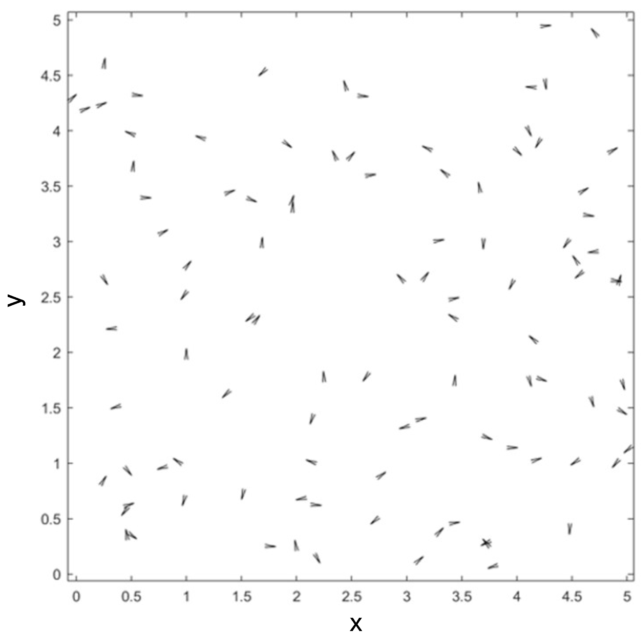
Generation and initialization of UAVs. UAVs were generated at random locations within a square area with a side length of 10 m. The UAVs were initialized with the entropy metric and initialized with the entropy metric. Initial speeds were assigned to these UAVs, aiming to ensure that the clustering algorithm does not fail due to zero initial value while exploring whether a chaotic UAV clustering system can maintain motion consistency. Therefore, the generated UAVs have the following parameters: initial position, velocity, and communication range. The generation of the UAV cluster is shown in Figure 2, where the horizontal and vertical coordinates are equally scaled to the actual units.

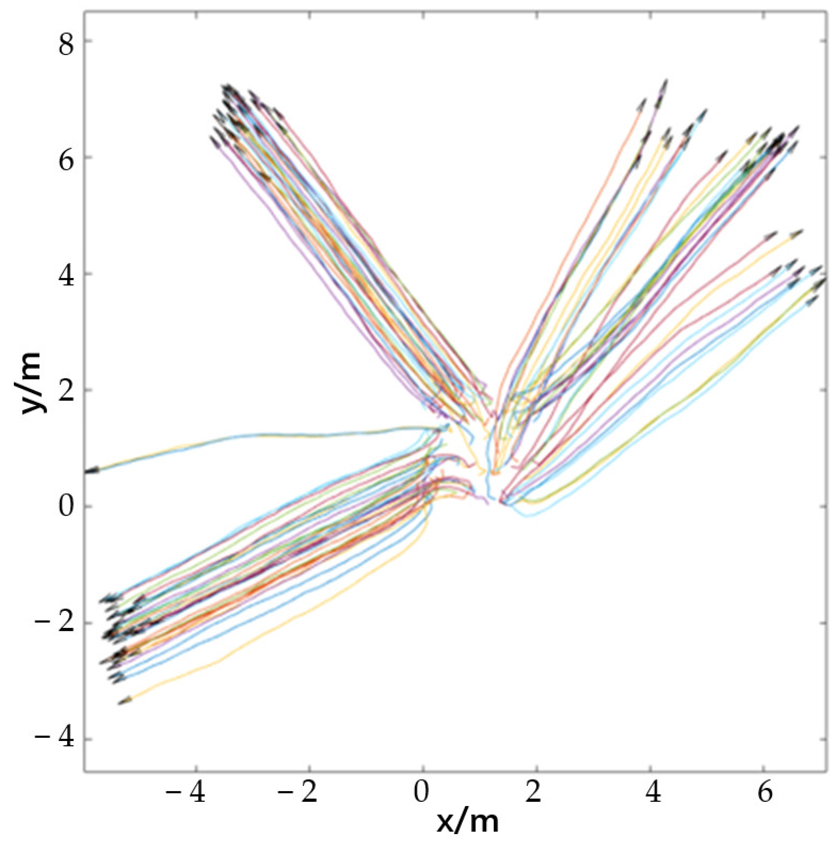
Validation of the clustering algorithm before improvement. To simulate a real communication-constrained environment, the UAV’s communication range was limited, so that it could only sense other UAVs within a small range around it, but not all other UAVs on the map. To validate the algorithm’s effect on cluster stability, the external interference was set as a large random noise, which was used to simulate the effect of the complex flight environment on the cluster. One hundred sets of repeated experiments were conducted, with 50 iterations of the algorithm for each set of experiments. Statistical data found that clusters were clearly formed in 86 of the 100 repetitive experiments, with 69 cases showing cluster dispersion after iterations under strong interference, as shown in Figure 3, in which the horizontal and vertical coordinates are scaled equally to the actual units. The different colors in the figure represent the flight paths of different UAVs. The data also revealed that most of the initialized UAV swarms formed distinct clusters after the 15th to 20th iterations.

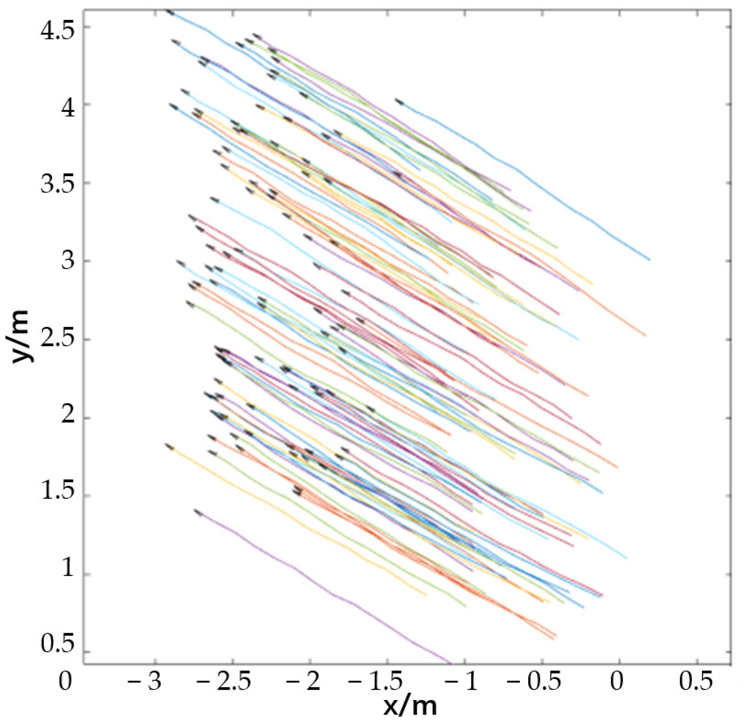
Improved algorithm validation. In this experimental phase, UAVs calculate and exchange entropy metric adaptation values during the algorithm iteration, while the rest of the parameter settings are the same as in the previous step of the experiment. The same 100 sets of repetitive experiments were conducted, and 50 algorithm iterations were performed for each set of experiments. Statistical data revealed that all 100 groups of experiments formed stable clusters, and the clusters could be kept stable after highly noisy algorithm iterations, as shown in Figure 4, where the horizontal and vertical coordinates are scaled equally to the actual units. The different colors in the figure represent the flight paths of different UAVs. Most of the experiments in this part formed obvious clusters after the 10th to 15th iterations. It can be seen that the algorithm introducing the population entropy metric improves the consistency of the cluster motion significantly, and the convergence speed of the cluster motion is improved by about 30%.

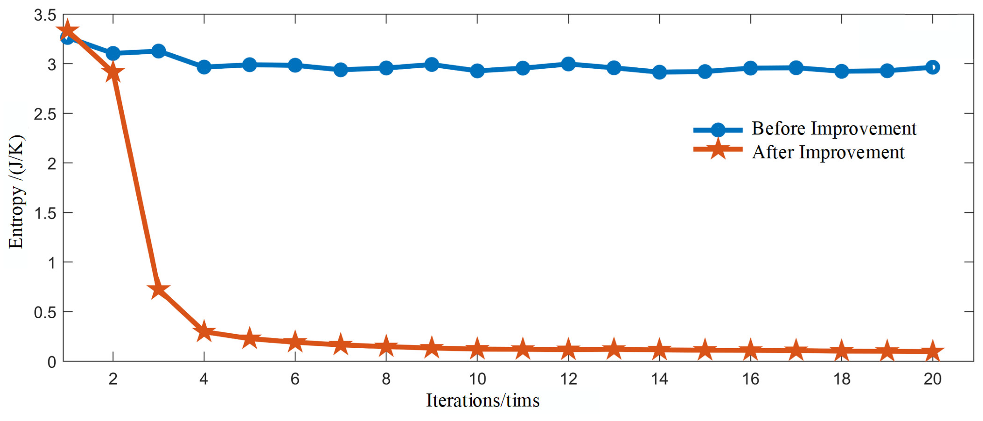
Through the above two parts of the comparison test, it can be seen that the randomly generated UAV swarms generally enter a stable state after 20 iterations. Therefore, the entropy value variance of the UAV samples in the first 20 iterations of the two parts of the experiment is counted separately, and a line graph is plotted, as shown in Figure 5.

Figure 5 demonstrates decreasing entropy variance trends in both experiments, i.e., the algorithm before and after the improvement can cause the randomly generated UAVs to form clusters. However, the sample entropy variance calculated using the pre-improvement algorithm does not have a tendency to converge to 0 after 20 iterations, i.e., the UAV clusters diffuse in the iterative process of high noise, and the entropy variance fluctuates up and down under the influence of noise. The entropy variance of the samples calculated by the improved algorithm shows a tendency to converge to 0 after 20 iterations, i.e., the UAV cluster can remain stable in the iterative process of high noise, and the entropy variance continues to show a decreasing trend under the influence of noise.

Through the comparison experiment, it can be seen that the improvement of the algorithm has significantly enhanced the stability of the multi-UAV cluster under restricted environments. Additionally, the number of iterations of the algorithm required for cluster formation is reduced, and the system convergence speed is faster.

3.2. Physical Simulation Experiment

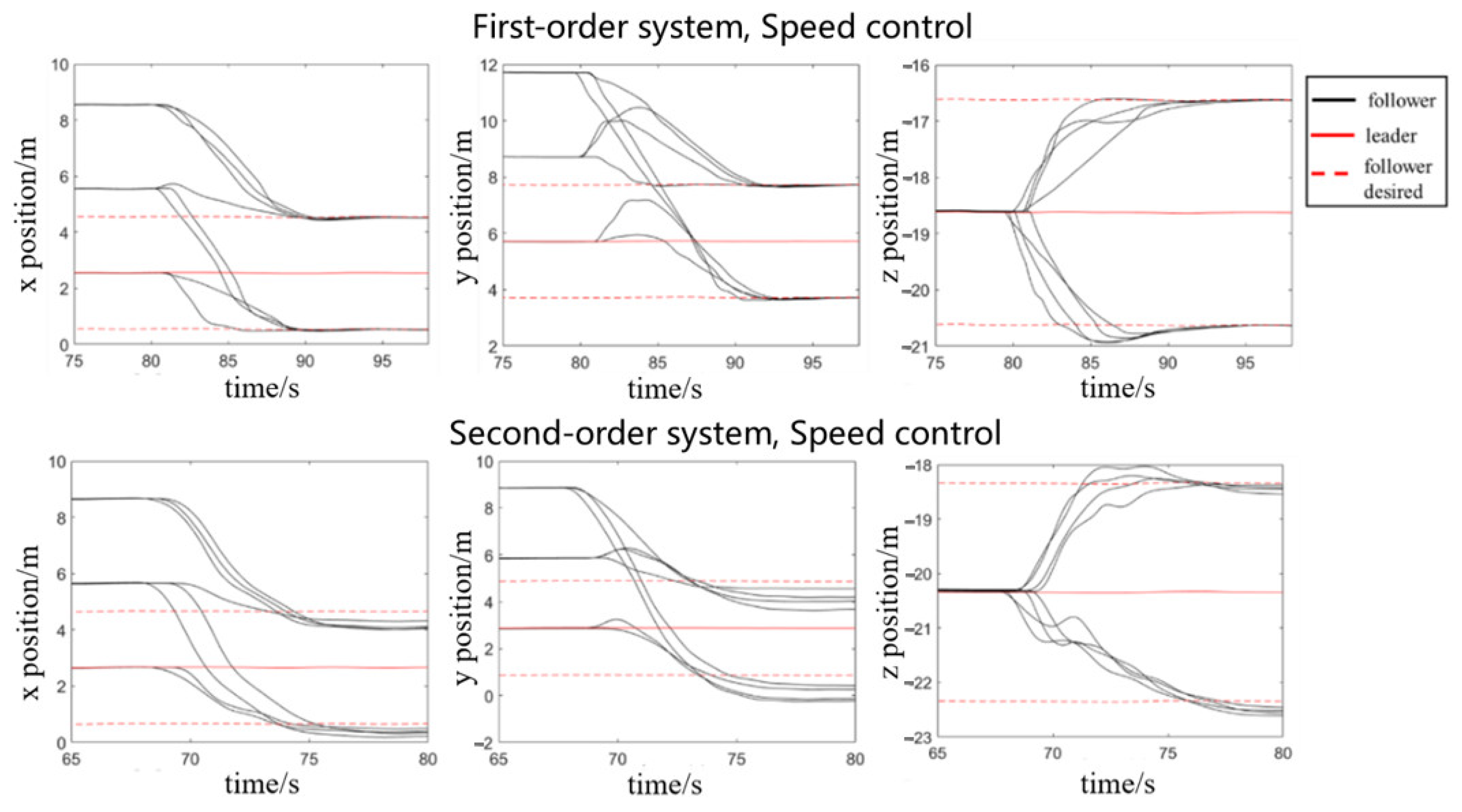
The experiments in the first part initially verified the feasibility and superiority of the improved algorithm, but the simplified 2D UAV model only accounts for two-dimensional motion, which lacks many physically necessary parameters compared to real UAVs. Therefore, in order to prove that the improved algorithm can be applied to a real UAV cluster system, this paper builds a quadrotor UAV model and a complex flight map in the Gazebo physical simulation environment, carrying out UAV cluster physical simulation experiments. In terms of UAV control mode selection during the experiment, a data comparison between velocity control and acceleration control is carried out. As shown in Figure 6, compared with acceleration control, velocity control exhibits higher response speed and a smaller steady-state error; therefore, velocity control UAV flight was used during the experiment.

In the experiments in Section 3.1, UAV-constrained communication under real flight conditions is simulated by limiting the UAV’s perceived range, while external interference is achieved by superimposing random noise on the speed. In the physical simulation experiments, complex flight maps are constructed to represent external interference, characterized by numerous large obstacles, as well as significant wind resistance. Formation obstacle avoidance flight experiments were conducted for two groups of UAV swarms, before and after the algorithm improvement, respectively, as shown in Figure 7.

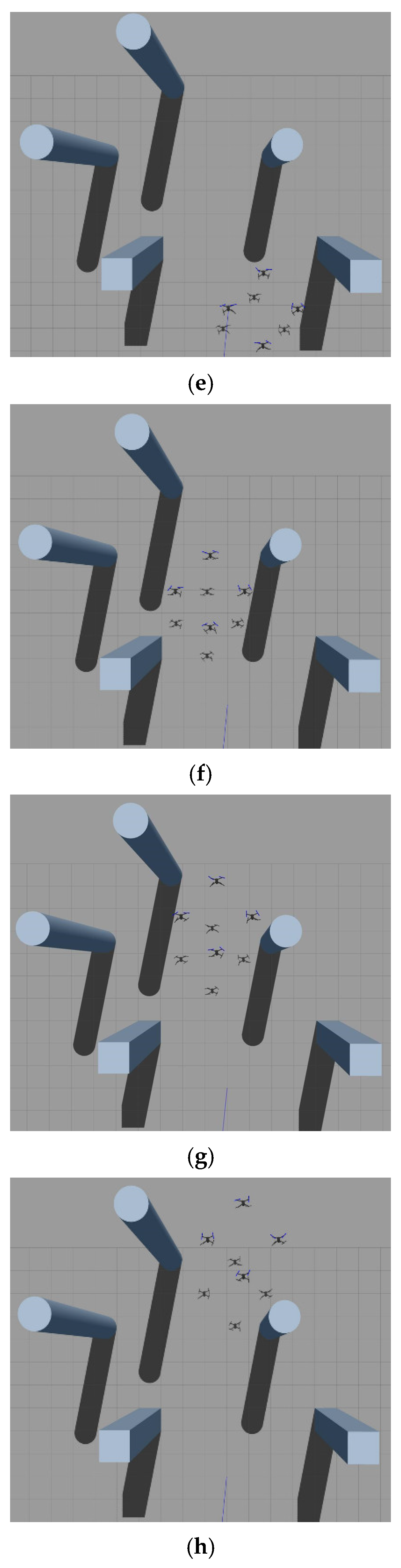
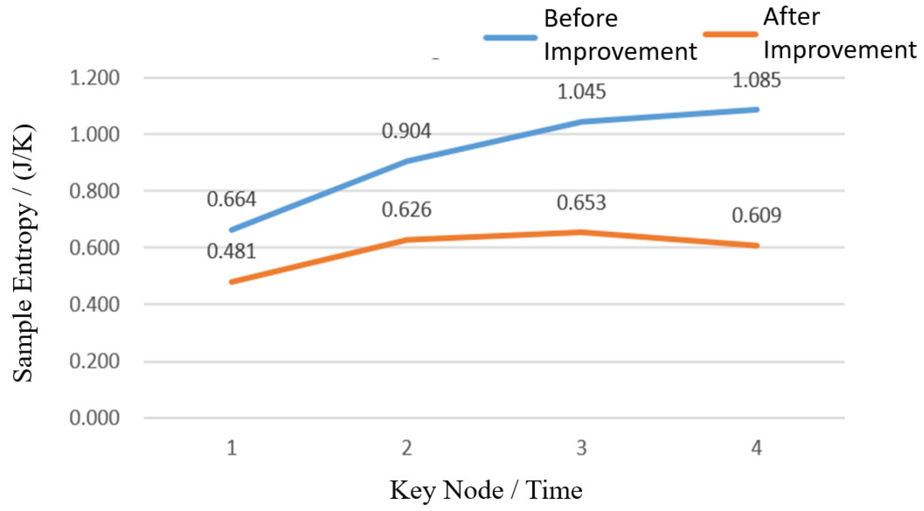
Figure 7 shows the algorithm improvement comparison experiments conducted in the Gazebo simulation environment. In the Figure 7, the blue cylinder is a cylindrical obstacle, and the blue rectangular block is a rectangular obstacle. The shaded part is the shadow of the obstacle and the drone on the ground. Since the system entropy value is calculated iteratively at moments, in order to show the trend of the system entropy value throughout the entire experiment, four time nodes with significant entropy value changes—namely, the starting state, the first obstacle avoidance, the second obstacle avoidance, and the final state after passing through the obstacle—are selected as the key nodes in the experiment. Figure 7a–d shows the four UAV cluster simulation experiments of the pre-improvement algorithm, and Figure 7e–h shows the four UAV cluster simulations of the post-improvement algorithm. A comparison of the two sets of experiments shows that the pre-improved UAV cluster splits significantly when traversing dense obstacles, and the motion consistency is reduced, while the improved UAV cluster still maintains cluster convergence after traversing dense obstacles, and the cluster motion consistency is improved significantly. The individual entropy values and system entropy values of UAV clusters at four key nodes in the two experiments are plotted as line graphs, as shown in Figure 8 and Figure 9.

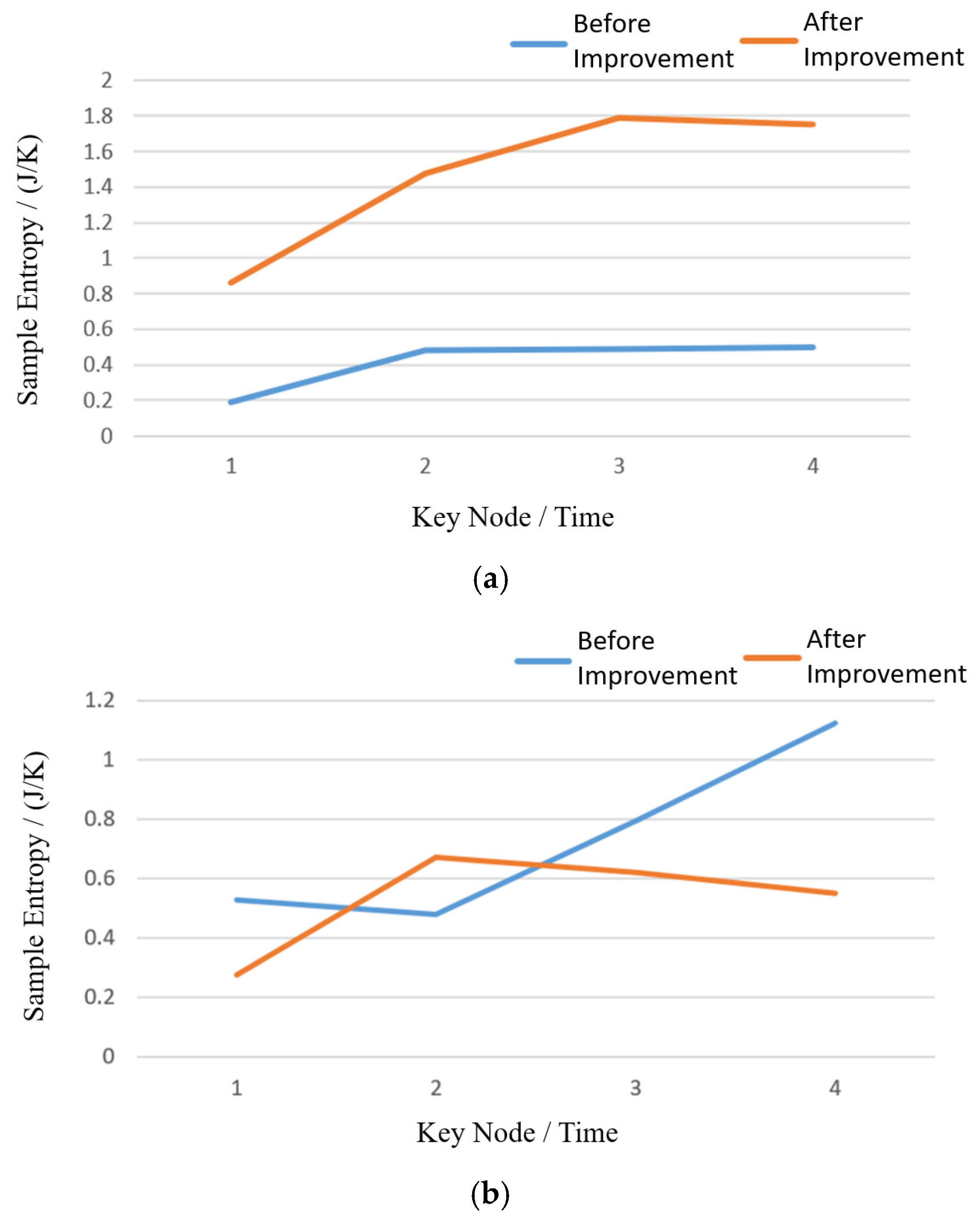
In Figure (a), it is evident that the entropy values of the algorithm before improvement is significantly higher than after improvement. In Figure (b), the entropy values of the improved algorithm is relatively high only at node 2, while it remains low at all other nodes. In Figure (c), although there is little difference in entropy between the original and improved algorithms for the first three nodes, a noticeable gap emerges from node 4 onward. Figure (d) exhibits a trend similar to Figure (a), where the entropy values of the improved algorithm is significantly lower. By comparing the data in Figure 8, it can be seen that, except for the first aircraft, the individual entropy values of UAVs after the algorithm improvement is generally lower than those before the improvement, and all of them can be adaptively adjusted to the state of entropy decreasing after the entropy increase, i.e., each aircraft can converge to the stable state of self-adaptive adjustment in the complex flight environment.

Figure 9 reveals an overall entropy increase at four key nodes in both experiments. However, the overall entropy value of the system in the experiment before improvement has increased, indicating that the stability of the UAV cluster system gradually decreases. The average value of the system entropy value is 0.925, and the fluctuation range of the entropy value in the experimental process is within 63.4%. In contrast, the system entropy value of the system in the experiments after improvement shows a rising trend in the process of obstacle avoidance; however, the overall level of the system entropy value is significantly lower than that of the pre-improvement period, and it shows a decreasing trend after the end of the obstacle avoidance period. The stability level of the UAV cluster system in the flight process is improved overall compared with the pre-improvement level, and it is able to adaptively adjust according to the complex changes in flight constraints to maintain the consistency of the UAV cluster motion. The average value of the system entropy value is 0.587, and the fluctuation range of the entropy value is within 41.6%, i.e., the consistency of the UAV cluster motion, with the introduction of the group entropy metric, is improved by 21.8%.

The comparison of the two sets of experiments shows that when UAVs are clustered using the pre-improved algorithm, they adopt a scattered bypass to pass through obstacles. Due to the lack of inter-aircraft gravitational force when encountering obstacles, multiple avoidance attempts often result in individual UAVs losing their communication due to the spreading of distances, which leads to the dispersion of the clusters. When UAVs are clustered using the improved algorithm, the entropy metric is used to make up for the shortcomings caused by the lack of inter-machine gravity and is able to maintain stable clusters even after multiple obstacle avoidance attempts, which improves the consistency of the UAV’s clustering motion.

In the previous experiments, random noises in nature are modeled by simulation software, such as the positioning error of GPS and the change in wind resistance of flight. These disturbances are difficult to simulate accurately, so it is necessary to conduct flight experiments with physical prototypes to verify the effectiveness of the cluster model and algorithm proposed in this paper.

The multi-UAV cluster flight experiment process is complex, dangerous, and requires a certain amount of experimental equipment and manpower investment. Autonomous UAVs require real-time monitoring by the pilot to ensure that manual operation can be taken over at any time to prevent the system from going out of control and causing safety problems. Fully autonomous UAV cluster flights require a ground station to collect experimental data, calculate flight data in real time, and forward the speed and position information of the UAVs; thus, there is also a certain requirement for communication capacity. Considering the hardware and software equipment in the laboratory, the fully autonomous cluster flight experiment of three UAVs is designed. Three constitutes the minimum cluster lattice size, as fewer aircraft cannot adequately demonstrate that it is not enough to react to the interaction between the UAVs in the cluster, making it difficult to visualize the effect of the cluster algorithm.

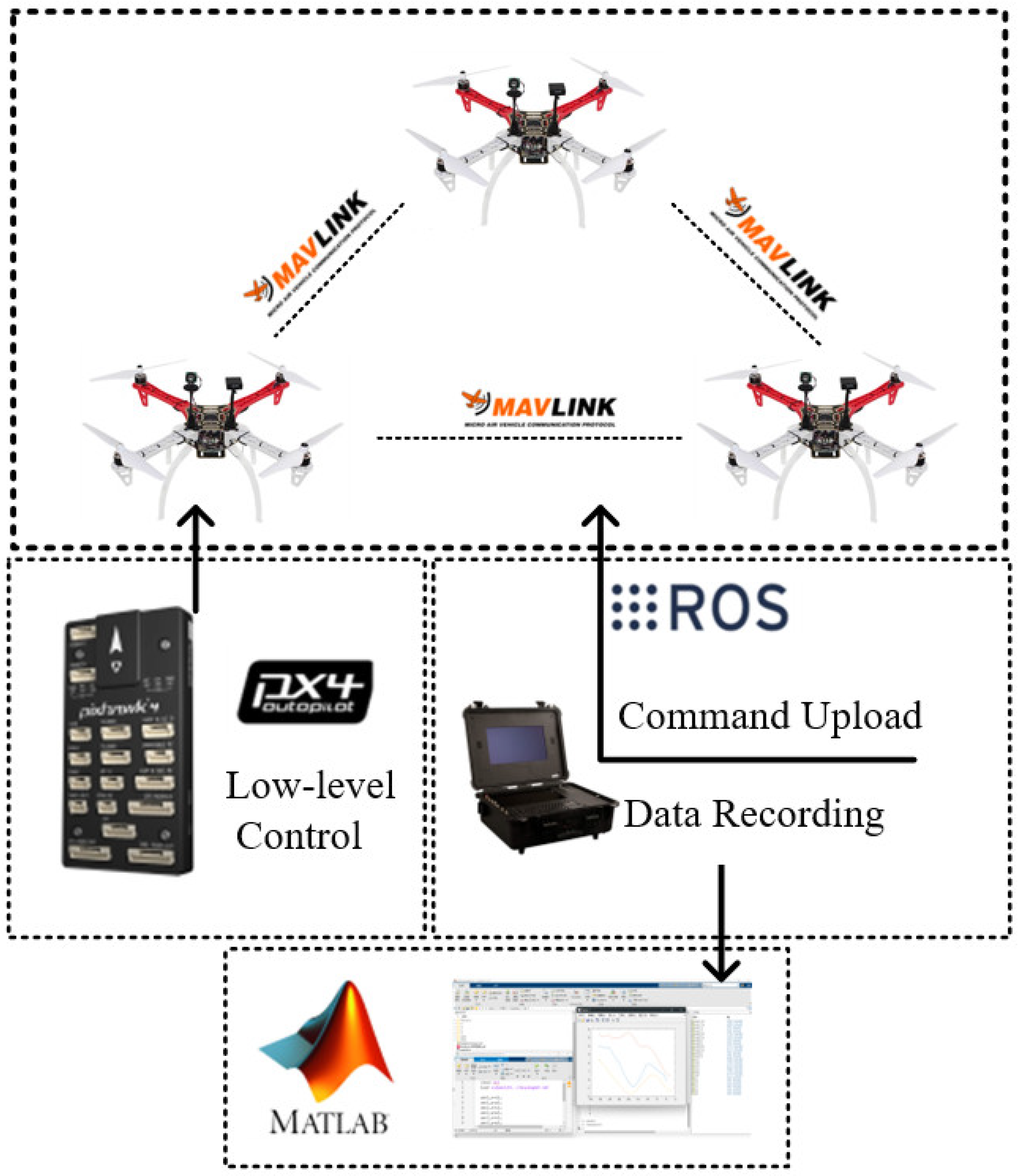
In this paper, we construct a rotary-wing UAV cluster physical prototype test platform to verify the algorithm proposed in Chapter IV. Among them, a UAV hardware system based on self-development is designed with PIXHAWK (Holybro, Shenzhen, China) flight control as the core. The communication protocol was developed on MAVLINK (PX4 Development Team, Open Source), which functions to enable communication between the UAV and the ground station. The interactive software used QGC, which facilitated the exchange of information and task release. Data processing was carried out on the MATLAB graphical interface to enable the analysis of the logged cluster data. Figure 9 shows the hardware platform block diagram.

In terms of hardware selection for the quadcopter UAV, the UAV adopts the PIXHAWK open-source flight control, which offers excellent performance, high expandability, and facilitates secondary development. The quadcopter’s spatial position, velocity, attitude, and collective rotational speed are controlled in a closed loop by the PIXHAWK flight controller, eliminating the need to calculate the tedious flight control parameters in the experimental process. The DJI F450 is used for the frame, which has the advantages of a lightweight structure and strong load capacity, providing 15 min of continuous flight time on full charge, ensuring experimental continuity. The GPS positioning module is equipped to ensure that the UAVs have a high positioning capability, and GPS positioning errors originate inherently from the module, so there is no need to add extra calculations.

In the experiment, each UAV needs to send and receive speed and position information within its interaction range and calculate its own speed in the next cycle of the algorithm; thus, it is necessary to choose the appropriate onboard computer and communication equipment. The NVIDIA Jetson TX2 onboard computer handles data collection and computation and transmits the speed of the next cycle to the PIXHAWK flight control board. It has the advantages of being lightweight and having strong computational ability, which can meet the needs of this experiment. The P900 communication module was selected, which supports the characteristics of a central node connecting multiple sub-nodes, with a maximum transmission distance of 20 km, operating at an 800 MHz frequency with 1.4 MHz bandwidth, which can fulfill the communication requirements of this experiment.

The experimental UAV and its hardware architecture are depicted in Figure 10.

The UAV used in the experiment and its hardware structure are shown in Figure 11, where Figure 11a is the overall appearance of the drone and Figure 11b is a block diagram of the drone’s core hardware components.

3.2.1. Experimental Design of Physical Prototype

The program design of the physical prototype experiment mainly focuses on the decision-making procedure of the UAV, including three modules: information interaction code, flight strategy code, and underlying control code. The information interaction code is used to transfer speed and position information between UAVs and transmit it to the TX2 onboard computer. The flight strategy code is used to determine the desired flight speed based on the position speed of the local UAV and the position speeds of its neighbors at the current moment and transmit it to the PIXHAWK flight control board. The underlying control code is used to manage the flight of the UAV.

In terms of quadcopter UAV communication, there are two main communication protocols in the UAV control system. One is the communication protocol between multiple nodes with MAVLINK as the core, which realizes the sending and receiving of the UAV’s position information. The other is the communication protocol between each processing program in the flight control system, which is based on ORB information. The motion consistency entropy metric theory designed in this paper is mainly calculated based on the velocity and position samples of each UAV in the cluster; therefore, it is necessary to customize the MAVLINK message to facilitate the calculation and release of the velocity of each UAV during the cluster flight.

The main steps of the physical prototype experiment are as follows:

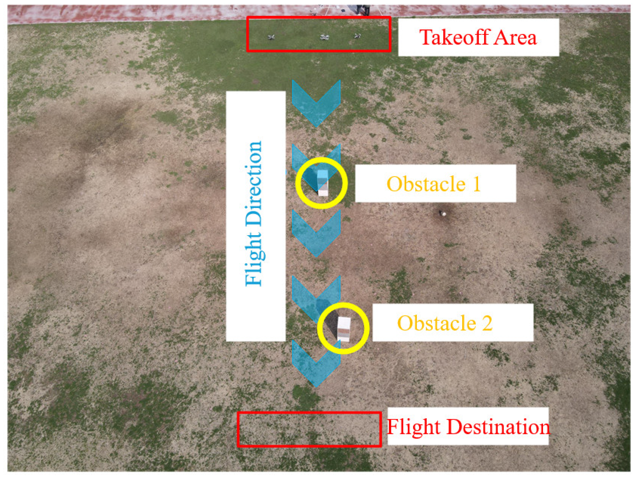
(1) Port the relevant parameter files for UAV control in the GAZEBO simulation program to the onboard computer, and set the takeoff point and target point for the UAV according to the actual flight position, so that it can fly autonomously toward the target point after takeoff. This ensures that the UAV cluster will definitely cross the obstacle area during flight, allowing for an analysis of the consistency of the motion of the UAV cluster flight. The scene layout of the experiment is shown in Figure 12:

Considering the safety of the experiment, it is necessary to impose certain restrictions on the aircraft before takeoff: maximum speed (2 m/s), altitude limit (3 m), and set up an electronic fence around the test site, so that the UAV will land automatically when it flies out of the fence.

(2) Power on the UAVs and wait for the PIXHAWK flight control board to search for GPS positioning information. All three UAVs automatically take off after obtaining GPS information, change formation to cluster lattice automatically, and fly toward the target point, crossing the pre-set obstacles on the way.

(3) All three UAVs landed automatically when they flew to the vicinity of the target point, and the flight data were exported and analyzed.

3.2.2. Experimental Results and Analysis of Physical Prototype

This section presents physical prototype experiment results and analyzes the UAV flight trajectory, speed changes, entropy changes, and flight altitude changes.

(1) Cluster flight process. The whole process of the experiment is shown in Figure 13. In Figure 13, the red circle represents the three UAV used in the experiment, the yellow circle represents the rectangular obstacle, and the yellow dashed line represents the virtual connection between each UAV, which is used to display the positional relationship between the UAV clusters. Before takeoff, the starting positions of all UAV are placed on the same straight line, as shown in Figure 11a. After takeoff, the UAV swarm forms a triangular cluster structure, as shown in Figure 11b. Figure 11c,d show the situation of the UAV cluster in the first and second obstacle avoidance situations.

(2) Flight trajectory analysis. The trajectory route of each UAV in the experiment is shown in Figure 14:

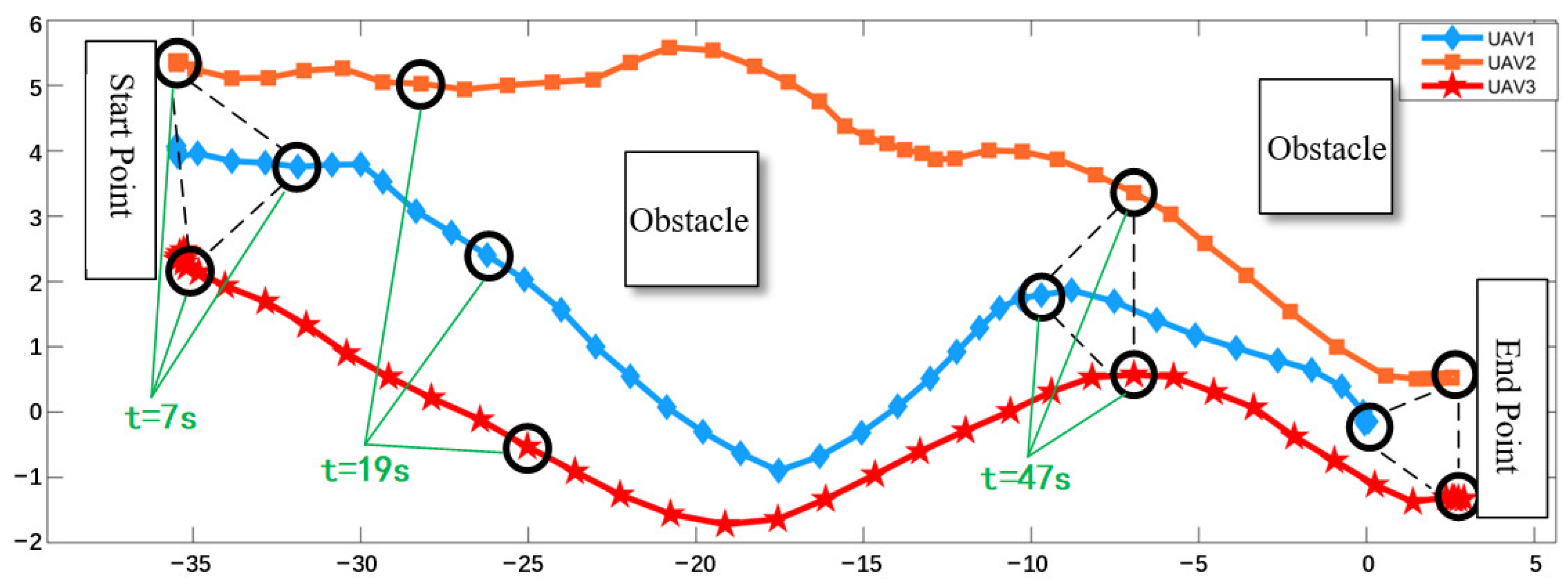
The blue diamond-shaped line in Figure 14 represents the flight trajectory of UAV #1, or UAV1; the orange square line represents the flight trajectory of UAV #2, or UAV2; and the red star-shaped line represents the flight trajectory of UAV #3, or UAV3. For easier comparison, the time points corresponding to the graph are labeled in the figure.

Figure 13a shows the pre-flight linear UAV arrangement. The three UAVs were powered on and automatically searched for GPS positioning information; all of them searched, then automatically took off and entered the autonomous swarm mode. At t = 7 s post-takeoff, the UAVs formed an equilateral triangular formation, and Figure 13b shows the cluster state of the three UAVs, while their relative positions are shown in Figure 13b at t = 7 s. At about 19 s after takeoff, the three UAVs perform the first obstacle avoidance. Figure 14 shows the three UAVs executing this maneuver, and their relative positions are shown at t = 19 s in Figure 13c. At about 47 s after takeoff, the three UAVs perform the second obstacle avoidance. Figure 13d shows the three UAVs executing this avoidance, and their relative positions are shown at t = 47 s in Figure 14. At about 1 min after takeoff, the three UAVs flew to the vicinity of the target point and landed after automatically hovering to adjust their positions. Figure 13e shows the landing state of the three UAVs, and their relative positions are shown on the rightmost side in Figure 14.

At about 47 s after takeoff, i.e., when the UAV cluster flies to the vicinity of the second obstacle, it can be observed that the three UAVs form an approximate equilateral triangle cluster configuration again, which proves the validity of the motion consistency algorithm based on the entropy metric. In the cluster configuration formed at about 7 s after takeoff, UAV1 is in front (due south) of the remaining two, while in the cluster configuration formed for the second time, UAV2 is behind (due north) of the remaining two. This phenomenon occurs because of UAV1’s proximity to the obstacle, thus generating a larger collision avoidance velocity component between the real UAV and the virtual UAV, which results in a larger deviation from the original flight trajectory and a relatively longer flight trajectory path. In order to ensure the safety of the experiment, the speed of the UAV has been limited to less than 2 m/s prior to the experiment, so that UAV1 will be at the rear of the remaining two UAVs during the second obstacle avoidance.

(3) Speed change analysis. The velocity change in the three UAVs in the cluster is shown in Figure 15:

The blue hexagonal line in Figure 14 represents the change in speed over time for UAV1; the orange square line denotes the change in speed over time for UAV 2, UAV 2; and the red star-shaped line represents the change in speed over time for UAV 3, UAV 3. Analysis reveals all UAVs exhibited a velocity reduction at t = 7 s post-takeoff. Comparative analysis reveals that about 7 s after takeoff is the time when the UAVs first form a clustered configuration, indicating that the deceleration of the UAVs implies that the position adjustment is complete, and the traversing flights begin. UAV1’s velocity decreased sharply at t = 19 s, which is analyzed by comparison as the first obstacle avoidance moment. This is also the reason why the position of UAV1 changes relative to the other two UAVs at the end of the test. UAV2 experienced a velocity reduction at t = 25 s, and the comparative analysis shows that when UAV2 is flying between the two obstacles, it is subjected to the collision avoidance component from the virtual UAVs at the edges of both obstacles at the same time. These opposing collision avoidance vectors partially negate, constraining UAV2’s velocity. During t = 25–47 s, converging velocities indicate that the consistency of the cluster motion is improving and the entropy of the cluster motion is decreasing, which satisfies the algorithm designed in Chapter IV. At about 47 s after takeoff, the speeds are once again different, and the comparative analysis concludes that the cluster is performing the second obstacle avoidance. The three UAVs flew to the end of the vicinity for a short position adjustment, and the speeds gradually converged. Finally, the UAVs landed automatically, and all the speeds gradually decreased to zero.

(4) Entropy value change analysis. The entropy value change in the three UAVs in the cluster is shown in Figure 16:

In Figure 16, the blue hexagonal line represents UAV1, i.e., the change in entropy value of UAV1 over time; the orange square line represents UAV2, i.e., the change in entropy value of UAV2 over time; and the red star-shaped line represents UAV3, i.e., the change in entropy value of UAV3 over time. Data analysis of the above figure shows that the entropy values of UAV2 and UAV3 increase about 19 s after takeoff. A comparative analysis reveals that it is the time of UAV1’s first obstacle avoidance. Due to the decrease in UAV1’s flight speed, the speed differentials with UAV2/UAV3 increased; therefore, the entropy values of UAV2 and UAV3 increased. About 25 s after takeoff, the entropy values of UAV1 and UAV3 increase, and the comparative analysis reveals that UAV2 is in the middle of two obstacles. The speed of UAV2 is limited by two obstacles at the same time, causing it to decrease, and the difference between its speed and that of UAV1 and UAV3 increases, so the entropy value of UAV1 and UAV3 increases. During the period from about 25 s to 47 s after takeoff, the entropy values of all three UAVs show a decreasing trend, indicating that system entropy adaptively decreased through algorithmic iteration. The entropy value increases again at about 47 s after takeoff, and the comparative analysis shows that the cluster is performing the second obstacle avoidance. At this time, UAV1 flies to the backside of UAV2 and UAV3, and the difference in speed causes the entropy value of the two UAVs to increase. Then, the entropy value of the three UAVs continues to decrease until the end of the flight. A comprehensive comparison reveals that the entropy value of the UAV cluster decreases after two obstacle avoidance, verifying the effectiveness of the algorithm designed in Chapter IV.

(5) Flight altitude change analysis. The flight altitude changes in each UAV in the cluster are shown in Figure 17:

The blue hexagonal line in Figure 17 represents the change in height over time for UAV number one, i.e., UAV1; the orange square line represents the change in height over time for UAV number two, i.e., UAV2; and the red star-shaped line represents the change in height over time for UAV number three, i.e., UAV3. For experimental safety considerations, the maximum height of the UAVs was limited to 3 m prior to the experiment. The three UAVs reached their maximum altitude at about 5 s after takeoff and then maintained altitude within ±0.2 m of 3 m during flight. UAV2 and UAV3 landed at 51 s after takeoff, while UAV1 landed at 55 s after takeoff. Comparing the flight trajectory diagrams, UAV1 conducted positional adjustments during t = 51–55 s.

The physical prototype experiment shows that the UAV self-organized cluster model designed in this paper can be deployed in the cluster system, and the UAV motion consistency algorithm based on the entropy metric designed in this paper can effectively enable the cluster to converge quickly. The UAV cluster is able to react quickly to external obstacles during flight, and at the same time, it can take into account the collision avoidance between UAVs within the cluster, thus enhancing the UAV cluster motion consistency under multi-constraint conditions.

In the research of this paper, the adaptive parameters are mainly reflected in the calculation of the influence weights in the velocity alignment component. We achieve the adaptive adjustment of the UAV velocity calculation by transforming the fitness value into the influence weights of each UAV in the velocity alignment component. Judging from the experimental results, whether in the algorithm verification experiment or the physical simulation experiment, the improved algorithm with the introduction of swarm entropy measurement performs remarkably. In the algorithm verification experiment, this improved algorithm increases the convergence speed of the UAV swarm by about 30% and is more stable under high noise, while the swarm of the original algorithm is prone to dispersion. In the physical simulation experiment, the motion consistency of the swarm is significantly improved, and the fluctuation range of the system entropy value is reduced by 21.8%. This indicates that the improved algorithm can effectively guide the UAV swarm to evolve toward a better state. From a theoretical analysis perspective, the definition and calculation of swarm entropy show that the algorithm iteration optimizes the system in the direction of entropy reduction. Reasonable influence weights in velocity alignment can reduce the velocity differences among UAVs, decrease the swarm entropy value, and make the system more orderly and stable. This implies the convergence of the algorithm and, to a certain extent, shows that the algorithm may achieve a local optimal solution. However, due to the complexity and uncertainty of the actual environment, as well as the limitations of the algorithm itself, we are currently unable to strictly prove theoretically that it can achieve a globally optimal solution. In the subsequent research, we will conduct in-depth relevant theoretical analysis and supplement this part of the content.

4. Conclusions

Traditional UAV swarm models often overlook the constraints imposed by real-world flight environments. However, precise modeling is a prerequisite for ensuring stable UAV flights. To address this issue, we introduce the concept of self-organization into UAV swarm control and establish a self-organizing model based on velocity and position. Meanwhile, to mitigate issues such as oscillation and loss of control that arise during swarm motion, we propose an adaptive interaction-based entropy metric theory. This theory formulates an entropy-based metric function to evaluate the stability of swarm coordination, thereby enabling adaptive regulation of UAV motion consistency in complex environments. Furthermore, we construct a realistic quadrotor UAV model in a simulation platform. By analyzing real UAV flight data decoded from Pixhawk flight control source code, we validate the feasibility of our swarm model in real-world flight scenarios. Finally, we conduct an obstacle-crossing experiment with three UAVs, demonstrating that the proposed entropy metric theory effectively enhances the motion consistency of UAV swarms.

5. Future Studies

Looking to the future, with the development of technology and the expansion of application requirements, more tasks require UAVs to fly in swarms in complex environments. Follow-up research will focus on how to enable UAV swarms to maintain flexible and stable motion like natural organisms under various constraints. On the one hand, in-depth research will be carried out on the motion characteristics of UAV swarms under more complex interference factors, and the model will be improved to adapt to more actual scenarios. On the other hand, efforts will be made to improve the performance of UAV swarms in large-scale and complex task scenarios, promoting the wide application of UAV swarm technology in more fields.