Fuzzy Amplitudes and Kernels in Fractional Brownian Motion: Theoretical Foundations

Abstract

In this study, we present a novel mathematical framework for pricing financial derivates and modelling asset behaviour by bringing together fractional Brownian motion (fBm), fuzzy logic, and jump processes, all aligned with no-arbitrage principle. In particular, our mathematical developments include fBm defined through Mandelbrot-Van Ness kernels, and advanced mathematical tools such Molchan martingale and BDG inequalities ensuring rigorous theoretical validity. We bring together these different concepts to model uncertainties like sudden market shocks and investor sentiment, providing a fresh perspective in financial mathematics and derivatives pricing. By using fuzzy logic, we incorporate subject factors such as market optimism or pessimism, adjusting volatility dynamically according to the current market environment. Fractal mathematics with the Hurst exponent close to zero reflecting rough market conditions and fuzzy set theory are combined with jumps, representing sudden market changes to capture more realistic asset price movements. We also bridge the gap between complex stochastic equations and solvable differential equations using tools like Feynman-Kac approach and Girsanov transformation. We present simulations illustrating plausible scenarios ranging from pessimistic to optimistic to demonstrate how this model can behave in practice, highlighting potential advantages over classical models like the Merton jump diffusion and Black-Scholes. Overall, our proposed model represents an advancement in mathematical finance by integrating fractional stochastic processes with fuzzy set theory, thus revealing new perspectives on derivative pricing and risk-free valuation in uncertain environments.

1. Introduction

We will now describe the dynamics of a particle, considering the uncertainties involved. The underlying stochastic process is modelled by a fractional Brownian motion (fBm), known for its long-range dependence and self-similarity, which makes it suitable for financial modelling. Fractional Brownian motion is traditionally employed in financial modelling due to its ability to represent memory effects through the Hurst exponent with values significantly influencing the roughness or smoothness of volatility [1].

The model involves fuzzy processes, denoted by x_ε(t), which are functions that map the time parameter t to a set of possible values in R with certain degrees of membership that quantify uncertainty or ambiguity inherent to market expectations. Unlike traditional models that typically incorporate either fBm or fuzzy logic individually, our approach combines both techniques to offer a more robust and realistic characterisation of market uncertainty.

We consider a stochastic differential equation (SDE) that includes a linear drift coefficient μ and a volatility coefficient σ, both initially assumed constant. To find the closed explicit fuzzy solution for μ ≥ 0, the system of equations is solved to obtain the fuzzy solutions $X_{\epsilon }^l\left(t\right)$ and $X_{\epsilon }^u\left(t\right)$ for the lower and upper bounds, respectively.

Similarly, the solution is derived for μ < 0 by obtaining the fuzzy solutions $X_{\epsilon }^l\left(t\right)$ and $X_{\epsilon }^u\left(t\right)$ for the lower and upper bounds, respectively. We used existing results from [2,3] to extend the unique solution to the fuzzy stochastic fractional differential equation (FSFDE) for μ ≥ 0. According to these results, which provided certain regularity conditions such as Lipschitz continuity with constant L of the function a, continuity of the function b, and σ which is locally Lipschitz continuous, then there exist constants K and p such that ||σ(x)|| ≤ K(1 + ||x||^P) for all x. Then, for any initial condition X(0) = x(0) with probability 1, there exists a unique solution to the FSFDE in the form:

$$dX\left(t\right)=\left[aX\right(t)+b]dt+\sigma \left(X\right(t\left)\right)dW\left(t\right),$$

where W(t) is a standard d-dimensional Wiener process.

The key idea is to show that when h > ½, the matrix-valued function a, the vector-valued function b, and the matrix-valued function σ satisfy certain regularity conditions that enable us to apply standard techniques from the theory of stochastic differential equations to prove the existence and uniqueness of a solution to the FSFDE. In particular, the Lipschitz continuity condition on ‘a’ ensures the local boundedness of the solution, while the local Lipschitz continuity condition on σ ensures that the solution is almost surely continuous. The continuity condition on ‘b’ ensures that the drift term is well-defined and continuous.

In relation to the recent studies such as [4,5], the current paper is more focused on the theoretical development of the model. Ref. [5] builds directly on Merton’s jump-diffusion model, introducing fuzziness to parameters such as the stock prices, risk-free rate, and jump intensities. It applies a bisection search algorithm to compute the belief degree of option prices and empirically validate the model using NIFTY 50 and Nikkei 225 data. In contrast, ref. [4] employs a mixed fBm framework, emphasising the modelling of long memory and jump behaviour with fuzziness applied to a broad set of parameters.

The current work delves deeply into theoretical extensions, introducing a custom PDE with exponential and hyperbolic functions to handle negative drift and extending Feynman-Kac bridging techniques. The current work also contributes novel mathematical structures by formalising FFBM for H < ½, applying Girsanov’s theorem in a fuzzy context, incorporating Molchan martingale techniques for bounding the supremum of fuzzy fBm.

Moreover, we provide explicit numerical simulations demonstrating clear enhancements over traditional approaches such as Merton’s jump-diffusion model, highlighting how our hybrid fuzzy-fractional methodology yields superior flexibility and adaptability under realistic market conditions. These illustrative simulations substantiate our theoretical claims by clearly showing that the combined fuzzy-fractional model improves uncertainty modelling. In summary, our approach not only offers novel theoretical extensions in stochastic calculus but also demonstrates practical advantages for modelling financial derivatives through explicitly accounting for both fuzziness and fractional memory.

2. Applications

We start with the typical partial differential equation used in mathematical finance.

$$X\left(t\right)=X_0+{\int }_0^t\mu X\left(s\right)ds+{\int }_0^t\sigma X\left(s\right)d{B}_H\left(s\right), X_0=X\left(0\right),$$

where X(t) is the value of the financial quantity at time t, X(0) is the initial value of X at time 0, μ and σ are constants representing the drift and volatility of X, respectively, and B_H(s) is the fractional Brownian motion (fBm) process which has long-range dependence and self-similarity properties. We already covered why the fBm process is used in financial modelling. In summary, it can capture the long-term dependencies in financial data, which are not always captured by traditional Brownian motion processes. This makes it suitable for modelling financial quantities that exhibit long-term trends or memory effects. Unlike crisp partial differential equation, the equation involving uncertainties is modelled using fuzzy processes. In the case of linear coefficients, an explicit solution can be obtained. The fractional fuzzy stochastic differential equation (FFSDE) satisfies the assumptions of Yamada-Watanabe-Kunita theorem and the Kushner-Stratanovich equation. The Yamada-Watanabe-Kunita theorem provides conditions for the existence and uniqueness of solutions to certain types of SDEs [6]. Statement of the Theorem—consider the following stochastic differential equation:

$$dXt=b\left(Xt\right)dt+\sigma \left(Xt\right)dWt,$$

where:

-

X_t is the stochastic process to be solved.

-

b(X_t) is a drift function that depends on X_t.

-

σ(X_t) is a diffusion function that depends on Xt.

-

W_t is a standard Wiener process (Brownian motion).

The Yamada-Watanabe-Kunita theorem requires the following assumptions to be satisfied:

1. The functions b(X) and σ(X) are globally Lipschitz continuous in X with a Lipschitz constant that is independent of time t. In other words, there exists a constant K such that for all x, y in the state space of X, we have:

$$\begin{array}{c}\left|b\right(x)-b(y\left)\right|\le K|x-y|\\ \left|\sigma \right(x)-\sigma (y\left)\right|\le K|x-y|\end{array}$$

2. The functions b(X) and σ(X) satisfy a linear growth condition. That is, there exist constants M and L such that for all x in the state space of X, we have:

$$\begin{array}{c}\left|b\right(x\left)\right|\le M(1+|x\left|\right)\\ \left|\sigma \right(x\left)\right|\le L(1+|x\left|\right)\end{array}$$

SDE is nondegerate meaning the diffusion(covariance) matrix σσ^T is positive definite everywhere. Under these assumptions, the Yamada-Watanabe-Kunita theorem guarantees the existence and uniqueness of a strong solution to the stochastic differential equation:

$$dX\left(t\right)=bX\left(t\right)dt+\sigma X\left(t\right)dWt.$$

The theorem is essential because it establishes the conditions under which solutions to certain stochastic differential equations exist and are unique. The key idea behind the Yamada-Watanabe-Kunita theorem is to show that the nonlinearity of the drift and diffusion coefficients can be controlled by the Lipschitz and growth conditions, respectively, so that the SDE admits a unique solution. The theorem has been extended to FFSDEs, which are SDEs with fuzzy coefficients. In this context, the theorem provides conditions for the existence and uniqueness of solutions to FFSDEs and has important applications in the modelling of systems with uncertain or imprecise information.

The second important condition is the FFSDE model must satisfy the Kushner-Stratonovich equation [7]. It arises in the context of state estimation problems, where the goal is to estimate the unobservable state of a dynamic system based on noisy measurements. The Kushner-Stratonovich equation applies to a class of SDEs that can be written in the following form:

$$d{X}_t=f\left(X_t\right)d_t+g(X_t, t) d{W}_t,$$

where:

X_t is the unobservable state of the system at time t.

f(X_t, t) is a drift function that describes how the state X_t evolves over time. It depends on both the current state X_t and the time t.

g(X_t, t) is a diffusion function that accounts for the effect of random noise on the system. It also depends on the state X_t and time t.

dW_t represents the increment of a Wiener process (Brownian motion), which represents the random noise or uncertainties in the system.

The main challenge in the theory of filtering is to find an optimal estimate of the state X(t) given the available measurements up to time t. This estimate is usually denoted by $\widehat{x_t}$ and is known as the filter. Solving the Kushner-Stratonovich equation involves finding the filter $\widehat{x_t}$ that minimizes the mean squared error between the true state X(t) and the estimated state $\widehat{x_t}$. The key idea behind the equation is to express the SDE in a form that separates the drift and diffusion terms, so that it can be solved using standard techniques from the theory of stochastic calculus. The Kushner-Stratonovich equation takes the following form:

$$dX\left(t\right)=\left[f\right(X\left(t\right))+1/2g(X\left(t\right)\left)g^{\prime }\right(X\left(t\right)\left)\right]dt+g\left(X\right(t\left)\right)dW\left(t\right),$$

where g′ denotes the derivative of g with respect to its argument. The equation represents an alternative to the Itô formula, which is commonly used to derive solutions to SDEs with linear drift and diffusion coefficients. In contrast to the Itô formula, which involves a stochastic integral with respect to the Wiener process, the Kushner-Stratonovich equation involves a deterministic integral with respect to the derivative of the diffusion coefficient. We have explained two important theorems that were used in this work’s derivations.

The equation we are deriving is a stochastic differential equation (SDE) describing a system with two state variables, $X_l^{\mathsf{\epsilon }a}(t)$ and $X_u^{\mathsf{\epsilon }a}\left(t\right).$ The SDE has a Wiener process W, which represents the random noise in the system. The SDE can be divided into two cases depending on the value of the drift coefficient μ. When μ ≥ 0, the unique solution to the SDE can be obtained using Feynman-Kac Theorem. The solution for $X_l^{\mathsf{\epsilon }a}(t)$ and $X_u^{\mathsf{\epsilon }a}\left(t\right)$ can be expressed in a matrix form. The solution involves exponentials of μt, α, and the Wiener process W. When μ < 0, the unique solution to the SDE can also be obtained using the same theorem. Again, the solution for $X_l^{\mathsf{\epsilon }a}(t)$ and $X_u^{\mathsf{\epsilon }a}\left(t\right)$ can be expressed in a matrix form. The solution involves hyperbolic functions of μt (cosh and sinh), exponentials of α and the Wiener process W. In both cases, the solution involves an integral over the Wiener process W, which is a stochastic integral. The integral is evaluated using the Itô integral, which is a stochastic calculus tool used to integrate stochastic processes with respect to the Wiener process. The integral is approximated using the Stratonovich integral, which is a different stochastic calculus tool that gives a different result than the Itô integral. The result of the Stratonovich integral is denoted by the symbol 〈 〉 in the equation we derive. The final result is an approximation of the solution to the SDE in terms of X(0), $X_l^{\mathsf{\epsilon }1}(0)$, $X_u^{\mathsf{\epsilon }1}\left(0\right),$ α, σ, μ, and the Wiener process W. The solution is a fuzzy solution because it involves a stochastic process, and the value of X^ε(t) is not deterministic but depends on the realisation of the Wiener process W. Now we will derive it.

FFSDE involves a stochastic process X that maps from R+ × Ω to F(R), where F(R) is the space of fuzzy real numbers. $X_l^1(t)$ and $X_u^1(t)$ are functions that map from R+ × Ω to R and define the lower and upper bounds of the fuzzy process $\left[X^1\left(t\right)\right]=X_l^1(t)$ and $X_u^1(t)$.

To obtain a closed explicit form of the solution for μ ≥ 0, a system of equations is derived. The solution to the system provides a unique solution, $X_l^{\mathsf{\epsilon }1}(t)$ and $X_u^{\mathsf{\epsilon }1}(t)$, which is expressed as an explicit formula involving the initial values $X_l^{\mathsf{\epsilon }1}(0)$ and $X_u^{\mathsf{\epsilon }1}(0)$. This formula involves the exponential function and the fBm process B_H(s). For every α ∈ [0, 1], a similar procedure is applied to obtain a new system of equations, which is similar to the previous system but involves the fBm process $d{B}_H^{\mathsf{\epsilon }}(s)$ instead of dB_H(s). The solution to this new system of equations also involves an explicit formula, $X_l^{\mathsf{\epsilon }a}\left(t\right)$ and $X_u^{\mathsf{\epsilon }a}\left(t\right)$ which is expressed as an integral involving the initial values and the fBm process $d{B}_H^{\mathsf{\epsilon }}(s)$.

To obtain an explicit solution, we first express X(s) in terms of its initial value X₀ and the fBm process B_H(s):

$$X\left(s\right)=X_0+{\int }_0^s\mu X\left(r\right)dr+{\int }_0^s\sigma X\left(r\right)d{B}_H\left(r\right),$$

and apply Itô’s formula to the function $f\left(X\right(s)=\mathrm{e}\mathrm{x}\mathrm{p}(aX\left(s\right))$ for some constant a:

$$df\left(X\right(s\left)\right)=aexp\left(aX\left(s\right)ds\right)+\mathrm{½} a^2{[\mathrm{e}\mathrm{x}\mathrm{p}(aX\left(s\right)d\left(X\left(s\right)\right]}^2).$$

Substitute for dx, we get:

$$df\left(X\right(s\left)\right)=aexp\left(aX\left(s\right)ds\right)\left(\mu X\right(s)ds+\sigma X(s\left)d{B}_H\right(s\left)\right)+\mathrm{½} a^2[e^{aX\left(s\right)}{\sigma }^2{X\left(s\right)]}^{2}ds.$$

Integrate both sides from 0 to t, we get:

$$\begin{array}{c}{e}^{aX\left(t\right)}-e^{aX\left(0\right)}={\int }_0^t\alpha e^{\alpha X\left(s\right))}\left(\mu X\left(s\right)ds+\sigma X\left(s\right)dBH\left(s\right)\right)+\\ +1/2{\alpha }^2{\int }_0^t{e}^{\alpha X\left(s\right)}{\sigma }^2{X}^2\left(s\right)ds.\end{array}$$

Solving for X(t) we obtain: $X={\displaystyle \frac{1}{a}}\mathrm{l}\mathrm{n}(e^{aX\left(0\right)}+{\int }_0^t\alpha e^{\alpha X\left(s\right))}\left(\mu X\left(s\right)ds+\sigma X\left(s\right)dBH\left(s\right)\right)+1/2{\alpha }^2{\int }_0^t{e}^{\alpha X\left(s\right)}{\sigma }^2{X}^2(s)ds)$.

This is the solution to the crisp SDE with a linear coefficient. We are interested in the fuzzy SDE. Consider the FFSDE which satisfies the theorem we proved in [8], that there is the existence of a strong and unique solution.

$$\underset{t\in I}{\sup }[d_{\infty }^2\left[\right(X^{\mathsf{\epsilon }}\left(t\right),X_0^{\mathsf{\epsilon }}+{\int }_0^{t}f\left(s, X^{\mathsf{\epsilon }}\left(s\right)\right)ds+〈{\int }_0^{t}g\left(s, X^{\mathsf{\epsilon }}\left(s\right)\right)d{B}_H^{\mathsf{\epsilon }}(s)〉\left)\right]=0$$

Then, the given equation is:

$$\mathrm{X}\left(\mathrm{t}\right)=X_0+{\int }_0^t\mu X(s)ds+〈{\int }_0^t{\displaystyle \frac{\sigma }{2}}(X_l^1\left(s\right)+X_u^1\left(s\right))d{B}_H(s)〉).$$

To obtain a closed form solution for μ ≥ 0, we obtain the following system of equations for lower and upper bounds.

$$\left\{\begin{array}{c}{\mathrm{X}}_l^1\left(\mathrm{t}\right)=X_l^1(0)+{\int }_0^t\mu X_l^1(s)ds+〈{\int }_0^t{\displaystyle \frac{\sigma }{2}}(X_l^1\left(s\right)+X_u^1\left(s\right))d{B}_H(s)〉)\\ {\mathrm{X}}_u^1\left(\mathrm{t}\right)=X_u^1(0)+{\int }_0^t\mu X_u^1(s)ds+〈{\int }_0^t{\displaystyle \frac{\sigma }{2}}(X_l^1\left(s\right)+X_u^1\left(s\right))d{B}_H(s)〉)\end{array}\right.$$

We add two equations and simplify to get

$$\begin{array}{c}{\mathrm{X}}_l^1\left(\mathrm{t}\right)+{\mathrm{X}}_u^1\left(\mathrm{t}\right)=X_l^1\left(0\right)+X_u^1\left(0\right)+{\int }_0^t\mu (X_l^1\left(s\right)+X_u^1\left(s\right))ds+\langle {\int }_0^t\sigma (X_l^1\left(s\right)+\\ X_u^1\left(s\right))d{B}_H(s)\rangle ).\end{array}$$

We will now transition from fBm to standard Brownian motion. To achieve this, we substitute a derivative of $B_{H,\epsilon }\left(t\right)$ into the above equation. Recall:

$$B_{H,\epsilon }\left(t\right)=a{\int }_0^t{\phi }^{\epsilon }\left(s\right)ds+{\epsilon }^{a}B\left(t\right),$$

where ${\phi }^{\epsilon }\left(s\right)={\int }_0^t{\left(t-s+\epsilon \right)}^{a-1}]dB(s)$.

So, taking derivative $d{B}_{H,\epsilon }\left(t\right)={\displaystyle \frac{d[a{\int }_0^t{\phi }^{\epsilon }\left(s\right)ds+{\epsilon }^{a}B\left(t\right)]}{dt}}=a{\phi }^{\epsilon }\left(t\right)+{\epsilon }^{a}dB(t)$

Substitute these identities into expression for ${\mathrm{X}}_{\mathrm{l}}^1\left(\mathrm{t}\right)+{\mathrm{X}}_{\mathrm{u}}^1\left(\mathrm{t}\right)$ will convert this FFSDF into a Wiener process. $〈\int \left(\right)〉$ this symbol is Stratonovich integral, and this is why we needed the Kushner-Stratonovich theorem so we could go back and fourth between Wiener and fractal processes. The Kushner-Stratonovich equation, which was mentioned earlier in the text, provides a way to relate SDEs driven by a Wiener process to SDEs driven by a fractional Brownian motion process or other fractal processes. This theorem allows for the conversion between the two types of processes, which is necessary in this case to convert the FFSDE involving a fractional Brownian motion into an SDE involving a standard Wiener process. By using the Kushner-Stratonovich theorem and the Stratonovich integral, it becomes possible to work with the more familiar Wiener process while still accounting for the fractal nature of the original process through the appropriate transformations and integrals.

$$\begin{array}{l}{\mathrm{X}}_l^1\left(\mathrm{t}\right)+{\mathrm{X}}_u^1\left(\mathrm{t}\right)=X_l^1\left(0\right)+X_u^1\left(0\right)\\ \hspace{1em}\hspace{1em}\hspace{1em}\hspace{1em}\hspace{1em}\hspace{1em}+{\int }_0^t\mu (X_l^1\left(s\right)+X_u^1\left(s\right))ds\\ \hspace{1em}\hspace{1em}\hspace{1em}\hspace{1em}\hspace{1em}\hspace{1em}+〈{\int }_0^t\sigma \left(X_l^1\left(s\right)+X_u^1\left(s\right)\right)\left(a{\phi }^{\mathsf{\epsilon }}\left(t\right)+{\mathsf{\epsilon }}^{a}dB\left(t\right)\right)〉)=X_l^1\left(0\right)+X_u^1\left(0\right)\\ \hspace{1em}\hspace{1em}\hspace{1em}\hspace{1em}\hspace{1em}\hspace{1em}+{\int }_0^t\left(\mu +\sigma a{\phi }^{\mathsf{\epsilon }}\left(s\right)\right)\left(X_l^1\left(s\right)+X_u^1\left(s\right)\right)ds\\ \hspace{1em}\hspace{1em}\hspace{1em}\hspace{1em}\hspace{1em}\hspace{1em}+{\int }_0^t\left(X_l^1\left(s\right)+X_u^1\left(s\right)\right)\sigma {\mathsf{\epsilon }}^{a}dB\left(t\right).\end{array}$$

Now, we can use the solution that we used to solve the crisp stochastic differential equation and substitute back fBm expression.

$$\begin{array}{l}{\mathrm{X}}_l^{\mathsf{\epsilon }1}\left(\mathrm{t}\right)+{\mathrm{X}}_u^{\mathsf{\epsilon }1}\left(\mathrm{t}\right)={(X}_l^{\mathsf{\epsilon }1}\left(0\right)\\ \hspace{1em}\hspace{1em}\hspace{1em}\hspace{1em}\hspace{1em}\hspace{1em}+X_u^{\mathsf{\epsilon }1}\left(0\right))\mathrm{e}\mathrm{x}\mathrm{p}\left(\mu t+\sigma a{\int }_0^t{\phi }^{\mathsf{\epsilon }}\left(s\right)ds-{\displaystyle \frac{1}{2}}{\sigma }^2{\mathsf{\epsilon }}^{2a}t+\sigma {\mathsf{\epsilon }}^{a}W(t)\right)\\ ={(X}_l^{\mathsf{\epsilon }1}\left(0\right)+X_u^{\mathsf{\epsilon }1}\left(0\right))\mathrm{e}\mathrm{x}\mathrm{p}\left(\mu t+\sigma B_H^{\mathsf{\epsilon }}\left(t\right)-{\displaystyle \frac{1}{2}}{\sigma }^2{\mathsf{\epsilon }}^{2a}t\right)\end{array}$$

(1)

Finally, we apply similar approach for every a ∈ [0, 1] to get the system of equations.

$$\left\{\begin{array}{c}{\mathrm{X}}_l^{\mathsf{\epsilon }a}\left(\mathrm{t}\right)=X_l^{\mathsf{\epsilon }a}(0)+{\int }_0^t\mu X_l^{\mathsf{\epsilon }a}(s)ds+〈{\int }_0^t{\displaystyle \frac{\sigma }{2}}(X_l^{\mathsf{\epsilon }1}\left(s\right)+X_u^{\mathsf{\epsilon }1}\left(s\right))d{B}_H^{\mathsf{\epsilon }}(s)〉)\\ {\mathrm{X}}_u^{\mathsf{\epsilon }a}\left(\mathrm{t}\right)=X_u^{\mathsf{\epsilon }a}(0)+{\int }_0^t\mu X_u^{\mathsf{\epsilon }a}(s)ds+〈{\int }_0^t{\displaystyle \frac{\sigma }{2}}(X_l^{\mathsf{\epsilon }1}\left(s\right)+X_u^{\mathsf{\epsilon }1}\left(s\right))d{B}_H^{\mathsf{\epsilon }}(s)〉)\end{array}\right.$$

For μ ≥ 0, we apply the solution derived above, namely (1) for upper and lower bounds:

$$\begin{array}{c}{\mathrm{X}}_l^{\mathsf{\epsilon }a}\left(\mathrm{t}\right)=X_l^{\mathsf{\epsilon }a}\left(0\right)+{\int }_0^t\mu X_l^{\mathsf{\epsilon }a}\left(s\right)ds+{\int }_0^t{\displaystyle \frac{\sigma }{2}}(X_l^{\mathsf{\epsilon }1}\left(0\right)+X_u^{\mathsf{\epsilon }1}\left(0\right)\left)\mathrm{e}\mathrm{x}\mathrm{p}\right(\mu s+\sigma B_H^{\mathsf{\epsilon }}\left(s\right)-\\ {\displaystyle \frac{1}{2}}{\sigma }^2{\mathsf{\epsilon }}^{2a}s){dB}_H^{\mathsf{\epsilon }}(s),\end{array}$$

$$\begin{array}{c}{\mathrm{X}}_u^{\mathsf{\epsilon }a}\left(\mathrm{t}\right)=X_u^{\mathsf{\epsilon }a}\left(0\right)+{\int }_0^t\mu X_u^{\mathsf{\epsilon }a}\left(s\right)ds+{\int }_0^t{\displaystyle \frac{\sigma }{2}}(X_l^{\mathsf{\epsilon }1}\left(0\right)+X_u^{\mathsf{\epsilon }1}\left(0\right)\left)\mathrm{e}\mathrm{x}\mathrm{p}\right(\mu s+\sigma B_H^{\mathsf{\epsilon }}\left(s\right)-\\ {\displaystyle \frac{1}{2}}{\sigma }^2{\mathsf{\epsilon }}^{2a}s){dB}_H^{\mathsf{\epsilon }}(s).\end{array}$$

In terms of the Wiener process, we again get rid of fBm and replace it with normal Brownian motion. So, we will substitute a derivative of $B_{H,\epsilon }\left(t\right)$ into above equation same as we did before.

$$\begin{array}{l}\hspace{1em}\hspace{1em}{\mathrm{X}}_l^{\mathsf{\epsilon }a}\left(\mathrm{t}\right)=X_l^{\mathsf{\epsilon }a}\left(0\right)+{\int }_0^t\mu X_l^{\mathsf{\epsilon }a}\left(s\right)ds+{\int }_0^t{\displaystyle \frac{\sigma }{2}}(X_l^{\mathsf{\epsilon }1}\left(0\right)+X_u^{\mathsf{\epsilon }1}\left(0\right)\left)\exp \right(\mu s\\ +\sigma a{\int }_0^s{\phi }^{\mathsf{\epsilon }}\left(u\right)du+{\sigma \mathsf{\epsilon }}^{a}B\left(t\right)-{\displaystyle \frac{1}{2}}{\sigma }^2{\mathsf{\epsilon }}^{2a}s)ds\left(a{\phi }^{\mathsf{\epsilon }}\left(t\right)+{\mathsf{\epsilon }}^{a}dB\left(t\right)\right)=X_l^{\mathsf{\epsilon }a}\left(0\right)+\\ {\int }_0^t\mu X_l^{\mathsf{\epsilon }a}\left(s\right)ds+a{\int }_0^t{\phi }^{\mathsf{\epsilon }}\left(t\right){\displaystyle \frac{\sigma }{2}}(X_l^{\mathsf{\epsilon }1}\left(0\right)+X_u^{\mathsf{\epsilon }1}\left(0\right)\left)\exp \right(\mu s+\sigma a{\int }_0^s{\phi }^{\mathsf{\epsilon }}\left(u\right)du+{\sigma \mathsf{\epsilon }}^{a}B\left(t\right)-\\ {\displaystyle \frac{1}{2}}{\sigma }^2{\mathsf{\epsilon }}^{2a}s)ds+({\mathsf{\epsilon }}^a{\displaystyle \frac{\sigma }{2}}(X_l^{\mathsf{\epsilon }1}\left(0\right)+X_u^{\mathsf{\epsilon }1}\left(0\right)){\int }_0^t\mathrm{e}\mathrm{x}\mathrm{p}(\mu s+\sigma a{\int }_0^s{\phi }^{\mathsf{\epsilon }}\left(u\right)du+{\sigma \mathsf{\epsilon }}^{a}B(t)-\\ {\displaystyle \frac{1}{2}}{\sigma }^2{\mathsf{\epsilon }}^{2a}s\left)dB\left(t\right)\right),\end{array}$$

Similarly:

$$\begin{array}{l}{\mathrm{X}}_u^{\epsilon a}\left(\mathrm{t}\right)=X_u^{\epsilon a}\left(0\right)+{\int }_0^t\mu X_u^{\epsilon a}\left(s\right)ds+{\int }_0^t{\displaystyle \frac{\sigma }{2}}(X_l^{\epsilon 1}\left(0\right)\\ \hspace{1em}\hspace{1em}\hspace{1em}\hspace{1em}\hspace{1em}\hspace{1em}+X_u^{\epsilon 1}\left(0\right)\left)\exp \right(\mu s+\sigma a{\int }_0^s{\phi }^{\epsilon }\left(u\right)du+{\sigma \epsilon }^{a}B\left(t\right)\\ \hspace{1em}\hspace{1em}\hspace{1em}\hspace{1em}\hspace{1em}\hspace{1em}-{\displaystyle \frac{1}{2}}{\sigma }^2{\epsilon }^{2a}s)ds\left(a{\phi }^{\epsilon }\left(t\right)+{\epsilon }^{a}dB\left(t\right)\right)\\ \hspace{1em}\hspace{1em}\hspace{1em}\hspace{1em}\hspace{1em}\hspace{1em}=X_u^{\epsilon a}\left(0\right)\\ \hspace{1em}\hspace{1em}\hspace{1em}\hspace{1em}\hspace{1em}\hspace{1em}+{\int }_0^t\mu X_u^{\epsilon a}\left(s\right)ds+a{\int }_0^t{\phi }^{\epsilon }\left(t\right){\displaystyle \frac{\sigma }{2}}(X_l^{\epsilon 1}\left(0\right)\\ \hspace{1em}\hspace{1em}\hspace{1em}\hspace{1em}\hspace{1em}\hspace{1em}+X_u^{\epsilon 1}\left(0\right))\exp \left(\mu s+\sigma a{\int }_0^s{\phi }^{\epsilon }\left(u\right)du+{\sigma \epsilon }^{a}B\left(t\right)-{\displaystyle \frac{1}{2}}{\sigma }^2{\epsilon }^{2a}s\right)ds\\ \hspace{1em}\hspace{1em}\hspace{1em}\hspace{1em}\hspace{1em}\hspace{1em}+({\epsilon }^a{\displaystyle \frac{\sigma }{2}}(X_l^{\epsilon 1}\left(0\right)\\ \hspace{1em}\hspace{1em}\hspace{1em}\hspace{1em}\hspace{1em}\hspace{1em}+X_u^{\epsilon 1}\left(0\right)){\int }_0^t\mathrm{e}\mathrm{x}\mathrm{p}(\mu s+\sigma a{\int }_0^s{\phi }^{\epsilon }\left(u\right)du+{\sigma \epsilon }^{a}B(t)\\ \hspace{1em}\hspace{1em}\hspace{1em}\hspace{1em}\hspace{1em}\hspace{1em}-{\displaystyle \frac{1}{2}}{\sigma }^2{\epsilon }^{2a}s\left)dB\left(t\right)\right)\end{array}$$

So, to summarise what we have done and give a high-level overview of the steps involved, this is what we did so far. To solve this SDE, we need to find the probability distribution of X(t) given its initial condition X(0). This probability distribution is given by the rough Fokker-Planck equation [9], which is a partial differential equation that describes the time evolution of the probability density function of X(t). However, in the case of our SDE, we can simplify the problem by noticing that ${\mathrm{X}}_l^{\epsilon a}\left(\mathrm{t}\right)$ and ${\mathrm{X}}_u^{\epsilon a}\left(\mathrm{t}\right)$ are linear combinations of X, which means that their probability distributions can be obtained from the probability distribution of X(t). We can then use Itô’s lemma to transform the SDE into an equivalent SDE for ${\mathrm{X}}_l^{\epsilon a}\left(\mathrm{t}\right)$ and ${\mathrm{X}}_u^{\epsilon a}\left(\mathrm{t}\right)$ [2,10]. Itô’s lemma is a rule that allows us to find the SDE satisfied by a function of a stochastic process. The lemma states that if Y(t) is a function of X(t), then the SDE satisfied by Y(t) is given by: $dY(t)=(\partial Y/\partial t)dt+(\partial Y/\partial X)dX+\mathrm{½}({\partial }^{2}Y/\partial X^2){(dX)}^2$, where (∂Y/∂t) is the partial derivative of Y with respect to time, (∂Y/∂X) is the partial derivative of Y with respect to X, and (∂²Y/∂X² is the second partial derivative of Y with respect to X. Using Itô’s lemma, we can find the SDEs satisfied by ${\mathrm{X}}_l^{\epsilon a}\left(\mathrm{t}\right)$ and ${\mathrm{X}}_u^{\epsilon a}\left(\mathrm{t}\right)$. The SDEs have the same form as the original SDE, but with different drift and diffusion coefficients that depend on α. The final solution involves an integral over the Wiener process W, which is a stochastic integral. The integral is evaluated using the Itô integral or the Stratonovich integral, depending on the convention used. The solution is a fuzzy solution because it involves a fuzzy stochastic process, and the value of X^e(t) is not deterministic but depends on the realisation of the Wiener process W. We will derive a generic solution for stochastic differential equation of the following form which can be applied to each specific case:

$$\begin{array}{l}\mathrm{X}\left(\mathrm{t}\right)=X\left(0\right)+{\int }_0^t\mu X\left(s\right)ds\\ \hspace{1em}\hspace{1em}\hspace{1em}\hspace{1em}\hspace{1em}\hspace{1em}+a{\int }_0^t{\displaystyle \frac{\sigma }{2}}(X\left(0\right))\exp (\mu s+\sigma a{\int }_0^s{\phi }^{\epsilon }\left(u\right)du+{\sigma \epsilon }^{a}B\left(t\right)\\ \hspace{1em}\hspace{1em}\hspace{1em}\hspace{1em}\hspace{1em}\hspace{1em}-{\displaystyle \frac{1}{2}}{\sigma }^2{\epsilon }^{2a}s)ds\\ \hspace{1em}\hspace{1em}\hspace{1em}\hspace{1em}\hspace{1em}\hspace{1em}+({\epsilon }^a{\displaystyle \frac{\sigma }{2}}(X\left(0\right)){\int }_0^t\mathrm{e}\mathrm{x}\mathrm{p}(\mu s+\sigma a{\int }_0^s{\phi }^{\epsilon }\left(u\right)du+{\sigma \epsilon }^{a}B\left(t\right)\\ \hspace{1em}\hspace{1em}\hspace{1em}\hspace{1em}\hspace{1em}\hspace{1em}-{\displaystyle \frac{1}{2}}{\sigma }^2{\epsilon }^{2a}s\left)dB\left(t\right)\right)\end{array}$$

Re-writing in terms of derivatives, we need to solve the stochastic differential equation of the form:

$$\begin{array}{l}dX\left(t\right)=\mu X\left(t\right)dt\\ \hspace{1em}\hspace{1em}\hspace{1em}\hspace{1em}\hspace{1em}\hspace{1em}+a{\displaystyle \frac{\sigma }{2}}X\left(0\right))\mathit{exp}(\mu t+\sigma a{\int }_0^t{\phi }^{\epsilon }\left(u\right)du+{\sigma \epsilon }^{a}B\left(t\right)\\ \hspace{1em}\hspace{1em}\hspace{1em}\hspace{1em}\hspace{1em}\hspace{1em}-{\displaystyle \frac{1}{2}}{\sigma }^2{\epsilon }^{2a}s)\\ \hspace{1em}\hspace{1em}\hspace{1em}\hspace{1em}\hspace{1em}\hspace{1em}+({\epsilon }^a{\displaystyle \frac{\sigma }{2}}(X\left(0\right))exp(\mu t+\sigma a{\int }_0^s{\phi }^{\epsilon }\left(u\right)du+{\sigma \epsilon }^{a}B\left(t\right)\\ \hspace{1em}\hspace{1em}\hspace{1em}\hspace{1em}\hspace{1em}\hspace{1em}-{\displaystyle \frac{1}{2}}{\sigma }^2{\epsilon }^{2a}s\left)dB\left(t\right)\right)\end{array}$$

with initial condition X(0), we will use Itô’s lemma to obtain the solution:

Let Y(t, B(t)) = e^μtX(t). Then, using Itô’s lemma, product rule and definition of X to obtain the solution:

$$\begin{array}{l}\hspace{1em}\hspace{1em}\mathrm{d}\mathrm{Y}\left(\mathrm{t},\mathrm{B}\left(\mathrm{t}\right)\right)=e^{\mu t}dX\left(t\right)+e^{\mu t}{\displaystyle \frac{{\sigma }^2}{2}}X\left(t\right)dt=e^{\mu t}X\left(t\right)dt+a{\displaystyle \frac{\sigma }{2}}X\left(0\right))\exp (\mu t+\\ \sigma a{\int }_0^t{\phi }^{\epsilon }\left(u\right)du+{\sigma \epsilon }^{a}B\left(t\right)-{\displaystyle \frac{1}{2}}{\sigma }^2{\epsilon }^{2a}s)dt+e^{\mu t}({\epsilon }^a{\displaystyle \frac{\sigma }{2}}(X\left(0\right))\mathrm{e}\mathrm{x}\mathrm{p}(\mu t+\\ \sigma a{\int }_0^s{\phi }^{\epsilon }\left(u\right)du+{\sigma \epsilon }^{a}B\left(t\right)-{\displaystyle \frac{1}{2}}{\sigma }^2{\epsilon }^{2a}s\left)dB\left(t\right)\right).\end{array}$$

Integrating both sides of this equation from 0 to t, we treat left hand side using fundamental theorem of calculus: Y(t, B(t)) − Y(0, B(0)). The first integral on the right-hand side can be simplified using change of variable.

$$\begin{array}{l}{\int }_0^t{e}^{\mu s}\mu X\left(s\right)ds+a{\displaystyle \frac{\sigma }{2}}X\left(0\right)){\phi }^{\epsilon }\left(u\right)\exp (\mu s+\sigma a{\int }_0^s{\phi }^{\epsilon }\left(u\right)du+{\sigma \epsilon }^{a}B\left(s\right)\\ \hspace{1em}\hspace{1em}\hspace{1em}\hspace{1em}\hspace{1em}\hspace{1em}-{\displaystyle \frac{1}{2}}{\sigma }^2{\epsilon }^{2a}s)ds\\ \hspace{1em}\hspace{1em}\hspace{1em}\hspace{1em}\hspace{1em}\hspace{1em}=\mu {\int }_0^t{e}^{\mu s}X\left(s\right)ds\\ \hspace{1em}\hspace{1em}\hspace{1em}\hspace{1em}\hspace{1em}\hspace{1em}+a{\displaystyle \frac{\sigma }{2}}X\left(0\right)e^{\mu s}{\int }_0^t{\phi }^{\epsilon }\left(u\right)\exp (\mu s+\sigma a{\int }_0^s{\phi }^{\epsilon }\left(u\right)du+{\sigma \epsilon }^{a}B\left(s\right)\\ \hspace{1em}\hspace{1em}\hspace{1em}\hspace{1em}\hspace{1em}\hspace{1em}-{\displaystyle \frac{1}{2}}{\sigma }^2{\epsilon }^{2a}s)ds=e^{\mu t}X\left(t\right)dt\\ \hspace{1em}\hspace{1em}\hspace{1em}\hspace{1em}\hspace{1em}\hspace{1em}+a{\displaystyle \frac{\sigma }{2}}X\left(0\right))e^{\mu s}{\int }_0^s{\phi }^{\epsilon }\left(u\right)\exp (\sigma a{\int }_0^t{\phi }^{\epsilon }\left(u\right)du+{\sigma \epsilon }^{a}B\left(t\right)\\ \hspace{1em}\hspace{1em}\hspace{1em}\hspace{1em}\hspace{1em}\hspace{1em}-{\displaystyle \frac{1}{2}}{\sigma }^2{\epsilon }^{2a}s)dt\end{array}$$

The second integral on the right-hand side is a stochastic integral of the form:

$$e^{\mu s}\left({\epsilon }^a{\displaystyle \frac{\sigma }{2}}\left(X\left(0\right)\right){\int }_0^s\mathrm{e}\mathrm{x}\mathrm{p}\left(\sigma a{\int }_0^s{\phi }^{\epsilon }\left(u\right)du+{\sigma \epsilon }^{a}B\left(s\right)-{\displaystyle \frac{1}{2}}{\sigma }^2{\epsilon }^{2a}s\right)dB\left(s\right)\right)$$

Substituting both sides back into the original equation, we get:

$$\begin{array}{l}X\left(t\right)=e^{\mu t}X\left(t\right)dt\\ \hspace{1em}\hspace{1em}\hspace{1em}\hspace{1em}\hspace{1em}\hspace{1em}+a{\displaystyle \frac{\sigma }{2}}X\left(0\right))e^{\mu s}{\int }_0^s{\phi }^{\epsilon }\left(u\right)\exp (\sigma a{\int }_0^t{\phi }^{\epsilon }\left(u\right)du+{\sigma \epsilon }^{a}B\left(t\right)\\ \hspace{1em}\hspace{1em}\hspace{1em}\hspace{1em}\hspace{1em}\hspace{1em}-{\displaystyle \frac{1}{2}}{\sigma }^2{\epsilon }^{2a}s)dt\\ \hspace{1em}\hspace{1em}\hspace{1em}\hspace{1em}\hspace{1em}\hspace{1em}+e^{\mu t}({\epsilon }^a{\displaystyle \frac{\sigma }{2}}(X\left(0\right)){\int }_0^s\mathrm{e}\mathrm{x}\mathrm{p}(\sigma a{\int }_0^s{\phi }^{\epsilon }\left(u\right)du+{\sigma \epsilon }^{a}B\left(t\right)\\ \hspace{1em}\hspace{1em}\hspace{1em}\hspace{1em}\hspace{1em}\hspace{1em}-{\displaystyle \frac{1}{2}}{\sigma }^2{\epsilon }^{2a}s\left)dB\left(t\right)\right)\end{array}$$

So, the unique solutions are same as before.

$$\begin{array}{l}{X}_l^{\epsilon a}\left(t\right)=e^{\mu t}{X}_l^{\epsilon a}\left(0\right)+e^{\mu t}a{\displaystyle \frac{\sigma }{2}}(X_l^{\epsilon 1}\left(0\right)\\ \hspace{1em}\hspace{1em}\hspace{1em}\hspace{1em}\hspace{1em}\hspace{1em}+X_u^{\epsilon 1}\left(0\right)){\int }_t^T{\varphi }^{\epsilon }\left(s\right)e^{\sigma \alpha {\int }_t^T{\varphi }^{\epsilon }\left(u\right)du-{\displaystyle \frac{1}{2}}{\sigma }^2{\epsilon }^{2a}t+\sigma {\epsilon }^{a}W(t)}ds]\\ \hspace{1em}\hspace{1em}\hspace{1em}\hspace{1em}\hspace{1em}\hspace{1em}+e^{\mu t}{\epsilon }^a{\displaystyle \frac{\sigma }{2}}(X_l^{\epsilon 1}\left(0\right)\\ \hspace{1em}\hspace{1em}\hspace{1em}\hspace{1em}\hspace{1em}\hspace{1em}+X_u^{\epsilon 1}\left(0\right)){\int }_t^T{e}^{\sigma \alpha {\int }_t^T{\varphi }^{\epsilon }\left(u\right)du-{\displaystyle \frac{1}{2}}{\sigma }^2{\epsilon }^{2a}t+\sigma {\epsilon }^{a}W\left(t\right)}dW(s)\end{array}$$

$$\begin{array}{l}{X}_u^{\epsilon a}\left(t\right)=e^{\mu t}{X}_u^{\epsilon a}\left(0\right)+e^{\mu t}a{\displaystyle \frac{\sigma }{2}}(X_l^{\epsilon 1}\left(0\right)\\ \hspace{1em}\hspace{1em}\hspace{1em}\hspace{1em}\hspace{1em}\hspace{1em}+X_u^{\epsilon 1}\left(0\right)){\int }_t^T{\varphi }^{\epsilon }\left(s\right)e^{\sigma \alpha {\int }_t^T{\varphi }^{\epsilon }\left(u\right)du-{\displaystyle \frac{1}{2}}{\sigma }^2{\epsilon }^{2a}t+\sigma {\epsilon }^{a}W(t)}ds]\\ \hspace{1em}\hspace{1em}\hspace{1em}\hspace{1em}\hspace{1em}\hspace{1em}+e^{\mu t}{\epsilon }^a{\displaystyle \frac{\sigma }{2}}(X_l^{\epsilon 1}\left(0\right)\\ \hspace{1em}\hspace{1em}\hspace{1em}\hspace{1em}\hspace{1em}\hspace{1em}+X_u^{\epsilon 1}\left(0\right)){\int }_t^T{e}^{\sigma \alpha {\int }_t^T{\varphi }^{\epsilon }\left(u\right)du-{\displaystyle \frac{1}{2}}{\sigma }^2{\epsilon }^{2a}t+\sigma {\epsilon }^{a}W\left(t\right)}dW\left(s\right)\end{array}$$

(2)

Now, we will revert to fBm by making the same substitution as before. Recall that:

$$B_{H,\epsilon }\left(t\right)=a{\int }_0^t{\phi }^{\epsilon }\left(s\right)ds+{\epsilon }^{a}B\left(t\right),$$

where ${\phi }^{\epsilon }\left(s\right)={\int }_0^t{\left(t-s+\epsilon \right)}^{a-1}\left]dB\right(s)$.

So, taking derivative $d{B}_{H,\epsilon }\left(t\right)={\displaystyle \frac{d[a{\int }_0^t{\phi }^{\epsilon }\left(s\right)ds+{\epsilon }^{a}B\left(t\right)]}{dt}}=a{\phi }^{\epsilon }\left(t\right)+{\epsilon }^{a}dB(t)$, and in terms of fBm, we get:

$$X_l^{ea}\left(t\right)=e^{\mu t}[X_l^{ea}\left(0\right)+{\displaystyle \frac{\sigma }{2}}\left(X_l^{e1}\left(0\right)+X_u^{e1}\left(0\right)\right){\int }_0^t{e}^{\sigma B_H^e\left(s\right)-{\displaystyle \frac{1}{2}}{\sigma }^2{e}^{2a}s}d{B}_H^e\left(s\right)]$$

(3)

$$X_u^{\epsilon a}\left(t\right)=e^{\mu t}[X_u^{\epsilon a}\left(0\right)+{\displaystyle \frac{\sigma }{2}}\left(X_l^{\epsilon 1}\left(0\right)+X_u^{\epsilon 1}\left(0\right)\right){\int }_0^t{e}^{\sigma B_H^{\epsilon }\left(s\right)-{\displaystyle \frac{1}{2}}{\sigma }^2{\epsilon }^{2a}s}d{B}_H^{\epsilon }\left(s\right)]$$

Therefore, the generic solution for μ ≥ 0:

$$X^{\epsilon }\left(t\right)=e^{\mu t}\langle X\left(0\right)+{\displaystyle \frac{\sigma }{2}}\left(X_l^{\epsilon 1}\left(0\right)+X_u^{\epsilon 1}\left(0\right)\right){\int }_0^t{e}^{\sigma B_H^{\epsilon }\left(s\right)-{\displaystyle \frac{1}{2}}{\sigma }^2{\epsilon }^{2a}s}d{B}_H^{\epsilon }\left(s\right)\rangle$$

For μ ≤ 0, we start with the following well-known identities:

$cosh\left(\mu t\right)=\mathrm{½}(e^{\mu t}+e^{-\mu t})$ and $sinh\left(\mu t\right)=\mathrm{½}(e^{\mu t}-e^{-\mu t})$. We will show that ${e^{\mu t}X}_l^{ea}\left(0\right)=X_l^{ea}\left(0\right)cosht\left(\mu t\right)+X_u^{ea}\left(0\right)\mathrm{s}\mathrm{i}\mathrm{n}\mathrm{h}\left(\mu t\right)$. If we combine {$cosh\left(\mu t\right)+sinh\left(\mu t\right)=e^{\mu t}$}, and we replace the first term ${e^{\mu t}X}_l^{ea}\left(0\right)$ with $X_l^{ea}\left(0\right)cosht\left(\mu t\right)+X_u^{ea}\left(0\right)\mathrm{s}\mathrm{i}\mathrm{n}\mathrm{h}\left(\mu t\right)$, our solution becomes:

$$\begin{array}{l}{X}_l^{\epsilon a}\left(t\right)=X_l^{\epsilon a}\left(0\right)cosht\left(\mu t\right)+X_u^{\epsilon a}\left(0\right)\mathrm{s}\mathrm{i}\mathrm{n}\mathrm{h}\left(\mu t\right)\\ \hspace{1em}\hspace{1em}\hspace{1em}\hspace{1em}\hspace{1em}\hspace{1em}+e^{\mu t}{\displaystyle \frac{\sigma }{2}}\left(X_l^{\epsilon 1}\left(0\right)+X_u^{\epsilon 1}\left(0\right)\right){\int }_0^t{e}^{\sigma B_H^{\epsilon }\left(s\right)-{\displaystyle \frac{1}{2}}{\sigma }^2{\epsilon }^{2a}s}d{B}_H^{\epsilon }\left(s\right)]\end{array}$$

(4)

And similarly:

$$\begin{array}{l}{X}_u^{\epsilon a}\left(t\right)=X_l^{\epsilon a}\left(0\right)cosht\left(\mu t\right)+X_u^{\epsilon a}\left(0\right)\mathrm{s}\mathrm{i}\mathrm{n}\mathrm{h}\left(\mu t\right)\\ \hspace{1em}\hspace{1em}\hspace{1em}\hspace{1em}\hspace{1em}\hspace{1em}+e^{\mu t}{\displaystyle \frac{\sigma }{2}}\left(X_l^{\epsilon 1}\left(0\right)+X_u^{\epsilon 1}\left(0\right)\right){\int }_0^t{e}^{\sigma B_H^{\epsilon }\left(s\right)-{\displaystyle \frac{1}{2}}{\sigma }^2{\epsilon }^{2a}s}d{B}_H^{\epsilon }\left(s\right)]\end{array}$$

(5)

Therefore, the generic solution for μ ≤ 0:

$$\begin{array}{l}{X}^{\epsilon }\left(t\right)=X_l^{\epsilon a}\left(0\right)cosht\left(\mu t\right)+X_u^{\epsilon a}\left(0\right)\mathrm{s}\mathrm{i}\mathrm{n}\mathrm{h}\left(\mu t\right)\\ \hspace{1em}\hspace{1em}\hspace{1em}\hspace{1em}\hspace{1em}\hspace{1em}+\langle {\displaystyle \frac{\sigma }{2}}\left(X_l^{\epsilon 1}\left(0\right)+X_u^{\epsilon 1}\left(0\right)\right)e^{\mu t}{\int }_0^t{e}^{\sigma B_H^{\epsilon }\left(s\right)-{\displaystyle \frac{1}{2}}{\sigma }^2{\epsilon }^{2a}s}d{B}_H^{\epsilon }\left(s\right)\rangle \end{array}$$

The choice of the customised PDE involving hyperbolic and exponential functions rather than a classical PDE is driven by the need to reflect the inherent complexities observed in financial markets more accurately. Classical PDEs, such as the traditional Black-Scholes model, rely heavily on assumptions like independent increments and no memory effect, conditions that are rarely fully satisfied by real-world data.

We proved no arbitrage conditions for fuzzy fractal model when Hurst exponent is greater than ½ [1,10]. We will extend this now to FFJDM under the risk-neutral measure Q which is a theoretical probability measure used to value financial derivatives, such as options, under the assumption that the expected rate of return of the underlying asset is the risk-free rate [3]. This approach simplifies the valuation process and allows for a relatively easy pricing of derivatives without considering the actual probabilities of different market outcomes. This means that when calculating expected values of future payoffs, we use the risk-free rate as the discount factor. Under this measure, we can calculate the present value of future cash flows associated with financial derivatives. When valuing financial derivatives like options, the risk-neutral measure allows us to use a discounted expected value calculation to determine the fair price of the derivative. This approach assumes that investors are risk-neutral and do not require a risk premium for holding the derivative. The statement implies that even under the risk-neutral measure Q, the underlying asset price still follows a certain stochastic process. Under the assumption of no arbitrage, the risk-neutral and the real-world (risky) measures are equivalent in the context of option pricing and derivatives valuation. This equivalence is a fundamental concept in mathematical finance and is known as the Fundamental Theorem of Asset Pricing [3]. In order for risk-neutral and risky measures to be equivalent, we impose a no-arbitrage condition under which $\widehat{\mu }=r-\tilde{\lambda }\left(\tilde{J}-1)\right)$. The result we will derive next using Itô’s lemma shows that there is a unique solution to our FFJDM equation, and that solution does not depend on any particular assumptions or individual preferences about risk. The arbitrage free price of a derivative is uniquely determined because in this model the derivative is superfluous. This means that the derivative’s price is fully determined by the model’s dynamics and parameters, and its price is consistent with the prices of other assets in the market. In essence, the derivative’s price is not subject to arbitrary fluctuations or ambiguous valuation. We will use a well-known Girsanov theorem in the theory of stochastic differential equations, that if we change the measure from real-world P to some other equivalent measure in risk-neutral world Q, this will change the drift in the SDE, but the diffusion term will be unaffected. This is why we set $\widehat{\mu }=\widehat{r}-\tilde{\lambda }\left(\tilde{J}-1)\right)$. Thus, the drift will play no part in the pricing equations. Using Girsanov’s theorem and re-writing $d\widehat{\mathrm{S}}/\widehat{\mathrm{S}}=\widehat{\mathsf{\mu }}dt+\widehat{\sigma }d{B}_t+\widehat{\sigma }d{B}_t^H+d(\sum _1^{\widehat{N}}\left(\widetilde{V_i}-1\right))$ as $d\widehat{\mathrm{S}}/\widehat{\mathrm{S}}=(\widehat{r}-\tilde{\lambda }\left(\tilde{J}-1)\right)dt+\widehat{\sigma }d{B}_t+\widehat{\sigma }d{B}_t^H+d(\sum _1^{\widehat{N}}\left(\widetilde{V_i}-1\right))$. We get under risk-neutral measure:

$$\widehat{{\mathrm{S}}_t}=\widehat{\mathrm{S}}\left(0\right)e^{\widehat{r}-\tilde{\lambda }\left(\tilde{J}-1)\right)t+\tilde{\mathsf{\sigma }}{B}_t+\widehat{\tilde{\sigma }}{B}_t^H-{\displaystyle \frac{1}{2}}{\widehat{\sigma }}^2\mathrm{t}-{\displaystyle \frac{1}{2}}{\widehat{\sigma }}^2{\mathrm{t}}^{2H}}{\prod }_{i=1}^n\widetilde{V_i}$$

(6)

This is the process that $\widehat{S_t}$ follows which we will use in the proof later. The Cheridito (2001) paper, titled “Mixed Fractional Brownian Motion” [11], presented a framework for modelling and analysing mixed fractional Brownian motion (MFBM), which is a generalisation of fractional Brownian motion (fBm). The paper introduced a class of stochastic differential equations driven by MFBM and established existence and uniqueness results for solutions under certain regularity conditions. It was shown that if the Hurst exponent is greater than ¾, the fractional Brownian motion process satisfies certain regularity conditions, which allow for the existence of a unique solution to the stochastic differential equation. The key point made in [11] is that when ¾ < H < 1, the mixed fractional Brownian motion exhibits properties that avoid arbitrage. For H > ¾, the text makes clear that the mixed model retains a semimartingale structure, allowing for classical arbitrage-free pricing arguments. This is an important result because in this regime, the models are well behaved. For H < ¾, the paper mentions that arbitrage can emerge because the resulting process is no longer a semimartingale. This means the standard tools like Girsanov’s theorem may break down. Ref. [11] explicitly proves that adding a standard Brownian motion to fractional Brownian motion making it a mixed model, helps restore arbitrage-free properties under specific conditions on H. This is equation 6.2 on page 933 in [11]. In other words, ref. [11] key contribution is precisely that by adding a standard Brownian motion component to fractional Brownian motion making it “mixed” and keeping H above ¾, one can restore the possibility of no-arbitrage and standard pricing methods. The mixed process takes the form of equation 6.2 where $B^H$ is a fractional Brownian motion and $B_t$ is an independent standard Brownian motion.

The crucial point is Theorem 1.7 from [11] that shows that for H > ¾, the process $B_t+\epsilon B_t^H$ remains equivalent to a Brownian motion under an equivalent martingale measure $Q_{\epsilon }$, provided ε is small enough. This implies that arbitrage is avoided when the mixed process is used instead of pure fBm. This result is relevant for our work in the mathematical analysis and modelling of the underlying asset dynamics in option pricing. The discounted expected value of Z_T at time t ϵ [0, T] under risk-neutral measure Q is given by $Z_t=e^{-\tilde{r}(T-t)}{E}^Q[{\left({\tilde{S}}_T-K\right)}^{+},0]$, so ${\tilde{S}}_T-K>0$, otherwise the payoff is zero. We will now substitute expression for $\widehat{{\mathrm{S}}_t}$ from (6) into the above equation:

$$\begin{array}{c}{Z}_t=e^{-\tilde{r}(T-t)}{E}^Q[{\left(\widehat{\mathrm{S}}\left(0\right)\left(e^{\widehat{r}-\tilde{\lambda }\left(\tilde{J}-1)\right)t+\tilde{\mathsf{\sigma }}{B}_t+\widehat{\tilde{\sigma }}{B}_t^H-{\displaystyle \frac{1}{2}}{\widehat{\sigma }}^2\mathrm{t}-{\displaystyle \frac{1}{2}}{\widehat{\sigma }}^2{\mathrm{t}}^{2H}}\right){\displaystyle \prod _{i=1}^n}\widetilde{V_i}-K\right)}^{+},0]\\ =e^{-\tilde{r}(T-t)}{E}^Q[{\left(\widehat{\mathrm{S}}\left(0\right)\left(e^{\widehat{r}-\tilde{\lambda }\left(\tilde{J}-1)\right)t+\tilde{\mathsf{\sigma }}{B}_t+\widehat{\tilde{\sigma }}{B}_t^H-{\displaystyle \frac{1}{2}}{\widehat{\sigma }}^2\mathrm{t}-{\displaystyle \frac{1}{2}}{\widehat{\sigma }}^2{\mathrm{t}}^{2H}+\sum _{i=1}^{{\tilde{N}}_T}{Y}_i}\right)-K\right)}^{+},0]\\ =e^{-\tilde{r}(T-t)}{E}^Q[E^Q[{\left(\widehat{\mathrm{S}}\left(0\right)\left(e^{\widehat{r}-\tilde{\lambda }\left(\tilde{J}-1)\right)t+\tilde{\mathsf{\sigma }}{B}_t+\widehat{\tilde{\sigma }}{B}_t^H-{\displaystyle \frac{1}{2}}{\widehat{\sigma }}^2\mathrm{t}-{\displaystyle \frac{1}{2}}{\widehat{\sigma }}^2{\mathrm{t}}^{2H}+\sum _{i=1}^{{\tilde{N}}_T}{Y}_i}\right)-K\right)}^{+}|\sigma ({\displaystyle \sum _{i=1}^{{\tilde{N}}_T}}{Y}_i)]\end{array}$$

(7)

We will now use law of iterated expectation within the context of a σ-algebra. The σ-algebra, denoted by $\sigma ({\displaystyle {\sum }_{i=1}^{{\tilde{N}}_T}}{Y}_i)$ represents the conditioning information or the available knowledge up to time T. It includes all the events or outcomes that can be determined based on the random variables Y_i up to time T. This sigma algebra essentially captures the information available from the past observations and values of Y_i up to time T. The Law of Iterated Expectations allows us to rewrite this as $E^Q[E^Q[{(\widehat{\mathrm{S}}\left(0\right)(e^{\widehat{r}-\tilde{\lambda }\left(\tilde{J}-1)\right)t+\tilde{\mathsf{\sigma }}{B}_t+\widehat{\tilde{\sigma }}{B}_t^H-{\displaystyle \frac{1}{2}}{\widehat{\sigma }}^2\mathrm{t}-{\displaystyle \frac{1}{2}}{\widehat{\sigma }}^2{\mathrm{t}}^{2H}+\sum _{i=1}^{{\tilde{N}}_T}{Y}_i})-K)}^{+}|\sigma (\sum _{i=1}^{{\tilde{N}}_T}{Y}_i)]$ which means we are now taking the inner conditional expectation over the specific sigma algebra $\sigma (\sum _{i=1}^{{\tilde{N}}_T}{Y}_i)$. By conditioning on the specific sigma algebra we are essentially using the available information up to time T to compute the conditional expectation of the expression. This simplification is possible because the conditioning restricts the uncertainty to the events in the specified sigma algebra.

In the context of our expression, the conditional expectation represents the expected value of the inner expression (the option payoff) given the information available up to time T, which is encapsulated by the sigma algebra. This conditional expectation accounts for the uncertainty in future events by conditioning on the information from the past.

The sequence of random variables $Y_i=log\left(V\right))$, where V is a sequence of independent and identically distributed i.i.d fuzzy random variables, contributes to the information available in the conditioning σ-algebra. These random variables follow a normal distribution with mean μ and variance σ². Therefore, we have:

$$\begin{array}{c}{E}^Q[E^Q[{\left(\widehat{\mathrm{S}}\left(0\right)\left(e^{\widehat{r}-\tilde{\lambda }\left(\tilde{J}-1)\right)t+\tilde{\mathsf{\sigma }}{B}_t+\widehat{\tilde{\sigma }}{B}_t^H-{\displaystyle \frac{1}{2}}{\widehat{\sigma }}^2\mathrm{t}-{\displaystyle \frac{1}{2}}{\widehat{\sigma }}^2{\mathrm{t}}^{2H}+{\displaystyle {\sum }_{i=1}^{{\tilde{N}}_T}}{Y}_i}\right)-K\right)}^{+}|\sigma ({\displaystyle \sum _{i=1}^{{\tilde{N}}_T}}{Y}_i)]\\ =e^{-\tilde{r}(T-t)}{{\displaystyle \sum _{n=0}^{\infty }}{\displaystyle \frac{({\widetilde{\lambda t})}^n}{n!}}{e}^{\widetilde{-\lambda t}}{E}^Q\left(\widehat{\mathrm{S}}\left(0\right)\left(e^{\widehat{r}-\tilde{\lambda }\left(\tilde{J}-1)\right)t+\tilde{\mathsf{\sigma }}{B}_t+\widehat{\tilde{\sigma }}{B}_t^H-{\displaystyle \frac{1}{2}}{\widehat{\sigma }}^2\mathrm{t}-{\displaystyle \frac{1}{2}}{\widehat{\sigma }}^2{\mathrm{t}}^{2H}+{\displaystyle {\sum }_{i=1}^{{\tilde{N}}_T}}{Y}_i}\right)-K\right)}^{+}\end{array}$$

When we condition on the sum of Y_i, which is essentially the cumulative log value of the sequence of jumps, we are effectively considering the total logarithmic impact of the jumps up to time T. Since the number jumps are modelled using a fuzzy Poisson process with jump intensity λ, their cumulative effect follows a Poisson distribution.

In other words, the jumps, when summed and transformed by taking the logarithm, have properties that lead to the emergence of a Poisson distribution in the conditional expectation. $\tilde{\mathsf{\sigma }}{B}_t+\widehat{\tilde{\sigma }}{B}_t^H+\sum _{i=1}^{{\tilde{N}}_T}{Y}_i$ consists of three i.i.d. fuzzy normal random variables. From the properties of variances of random variables we know that the variance of the square of the random variables is the sum of their variances. Also, from Itô’s, we know that the square of B_t and B^H is T and T^2H. So, ${\tilde{\mathsf{\sigma }}}^2={\tilde{\sigma }}^2\mathrm{T}+{\widehat{\tilde{\sigma }}}^2{\mathrm{T}}^{2H}+n{\tilde{\sigma }}_j^2$. Mean of $\tilde{\mathsf{\sigma }}{B}_t+\widehat{\tilde{\sigma }}{B}_t^H+\sum _{i=1}^{{\tilde{N}}_T}{Y}_i$ is simply expectation of $\sum _{i=1}^{{\tilde{N}}_T}{Y}_i$ because expectation of the stochastic processes is zero. So, $\tilde{\mu }=\sum _{i=1}^{{\tilde{N}}_T}{Y=n}_i{\tilde{\mu }}_j$. We plug these values into the above the equations:

$$\begin{array}{c}{E}^Q{\left(\widehat{\mathrm{S}}\left(0\right)\left(e^{\widehat{r}-\tilde{\lambda }\left(\tilde{J}-1)\right)t+\tilde{\mathsf{\sigma }}{B}_t+\widehat{\tilde{\sigma }}{B}_t^H-{\displaystyle \frac{1}{2}}{\widehat{\sigma }}^2\mathrm{t}-{\displaystyle \frac{1}{2}}{\widehat{\sigma }}^2{\mathrm{t}}^{2H}+\sum _{i=1}^{{\tilde{N}}_T}{Y}_i}\right)-K\right)}^{+}=\\ ={\int }_{-\infty }^{\infty }\max \left[\widehat{\mathrm{S}}\left(0\right)\left(e^{\widehat{r}-\tilde{\lambda }\left(\tilde{J}-1)\right)t+\tilde{\mathsf{\sigma }}{B}_t+\widehat{\tilde{\sigma }}{B}_t^H-{\displaystyle \frac{1}{2}}{\widehat{\sigma }}^2\mathrm{t}-{\displaystyle \frac{1}{2}}{\widehat{\sigma }}^2{\mathrm{t}}^{2H}+\sum _{i=1}^{{\tilde{N}}_T}{Y}_i}\right)-K,0\right]\phi \left(z\right)dz\end{array}$$

where $\phi \left(z\right)$ is the density of the fuzzy normal variable with mean $\tilde{\mu }=\sum _{i=1}^{{\tilde{N}}_T}{Y=n}_i{\tilde{\mu }}_j$ and variance ${\tilde{\sigma }}^2={\tilde{\mathsf{\sigma }}}^2\mathrm{T}+{\widehat{\tilde{\sigma }}}^2{\mathrm{T}}^{2H}+n{\tilde{\sigma }}_j^2.$ So, $\phi \left(z\right)=\frac{1}{\surd 2\pi \tilde{\sigma }}{e}^{-{\displaystyle \frac{(z-\tilde{\mu }{)}^2}{2{\tilde{\sigma }}^2}}dz}$, and the whole integral:

$$={\int }_{-\infty }^{\infty }\max \left[\widehat{\mathrm{S}}\left(0\right)\left(e^{\widehat{r}-\tilde{\lambda }\left(\tilde{J}-1)\right)t+\tilde{\mathsf{\sigma }}{B}_t+\widehat{\tilde{\sigma }}{B}_t^H-{\displaystyle \frac{1}{2}}{\widehat{\sigma }}^2\mathrm{t}-{\displaystyle \frac{1}{2}}{\widehat{\sigma }}^2{\mathrm{t}}^{2H}+\sum _{i=1}^{{\tilde{N}}_T}{Y}_i}\right)-K,0\right]{\displaystyle \frac{1}{\surd 2\pi \tilde{\sigma }}}{e}^{-{\displaystyle \frac{(z-\tilde{\mu }{)}^2}{2{\tilde{\sigma }}^2}}dz}dz$$

The integrand in the integral above vanishes when:

$\widehat{\mathrm{S}}\left(0\right)\left(e^{\widehat{r}-\tilde{\lambda }\left(\tilde{J}-1)\right)t+\tilde{\mathsf{\sigma }}{B}_t+\widehat{\tilde{\sigma }}{B}_t^H-{\displaystyle \frac{1}{2}}{\widehat{\sigma }}^2\mathrm{t}-{\displaystyle \frac{1}{2}}{\widehat{\sigma }}^2{\mathrm{t}}^{2H}+\sum _{i=1}^{{\tilde{N}}_T}{Y}_i}\right)<K$, i.e., when z < z₀, where

$$z_0={\displaystyle \frac{\left[\ln \left(\frac{K}{\widehat{\mathrm{S}}\left(0\right)}\right)-\widehat{r}-\tilde{\lambda }\left(\tilde{J}-1)\right)t-\frac{1}{2}{\widehat{\sigma }}^2\mathrm{t}-\frac{1}{2}{\widehat{\sigma }}^2{\mathrm{t}}^{2H}\right]-\tilde{\mu }}{\tilde{\sigma }}}$$

The integral can thus be written as:

$$\begin{array}{c}{\int }_{z_0}^{\infty }\widehat{\mathrm{S}}\left(0\right)\left(e^{\widehat{r}-\tilde{\lambda }\left(\tilde{J}-1)\right)t+\tilde{\mathsf{\sigma }}{B}_t+\widehat{\tilde{\sigma }}{B}_t^H-{\displaystyle \frac{1}{2}}{\widehat{\sigma }}^2\mathrm{t}-{\displaystyle \frac{1}{2}}{\widehat{\sigma }}^2{\mathrm{t}}^{2H}+\sum _{i=1}^{{\tilde{N}}_T}{Y}_i}\right)\phi \left(z\right)dz-{\int }_{z_0}^{\infty }K{\displaystyle \frac{1}{\surd 2\pi \tilde{\sigma }}}{e}^{-{\displaystyle \frac{(z-\tilde{\mu }{)}^2}{2{\tilde{\sigma }}^2}}dz}dz=\\ A-B\end{array}$$

The integral B can be written as $K·Prob(Z\ge z_0)$ and using the symmetry of the Normal distribution, this can be written as $K·Prob(Z\le -z_0)$. So, if we denote the cumulative distribution function of N as is the usual convention: $\frac{1}{\surd 2\pi \tilde{\sigma }}{e}^{-{\displaystyle \frac{(z-\tilde{\mu }{)}^2}{2{\tilde{\sigma }}^2}}dz}$ then we can write $B=K·N(-z_0)$. In the integral A, we have:

$$\begin{array}{l}A={\int }_{z_0}^{\infty }\widehat{\mathrm{S}}\left(0\right)\left(e^{\widehat{r}-\tilde{\lambda }\left(\tilde{J}-1)\right)t+\tilde{\mathsf{\sigma }}{B}_t+\widehat{\tilde{\sigma }}{B}_t^H-{\displaystyle \frac{1}{2}}{\widehat{\sigma }}^2\mathrm{t}-{\displaystyle \frac{1}{2}}{\widehat{\sigma }}^2{\mathrm{t}}^{2H}+\sum _{i=1}^{{\tilde{N}}_T}{Y}_i}\right){\displaystyle \frac{1}{\sqrt{2\pi \tilde{\sigma }}}}{e}^{-{\displaystyle \frac{(z-\tilde{\mu }{)}^2}{2{\tilde{\sigma }}^2}}dz}dz\\ \hspace{1em}\hspace{1em}\hspace{1em}\hspace{1em}\hspace{1em}\hspace{1em}=\widehat{\mathrm{S}}\left(0\right)\left(e^{\widehat{r}-\tilde{\lambda }\left(\tilde{J}-1)\right)t-{\displaystyle \frac{1}{2}}{\widehat{\sigma }}^2\mathrm{t}-{\displaystyle \frac{1}{2}}{\widehat{\sigma }}^2{\mathrm{t}}^{2H}}\right){\displaystyle \frac{1}{\surd 2\pi }} {\int }_{z_0}^{\infty }{e}^{\tilde{\mathsf{\sigma }}{B}_t+\widehat{\tilde{\sigma }}{B}_t^H+\sum _{i=1}^{{\tilde{N}}_T}{Y}_i}{\displaystyle \frac{e^{-\frac{(z-\tilde{\mu }{)}^2}{2{\tilde{\sigma }}^2}}}{\tilde{\sigma }}}dz\end{array}$$

Recall that the fuzzy normal random variable $\tilde{\mathsf{\sigma }}{B}_t+\widehat{\tilde{\sigma }}{B}_t^H+\sum _{i=1}^{{\tilde{N}}_T}{Y}_i$ has mean $\tilde{\mu }=\sum _{i=1}^{{\tilde{N}}_T}{Y=n}_i{\tilde{\mu }}_j$ and variance ${\tilde{\sigma }}^2={\tilde{\mathsf{\sigma }}}^2\mathrm{T}+{\widehat{\tilde{\sigma }}}^2{\mathrm{T}}^{2H}+n{\tilde{\sigma }}_j^2$.

So, we are integrating a function with respect to a random variable that follows a given probability distribution. In the field of stochastics, this is often encountered in the form of an expectation. In our case, the expectation of ($\mathrm{e}\mathrm{x}\mathrm{p}(\tilde{\mathsf{\sigma }}{B}_t+\widehat{\tilde{\sigma }}{B}_t^H+\sum _{i=1}^{{\tilde{N}}_T}{Y}_i)$), where $\tilde{\mathsf{\sigma }}{B}_t+\widehat{\tilde{\sigma }}{B}_t^H+\sum _{i=1}^{{\tilde{N}}_T}{Y}_i$ is normally distributed can be written as follows:

$$E(\exp \left(\tilde{\mathsf{\sigma }}{B}_t+\widehat{\tilde{\sigma }}{B}_t^H+\sum _{i=1}^{{\tilde{N}}_T}{Y}_i\right))=\int {\mathrm{e}}^y\mathrm{y}\mathrm{f}(\mathrm{y})\mathrm{d}\mathrm{y}$$

where f(y) is the probability density function (PDF) of the normal distribution:

$$f\left(y\right)=(1/\surd (2\pi {\sigma }^2\left)\right) exp(-{(y-\mu )}^2/(2{\sigma }^2\left)\right).$$

Plugging this into the original equation, we get:

$$E[exp(Y)]=\int e^y(1/\surd (2\pi {\sigma }^2))exp(-{(y-\mu )}^2/(2{\sigma }^2))dy.$$

Simplifying this, we get:

$$E[exp(Y)]=(1/\surd (2\pi {\sigma }^2))\int exp\{[(2y{\sigma }^2-{(y-\mu )}^2)/(2{\sigma }^2)]\}dy.$$

This simplifies to:

$$E[exp(Y)]=(1/\surd (2\pi {\sigma }^2))\int exp\{[(2\mu y-{\mu }^2+{\sigma }^2)/(2{\sigma }^2)]\}dy.$$

The above expression is the definition of the moment generating function (MGF) of a normally distributed random variable at the point t = 1. The MGF of a normal distribution with mean μ and variance σ² is given by:

$$M\left(t\right)=exp\{\mu t+(1/2\left)t^2{\sigma }^2\right\}.$$

Substituting t = 1 in the MGF gives us:

$$E\left[eY\right]=exp\{\mu +(1/2\left){\sigma }^2\right\}.$$

This is the expected value of an exponential of a normally distributed random variable. This is different from the indefinite integral of e^Y with respect to Y, which isn’t typically defined for random variables. Instead, we work with expectations, which are a form of weighted integral where the weights are given by the PDF of the random variable.

So, the above integral is now simplified to:

$$=\widehat{\mathrm{S}}\left(0\right)\left(e^{\widehat{r}-\tilde{\lambda }\left(\tilde{J}-1)\right)t-{\displaystyle \frac{1}{2}}{\widehat{\sigma }}^2\mathrm{t}-{\displaystyle \frac{1}{2}}{\widehat{\sigma }}^2{\mathrm{t}}^{2H}+\tilde{\mu }+{\displaystyle \frac{1}{2}}{\tilde{\sigma }}^2}\right){\displaystyle \frac{1}{\surd 2\pi }}{\int }_{z_0}^{\infty }{\displaystyle \frac{e^{-\frac{(z-\tilde{\mu }{)}^2}{2{\tilde{\sigma }}^2}}}{\tilde{\sigma }}}dz$$

Next step is to standardise the integral by changing its limit with $\tilde{\mu }=0$ and ${\tilde{\sigma }}^2=1$

$$=\widehat{\mathrm{S}}\left(0\right)\left(e^{\widehat{r}-\tilde{\lambda }\left(\tilde{J}-1)\right)t-{\displaystyle \frac{1}{2}}{\widehat{\sigma }}^2\mathrm{t}-{\displaystyle \frac{1}{2}}{\widehat{\sigma }}^2{\mathrm{t}}^{2H}+\tilde{\mu }+{\displaystyle \frac{1}{2}}{\tilde{\sigma }}^2}\right){\displaystyle \frac{1}{\surd 2\pi }}{\int }_{{\displaystyle \frac{z_{0-}\tilde{\mu }-{\tilde{\sigma }}^2}{\tilde{\sigma }}}}^{\infty }{e}^{-{\displaystyle \frac{(z{)}^2}{2}}}dz$$

Again, this is the density of the of the normal distribution. Using symmetry we can write:

$$\begin{array}{l}A=\widehat{\mathrm{S}}\left(0\right)\left(e^{\widehat{r}-\tilde{\lambda }\left(\tilde{J}-1)\right)t-{\displaystyle \frac{1}{2}}{\widehat{\sigma }}^2\mathrm{t}-{\displaystyle \frac{1}{2}}{\widehat{\sigma }}^2{\mathrm{t}}^{2H}+\tilde{\mu }+{\displaystyle \frac{1}{2}}{\tilde{\sigma }}^2}\right)N\left(-z_0\right)\\ \hspace{1em}\hspace{1em}\hspace{1em}\hspace{1em}\hspace{1em}\hspace{1em}=\widehat{\mathrm{S}}\left(0\right)\left(e^{\widehat{r}-\tilde{\lambda }\left(\tilde{J}-1)\right)t-{\displaystyle \frac{1}{2}}{\widehat{\sigma }}^2\mathrm{t}-{\displaystyle \frac{1}{2}}{\widehat{\sigma }}^2{\mathrm{t}}^{2H}+\tilde{\mu }+{\displaystyle \frac{1}{2}}{\tilde{\sigma }}^2}\right)\mathsf{\Phi }\left({\displaystyle \frac{-z_{0+}\widetilde{ \mu }+{\tilde{\sigma }}^2}{\tilde{\sigma }}}\right)\end{array}$$

Now, we can combine A and B and write the whole expression:

$$A-B=\widehat{\mathrm{S}}\left(0\right)\left(e^{\widehat{r}-\tilde{\lambda }\left(\tilde{J}-1)\right)t-{\displaystyle \frac{1}{2}}{\widehat{\sigma }}^2\mathrm{t}-{\displaystyle \frac{1}{2}}{\widehat{\sigma }}^2{\mathrm{t}}^{2H}+\tilde{\mu }+{\displaystyle \frac{1}{2}}{\tilde{\sigma }}^2}\right)\mathsf{\Phi }\left({\displaystyle \frac{-z_{0+}\tilde{\mu }+{\tilde{\sigma }}^2}{\tilde{\sigma }}}\right)-\mathrm{K}\mathsf{\Phi }\left({\displaystyle \frac{-z_{0+}\tilde{\mu }}{\tilde{\sigma }}}\right)$$

Finally, substituting above expression into:

$$\begin{array}{l}{Z}_t=e^{-\tilde{r}(T-t)}{{\displaystyle \sum _{n=0}^{\mathrm{\infty }}}{\displaystyle \frac{({\widetilde{\lambda t})}^n}{n!}}{e}^{\widetilde{-\lambda t}}{E}^Q\left(\widehat{\mathrm{S}}\left(0\right)\left(e^{\widehat{r}-\tilde{\lambda }\left(\tilde{J}-1)\right)t+\tilde{\mathsf{\sigma }}{B}_t+\widehat{\tilde{\sigma }}{B}_t^H-{\displaystyle \frac{1}{2}}{\widehat{\sigma }}^2\mathrm{t}-{\displaystyle \frac{1}{2}}{\widehat{\sigma }}^2{\mathrm{t}}^{2H}+\sum _{i=1}^{{\tilde{N}}_T}{Y}_i}\right)-K\right)}^{+}\\ \hspace{1em}{=e}^{-\tilde{r}(T-t)}{\displaystyle \sum _{n=0}^{\infty }}{\displaystyle \frac{({\widetilde{\lambda t})}^n}{n!}}{e}^{\widetilde{-\lambda t}}\widehat{\mathrm{S}}\left(0\right)\left(e^{\widehat{r}-\tilde{\lambda }\left(\tilde{J}-1)\right)t-{\displaystyle \frac{1}{2}}{\widehat{\sigma }}^2\mathrm{t}-{\displaystyle \frac{1}{2}}{\widehat{\sigma }}^2{\mathrm{t}}^{2H}+\tilde{\mu }+{\displaystyle \frac{1}{2}}{\tilde{\sigma }}^2}\right)\mathsf{\Phi }\left({\displaystyle \frac{-z_{0+}\widetilde{ \mu }+{\tilde{\sigma }}^2}{\tilde{\sigma }}}\right)\\ \hspace{1em}\hspace{1em}\hspace{1em}\hspace{1em}\hspace{1em}\hspace{1em}\hspace{1em}\hspace{1em}-\mathrm{K}\mathsf{\Phi }\left({\displaystyle \frac{-z_{0+}\widetilde{ \mu }}{\tilde{\sigma }}}\right)\end{array}$$

Recall that $\tilde{J}=e^{\tilde{\mu }+{\displaystyle \frac{1}{2}}{\tilde{\sigma }}^2}$. Take t₀ = 0 and substitute $\tilde{J}$ into above expression, we get:

$$\begin{array}{c}\sum _{n=0}^{\infty }{\displaystyle \frac{({\widetilde{\lambda t})}^n}{n!}}{e}^{\widetilde{-\lambda t}}[\widehat{\mathrm{S}}\left(0\right)\left(e^{(\widehat{r}-\tilde{\lambda }\left(\tilde{J}-1)\right)t-{\displaystyle \frac{1}{2}}{\widehat{\sigma }}^2\mathrm{t}-{\displaystyle \frac{1}{2}}{\widehat{\sigma }}^2{\mathrm{t}}^{2H}+\tilde{\mu }+{\displaystyle \frac{1}{2}}{\tilde{\sigma }}^2-\tilde{r}T}\right)\mathsf{\Phi }\left({\displaystyle \frac{-z_{0+}\tilde{\mu }+{\tilde{\sigma }}^2}{\tilde{\sigma }}}\right)-\\ \mathrm{K}{e}^{-\tilde{r}T}\mathsf{\Phi }\left({\displaystyle \frac{-z_{0+}\widetilde{ \mu }}{\tilde{\sigma }}}\right)]\end{array}$$

Simplify:

$$\begin{array}{c}=\sum _{n=0}^{\infty }{\displaystyle \frac{({\widetilde{\lambda t})}^n}{n!}}{e}^{\widetilde{-\lambda t}}[\widehat{\mathrm{S}}\left(0\right)\left(e^{\tilde{\lambda }\mathrm{t}-\tilde{\lambda }Jt+n(\tilde{\mu }+{\displaystyle \frac{1}{2}}{\tilde{\sigma }}^2)}\right)\mathsf{\Phi }\left({\displaystyle \frac{-z_{0+}\widetilde{ \mu }+{\tilde{\sigma }}^2}{\tilde{\sigma }}}\right)-\mathrm{K}{e}^{-\tilde{r}T}\mathsf{\Phi }\left({\displaystyle \frac{-z_{0+}\widetilde{ \mu }}{\tilde{\sigma }}}\right)]\\ ={\displaystyle \sum _{n=0}^{\infty }}{\displaystyle \frac{({\widetilde{\lambda t})}^n}{n!}}{e}^{-\widetilde{\lambda Jt}}[\widehat{\mathrm{S}}\left(0\right)\left(e^{n(\tilde{\mu }+{\displaystyle \frac{1}{2}}{\tilde{\sigma }}^2)}\right)\mathsf{\Phi }\left({\displaystyle \frac{-z_{0+}\widetilde{ \mu }+{\tilde{\sigma }}^2}{\tilde{\sigma }}}\right)-\mathrm{K}{e}^{-\tilde{r}T}\mathsf{\Phi }\left({\displaystyle \frac{-z_{0+}\widetilde{ \mu }}{\tilde{\sigma }}}\right)\\ ={\displaystyle \sum _{n=0}^{\infty }}{\displaystyle \frac{({\widetilde{\lambda Jt})}^n}{n!}}{e}^{-\widetilde{\lambda Jt}}[\widehat{\mathrm{S}}\left(0\right)\mathsf{\Phi }\left({\displaystyle \frac{-z_{0+}\widetilde{ \mu }+{\tilde{\sigma }}^2}{\tilde{\sigma }}}\right)-\mathrm{K}{e}^{-\tilde{r}T}\mathsf{\Phi }\left({\displaystyle \frac{-z_{0+}\widetilde{ \mu }}{\tilde{\sigma }}}\right)\\ \hspace{1em}\hspace{1em}\hspace{1em}\hspace{1em}\hspace{1em}\hspace{1em}={\displaystyle \sum _{n=0}^{\infty }}{\displaystyle \frac{({\widetilde{\lambda Jt})}^n}{n!}}{e}^{-\widetilde{\lambda Jt}}[\widehat{\mathrm{S}}\left(0\right)\mathsf{\Phi }\left(d_1\right)-\mathrm{K}{e}^{-\tilde{r}T}\mathsf{\Phi }\left(d_2\right)]\end{array}$$

(8)

Φ represents the cumulative standard normal distribution function. The terms d₁ and d₂ are often used to assess the probability of the option expiring in the money or out of the money. d₁ represents the standardised distance between the current stock price (S) and the strike price (K), adjusted by other factors such as the risk-free interest rate (r), volatility (σ), and time to expiration (T). Specifically, d₁ incorporates the expected return and the expected volatility of the stock. d₂ is similar to d₁, but it is adjusted by subtracting the volatility component (σ√T). This adjustment reflects the expectation of the stock price being below the strike price at expiration. The probabilities come into play when you consider the cumulative standard normal distribution function (Φ) applied to these d₁ and d₂ values. The cumulative distribution function gives the probability that a standard normal random variable is less than or equal to a given value. For a call option, d₁ represents the probability that the option will finish in the money (stock price above the strike price) and d₂ represents the probability that the option will finish out of the money (stock price below the strike price). In summary, while d₁ and d₂ aren’t direct probabilities, they are closely related to the probabilities of the option being in the money or out of the money.

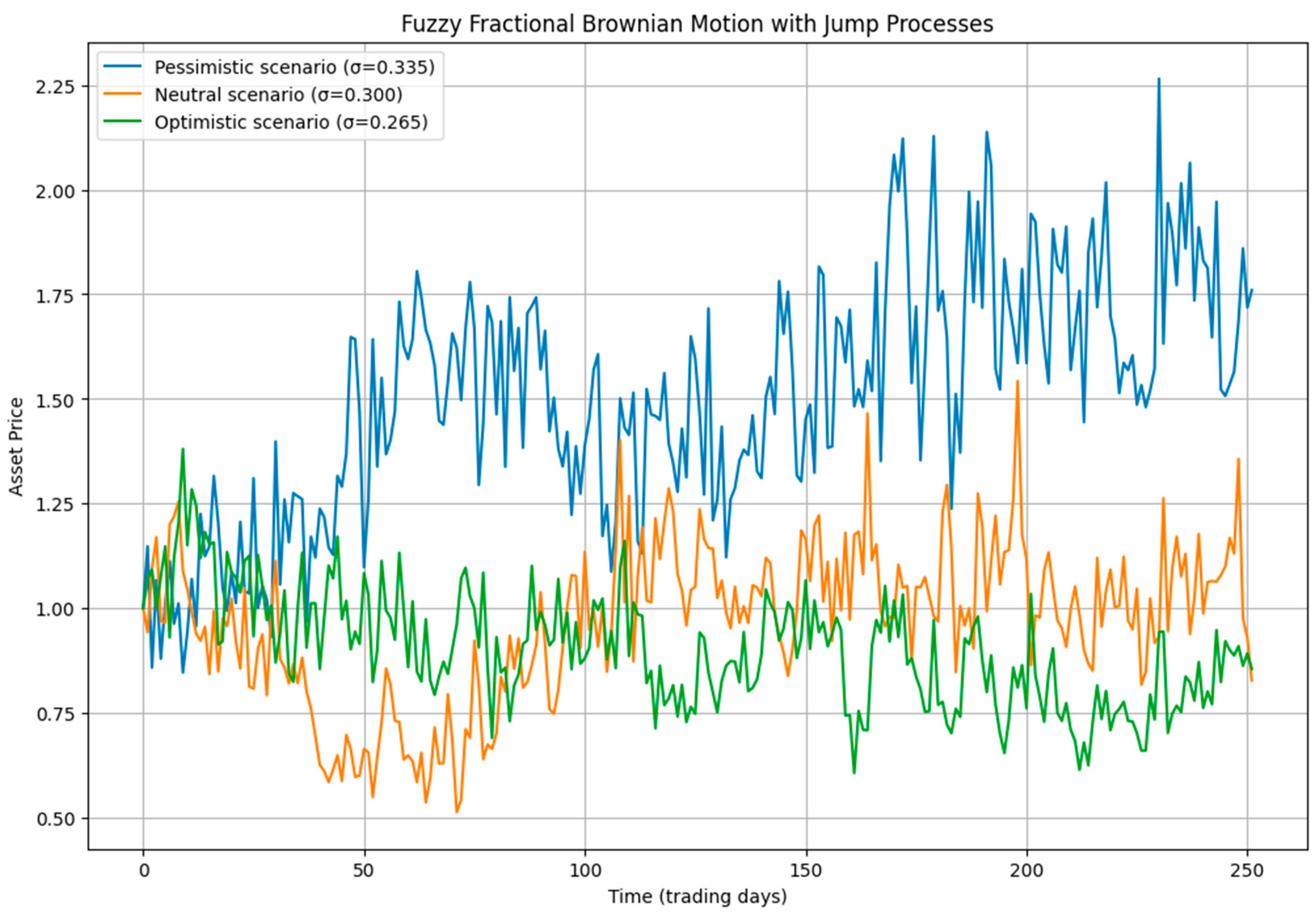
The techniques developed for fBm with H < ½ can be effectively applied in financial modelling, particularly in modelling volatility and volatility of volatility (vol-of-vol) which exhibit rough path structure [8,9]. These rough volatility models, often characterised by Hurst exponents less than ½, capture the persistent, jagged behaviour of market fluctuations more accurately. By incorporating fuzziness into key parameters such as volatility, drift, and jump intensities, the fuzzy fBm framework enhances the ability to model these irregularities and account for uncertainty in parameter estimation. This is particularly important in environments where precise volatility measurement is challenging due to market noise or incomplete data. The combination of fuzziness with rough fractional paths allows for a more robust representation of the volatility surface, improving option pricing, hedging strategies and risk assessment in volatile markets.

In the context of modelling volatility of volatility, the FFBM can be particularly useful in capturing the stochastic nature in instruments like VIX derivatives and volatility swaps. Traditional models often struggle to account for the irregular, long-memory effects present in vol-of-vol, which is now very documented in empirical finance [9]. By applying FFBM, empiricists can build a shifting vol-vol dynamic model without assuming an overly smooth process. As we demonstrated earlier, this framework can be integrated with Girsanov’s theorem under a risk-neutral measure, ensuring that the pricing of derivatives reflects real-world irregularities while maintaining theoretical robustness and no-arbitrage conditions.

In non-financial applications, a potential application is in the telecommunications and network traffic modelling. Fractional Brownian motion has already been widely used to model network traffic, but the real-world network conditions often exhibit variations that are best captured through fuzzy logic. In adaptive bandwidth allocation, congestion control, and network anomaly detection, FFBM can be employed to handle imprecise or incomplete traffic data, allowing service providers to develop more resilient protocols for managing data flow, reduce latency, and optimise resource allocation in high-traffic environments such as cloud computing and real-time streaming services.

In classical fBm, the kernel $K_H(t,s)$ governs the memory and roughness of the process through the Hurst exponent H. When fuzziness is introduced, the kernel becomes a fuzzy function. This means instead of having a single deterministic kernel, the model now handles sets of possible kernels defined by membership functions of fuzzy intervals. The amplitude functions, which influence the drift and diffusion terms in SDEs also become fuzzy variable. This means the diffusion coefficient σ and drift term μ are no longer fixed but represented by fuzzy sets or intervals. While fuzziness increases model complexity, it also introduces robustness in modelling real-world uncertainty. By modelling this uncertainty explicitly through fuzziness, the framework becomes mathematically richer and computationally more intensive, but these challenges are balanced by the model’s ability to capture real-world phenomenon where precise information is often unavailable or delayed.

3. Introducing Proof When H < ½

We will extend the proofs in [8] that are valid when H > ½. As we described it in the Introduction, fBm has an infinite quadratic variation when H < ½, so we use [12] to change Hurst parameter from H to 1 − H (Appendix A).

First, we use the following integration by parts result from [13]:

$${\int }_0^{T}f\left(t\right)d{B}^H\left(t\right)=f\left(T\right)B^H\left(T\right)-{\int }_0^T{B}^H\left(t\right)df\left(t\right)$$

The author proves the relationship for a deterministic function f such that it has bounded p-variation sample paths for all p < 1/(1 − H). Let $Y_t^H={\int }_0^t{s}^{H-{\displaystyle \frac{1}{2}}}d{B}^H\left(t\right)$. Then $B_t^H={\int }_0^t{s}^{H-{\displaystyle \frac{1}{2}}}d{Y}_s^H.$ Proof:

$$\begin{array}{l}{Y}_t^H={\int }_0^t{s}^{H-{\displaystyle \frac{1}{2}}}d{B}^H\left(t\right)\\ \hspace{1em}\hspace{1em}\hspace{1em}\hspace{1em}\hspace{1em}\hspace{1em}={\left(t\right)}^{{\displaystyle \frac{1}{2}}-H}{B}^H\left(t\right)\\ \hspace{1em}\hspace{1em}\hspace{1em}\hspace{1em}\hspace{1em}\hspace{1em}-{\int }_0^t{B}^H\left(t\right)d\left(t^{{\displaystyle \frac{1}{2}}-H}\right)=t^{{\displaystyle \frac{1}{2}}-H}{B}^H\left(t\right)-{\int }_0^t{B}^H\left(t\right)\left[{\displaystyle \frac{1}{2}}-H\right]t^{-{\displaystyle \frac{1}{2}}-H}dt\end{array}$$

Apply derivative:

$$\begin{array}{c}{dY}_t^H={({\displaystyle \frac{1}{2}}-H) t}^{-{\displaystyle \frac{1}{2}}-H}dt{B}^H\left(t\right)+d{B}^H\left(t\right)t^{{\displaystyle \frac{1}{2}}-H}-B^H\left(t\right)\left[{\displaystyle \frac{1}{2}}-H\right]t^{-{\displaystyle \frac{1}{2}}-H}=d{B}^H\left(t\right)t^{{\displaystyle \frac{1}{2}}-H}\\ \hspace{1em}\hspace{1em}\hspace{1em}\hspace{1em}\hspace{1em}\hspace{1em}\Rightarrow {dB}_t^H=d{Y}^H\left(t\right)t^{-{\displaystyle \frac{1}{2}}+H}\end{array}$$

Apply integration:

$$\Rightarrow B_t^H={\int }_0^t{s}^{-{\displaystyle \frac{1}{2}}+H}d{Y}^H\left(s\right)$$

(9)

Following notation from [14], we utilise Molchan martingale [15], $M_t^H :={\int }_0^{t}w(t, s){dB}^H\left(s\right)$, where $w\left(t,s\right)\doteq ({\displaystyle \frac{c}{C}})s^{-\alpha }{(t-s)}^{-\alpha }$ is a scaled beta kernel and w(t,s) = 0 for s > t; $\alpha \doteq H-{\displaystyle \frac{1}{2}}$; $C\doteq \sqrt{{\displaystyle \frac{H}{\left(H-\frac{1}{2}\right)B(H-\frac{1}{2}, 2-2H)}}}$ and $c\doteq {\displaystyle \frac{1}{B\left(H+\frac{1}{2}\right), (\frac{3}{2}-H)}}$. So, c(H) is a function of H and the standard Beta function $B\left(\mu , \upsilon \right)\doteq {\displaystyle \frac{\mathsf{\Gamma }\left(\mu \right)\mathsf{\Gamma }\left(\nu \right)}{\mathsf{\Gamma }(\mu +\nu )}}$. Using Proposition 2.1 from [14] and proof of Theorem of 3.2 in [16], then M is a Gaussian martingale. Put the values of dB into Molchan martingale we obtain:

$$M_t^H=({\displaystyle \frac{c}{C}}){\int }_0^t{s}^{{\displaystyle \frac{1}{2}}-H}{(t-s)}^{{\displaystyle \frac{1}{2}}-H}{s}^{H-{\displaystyle \frac{1}{2}}}d{Y}^H\left(s\right)=({\displaystyle \frac{c}{C}}){\int }_0^t{(t-s)}^{{\displaystyle \frac{1}{2}}-H}d{Y}^H\left(s\right).$$

Ref. [16] showed that the filtrations generated by M and Y are the same. They showed that $Y_T=2H{\int }_0^T{(T-t)}^{-{\displaystyle \frac{1}{2}}+H}dM\left(t\right)$ and the prediction formula:

$${E[Y}_T|F_t]=2H{\int }_0^t{(T-s)}^{-{\displaystyle \frac{1}{2}}+H}dM\left(s\right).$$

(10)

Now we use Equations (9) and (10) to find the upper bound using integration by parts. From (9):

$$\mathrm{s}\mathrm{u}\mathrm{p}|B_t^H|\le sup | {\int }_0^t{s}^{-{\displaystyle \frac{1}{2}}+H}d{Y}^H\left(s\right)|\le sup |{\left[s^{H-{\displaystyle \frac{1}{2}}}{Y}_s^H\right]}_0^T-{\int }_0^t{d(s}^{-{\displaystyle \frac{1}{2}}+H})Y^H\left(s\right)|$$

Since the integral term is positive, therefore:

$$\mathrm{s}\mathrm{u}\mathrm{p}|B_t^H|\le \mathrm{s}\mathrm{u}\mathrm{p}|{\left[s^{H-{\displaystyle \frac{1}{2}}}{Y}_s^H\right]}_0^T\le \sup \left|T^{H-{\displaystyle \frac{1}{2}}}\left(Y_t^H-Y_0^H\right)\right|\le 2T^{H-{\displaystyle \frac{1}{2}}}\sup \left|Y_t^H\right||$$

Now using (10), substitute for Y:

$$\begin{array}{l}\mathrm{s}\mathrm{u}\mathrm{p}|B_t^H|\le 2T^{H-{\displaystyle \frac{1}{2}}}\sup \left|2H{\int }_0^t{(t-s)}^{-{\displaystyle \frac{1}{2}}+H}d{M}^H\left(s\right)\right|\\ \hspace{1em}\hspace{1em}\hspace{1em}\hspace{1em}\hspace{1em}\hspace{1em}\le 2T^{H-{\displaystyle \frac{1}{2}}}2\mathrm{H}\mathrm{s}\mathrm{u}\mathrm{p}|{\left[{\left(t-s\right)}^{H-{\displaystyle \frac{1}{2}}}{M}_s^H\right]}_0^T-{\int }_0^t{d\left(\right(t-s)}^{-{\displaystyle \frac{1}{2}}+H})M^H\left(s\right)|\\ \hspace{1em}\hspace{1em}\hspace{1em}\hspace{1em}\hspace{1em}\hspace{1em}\le 4H{T}^{2H-1}\sup (\left|M_t^H\right|-|M_0^H\left|\right)\le 8H{T}^{2H-1}\sup (\left|M_t^H\right|)\end{array}$$

We now apply expectation:

$${\mathrm{E}(\sup \left|B_t^H\right|)}^p\le {\left(8H{T}^{2H-1}\right)}^p\mathrm{E}(\sup {\left(\left|M_t^H\right|\right)}^p)$$

Since M is Molchan martingale, by the Burkholder-Davis-Gundy inequality, there exists a constant $A_p^H>0$ such that:

$${\mathrm{E}(\sup \left|B_t^H\right|)}^p\le {\left(8H{T}^{2H-1}\right)}^p{A}_p^H\mathrm{E}(\sup {\left(〈M_t^H〉\right)}^{p/2})$$

(11)

The next result we take from Norros, Proposition 2.1 from [16]:

$$Var\left(M_t^K\right)={〈M^K〉}_t={\displaystyle \frac{c^2\left(K\right)}{{\left(2K\right)}^2(2-2K)}}{t}^{2-2K} :=d(K)t^{2-2k}$$

Now, we use the transformation proposed and proved by [12] to change Hurst parameter H. Using Corrollary 5.2 from [12], there exists a unique (1 − H) fBm, such that:

$$B_t^H={\left({\displaystyle \frac{2H}{\mathsf{\Gamma }\left(2H\right)\mathsf{\Gamma }(3-2H)}}\right)}^{1/2}{\int }_0^t{(t-s)}^{2H-1}d{B}_s^{1-H}, a.s., tϵ[0, T]$$

By remark 5.6 in [12], proves that:

$$M_t^H=\left(\sqrt{{\displaystyle \frac{1-H}{1-K}}}\right){\int }_0^t{s}^{K-H}d{M}_{s }^K, a.s., tϵ[0, \infty )$$

We will now combine these results to compute quadratic variation for 1 − H > ½ to obtain:

$$〈M_t^H〉={(\left(\sqrt{{\displaystyle \frac{1-H}{1-K}}}\right){\int }_0^t{s}^{K-H}d{M}_{s }^K) )}^2={\displaystyle \frac{1-H}{H}}{\int }_0^t{s}^{2-2H}{d〈M^{1-H}〉}_s$$

Use [16]: $Var\left(M_t^K\right)={〈M^K〉}_t={\displaystyle \frac{c^2\left(K\right)}{{\left(2K\right)}^2(2-2K)}}{t}^{2-2K}:=d(K)t^{2-2k}$.

Substitute into: $d{〈M^{1-H}〉}_s=d(1-H)s^{2-2(1-H)}$. Continuing with quadratic variation:

$$\begin{array}{l}〈M_t^H〉={(\left(\sqrt{{\displaystyle \frac{1-H}{1-K}}}\right){\int }_0^t{s}^{K-H}d{M}_{s }^K) )}^2={\displaystyle \frac{1-H}{H}}{\int }_0^t{s}^{2-2H}{d〈M^{1-H}〉}_s=\\ {\displaystyle \frac{1-H}{H}}d(1-H){\int }_0^t{s}^{2-2H}2H{s}^{2H-1}ds={\displaystyle \frac{2H\left(1-H\right)}{H}}d(1-H){\int }_0^t{s}^{1-2H}ds\\ \hspace{1em}\hspace{1em}\hspace{1em}\hspace{1em}\hspace{1em}\hspace{1em}=d(1-H)t^{2(1-H)}\end{array}$$

(12)

Apply BDG inequality on quadratic variation of M^H, to obtain:

$$E{\sqrt{{〈M^H〉}_t}}^p\le B_p^{1-H}{t}^{p(1-H)}$$

(13)

Using (11): ${\mathrm{E}(\sup \left|B_t^H\right|)}^p\le {(8H{T}^{2H-1})}^p{A}_p^H\mathrm{E}(\sup {\left(〈M_t^H〉\right)}^{p/2})$, substitute into (13), we obtain:

$${\mathrm{E}(\sup \left|B_t^H\right|)}^p\le {\left(8H{T}^{2H-1}\right)}^p{A}_p^H{B}_P^{1-H}{T}^{p(1-H)}$$

(14)

If we define $\mathrm{C}:={\left(8H\right)}^p{A}_p^H{B}_P^{1-H}$ then ${\mathrm{E}(\sup \left|B_t^H\right|)}^p\le C{T}^{pH}$. So, in summary, we use trick from [12] to transform fBm to (1 − H) fBm. By expressing fBm as an integral with respect to standard Brownian motion, the proof employs Volterra-like representations of fBm. The transformed process is a Gaussian martingale with respect to the filtration generated by B_H, which allows us to establish the upper and lower bounds for the integrals. Combined with the fact that we also demonstrate that the involved functions are square integrable, this ensures the finiteness and uniqueness of solution. Proof complete.

4. Introducing Fuzzy When H < ½

Under the assumption that the fuzzy aspect lives in the amplitude/kernels and that the underlying driving noise $\tilde{B}$ is actually a crisp fractional Brownian motion. In other words, we are layering fuzziness on the coefficients/functions of the integral but not changing the fundamental measure-theoretic structure of the noise. This assumption ensures we can leverage classical results such as Itô isometry for existence, uniqueness, and bounding integrals which we proved in [8].

For H < ½, the kernel K_H(t, s) used to construct fBm was derived by [17].

$$K_H\left(t,s\right)=c_H\left[{\left({\displaystyle \frac{t}{s}}\right)}^{H-1/2}{(t-s)}^{H-1/2}\right]$$

where C_H is a normalising constant given by: $c_H={\left({\displaystyle \frac{2Hsin\left(\pi H\right)\mathsf{\Gamma }(\frac{3}{2}-\mathrm{H})}{\mathsf{\Gamma }(H+\frac{1}{2})}}\right)}^{1/2}$.

For practical applications, a more convenient representation of the kernel function for H < ½ can be written as:

$$K_H\left(t,s\right)=c_H\left[{\left(t-s\right)}^{H-1/2}-{(-t)}^{H-1/2}\right]$$

This ensures the kernel remains well-defined and integrable. To establish upper and lower bounds for the integrals involving fuzzy fractional Brownian motion when H < ½, we need to adapt the existing techniques to handle the fuzzy nature of the random variables. To establish bounds, we need to represent the fuzzy variables as intervals or use membership functions and then analyse these representations.

An important characteristic of fBm that significantly enhances its applicability in financial modelling is its long memory effect, which is governed by the Hurst exponent H. The Hurst exponent characterises the autocorrelation structure of increments of the process. If H > ½, this indicates positive correlation and persistent behaviour, meaning past increases or decreases tend to be followed by future movements in the same direction. Financial assets exhibit persistent behaviour, and shocks to be positively correlated over long periods, making fBm an ideal model for capturing long-term dependencies observed in bubble dynamics.

If H < ½, this corresponds to anti-persistence, or rough path showing mean-reverting behaviour. Such anti persistence phenomena are frequently observed in short-term trading scenarios. In our context, we focus on the case of H < ½, as indicated above, due to its suitability for modelling frequent reversals.

Fuzzy Gaussian Distribution

At any fixed time t, the value of the fuzzy Brownian motion ${\tilde{B}}_H(t)$ is a fuzzy Gaussian variable. This means its probability distribution is a Gaussian distribution with fuzzy mean and variance.

Fuzzy Integral Representation:

We denote the kernel $K_H(t, s)$ as fuzzy, which means at each ω ∈ Ω, the kernel belongs to a set and has a membership function describing possible amplitude values.

$${\tilde{B}}_H(t)={\int }_0^t{\tilde{K}}_H(t, s)dB(s)$$

We assume the underlying noise is crisp, but the fuzzy aspect is in the amplitude of the kernel. We had earlier proven in [8] that the classical Itô isometry remains perfectly valid for each crisp selection and each scenario in our fuzzy ensemble because the noise is crisp. The fuzziness is layered on top by letting the integrand vary in intervals. Nothing breaks the standard measure-theoretic basis of ${\tilde{B}}_H(t)$.

Our future work would involve defining the fuzzy fractional Brownian motion ${\tilde{B}}_H\left(t\right)$ in the sense of fuzzy measure theory, not just a crisp B with fuzzy amplitude. Then the classical Itô isometry is no longer guaranteed. Indeed, we might not even have a linear–additive expectation E in the sense of Kolmogorov measure theory. Instead, we have fuzzy expectation and fuzzy integrals, which typically do not obey Itô isometry.

The step:

$$E\left[{\left({\int }_0^t\left({\tilde{K}}_H^{\left(1\right)}(t, s)-{\tilde{K}}_H^{\left(2\right)}(t,s)\right) d\tilde{B}(s)\right)}^2\right]\ne {\int }_0^{t}E\left[{{\widetilde{(K}}_H^{\left(1\right)}(t, s)-{\tilde{K}}_H^{\left(2\right)}(t,s))}^{2}ds\right]$$

would be wrong as indicated by ≠, because the left side uses a fuzzy integral and fuzzy expectation. Typically, a pure fuzzy measure does not preserve linear additivity, and it uses a non-classical integral Choquet, or Sugeno. The isometry is not guaranteed.

We need to analyse:

$$E\left[{\left({\widetilde{ B}}_H(t)\right)}^2\right]=E\left[{\left({\int }_0^t{\tilde{K}}_H(t, s)dB(s)\right)}^2\right]$$

Since both ${\tilde{K}}_H(t,s)$ and $\tilde{B}(s)$ are fuzzy, we can represent them as intervals for analysis.

The fuzzy labels on ${\tilde{K}}_H(t,s)$ does not break linearity or additivity of the expectations and the integrals, because fuzziness is above the measure level.

For uniqueness proofs, we define upper and lower bounds for Fuzzy Gaussian Increments:

$$\begin{array}{c}{\tilde{K}}_H(t,s)=\left[K_{H, L}(t, s), K_{H, U}(t, s) \right]\\ \tilde{B}(s)=\left[B_L\left(s\right), B_U\left(s\right)\right]\end{array}$$

Here, $K_{H, L}(t, s) \mathrm{a}\mathrm{n}\mathrm{d} K_{H, U}(t, s)$ represent the lower and upper bounds of the fuzzy kernel function, and $B_L\left(s\right) \mathrm{a}\mathrm{n}\mathrm{d} B_U\left(s\right)$ represent the lower and upper bounds of the fuzzy Gaussian process. The upper and lower bounds for the fuzzy fractional Brownian motion integrals are determined by analysing the bounds of the kernel function and the Gaussian process separately.

$${\left({\int }_0^t{\tilde{K}}_{H,L}(t, s)\right)}^{2}ds\le E\left[{\left({\int }_0^t{\tilde{K}}_H(t, s)d\tilde{B}(s)\right)}^2\right]\le {\left({\int }_0^t{\tilde{K}}_{H,U}(t, s)\right)}^{2}ds$$

By ensuring that these integrals are finite, we will demonstrate the existence of the solution. Uniqueness will be shown by proving that the fuzzy integrals converge uniquely under the given conditions—if that difference of kernels is zero a.s. owing to identical initial data and integrable constraints, we obtain uniqueness.

In other words, we need to show that:

$${\left({\int }_0^t{\tilde{K}}_{H,L}(t, s)\right)}^{2}ds<\infty \mathrm{and} {\left({\int }_0^t{\tilde{K}}_{H,U}(t, s)\right)}^{2}ds<\infty$$

For ${\tilde{K}}_{H,L}(t,s)$:

$${\left({\tilde{K}}_{H,L}(t, s)\right)}^2={c_H}^2{\left({(t-s)}^{H-1/2}-{(-s)}^{H-1/2}\right)}^2$$

Integrate this:

$${\int }_0^t{\left({\tilde{K}}_{H,L}(t, s)\right)}^{2}ds={c_H}^2{\int }_0^t{\left({(t-s)}^{H-1/2}-{(-s)}^{H-1/2}\right)}^{2}ds$$

Both terms inside the integral are finite for H < ½, and the subtraction term also ensures the finiteness of the integral.

Similarly, for the upper bounds:

$${\int }_0^t{\left({\tilde{K}}_{H,U}(t, s)\right)}^{2}ds={c_H}^2{\int }_0^t{\left({(t-s)}^{H-1/2}-{(-s)}^{H-1/2}\right)}^{2}ds$$

The same reasoning applies here, both terms inside the integral are finite, and their subtraction ensures the integrals are finite. Therefore, both the upper and lower bounds are finite.

To show uniqueness, we need to prove that the fuzzy integral representation converges uniquely under the given conditions. We assume that there are two fuzzy fractional Brownian motions ${\tilde{B}}_H^{\left(1\right)}(t)$ and ${\tilde{B}}_H^{\left(2\right)}(t)$ with the same initial conditions.

For uniqueness, consider the difference:

$${∆\tilde{B}}_H(t)={\tilde{B}}_H^{\left(1\right)}(t)-{\tilde{B}}_H^{\left(2\right)}(t)$$

Then:

$$E\left[{{∆\tilde{B}}_H(t)}^2\right]=E\left[{\left({\int }_0^t\left({\tilde{K}}_H^{\left(1\right)}(t, s)-{\tilde{K}}_H^{\left(2\right)}(t,s)\right) d\tilde{B}(s)\right)}^2\right]$$

Then we can use Itô’s isometry:

$$E\left[{{∆\tilde{B}}_H(t)}^2\right]={\int }_0^{t}E\left[{\left({\tilde{K}}_H^{\left(1\right)}(t, s)-{\tilde{K}}_H^{\left(2\right)}(t,s)\right)}^2\right]ds$$

If ${\tilde{B}}_H^{\left(1\right)}(t)$ and ${\tilde{B}}_H^{\left(2\right)}(t)$ are solutions, then ${\tilde{K}}_H^{\left(1\right)}(t,s)={\tilde{K}}_H^{\left(2\right)}(t,s)$ a.s. Thus, $E\left[{{∆\tilde{B}}_H(t)}^2\right]=0$.

This implies that ${∆\tilde{B}}_H(t)=0$ a.s. and ${\tilde{B}}_H^{\left(1\right)}(t)={\tilde{B}}_H^{\left(2\right)}(t)$. Proof complete. Therefore, the solution is unique.

Membership function:

$\tilde{X}$ is called a fuzzy normal variable if for each α ∈ (0, 1], we can select a crisp normal distribution $N\left({\mu }_{\alpha },{\sigma }_{\alpha }^2\right)$ such that μ_α and ${\mathsf{\sigma }}_{\mathsf{\alpha }}^2$ come from the α-cuts of the fuzzy numbers $\tilde{\mu }$ and $\widetilde{{\sigma }^2}$. The nested family $\{\mathrm{N}{\left({\mathsf{\mu }}_{\alpha },{\mathsf{\sigma }}_{\alpha }^2\right)\}}_{\alpha ϵ\left(0,1\right]}$ is consistent in the sense that if α₂ < α₁, then μ_α2 ⊆ μ_α1 as intervals.

Hence, we represent our fuzzy normal by the entire nested family of classical normal distributions, one for each level of membership α. Next, we apply the Zadeh extension principle (or an interval-based extension principle) to unify fuzzy parameters $\tilde{\mu }$ and $\widetilde{{\sigma }^2}$ into one membership function μ_X(x) for a fuzzy normal distribution. The key idea is once we have fuzzy sets for mean and variance, we want a single fuzzy set in R describing how likely it is for our fuzzy normal to take each real value x. This demands a recognised fuzzy extension approach that merges the fuzzy parameters into a single fuzzy set of real outputs. Generally, for each ${\alpha ⟶[\mu }_{\alpha },{\sigma }_{\alpha }^2]$ and t, the value ${\tilde{B}}_H(t)$ has membership function describing the degree to which it belongs to the fuzzy set ${\tilde{B}}_H(t)$.

$${\mu }_{\tilde{B}}=e^{-{\displaystyle \frac{{(x-\tilde{\mu })}^2}{2\widetilde{{\sigma }^2}}}}$$

When we have intervals of means μ ∈ $[{\mu }_{\alpha }^{-},{\mu }_{\alpha }^{+}]$ and variances σ ∈ $[{\sigma }_{\alpha }^{2,-},{\sigma }_{\alpha }^{2,+}]$, the pdf can vary accordingly. To find unified pdf we implement the threshold aggregator approach that merges the entire alpha-cut family into one membership function by allowing us to climb up alpha levels as far as possible, subject to the pdf condition. A bigger α indicates a narrower region for μ_α and ${\mathsf{\sigma }}_{\alpha }^2$, so it is more demanding that we still get bigger threshold in the pdf. The result is a single membership at x ∈ [0, 1]. If we define τ as some threshold then x has membership ≥ α if we can find a parameter pair in α-cuts that yields ≥ τ pdf. So, membership is the supremum of all such α. This is a version of the Zadeh extension principle, adopted to the pdf is above threshold τ condition.

We now formalise these concepts mathematically. Let $\tilde{\mu }$ be a fuzzy mean and $\widetilde{{\sigma }^2}$ be a fuzzy variance. $\tilde{\mu }$ and $\widetilde{{\sigma }^2}$ are fuzzy numbers in R and (0, ∞) respectively. Fix a threshold τ ∈ (0, ∞). For each α ∈ (0, 1], define intervals ${\mu }_{\alpha }ϵ{\tilde{\mu }}^{\alpha },{\sigma }_{\alpha }^2ϵ{{\tilde{\mu }}^2}^{\alpha }$.

We say x ∈ $\widetilde{X^{\alpha }}$ if:

$\exists \left(\mathsf{\mu },{\mathsf{\sigma }}^2\right)\in {\mathsf{\mu }}_{\alpha }\times {\mathsf{\sigma }}_{\alpha }^2$ such that $f_{\mu ,{\sigma }^2}(x)\ge \tau$.

Then the membership function for $\tilde{X}$ is:

$${\mathsf{\mu }}_{\tilde{X}}(\mathrm{x})=\mathrm{s}\mathrm{u}\mathrm{p}\{\mathsf{\alpha }\in (\mathrm{0,1}]:\mathrm{x}\in \widetilde{{\mathrm{X}}^{\alpha }}\}$$

We call $\tilde{X}$ a fuzzy normal variable under threshold τ.

This aggregator is one of many possible. Now we have a robust approach that merges fuzzy $\tilde{\mu }$ and $\widetilde{{\sigma }^2}$ into a single fuzzy set of real values x. It does so by checking the classical normal pdf at each α -cut and picking the supremum over α.

Fuzzy Martingale

A fuzzy martingale $\tilde{M}$(t) is a generalisation of a standard martingale, where the values are described by fuzzy numbers. For a process to be a fuzzy martingale, it must satisfy the martingale property with respect to fuzzy conditional expectations. So, for $\tilde{M}$(t) to be a fuzzy martingale, it must satify:

$$E\left[\tilde{M}|F_s\right]=\tilde{M}\left(\mathrm{s}\right)$$

Proof for Fuzzy Fractional Brownian motion when H < ½ with Gaussian membership function

We derive step by step proof for ffBm when H < ½ and Gaussian membership function.

1.

Integration by Parts with Fuzzy Variable:

Let ${\tilde{Y}}_t^H={\int }_0^t{s}^{H-{\displaystyle \frac{1}{2}}}d{\tilde{B}}^H\left(t\right)$. Then:

$${\tilde{B}}_t^H={\int }_0^t{s}^{H-{\displaystyle \frac{1}{2}}}d{\tilde{Y}}_s^H.$$

Our proof:

$$\begin{array}{l}{\tilde{Y}}_t^H={\int }_0^t{s}^{H-{\displaystyle \frac{1}{2}}}d{\tilde{B}}^H\left(t\right)\\ \hspace{1em}\hspace{1em}\hspace{1em}\hspace{1em}\hspace{1em}\hspace{1em}={\left(t\right)}^{{\displaystyle \frac{1}{2}}-H}{\tilde{B}}^H\left(t\right)\\ \hspace{1em}\hspace{1em}\hspace{1em}\hspace{1em}\hspace{1em}\hspace{1em}-{\int }_0^t{\tilde{B}}^H\left(t\right)d\left(t^{{\displaystyle \frac{1}{2}}-H}\right)=t^{{\displaystyle \frac{1}{2}}-H}{\tilde{B}}^H\left(t\right)-{\int }_0^t{\tilde{B}}^H\left(t\right)\left[{\displaystyle \frac{1}{2}}-H\right]t^{-{\displaystyle \frac{1}{2}}-H}dt\end{array}$$

Apply derivative:

$$\begin{array}{c}{d\tilde{Y}}_t^H={({\displaystyle \frac{1}{2}}-H) t}^{-{\displaystyle \frac{1}{2}}-H}dt{\tilde{B}}^H\left(t\right)+d{\tilde{B}}^H\left(t\right)t^{{\displaystyle \frac{1}{2}}-H}-{\tilde{B}}^H\left(t\right)\left[{\displaystyle \frac{1}{2}}-H\right]t^{-{\displaystyle \frac{1}{2}}-H}=d{\tilde{B}}^H\left(t\right)t^{{\displaystyle \frac{1}{2}}-H}\\ \Rightarrow {d\tilde{B}}_t^H=d{\tilde{Y}}^H\left(t\right)t^{-{\displaystyle \frac{1}{2}}+H}\end{array}$$

Apply integration:

$${\tilde{B}}_t^H={\int }_0^t{s}^{-{\displaystyle \frac{1}{2}}+H}d{\tilde{Y}}^H\left(s\right)$$

(15)

2.

Define fuzzy Molchan martingale:

$${\tilde{M}}_t^H:={\int }_0^t\tilde{w}(t,s){d\tilde{B}}^H\left(s\right),$$

where $\tilde{w}\left(t,s\right)\doteq ({\displaystyle \frac{c}{C}})s^{-\alpha }{(t-s)}^{-\alpha }$ is a scaled beta kernel.

3.

Upper bound for fuzzy ${\tilde{B}}_H(t)$ using integration by parts. From (15):

$$\mathrm{s}\mathrm{u}\mathrm{p}|{\tilde{B}}_t^H|\le sup | {\int }_0^t{s}^{-{\displaystyle \frac{1}{2}}+H}d{\tilde{Y}}^H\left(s\right)|\le sup |{\left[s^{H-{\displaystyle \frac{1}{2}}}{\tilde{Y}}_s^H\right]}_0^T-{\int }_0^t{d(s}^{-{\displaystyle \frac{1}{2}}+H}){\tilde{Y}}^H\left(s\right)|$$

Since the integral term is positive, therefore:

$$\begin{array}{l}\mathrm{s}\mathrm{u}\mathrm{p}|{\tilde{B}}_t^H|\le \mathrm{s}\mathrm{u}\mathrm{p}|{\left[s^{H-{\displaystyle \frac{1}{2}}}{\tilde{Y}}_s^H\right]}_0^T-{\int }_0^t(1/2-H)s^{-1/2-H} {\tilde{Y}}^H\left(s\right)ds|\\ \hspace{1em}\hspace{1em}\hspace{1em}\hspace{1em}\hspace{1em}\hspace{1em}\le \sup \left|T^{H-{\displaystyle \frac{1}{2}}}\left({\tilde{Y}}_t^H-{\tilde{Y}}_0^H\right)\right|\le 2T^{H-{\displaystyle \frac{1}{2}}}\sup \left|{\tilde{Y}}_t^H\right||\end{array}$$

4.

Now, substitute for $\tilde{Y}$:

$$\mathrm{s}\mathrm{u}\mathrm{p}\left|{\tilde{B}}_t^H\right|\le 8H{T}^{2H-1}\sup (\left|{\tilde{M}}_t^H\right|)$$

5.

We now apply expectation:

$${\mathrm{E}(\sup \left|{\tilde{B}}_t^H\right|)}^p\le {\left(8H{T}^{2H-1}\right)}^p\mathrm{E}(\sup {\left(\left|{\tilde{M}}_t^H\right|\right)}^p)$$

Since ${\tilde{M}}_t^H$ is a fuzzy Molchan martingale, by the Burkholder-Davis-Gundy inequality, there exists a constant $A_p^H>0$ such that:

$${\mathrm{E}(\sup \left|{\tilde{B}}_t^H\right|)}^p\le {\left(8H{T}^{2H-1}\right)}^p{A}_p^H\mathrm{E}(\sup {\left(〈{\tilde{M}}_t^H〉\right)}^{p/2})$$

(16)

The next result we take from Norros, Proposition 2.1 in [16]:

$$Var\left({\tilde{M}}_t^K\right)={〈{\tilde{M}}^K〉}_t={\displaystyle \frac{c^2\left(K\right)}{{\left(2K\right)}^2(2-2K)}}{t}^{2-2K} :=d(K)t^{2-2k}$$

6.

We will now combine these results to compute quadratic variation for 1 − H > ½ to obtain:

$$〈{\tilde{M}}_t^H〉={(\left(\sqrt{{\displaystyle \frac{1-H}{1-K}}}\right){\int }_0^t{s}^{K-H}d{\tilde{M}}_{s }^K) )}^2={\displaystyle \frac{1-H}{H}}{\int }_0^t{s}^{2-2H}{d〈{\tilde{M}}^{1-H}〉}_s$$

Use [16]: $Var\left({\tilde{M}}_t^K\right)={〈{\tilde{M}}^K〉}_t={\displaystyle \frac{c^2\left(K\right)}{{\left(2K\right)}^2(2-2K)}}{t}^{2-2K}:=d(K)t^{2-2k}$.

Substitute into: $d{〈{\tilde{M}}^{1-H}〉}_s=d(1-H)s^{2-2(1-H)}$. Continuing with quadratic variation:

$$\begin{array}{l}〈{\tilde{M}}_t^H〉={(\left(\sqrt{{\displaystyle \frac{1-H}{1-K}}}\right){\int }_0^t{s}^{K-H}d{\tilde{M}}_{s }^K) )}^2={\displaystyle \frac{1-H}{H}}{\int }_0^t{s}^{2-2H}{d〈{\tilde{M}}^{1-H}〉}_s=\\ ={\displaystyle \frac{1-H}{H}}d(1-H){\int }_0^t{s}^{2-2H}2H{s}^{2H-1}ds={\displaystyle \frac{2H\left(1-H\right)}{H}}d(1-H){\int }_0^t{s}^{1-2H}ds\\ \hspace{1em}\hspace{1em}\hspace{1em}\hspace{1em}\hspace{1em}\hspace{1em}=d(1-H)t^{2(1-H)}\end{array}$$

(17)

7.

Apply BDG inequality on quadratic variation of MH, to obtain:

$$E{\sqrt{{〈{\tilde{M}}^H〉}_t}}^p\le {\tilde{B}}_p^{1-H}{t}^{p(1-H)}$$

(18)

Using (16): ${\mathrm{E}(\sup \left|{\tilde{B}}_t^H\right|)}^p\le {(8H{T}^{2H-1})}^p{A}_p^H\mathrm{E}(\sup {(〈{\tilde{M}}_t^H〉)}^{p/2})$, substitute into (18), we get:

$${\mathrm{E}(\sup \left|{\tilde{B}}_t^H\right|)}^p\le {\left(8H{T}^{2H-1}\right)}^p{A}_p^H{\tilde{B}}_P^{1-H}{T}^{p(1-H)}$$

(19)

8.

If we define $\tilde{\mathrm{C}}:={\left(8H\right)}^p{A}_p^H{\tilde{B}}_P^{1-H}$ then ${\mathrm{E}(\sup \left|{\tilde{B}}_t^H\right|)}^p\le \tilde{C}{T}^{pH}$. Proof complete.

The risk-free measure transformation relies on constructing a risk-neutral probability measure under which the discounted asset price processes become martingale. In our fuzzy environment, the validity of this transformation hinges upon the assumption that fuzziness is introduced at the coefficient and amplitude level as opposed to altering the fundamental probability measure structure itself. Since the driving noise remains crisp, the classical construction of the risk-free measure is preserved. Thus, each scenario within our fuzzy environment still respects the standard probabilistic assumptions required by the Girsanov transformation.

In order to generalise the classical Girsanov transformation to cover fBm by leveraging Molchan-Golosov representation and a suitable martingale constructions. This extension ensures the stochastic integrals driven by fBm can be translated into equivalent martingale measures, allowing us to consistently price financial derivatives under fuzzy fractional dynamics. The generalisation uses fractional kernels and transformations introduced through fuzzy integral bounds. To illustrate the practical implications, consider the following heuristic numerical example involving a European call option.

Assumptions:

• Asset Price, S₀: 100
• Strike Price K: 100
• Risk-Free Rate: 0.05
• Time to maturity (T): 1.0 year(s)
• Hurst Exponent H: 0.4
• Adjusted Volatility Interval (fuzzy): [0.1500, 0.2500]
• Drift (fuzzy), μ: [0.04, 0.08]

Results under lower bound and upper bound scenarios:

• Option Price Interval: [8.5917, 12.3360]

5. Simulations

This simulation integrates three distinct components—fBm, Poisson jump processes, and fuzzy set theory to represent asset price dynamics under uncertainty and rough volatility scenario. Fbm was generated with a H = 0.15, specifically selected to reflect the rough volatility observed empirically in the financial markets. A low Hurst exponent captures anti-persistent behaviour, manifesting as rough paths with rapid, irregular fluctuations. The path was simulated over a one-year period (T = 1) using 252 discrete time steps, corresponding to typical daily trading intervals in financial markets. The simulation used Cholesky decomposition applied to a covariance matrix (γ), which encodes the long-range dependency structure of fBm increments.

Next, a jump component was added using a Poisson jump model, where the jump intensity parameter λ = 0.5 signifies an average occurrence of 0.5 jumps per year. Jump sizes were normally distributed with mean (μ = 0.5) and standard deviation (σ = 0.02), simulating occasional significant market shocks or discontinuities.

To incorporate market uncertainty and sentiment explicitly, the volatility parameter was dynamically adjusted using fuzzy logic. The fuzzy logic system defines three market sentiment scenarios–pessimistic, neutral, and optimistic, mapped numerically within a sentiment range from 0 to 10. The fuzzy volatility was obtained by evaluating these sentiment scenarios through fuzzy membership functions defined using triangular fuzzy sets. Specifically, pessimistic sentiment corresponds to high volatility, neutral sentiment to medium volatility, and optimistic sentiment to low volatility. This approach allowed the volatility parameter to be dynamically adjusted according to fuzzy logic, capturing the nuanced market sentiment and uncertainty explicitly.

The simulated asset price paths in Figure 1 were constructed by combining the drift by setting a constant risk-free rate of 5%, fuzzy-adjusted volatility, fBm paths, and cumulative jump increments. The resulting price series this explicitly illustrates the interactions among fractality captured by fBm, discrete jumps captured by Poisson jump processes, and fuzzy uncertainty via volatility adjustments from fuzzy set theory.

It is important to highlight that the simulation serves as an illustrative example to demonstrate the practical integration and behaviour of fBm, Poisson jumps, and fuzzy logic within our theoretical framework. Future work will explicitly perform extensive empirical validations, applying this modelling framework across various financial markets and directly comparing its predictive accuracy and performance against traditional models.

6. Discussion

The fractional fuzzy stochastic differential equations developed in this study provide a versatile framework that adapts to a variety of financial markets by capturing long-memory properties and uncertainty through fBm and fuzzy set theory, respectively. The flexibility of the model lies in its ability to accommodate diverse market behaviours by adjusting H and the fuzzy structure applied to the model’s coefficients.

In equity markets, where persistence and long-memory are often observed, our model with H > ½ offers significant advantages. Such markets tend to exhibit trends that persist over time, and this memory effect is well-captured using fractional dynamics. The introduction of fuzzy elements into volatility and drift parameters allows the model to integrate uncertainties arising from market shocks, incomplete financial information, or regulatory ambiguities. Empirical studies by Mandelbrot and van Ness, among others, have shown that equity prices frequently follow such persistent patterns, making our approach particularly well-suited for equities exhibiting trend following behaviour.

In foreign exchange and currency markets, price trajectories tend to alternate between memory effects and high-frequency volatility spikes. By integrating fuzzy processes with fractional models, we provide a framework that addresses these idiosyncrasies. The model’s flexibility allows it to accommodate changing market regimes, as well as uncertain monetary policies or geopolitical factors that are not easily handled by traditional diffusion-based models.

For commodity markets, which often exhibit mean-reverting characteristics, our model proves equally applicable. When H < ½, the model captures the cyclical, anti-persistent nature of commodity movements.

The main structural advantage of our customised PDE lies in its formulations, which incorporates exponential functions under positive drive scenarios (μ ≥ 0) and hyperbolic functions (cosh and sinh) when modelling regime with negative drive (μ ≥ 0). This dual structure allows the model to capture both compounding growth processes and cyclical market behaviours under a single unified framework. In contrast, classical PDEs based on standard Brownian motion typically assume memoryless behaviour and constant volatility, limiting their ability to capture persistent volatility clustering or regime-switching phenomena observed in empirical financial data.

To demonstrate the practical advantages of this model, we included a numerical example illustrating the pricing of a European call option under fuzzy volatility intervals derived from fBm dynamics. The results show how incorporating fuzziness yields a distribution of option prices, thereby providing a range of risk-adjusted values rather than a single deterministic price. This enriches the information available to market practitioners, supporting hedging and risk management under uncertainty.

Finally, classical models such as Black-Scholes-Merton [18] often underestimate pricing bounds under extreme uncertainty, our approach adapts to market-specific features like long memory, uncertainty in inputs, and non-Gaussian effects, delivering improved pricing accuracy and risk estimates. Therefore, this hybrid model shows strong potential for practical use in markets where classical assumptions on memory and volatility independence are no longer valid.

7. Conclusions

We formalised the study of a fuzzy fractional Brownian motion (fBm) for H < ½ by adapting classical results from traditional fBm setting, while layering fuzziness on certain coefficients and amplitude functions. In the crisp scenario, fBm with H < ½ is often represented via the Mandelbrot–Van Ness construction, where B^H(t) is expressed as an integral of a kernel K_H(t, s) against a standard Brownian motion. This kernel typically takes a difference form that remains integrable near the endpoints s = 0 and s = t, even though the process is not a semimartingale. To extend this into a fuzzy framework, we assumed that the driving fractional Brownian motion is still a classical, measure-theoretic process, but the kernel and other amplitude-related parameters become fuzzy. This framework allowed us to reuse many of the standard measure-theoretic techniques for integrals and isometries, because the underlying noise retained all its crisp characteristics.

We treated the kernel and the parameters as fuzzy sets whose possible values, for each outcome, lie in the intervals or have membership functions describing their degrees of plausibility. Each realisation of these fuzzy parameters can then be viewed as a crisp selection, ensuring the integral with respect to the standard Brownian motion is well-defined in the usual sense. This framework allows the preservation of existence, uniqueness, and boundedness properties. The driving noise is classical, so measure-theoretic arguments like the Young and Skorohod integrals for H < ½ continue to hold, and the presence of fuzziness in the amplitude and kernel does not break the underlying integrability conditions.

A key aspect of analysis focuses on uniqueness. If two processes ${\tilde{B}}_H^{\left(1\right)}(t) \mathrm{a}\mathrm{n}\mathrm{d} {\tilde{B}}_H^{\left(2\right)}(t)$ share the same fuzzy kernel data but happen to differ in how one selects fuzzy values for the integrand, one looks at their difference ${∆\tilde{B}}_H(t)$. Because the underlying noise is a crisp Brownian motion, one applies the standard isometry. If $\widetilde{K_{H, L}}(t, s) \mathrm{a}\mathrm{n}\mathrm{d} \widetilde{K_{H, U}}(t, s)$ coincide almost surely in the sense that their fuzzy parameters are identical for each scenario, then the difference integral is zero. This shows that no two distinct fuzzy processes can arise from the same fuzzy kernel data, and uniqueness is secured.

To bound the supremum of fuzzy fBm, we employed a form of the Molchan martingale technique and a BDG inequality approach [19]. In standard fBm with H < ½, one can define a transform that behaves like a martingale with respect to a certain filtration or at least allows one to control the magnitude of B^H(t). By retaining a crisp measure for the noise, the same style of arguments holds. We obtained an estimate of $sup|{\tilde{B}}_t^H|$ in terms of $\mathit{sup}(\left|{\tilde{M}}_t^H\right|)$, where ${\tilde{M}}_t^H$ is a fuzzy version of the Molchan martingale. Expectation inequalities follow from standard integrability requirements.

Taken together, we showed that working with H < ½ in the fuzzy context does not fundamentally destroy the usual integrability results, as long as the driving noise remains crisp. The main difference is that each amplitude or kernel value now belongs to a fuzzy set, but any specific scenario or selection yields a classical integrand, so integral definitions and uniqueness proofs proceed as in the standard framework. The bounding arguments are similar. We reused the classical measure-theoretic inequalities and simply recognised that the fuzziness entered in the amplitude, not in the measure. In this way, the entire theory remained consistent for H < ½, including existence of the fuzzy fractional Brownian motion, its uniqueness from the integral representation plus the crisp isometry argument, and the ability to label its distribution as fuzzy Gaussian via alpha-cuts and an aggregator principle.

The concept of overlaying a fuzzy structure onto a crisp fractional Brownian motion is not entirely new. Various authors in fuzzy stochastic modelling that we thoroughly reviewed in [8] have taken a crisp process such as a Brownian motion or a fractional Brownian motion and allowed certain parameters or coefficients to be fuzzy, thus letting each outcome pick a different crisp coefficient from the fuzzy set. This approach makes it possible to reuse all the standard measure-theoretic arguments, because the noise is still treated in a classical Kolmogorov framework.

However, systematically applying this method in the specific case of H < ½ for fractional Brownian motion, together with an explicitly defined aggregator and Zadeh extension principle for fuzzy normal distributions, has not been formalised in the literature. Mostly, research focuses on a fully crisp version of fractional Brownian motion in the non-semimartingale regime without considering fuzziness, or it addresses fuzzy Brownian motion or fBm in a more informal manner without fully elaborating measure-theoretic integrals or the precise aggregator rules that unify fuzzy parameters into one membership function on the real line [20,21,22]. Some articles instead mention fuzzy parameters in simpler SDE frameworks with Brownian noise but do not carefully handle the fractional exponents and the integration approach required for H < ½ [23,24,25,26,27,28,29,30,31,32].

Our research offers a unified formalism for adapting the fractional integral representation when H < ½, how to treat fuzzy kernel and amplitude values while preserving the crisp measure structure of the noise, and demonstrating existence, uniqueness, and boundedness in that environment. We clarified how to use the classical fractional integral machinery in a fuzzy setting, employed the standard uniqueness arguments while acknowledging the fuzziness of the kernel, and explained how to define a fuzzy normal membership function rather than simply stating fuzzy Gaussian without formal details. The originality of our approach lies in its explicit handling of the non-semimartingale regime H < ½ within a fuzzy kernel environment, its maintenance of the validity of measure-theoretic integrals by keeping the noise crisp, and its articulation of a consistent approach to defining the distribution via a recognised aggregator principle for fuzzy normals. Our rigorous treatment of fuzzy fractional Brownian motion and a clear explanation of how fuzziness modifies the usual uniqueness proofs and distribution membership constitute a coherent roadmap that is currently missing in the existing literature.

Our rigorous treatment of fBm and a clear explanation of how fuzziness modifies the usual uniqueness proofs and distribution membership constitutes a coherent roadmap that is currently missing in the existing literature. Furthermore, our model demonstrates superior applicability to financial products where long-term dependency and uncertainty are critical. In particular, it provides improved performance in pricing and hedging options with persistent volatility or mean-reverting characteristics which are common in equity indices and commodity markets, respectively. By incorporating fuzzy fractional dynamics, the model captures both long memory and uncertainty, offering more realistic pricing intervals and enhanced risk assessments compared to classical models. These attributes make the model highly relevant not only for option pricing but also for broader derivative applications and risk management strategies, where accurate quantifications of volatility ambiguity and drift uncertainty is essential.