Mirror Complementary Triplet Periodicity of Dispersed Repeats in Bacterial Genomes

Abstract

We investigated overlapping dispersed repeats (DRs) on the plus and minus DNA strands in 12 bacterial genomes. The use of the iterative procedure method (IP method) without taking into account insertions or deletions of nucleotides allowed speeding up the calculations by several times and increased the number of the identified DRs by 10–20%. Most of the DRs were found in the known bacterial genes. The intersection regions of the bacterial DRs contained reverse complement codons. Calculation of triplet periodicity matrices mt(i,j) (i is the position in the codon and j is the nucleotide) was performed for the intersection regions. Two classes of matrices in which the number of nucleotides was significantly greater than in random sequences were revealed: the first contained mt(1,G), mt(2,A), mt(2,T), and mt(3,C) cells and the second mt(1,G), mt(2,C), mt(3,A), and mt(3,T) cells. These classes included 10 and 2 bacterial genomes, respectively. The reverse complement transformation of the DR intersection regions preserved the cells in both classes, although cyclic matrix shifting to the right by one base was observed in the second class. The reverse complement codons in the DR intersection regions on the plus and minus DNA strands could represent sites of more frequent inversions/transpositions or participate in the formation of secondary/tertiary mRNA structures.

1. Introduction

Active development of methods for genome sequencing in the past decades resulted in the accumulation of more than 25 trillion base pairs and 3.7 billion nucleotide sequences according to the 2024 Genbank update [1]. Among them, the number of sequenced bacterial genomes exceeds 500,000 [2]. Analysis of the huge amount of genetic data obtained by sequencing requires the development of new, more sophisticated mathematical methods [3], which have already been successfully applied to the identification of dispersed DNA repeats in both eukaryotic and prokaryotic genomes. Dispersed repeats (DRs) are DNA fragments with certain similarity that are scattered throughout the genome and can vary in length from several hundred to several thousand bases [4,5]. In mammalian genomes, the proportion of DRs ranges from 25 to 50% [6], whereas in prokaryotic genomes their ratio is significantly lower [7,8]. Compared to eukaryotes, bacteria and archaea have small compact genomes, 85–90% of which encodes proteins or stable RNA molecules; the rest represents regulatory sequences. Since there are few chromosomal regions devoid of functional constraints, prokaryotic genomes can contain only a small number of repetitive elements.

The mathematical methods to search for DRs can be divided into two groups [9]. The first includes algorithms that find DRs based on the repeat sequences deposited in the databases. This class is represented by such programs as RepeatMasker [10], Censor [11], MaskerAid [12], and some others; they often use Repbase [13] as a reference database. Although these methods are successfully applied to identify already known DRs in the newly sequenced genomes, they are not effective in finding previously unknown DR sequences.

The search for new DR families is usually carried out by the mathematical algorithms of the second group including Recon [14], PILER [15], RepeatScout [16], and RepeatFinder with REPUter [17], which find DRs de novo. However, these methods have a significant limitation as they can identify only very similar repeats, i.e., those that have not accumulated many base substitutions. These methods can correctly detect DR families if the average number of substitutions per nucleotide (x) in their members does not exceed 1.0 (x ≤ 1.0) [18] but are unable to find DRs with x > 1.0. To address this problem, we have recently developed the iterative procedure (IP) method which allows the detection of DRs with x ≤ 1.7 [19]. The IP algorithm, which includes the construction of position-weight matrices (PWMs), iterative procedure, and dynamic programming, can obtain a matrix characteristic for a DR family existing in the bacterial genome and identify new DNA repeats.

The application of the IP method has made it possible to detect DR families in the genomes of bacteria from 42 phyla [19]. Our previous results indicate that each analyzed microbe contains at least one large DR family which occupies from 17 to 72% of the genome; the repeats are about 500 DNA bases long and most of them demonstrate triplet periodicity [20]. Triplet periodicity is a property inherent to many genes [20], and since the majority of DRs are parts of bacterial coding sequences, they also show periodicity. Let us explain the assessment of the periodicity on the example of DR sequence s(j), where j varies from 1 to L (repeat length). Periodicity is considered when in each repeat, frequency mt(i,k) statistically significantly differs from frequency e(k); k has values {a, t, c, g}, i = j − 3int((j − 0.1)/3) (i = 1, 2, 3, 1, 2, 3, …), and matrix mt(i,k) has the dimension 3 × 4. Then, mt(i,k) and e(k) are filled iteratively as mt(i,s(j)) = mt(i, s(j)) + 1 and e(s(j)) = e(s(j)) + 1 for all j = 1, 2, …, L. As a statistical measure of the difference, it is convenient to take mutual information I since its doubled value has an χ² distribution with 6 degrees of freedom [21], which allows a relatively easy filtering out of insignificant triplet periodicity. We have also observed that in bacterial genomes, DRs on the plus and minus DNA strands are positioned mostly in the same genomic areas, indicating their intersection.

The aim of this study was to investigate overlapping DRs on the plus and minus DNA strands of 12 bacterial genomes and determine DR characteristics responsible for the overlap. To this purpose, we used the IP method without dynamic programming, which made it possible to exclude from the search DRs with nucleotide insertions and deletions. Consequently, the calculation process was accelerated by several times and the number of statistically significant DRs identified in the bacterial genome was increased by approximately 10–20%. Most of the detected DRs were located in the known bacterial genes. We found that the intersected regions of the DRs in bacterial genomes contained reverse complement codons (RCCs) and had triplet periodicity falling into two groups. In the first, the number of nucleotides in cells mt(1,G), mt(2,A), mt(2,T), and mt(3,C) was significantly greater than could be expected for random sequences; it comprised 10 genomes, including that of E. coli. In the second group, the number of nucleotides in cells mt(1,G), mt(2,C), mt(3,A), and mt(3,T) was greater than expected for random sequences. If the intersection region of the DR was flipped by 180 degrees and the bases were recoded to the complementary ones, then in the first group cells mt(1,G), mt(2,A), mt(2,T), and mt(3,C) were preserved. The same happened in the second group but with a cyclic shift in matrix mt(i,k) to the right by one base. We also discuss the possible functional significance of the found DRs and the presence of RCCs in the intersecting DR regions on the plus and minus DNA strands.

2. Materials and Methods

2.1. IP Method to Identify DRs in Bacterial Genomes

To search for DRs, we used the IP method [18,19] without dynamic programming so that it detected DRs without nucleotide insertions or deletions. The algorithm diagram is shown in Figure 1. Let us take a quick look at how the IP method works without dynamic programming. The algorithm of IP method included three stages. I. Generation of random PWMs of 600 DNA bases long; each matrix had 600 columns and 16 rows and was filled with the numbers showing the weight of each pair of adjacent bases in each column of the matrix. II. Conduction of the IP search for DRs in the bacterial genome using the created PWMs. III. Evaluation of the statistical significance of the found similarities. These stages are described in detail below.

2.1.1. Generation of Random PWMs

To obtain random PWMs, we constructed set Q_r containing K = 100 random sequences S_r of length L = 600 DNA bases and created numerical sequence S_n containing numbers from 1 to L in the ascending order. Then, we filled in matrices M(16, L) as follows:

m(t(i), s_n(j)) = m(t(i), s_n(j)) + 1

(1)

Here, m denotes a cell of matrix M, t(i) = $s_r^k$(i − 1) + 4$s_r^k$(i), $s_r^k$(i) is the nucleotide at position i in sequence number k from set Q_r, and s_n(j) is the number at position j in sequence S_n; k varies from 1 to K, i—from 2 to L and j—from 1 to L. After filling matrix M, we calculated random PWM(16, L) as follows:

$$PWM\left(i,j\right)={\displaystyle \frac{M\left(i,j\right)-Np(i,j)}{\sqrt{Np(i,j)(1-p(i,j))}}}$$

(2)

where p(i,j) = x(i)y(i)/N², $x(i)={\displaystyle \sum _{j=1}^{L}M(i,j)}$, $y(j)={\displaystyle \sum _{i=1}^{16}M(i,j)}$, and $N={\displaystyle \sum _{i=1}^{16}{\displaystyle \sum _{j=1}^{L_1}M(i,j)}}$. Then, the PWM was transformed so that sum $R^2={\displaystyle \sum _{i=1}^{16}{\displaystyle \sum _{j=1}^{L_1}pwm}}{(i,j)}^2$ retained constant value $R_0^2$ for all matrices which were used below to find similarity between the PWM and the analyzed sequence S (matrix transformation procedure is described in detail in [22]. For the transformed matrices, sum $K_d={\displaystyle \sum _{i=1}^{16}{\displaystyle \sum _{j=1}^{L_1}pwm}}(i,j)p_1(i)p_2(j)$ was also maintained equal to K₀. In this formula, pwm(i,j) is the element of the PWM located on the i-th row and j-th column, p₂(j) = 1/L, and p₁(i) = f(k)f(l), where f(k) is the probability of a nucleotide of type k and f(l) is the probability of encountering a nucleotide of type l in the analyzed sequence S (k and l can be A, T, C, or G). The (k,l) pair forms index i which varies from 1 to 16. In this study, we used parameters L = 600, K₀ = −1.0, and R₀ = 126 × 10³; K₀ = −1.0 allows accurate determination of the beginning and end of the local alignment [22] between the PWM and sequence S₁ (see Section 2.2).

After creating one PWM(16, L), we repeated all the calculations described above and obtained a set of such matrices denoted as W, which contained 100 PWM(16, L).

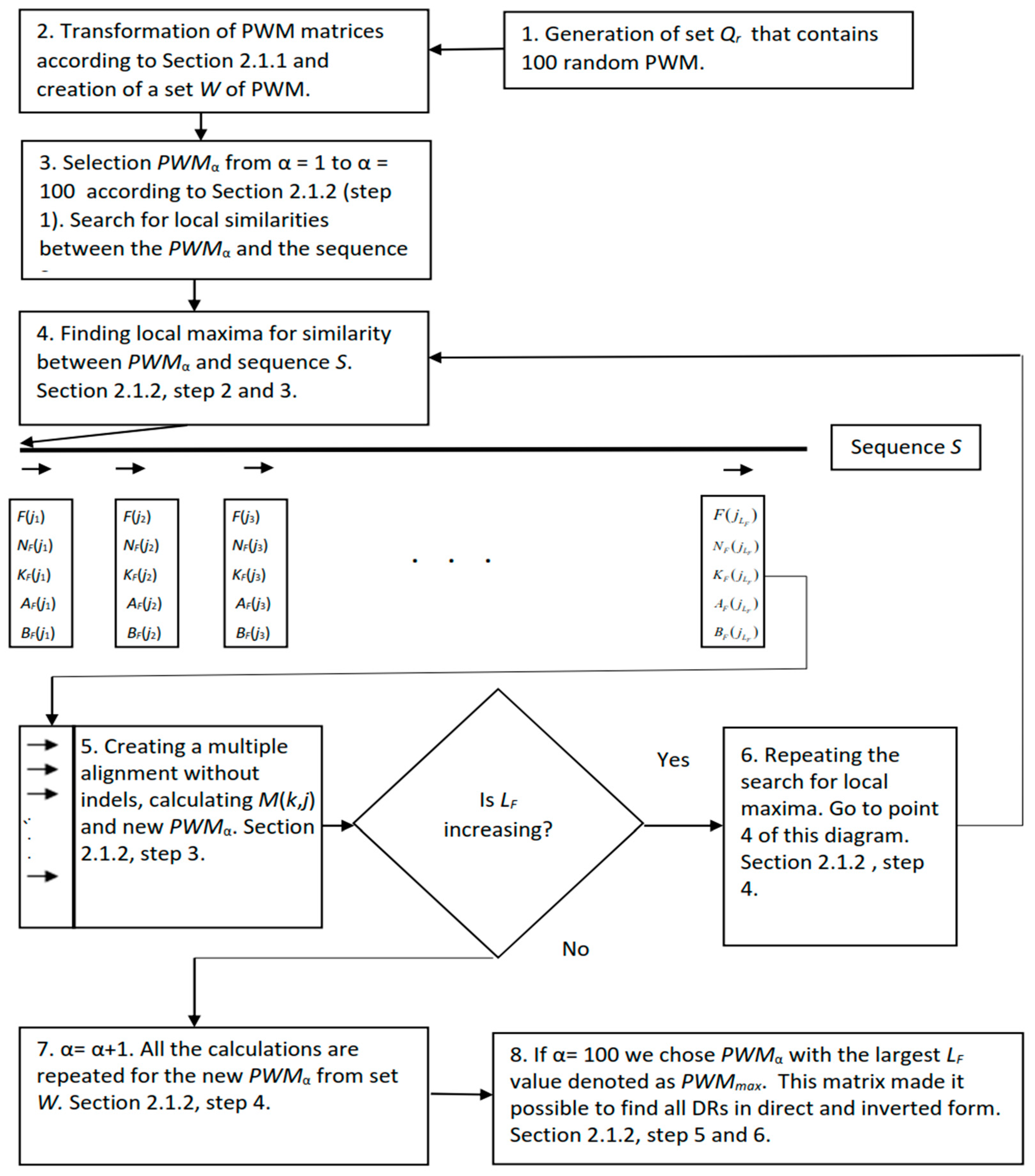
2.1.2. Iterative Procedure to Search for DRs Using Matrices of Set W

Step 1. To find DRs in the bacterial genome sequence denoted as S, we started with the first matrix from set W, which was denoted as PWM_α (α = 1). Then, for each base number j in sequence S (starting with j = 1), we calculated V(j + h) as follows:

$$V(j+h)=\max \left\{\begin{array}{l}V(j+h-1)+PW{M}_{\alpha }(t(h),s_n(h))\\ 0\end{array}\right\}$$

(3)

Here, α is the number of a PWM in set W and t(h) = s(j + h − 1) + 4s(j + h), where s(j + h − 1) and s(j + h) are the elements of sequence S and s_n(h) is the element of sequence S_n (Section 2.1.1). Then, among all h (which varied from 2 to 600), we determined the maximum value of function V(j + h), which was V_max(j). The coordinates of V_max(j) in sequences S and S_n were denoted as K_max(j) and A_max(j), respectively. We moved from K_max(j) towards j + 2 by decreasing h and searched for the first value of V(j + h) equal to zero; this coordinate in sequence S was denoted as N_max(j) and in sequence S_n—as B_max(j). The calculations were repeated for j from 1 to L_s−599, where L_s was the length of sequence S.

Step 2. As a result of these calculations, we obtained the values of V_max(j), N_max(j), K_max(j), A_max(j), and B_max(j). Next, we sorted vector V_max(j) in a descending order and obtained vector V_dec(i), where V_dec(1) was the largest value. For each V_dec(i), we took the corresponding values of N_max(j), K_max(j), A_max(j), and B_max(j) denoted as N_dec(i), K_dec(i), A_dec(i), and B_dec(i), respectively (here, i also varied from 1 to L_s−599), and selected only those V_dec(i) values for which the sequences from N_dec(i) to K_dec(i) did not intersect. The selection process started with V_dec(1) and the coordinates of N_dec(1) and K_dec(1). Then, we created F(1) = V_dec(1) and N_F(1) = N_dec(1), K_F(1) = K_dec(1), A_F(1) = A_dec(1), and B_F(1) = B_dec(1) and further considered only those V_dec(i) for which N_dec(i) ≥ K_F(1) or K_dec(i) ≤ N_F(1), excluding all other V_dec(i) values. Among the remaining V_dec(i), we found the maximum, made F(2) equal to this value, and wrote the corresponding coordinates in N_F(2), K_F(2), A_F(2), and B_F(2). Again, we left only those V_dec(i) values for which N_dec(i) ≥ K_F(2) or K_dec(i) ≤ N_F(2) and excluded all the rest. This process was continued until vector V_dec(i) was greater than V₀ (calculation of V₀ is described below in Section 2.1.3). As a result, we obtained vector F(j) and the corresponding N_F(j), K_F(j), A_F(j), and B_F(j); here, j varied from 1 to a certain L_F value, which was unknown beforehand.

Step 3. After these calculations, we constructed multiple alignment for all sequences j from 1 to a certain L_F value, which had coordinates from N_F(j) to K_F(j). The nucleotides belonging to any column of the multiple alignment were selected from sequence S_n within coordinates from A_F(j) to B_F(j). For example, if a nucleotide sequence with coordinates N_F(j) to K_F(j) from sequence S is ATCCGG and its A_F(j) and B_F(j) coordinates are 401–406, then nucleotide A falls in column 401, T in column 402, etc.; the last nucleotide G falls in column 406. Columns from 1 to 400 and 407 to 600 are filled with the “-” symbol.

In this way, we completely filled in the matrix for multiple alignment, which had 600 columns and L_F rows and was denoted as MM(i,j) (i varied from 1 to L_F and j from 1 to 600). Then, we filled in frequency matrix M(k,j) (k from 1 to 16 and j from 2 to 600) as m(t(i), j) = m(t(i), j) + 1, where m was the cell of matrix M, t(i) = mm(i,j − 1) + 4mm(i,j), and mm(i,j) was the nucleotide at position i,j in matrix MM. If mm(i,j) or mm(i,j − 1) contained symbol “-”, then the calculations were not performed. This iterative procedure was conducted for all i from 1 to L_F and j from 1 to 600.

Step 4. After defining matrix M(k,j), we calculated the PWM using Formula (2) (Section 2.1.1) and modified it so that K₀ = −1.0 and R₀ = 126 × 10³. Then, we returned to Formula (3) and repeated all the calculations. The cycle was stopped when the L_F value ceased increasing and started decreasing. As a result of these cyclic calculations, we obtained new matrix PWM_α instead of the original matrix PWMα and used the former to calculate F(j), N_F(j), K_F(j), A_F(j), and B_F(j).

Step 5. All the calculations were repeated for the new PWM_α from set W for α from 1 to 100. At the end, we chose PWM_α with the largest L_F value denoted as PWM_max. This matrix corresponded to F(j), N_F(j), K_F(j), A_F(j), and B_F(j), where j varied from 1 to L_F; here, F(j) is the weight of the match between the j-fragment of sequence S from N_F(j) to K_F(j) and the fragment of sequence S_n from A_F(j) to B_F(j).

Step 6. Finally, we flipped over sequence S by 180 degrees and changed its bases to the complementary ones with the aim to find DRs on the minus strand of the bacterial genome. All the calculations on the minus strand were performed as described in Section 2.1.2; however, we wrote only PWM_max to set W and performed step 2 only once, which allowed us find F^inv(j), $N_F^{inv}(j)$, $K_F^{inv}(j)$, $A_F^{inv}(j)$, and $B_F^{inv}(j)$, where j varied from 1 to $L_F^{inv}$ on the minus DNA strand. Here, $L_F^{inv}$ is the number of DRs found on the minus strand.

2.1.3. Calculation of Statistical Significance

To determine the statistical significance of the found DRs, the Monte Carlo method was used. We randomly shuffled the analyzed sequence S and determined F(i) and F^inv(j) for the new sequence (i varied from 1 to L_F and j from 1 to $L_F^{inv}$). Vectors F(i) and F^inv(j) were combined into one vector E(i) (i from 1 to L_F + $L_F^{inv}$), and mean $\overline{E}$ and dispersion D(E) were determined for E(i). Then, we calculated Z(j) = (F(j) − $\overline{E}$)/(D(E))^0.5 and Z^inv(j) = (F^inv(j) − $\overline{E}$)/(D(E))^0.5. The obtained Z(j), N_F(j), K_F(j), A_F(j), and B_F(j) together with Z^inv(j), $N_F^{inv}(j)$, $K_F^{inv}(j)$, $A_F^{inv}(j)$, and $B_F^{inv}(j)$ and the alignment of the DRs found in sequence S relative to sequence S_n were saved in a file.

2.2. Algorithm to Search for the Length Periodicity in the Identified DRs

We calculated periodicity matrices M_j(n,4) of length n for each found DR. All detected DRs were denoted as a set Q. The DRs were fragments of sequence S(j) from N_F(j) to K_F(j); these sequences corresponded to the fragments of sequence S_n of the columns of PWM_max from A_F(j) to B_F(j) (Section 2.1.2, step 5). Based on such a fragment, we created a new sequence, S₂(i) = (S_n(i) − 0.1)(mod(n)), for all i from A_F(i) to B_F(i), which can be presented as “1, 2, …, n, 1, 2, …, n, …”. We filled in matrix M_j(n,4) as M_j(S₂(i),S(j)) = M_j(S₂(i),S(j)) + 1 for all i from A_F(i) to B_F(i) and for all j from N_F(j) to K_F(j); the calculation was performed for all S(j), where j varied from 1 to L_F. Then, we obtained mutual information I of sequences S₂(i) and S(j) as described in [21]:

$$I(k)={\displaystyle \sum _{i=1}^n{\displaystyle \sum _{j=1}^4{m}^k(i,j)\ln m^k(i,j)-{\displaystyle \sum _{i=1}^{3}X(i)\ln X(i)-{\displaystyle \sum _{j=1}^{4}Y(j)\ln Y(j)+L\ln L}}}}$$

(4)

where $X(i)={\displaystyle \sum _{j=1}^4{m}^k(i,j)}$, $Y(j)={\displaystyle \sum _{i=1}^n{m}^k(i,j)}$, and $L={\displaystyle \sum _{i=1}^n{\displaystyle \sum _{j=1}^4{m}^k(i,j)}}$, and calculated sum W =${\displaystyle \sum _{k=1}^{500}I(k)}$, where k varied from 1 to L_F. After that, we created 100 sets Q_r(l) containing randomly mixed DRs from set Q. For each Q_r(l), we calculated W(l) (l = 1, 2, …, 100), and for W(l) the mean and variance D(W). Then, we determined Z(n), which showed the statistical significance of the periodicity of length n: Z(n) = (W − $\overline{W}$)/(D(W)^0.5). At Z(n) ≥ 5.0, period n could be considered statistically significant.

In the next step, we set n = 3 and from matrices M_j(3,4) calculated matrix MT(3,4) as $MT\left(i,j\right)={\displaystyle \sum _{k=1}^{L_F}{\displaystyle \sum _{i=1}^3{\displaystyle \sum _{j=1}^4{M}_k\left(i,j\right)}}}$, which showed base frequency at each position of the period of 3 bases in all DRs. Based on MT(3,4), we determined matrix MX(3,4), which contained the arguments of the normal distribution. To achieve this, we calculated $X(i)={\displaystyle \sum _{j=1}^{4}MT(i,j)}$, $Y(j)={\displaystyle \sum _{i=1}^{3}MT(i,j)}$, and $W={\displaystyle \sum _{i=1}^3{\displaystyle \sum _{j=1}^{4}MT(i,j)}}$ (i from 1 to 3 and j from 1 to 4); then, for each cell of matrix MT(i,j) we determined the probability of a nucleotide getting into this cell as p(i,j) = X(i)Y(j)/W². Finally, we calculated the mean value in each cell (i,j) and the variance as d(i,j) = Wp(i,j)(1 − p(i,j)), and then matrix element mx(i,j) = (mt(i,j) − $\overline{mt(i,j)}$)/(d(i,j)^0.5). The MX matrix is very convenient to use since it clearly shows those cells in which the number of nucleotides differs from that expected for random sequences.

2.3. Calculation of Max₃ for S₁₂ Sequences

Genes on the plus and minus DNA strands were considered separately and were designated as PGs and MGs and the corresponding dispersed repeats as PRs and MRs, respectively. We denoted the sequences where PRs overlapped with PGs as S₁ and those where PGs overlapped with MRs as S₂. In turn, S₁ and S₂ could also intersect, and we denoted the common sequences as S₁₂; the intersection was considered when the length of the overlapping part constituted at least 50% of the shortest S₁ and S₂ region.

Max₃ is the maximum sum of three reverse complement codons that can be found in the sequence S₁₂. To calculate Max₃, we identified symmetry centers in each S₁₂ sequence and for each symmetry center we counted the number of reverse complement codons (RCCs) in it. To do this search, we extracted the x-coordinate in the S₁₂ sequence that corresponded to the first base of the codon and counted the number of RCCs for positions x-i and x + i − 3 for all i = 3, 6, 9, …, so that x − i ≥ L₁ and x + i − 1 ≤ L₂; here, L₁ and L₂ were the coordinates of sequence S₁₂ in sequence S and x varied from L₁ to L₂. The number of the found RCCs was denoted as N₁(x). Such a search was repeated for positions x − i and x + i, and the number of the found RCCs was denoted as N₂(x). Then, we filled in vector V₁(x), which for each x was equal to the maximum value of N₁(x) and N₂(x), and sorted vector V(x) values in a descending order to obtain vector V(y). The first three values V(1), V(2), and V(3) corresponded to three positions of x, where the maximum number of RCCs was found (always V(1) ≥ V(2) ≥ V(3)). Then, Max₃ was calculated as V(1) + V(2) + V(3).

3. Results

3.1. Identification of DRs in the E. coli Genome

The search for DRs in bacterial genomes was carried out on site http://victoria.biengi.ac.ru/shddr/auth/login (accessed on 30 March 2025). This site and software were created earlier in the course of the work [18,19] and the site is open for free use after registration. When starting the program, the “Gap cost” position is set to 10,000 to use the IP method without insertions and deletions of nucleotides. In total, we found 7873 dispersed repeats in the E. coli genome using the developed algorithm; among them, 3924 and 3949 were detected on the plus and minus DNA strands, respectively. Analysis of DR intersections on the DNA strands revealed that if the intersection was equal to or greater than 0.0, 0.2, 0.4, 0.5, 0.6, or 0.8, then the number of intersecting repeat pairs was 3782, 3541, 3305, 3166, 2984, or 2245, respectively. We assumed that if the intersection was greater than 0.5, then the two repeats overlapped, which means that almost 80% of the repeats on the plus strand intersected with those on the minus strand, indicating mirror symmetry of the found DRs. All identified DRs are collected in the uni1c.txt file, and the intersecting DRs in the cross.txt file.

Next, we analyzed the periodicity of lengths from 2 to 150 bases in the detected DRs. For this, we calculated matrix M_j(n,4) and Z(n), where n was the period length (Section 2.2). Figure 2 shows that the same triplet periodicity was present in the sequences of different DRs. The periodicity of three bases also produced large Z values for all periods that were multiples of three DNA bases. The periodicity on the minus DNA strand had a similar form.

To determine the distribution of statistical significance of triplet periodicity for the found DRs, we calculated I(k) for each matrix M_k (n,4) and n = 3 for all DRs using Formula (4) (k varied from 1 to 7873). 2I(k) had approximately χ² distribution with 6 degrees of freedom [21]. Then, we computed the argument of normal distribution Z(3) for each sequence k as (4I(k))^0.5 − (11.0)^0.5. The distribution of Z(3) for all found DRs is shown in Figure 3. We counted the number of repeats N(i) that had Z(3) for the intervals from i to i + 1. The results indicated that most DRs had clear triplet periodicity.

To study the triplet periodicity in the DRs, we calculated the general triplet periodicity matrix MT(3,4) (Section 2.2) for set Q that included all 3924 DRs found on the plus DNA strand. The length of PWM_max for DRs was 600 and its first column fell on the first base of the codon (Section 3.2 below). The calculation of MT(3,4) was performed so that the first column of PWM_max fell on the first column of matrix MT(i,j). This choice of the triplet periodicity phase ensured the coincidence of the first MT(3,4) column with the first codon base when the intersection of DRs with the coding sequences was analyzed (Section 3.2).

Let j be the column number in PWM_max. Then, the column number in triplet matrix MT(3,4) was calculated as k = j − 3int((j + 0.1)/3.0) + 1, and matrix MX(3,4) was calculated from matrix MT(3,4) (Section 2.2). MT(3,4) and MX(3,4) are shown in

Table 1. Triplet periodicity matrix MT(3,4) for the DRs found on the plus strand of the E. coli genome.

Base	1	2	3
A	186,352	218,972	113,679
T	111,922	217,757	183,613
C	192,006	140,503	229,042
G	227,398	140,446	191,344

and

Table 2. Matrix of normal arguments MX(3,4) for the DRs found on the plus strand of the E. coli genome.

Base	1	2	3
A	33.5	115.3	−148.7
T	−149.1	117.3	31.5
C	11.6	−112.9	101.4
G	99.3	−111.4	12.0

, respectively.

The data (Table 2) showed that the first, second, and third positions of the triplet for DRs were enriched (mx ≥ 0) with bases (G, A, C), (T, A), and (C, T, G), respectively, indicating that matrix MX(3,4) retained the location of all positive and negative values when the repeat was rotated by 180 degrees and the bases were complementarily replaced. This result explains the finding that about 80% of the repeats on the plus DNA strand intersected with those on the minus strand. We also constructed MT(3,4) and MX(3,4) matrices for the DRs found on the minus strand and observed that the matrices were similar and the difference in values did not exceed ±3.0 (Table 1 and Table 2).

3.2. Intersection of DRs with the E. coli Genes

Next, we analyzed the intersection of the DRs found in the E. coli genome with its coding regions. Genes on the plus and minus DNA strands are designated as PGs and MGs and the corresponding dispersed repeats as PRs and MRs, respectively. For the genes and DRs located on the plus strand, three types of coincidence of the reading frame and DR triplet periodicity are possible, which is due to the fact that the first base in the codon may correspond to the first, second, and third columns, respectively, in Table 1 and Table 2. The three types of coincidences could be represented as (123/123), (123/231), and (123/312), where the first triplet in brackets shows codon positions and the second the columns of the matrix presented in Table 1 and Table 2. Overall, there were 1774 intersections between PGs and PRs. A total of 1448 genes were involved (

Table 3. Intersection of the identified DRs with the E. coli genes on the plus and minus DNA strands.

Gene Location	Total Number of Genes	Number of Genes with at Least One + DR	Number of Genes with S12 or S34 Sequences
Plus strand	2029	1448	1256 (1451 S12)
Minus strand	2145	1479	1371 (1564 S34)

); some of them had several intersections with PRs. These results indicate that more than 71% of PGs from the E. coli genome intersect with PRs. Among the 1774 intersections, 1766 had the first type of coincidence with the coding sequences, two (b0012, b0979) had the second type, and six (b0497, b0545, b0645, b1139, b1158, b2390) had the third type. These data reveal that triplet periodicity is strictly associated with the reading frame and any shift is rare. The results are shown in the cr_pp1.txt file.

Next, we considered the intersection of PGs and MRs; the results are shown in file cr_mp1.txt. There can be three types of coincidence between the reading frame and triplet periodicity in DRs, but only the DR periodicity matrix should differ from that shown in Table 1 and Table 2. To obtain this matrix, we swapped the rows corresponding to complementary bases as well as the first and second columns. The three coincidences (types 4, 5, and 6) could be presented as (123/1′3′2′), (123/(2′1′3′), and (123/3′2′1′), respectively. Here, numbers (1′3′2′) denoted the columns of the matrix in Table 1 and Table 2, whereas the rows for complementary bases were changed to complementary. In total, 1479 genes participated in the intersections (Table 3) and 1829 overlaps between PGs and MRs were found. Among the intersections, four (b0545, b0648, b0890, b2269), two (b0012, b0353), and 1823 were of types 4, 5, and 6, respectively.

Table 3 (column 4) shows that 1256 genes included 1451 S₁₂ sequences. The definition of sequences S₁, S₂ and S₁₂ is given in Section 2.3. The boundaries of S₁₂ sequences were slightly changed (by ≤2 bases downwards) so that the first base of S₁₂ corresponded to the first base of the PG codon. In matrix MX(3,4) constructed for S₁₂ sequences, the first column also corresponded to the first base in the codon of the gene where the sequence was found (

Table 4. Matrix of normal arguments MX(3,4) for S₁₂ sequences representing the intersecting regions between S₁ and S₂.

Base	1	2	3
A	13.6	62.6	−76.1
T	−97.1	75.8	21.4
C	−1.5	−33.2	34.7
G	79.0	−97.2	18.2

). It is evident that Table 4 corresponds to Table 2 except for cell 1C.

It can be seen that cells (1A, 1G), (2A, 2T), and (3C, 3T, 3G) in Table 4 are enriched with bases, i.e., for them mx ≥ 0. In this case, the change in the strand direction by 180 degrees and substitution with complementary bases resulted in the matrix where the first, second, and third positions were enriched with (1G, 1A, 1C), (2T, 2A), and (3T, 3C), respectively. We denoted this matrix as M’ and the matrix in Table 4 as M. Matrices M and M’ were almost identical in the coincidence of positive and negative values, except for cells 1C and 3G; however, the difference was insignificant and did not interfere with the search for DRs in S₁₂ sequences both in the direct and inverted form. If we consider only the four largest values in Table 4, which are 1G, 2A, 2T, and 3C, they show symmetry with respect to the 180 degree rotation and complementary base replacement.

Next, we analyzed the intersections of MGs with MRs and PRs; the corresponding sequences were denoted as S₃ and S₄, respectively, and the overlap between them as S₃₄. The boundaries of the S₃₄ sequences were slightly changed (by ≤2 bases downwards) so that the first base of S₃₄ corresponded to that of the codon in the MG. We found 1371 genes containing in total 1564 S₃₄ sequences, indicating that some genes had more than one S₃₄. We also constructed matrix MX(3,4) for S₃₄ sequences; in it, the first column corresponded to the first base of the codon in the gene containing S₃₄. This matrix was almost identical to matrix M constructed for S₁₂ (Table 4) as the differences between the values did not exceed 4.0.

3.3. Analysis of Codon Frequencies in S₁₂ and S₃₄ Sequences

To calculate codon frequencies in S₁₂, we counted the numbers of each of the 61 codons in all S₁₂ sequences. The codon number was denoted as T(i), where i varied from 1 to 61, and the total number of codons was N = ${\displaystyle \sum _{i=1}^{61}T(i)}$. Then, we calculated the number of bases Y(j) that occurred in S₁₂ sequences and the total number $N_b={\displaystyle \sum _{j=1}^{61}Y(j)}$, where j took values from set {A, T, C, G}. The probability p(i) of encountering codon i was calculated as Y(j)Y(k)Y(l)/$N_b^3$, where j, k, and l were DNA bases present in the first, second, and third positions, respectively, of codon i. Finally, we determined the expected number of codons $\overline{T(i)}$ = Np(i), variance D(T(i)) = (Np(i)(1 − p(i)), and X(i) = (T(i) − $\overline{T(i)}$)/D(T(i))^0.5.

Table 5. Codons for which X(i) is greater than 0.

Codon Number (i)	Codon	X(i)
1	GAA	172.1028
2	CTG	159.4557
3	AAA	145.2018
4	GCG	95.5202
5	GAT	94.2846
6	CAG	88.2709
7	GGC	79.1911
8	AAC	63.4375
9	ATG	58.9810
10	ATT	58.2361
11	ATC	56.1757
12	GCC	55.1771
13	ACC	54.8639
14	GTG	46.0153
15	GAC	40.2726
16	CGC	36.9499
17	CCG	35.9462
18	GAG	32.4702
19	GGT	30.2339
20	GCA	27.5429
21	AAT	22.9861
22	CAA	20.2570
23	AGC	17.3211
24	CGT	10.5570
25	ACG	5.6548

shows the codons for which X(i) ≥ 0.0. The results indicate that codons 2–6, 4–16, 5–11, 1–21, 7–12, 1–19, 13–19, and 24–25 were reverse complement. A similar pattern for mirror triplets was observed in S₃₄ regions. This finding points on the fact that DRs could be present in the S₁₂ and S₃₄ regions both in the direct and inverted form.

We also calculated the distribution of Max₃ for S₁₂ sequences (Section 2.3) by comparing the original S₁₂ with the S₁₂ randomly shuffled across positions in the codon. For this purpose, each S₁₂ was divided into three sequences Seq(i) (i = 1, 2, and 3), which included bases at position i of the codons in S₁₂. Each of the three Seq(i) sequences was randomly shuffled and then combined back into one, with the nucleotides from the Seq(i) sequence occupying only position i in each codon. The results shown in Figure 4 indicate that S₁₂ sequences were enriched in RCCs.

3.4. Search for DRs in the Genomes of Other Bacteria

The existence of DRs has been previously shown in the genomes of bacteria from 42 phyla [19]. Therefore, we wanted to verify that the intersection of direct and inverted DRs could be found not only in the genome of E. coli but also in those of other bacterial species. For this, we analyzed the presence of S₁₂ and S₃₄ sequences in the genomes of 11 bacteria (

Table 6. Number of S₁₂ and S₃₄ sequences found in the genes of 11 bacteria.

Number	Species	Number of Genes with		Number of		Genome Size (106 Bases)
		At Least One S12 Sequence	At Least One S34 Sequence	S12 Sequences	S34 Sequences
1	Azotobacter vinelandi	1034	1388	1199	1193	5.3
2	Bacillis subtilis	1033	1262	1176	1133	4.2
3	Clostridium tetani	792	891	913	1039	2.8
4	Methylococcus capsula	914	881	1143	1046	3.3
5	Mycobacterium tuberculosis	1370	1377	1160	1137	4.4
6	Salinispora arenicola	1737	1564	1460	1324	5.8
7	Shigella sonnei	1149	1202	1007	1065	4.9
8	Thermosipho africanus	632	718	559	624	2.0
9	Treponema pallidum	351	280	299	233	1.1
10	Xanthomonas campestri	1568	1583	1334	1326	5.2
11	Yersinia pestis	1446	1457	1268	1268	4.7

) chosen so that the G + C content ranged from approximately 32% (Thermosipho africanus) to 69% (Salinispora arenicola).

Table 6 shows that all 11 bacteria contained S₁₂ and S₃₄ sequences, which started from the first base of the codon where S₁ and the coding sequences intersected. Moreover, one of the S₁₂ or S₃₄ regions fell on approximately 2 × 10⁶ DNA bases. Matrices of normal arguments MX(3,4) calculated for the S₁₂ sequences of each genome appeared to be similar to that shown in Table 4 for the E. coli genome. The MX(3,4) matrix for S₃₄ was identical to that for S₁₂, with the deviation of the values was less than 4.0 in absolute value. The matrices are presented in the matr_s12.txt file of the Supplementary Materials.

All matrices for the 11 bacterial genomes could be classified based on the four largest values they contained. Accordingly, the bacteria could be divided into two classes. The first comprised those bacteria for which the first four elements were 1G, 2A, 2T, and 3C; it included species #1, 4–7, 10, and 11 (Table 6) and E. coli (Table 4). Species #2 and 9 (Table 6) could also be assigned to this class, although for them the four largest elements were 1G, 2A, 2T, and 3T; however, positive values for cell 3C were also present in these matrices. In the second class, the four largest values were 1G, 2C, 3A, 3T; this class included species #3 and 8 (Table 6).

The matrices of the first class had the same mirror symmetry as the matrix shown in Table 4. In this case, after reverse complement transformation (complementary base substitution and 180 degree rotation of the DNA strand), cells 1G, 2A, 2T, 3C were also included in the four cells with the highest value. However, the reverse complement transformation of the second class matrices turned cells 1G, 2C, 3A, 3T into 1A, 1T, 2G, 3C, respectively, which means that we obtained the same four matrix elements but with a cyclic shift to the right by one base. The triplet periodicity matrix for DRs (matr_rep.txt file) shows that cells 1A, 1T, 2G, 3C had the highest weights. It is clear that with a cyclic shift to the right by one base, these four cells turn into those characteristic for the triplet periodicity of the S₁₂ regions belonging to the second class. Therefore, DRs had similarity with these gene regions both in the direct and inverted form.

4. Discussion

In this study, we used the previously created IP algorithm [18,19] so that dynamic programming was omitted in the search for DRs using iterative procedure. Such simplification was possible because more than 85% of the bacterial genome codes for proteins; therefore, the probability of nucleotide insertion or deletion is very low. In this case, a decrease in the number of DRs is insignificant; moreover, it should be compensated by a decrease in the calculation volume, which leads to an increase in the statistical significance of the found DRs and their number. Our results support these considerations as the number of elements in the DR family from the E. coli genome increased from 5220 [18] to 7873, with a comparable number of false positives. Moreover, more than 95% of the DRs found earlier are among the 7873 identified here.

We also found 3166 pairs of intersecting DRs in the E. coli genome. The intersection between two DRs on the plus and minus DNA strands was considered if the overlap was greater than 50%. Our results indicate that almost 80% of the repeats on the plus DNA strand in the E. coli genome intersected with the repeats on the minus strand. The same pattern was observed in the genomes of the other 11 bacterial species. It is reasonable to assume that this is a general property of DRs in bacterial genomes since we have detected such intersections in 42 bacterial phyla in a previous study [19]. Such mirror-image property of DRs in bacterial genomes can be associated with two factors: first, the DRs have triplet periodicity (see Figure 2 and Figure 3), and second, the triplet periodicity of all DRs in the E. coli genome belongs to the same type (as illustrated by the MT matrix in Table 1 and Table 2). The MT matrix remained very similar when the minus DNA strand and the sequence flipped by 180 degrees were analyzed (Table 4). For each studied genome, PWM_max included a series of MX(3,4) matrices positioned one after the other (similar to the matrix in Table 4), thus representing a set of tandemly located mirror matrices, which allows for the identification of intersecting DRs on the plus and minus DNA strands with reverse complement triplet periodicity.

The same phenomenon was confirmed for 11 bacteria from different phyla. After the construction of matrices similar to those shown in Table 4, it was found that the cells in the MT matrix were preserved when the DNA strand was rotated by 180 degrees and the bases replaced with complementary ones.

In this paper, triplet periodicity was used to detect RCCs. This choice was made for several reasons. First, triplet periodicity is related to the frequencies of k-mers for which k = 3. This relationship is shown in Figure 5. The figure shows that in some cases triplet periodicity is more significant than using k-mers, and in some cases vice versa. That is, using triplet periodicity allows us to obtain results that are at least as good as using k-mers. Second, the triplet periodicity matrix has 12 cells, and the f(i) vector has 64 bits (Figure 5). Therefore, in the case of a DR of several hundred bases, it is preferable to use the MT(3,4) matrix than the f(i) vector, since this avoids the influence of a small sample.

The search for dispersed repeats in bacterial genomes in this work was carried out by the IP method. Previously developed programs including Recon [14], PILER [15], RepeatScout [16], and RepeatFinder with REPUter [17] can find de novo DRs only if the average number of substitutions per nucleotide between two dispersed repeats (x) ≤ 1.0. This was discussed in detail in our publication [18]. The IP method allows for finding dispersed repeats in the range of x from 1.0 to 1.7 [19]. It is in this range that DRs were found in the present work. Also, the found DRs have the same triplet periodicity and the triplet periodicity of DRs has the property of mirror symmetry.

It is interesting to discuss the biological significance of such repeats. First, the identified DRs support Chargaff’s second rule [23,24,25,26,27], which says that the frequencies of k-mers and reverse complement k-mers coincide on one DNA strand; it has also been shown for triplets [28]. The existence of such a rule is associated with a large number of transpositions and inversions in the DNA sequence. If we accept this hypothesis, then the DR intersection regions on the plus and minus strands of the bacterial genome (sequences S₁₂ and S₃₄) represent the parts of the genome where inversions/transpositions occur especially frequently.

The found repeats can also participate in the formation of secondary or tertiary mRNA structures; in these cases, RCCs are needed [29,30]. This notion is supported by the results shown in Figure 4, which indicate that S₁₂ sequences possess symmetry centers where the number of inverted base triplets is greater than expected for a random sequence. It also cannot be ruled out that S₁₂ and S₃₄ sequences may be involved in the creation of liquid crystal structures within bacterial DNA [31,32,33].

References

1. Sayers, E.W.; Cavanaugh, M.; Clark, K.; Pruitt, K.D.; Sherry, S.T.; Yankie, L.; Karsch-Mizrachi, I. GenBank 2024 Update. Nucleic Acids Res. 2024, 52, D134–D137. [Google Scholar] [CrossRef] [PubMed]
2. Blackwell, G.A.; Hunt, M.; Malone, K.M.; Lima, L.; Horesh, G.; Alako, B.T.F.; Thomson, N.R.; Iqbal, Z. Exploring bacterial diversity via a curated and searchable snapshot of archived DNA sequences. PLoS Biol. 2021, 19, e3001421. [Google Scholar] [CrossRef]
3. Pereira, R.; Oliveira, J.; Sousa, M. Bioinformatics and Computational Tools for Next-Generation Sequencing Analysis in Clinical Genetics. J. Clin. Med. 2020, 9, 132. [Google Scholar] [CrossRef] [PubMed]
4. Shi, J.; Liang, C. Generic repeat finder: A high-sensitivity tool for genome-wide de novo repeat detection. Plant Physiol. 2019, 180, 1803–1815. [Google Scholar] [CrossRef] [PubMed]
5. Liao, X.; Zhu, W.; Zhou, J.; Li, H.; Xu, X.; Zhang, B.; Gao, X. Repetitive DNA sequence detection and its role in the human genome. Commun. Biol. 2023, 6, 954. [Google Scholar] [CrossRef]
6. Jurka, J.; Kapitonov, V.V.; Kohany, O.; Jurka, M.V. Repetitive sequences in complex genomes: Structure and evolution. Annu. Rev. Genom. Hum. Genet. 2007, 8, 241–259. [Google Scholar] [CrossRef]
7. Treangen, T.J.; Abraham, A.L.; Touchon, M.; Rocha, E.P.C. Genesis, effects and fates of repeats in prokaryotic genomes. FEMS Microbiol. Rev. 2009, 33, 539–571. [Google Scholar] [CrossRef]
8. Versalovic, J.; Lupski, J.R. Bacterial Genomes. Physical Structure and Analysis; de Bruijn, F.J., Lupski, J.R., Weinstock, G.M., Eds.; Chapman & Hall: New York, NY, USA, 1998; pp. 38–48. [Google Scholar] [CrossRef]
9. Storer, J.M.; Hubley, R.; Rosen, J.; Smit, A.F.A. Methodologies for the De novo Discovery of Transposable Element Families. Genes 2022, 13, 709. [Google Scholar] [CrossRef]
10. Tempel, S. Mobile Genetic Elements. Protocols and Genomic Applications, 2nd ed.; Bigot, Y., Ed.; Humana Press: Totowa, NJ, USA, 2012; pp. 29–51. [Google Scholar] [CrossRef]
11. Jurka, J.; Klonowski, P.; Dagman, V.; Pelton, P. CENSOR—A program for identification and elimination of repetitive elements from DNA sequences. Comput. Chem. 1996, 20, 119–121. [Google Scholar]
12. Bedell, J.A.; Korf, I.; Gish, W. MaskerAid: A performance enhancement to RepeatMasker. Bioinformatics 2000, 16, 1040–1041. [Google Scholar] [CrossRef]
13. Bao, W.; Kojima, K.K.; Kohany, O. Repbase Update, a database of repetitive elements in eukaryotic genomes. Mob. DNA 2015, 6, 11. [Google Scholar] [CrossRef] [PubMed]
14. Bao, Z.; Eddy, S.R. Automated de novo identification of repeat sequence families in sequenced genomes. Genome Res. 2002, 12, 1269–1276. [Google Scholar] [CrossRef] [PubMed]
15. Edgar, R.C.; Myers, E.W. PILER: Identification and classification of genomic repeats. Bioinformatics 2005, 21, i152–i158. [Google Scholar] [CrossRef] [PubMed]
16. Price, A.L.; Jones, N.C.; Pevzner, P.A. De novo identification of repeat families in large genomes. Bioinformatics 2005, 21, i351–i358. [Google Scholar] [CrossRef]
17. Volfovsky, N.; Haas, B.J.; Salzberg, S.L. A clustering method for repeat analysis in DNA sequences. Genome Biol. 2001, 2, research0027.1. [Google Scholar] [CrossRef]
18. Korotkov, E.; Suvorova, Y.; Kostenko, D.; Korotkova, M. Search for Dispersed Repeats in Bacterial Genomes Using an Iterative Procedure. Int. J. Mol. Sci. 2023, 24, 10964. [Google Scholar] [CrossRef] [PubMed]
19. Korotkov, E.; Korotkova, M. Detection of Dispersed Repeats in the Genomes of Bacteria from Different Phyla. IPSJ Trans. Bioinforma. 2024, 17, 55–63. [Google Scholar] [CrossRef]
20. Suvorova, Y.M.; Korotkov, E.V. Study of triplet periodicity differences inside and between genomes. Stat. Appl. Genet. Mol. Biol. 2015, 14, 113–123. [Google Scholar] [CrossRef]
21. Kullback, S. Statistics and Information Theory; J. Wiley and Sons: New York, NY, USA, 1959. [Google Scholar]
22. Pugacheva, V.; Korotkov, A.; Korotkov, E. Search of latent periodicity in amino acid sequences by means of genetic algorithm and dynamic programming. Stat. Appl. Genet. Mol. Biol. 2016, 15, 381–400. [Google Scholar] [CrossRef]
23. Mitchell, D.; Bridge, R. A test of Chargaff’s second rule. Biochem. Biophys. Res. Commun. 2006, 340, 90–94. [Google Scholar] [CrossRef]
24. Shporer, S.; Chor, B.; Rosset, S.; Horn, D. Inversion symmetry of DNA k-mer counts: Validity and deviations. BMC Genom. 2016, 17, 696. [Google Scholar] [CrossRef]
25. Matkarimov, B.T.; Saparbaev, M.K. Chargaff’s second parity rule lies at the origin of additive genetic interactions in quantitative traits to make omnigenic selection possible. PeerJ 2023, 11, e16671. [Google Scholar] [CrossRef]
26. Hart, A.; Martínez, S.; Olmos, F. A Gibbs Approach to Chargaff’s Second Parity Rule. J. Stat. Phys. 2012, 146, 408–422. [Google Scholar] [CrossRef]
27. Fariselli, P.; Taccioli, C.; Pagani, L.; Maritan, A. DNA sequence symmetries from randomness: The origin of the Chargaff’s second parity rule. Brief. Bioinform. 2021, 22, 2172–2181. [Google Scholar] [CrossRef]
28. Albrecht-Buehler, G. Asymptotically increasing compliance of genomes with Chargaff’s second parity rules through inversions and inverted transpositions. Proc. Natl. Acad. Sci. USA 2006, 103, 17828–17833. [Google Scholar] [CrossRef] [PubMed]
29. Geissmann, T.; Marzi, S.; Romby, P. The role of mRNA structure in translational control in bacteria. RNA Biol. 2009, 6, 153–160. [Google Scholar] [CrossRef] [PubMed]
30. Forsdyke, D.R. Genomic compliance with Chargaff’s second parity rule may have originated non-adaptively, but stem-loops now function adaptively. J. Theor. Biol. 2024, 595, 111943. [Google Scholar] [CrossRef]
31. Yevdokimov, Y.M.; Salyanov, V.I.; Nechipurenko, Y.D.; Skuridin, S.G.; Zakharov, M.A.; Spener, F.; Palumbo, M. Molecular Constructions (Superstructures) with Adjustable Properties Based on Double-Stranded Nucleic Acids. Mol. Biol. 2003, 37, 293–306. [Google Scholar] [CrossRef]
32. Yevdokimov, Y.M.; Salyanov, V.I.; Skuridin, S.G. From liquid crystals to DNA nanoconstructions. Mol. Biol. 2009, 43, 284–300. [Google Scholar] [CrossRef]
33. Skuridin, S.G.; Vereshchagin, F.V.; Salyanov, V.I.; Chulkov, D.P.; Kompanets, O.N.; Yevdokimov, Y.M. Ordering of double-stranded DNA molecules in a cholesteric liquid-crystalline phase and in dispersion particles of this phase. Mol. Biol. 2016, 50, 783–790. [Google Scholar] [CrossRef]
Figure 1. Here is a diagram of the IP algorithm when searching for dispersed repeats without insertions and deletions (indels). The scheme corresponds to steps 1–6 in Section 2.1.2. The arrows indicate the found local maxima. Here, j1, j2, j3,… j L F are some numbers showing the number of the local maximum. They are in the range from 1 to LF (Section 2.1.2, step 5). At the end of algorithm, we chose PWMα with the largest LF value denoted as PWMmax. This matrix made it possible to find all dispersed repeats in direct and inverted form. The statistical significance of the found direct repeats and their coordinates are written in F(j), NF(j), KF(j), AF(j), and BF(j), where j varied from 1 to LF. The statistical significance of the found inverted repeats and their coordinates are written in Finv(j), N F i n v ( j ) , K F i n v ( j ) , A F i n v ( j ) , and B F i n v ( j ) , where j varied from 1 to L F i n v (Section 2.1.2, steps 5 and 6).
Symmetry 17 00549 g001
Figure 2. The argument of the normal distribution Z for the DR sequences from the E. coli genome for different period lengths n. Black and white circles show Z(n) values for DRs and for the same number of random sequences taken as set Q (Section 2.2), respectively.
Symmetry 17 00549 g002
Figure 3. Distribution of Z(3) for the 7873 DR sequences from set Q. The number of repeats N(i) that have Z(3) for the intervals from i to i + 1 (i from −15 to +15) were counted. Black and white circles show the distribution of Z(3) for the identified DRs and randomly shuffled DR sequences, respectively.
Symmetry 17 00549 g003
Figure 4. Distribution of the Max3 sum for S12 sequences. Black and white circles show the distribution of Max3 for the original S12 and randomly shuffled S12, respectively.
Symmetry 17 00549 g004
Figure 5. The relationship between Z(3) and X64 calculated on a set of sequences of length L = 600 bases randomly selected from the E.coli genome. For each fragment, we calculated the frequencies of triplets f(i), i = 1, 2, …, 64, as well as the frequencies of bases d(j), j = 1, 2, 3, 4. The triplets were calculated without overlapping each other. Here, 1, 2, 3, and 4 correspond to the bases A, T, C, and G. Then, the probabilities p(j) = d(j)/L and the theoretical probabilities of triplets t(i) = Np(j)p(k)p(l) were calculated, where j, k, and l are equal to 1, 2, 3, or 4 independently of each other, and N = L/3. After this, X(i) = (f(i) − Nt(i))/(Nt(i)(1 − t(i)), i = 1, 2, …, 64, χ 2 = i X 2 ( i ) were calculated, as well as X64 = (2χ2)0.5 − (126)0.5. Z(3) was calculated as in Figure 3, Section 3.1.
Symmetry 17 00549 g005