Symmetries and Closed-Form Solutions for Some Classes of Dynamical Systems

Abstract

The present paper focuses on some classes of dynamical systems involving Hamilton–Poisson structures, while neglecting their chaotic behaviors. Based on this, the closed-form solutions are obtained. These solutions are derived using the Optimal Auxiliary Functions Method (OAFM). The impact of the physical parameters of the system is also investigated. Periodic orbits around the equilibrium points are performed. There are homoclinic or heteroclinic orbits and they are obtained in exact form. The dynamical system is reduced to a second-order nonlinear differential equation, which is analytically solved through the OAFM procedure. The influence of initial conditions on the system is explored, specifically regarding the presence of symmetries. A good agreement between the analytical and corresponding numerical results is demonstrated, reflecting the accuracy of the proposed method. A comparative analysis underlines the advantages of the OAFM compared with the iterative method. The results of this work encourage the study of dynamical systems with bi-Hamiltonian structure and similar properties as physical and biological problems.

1. Introduction

The study of phenomena in nature is closely related to the theory of dynamical systems. This theory is an important part of mathematics, used to describe the behavior of complex dynamical systems, usually through the use of differential equations. Using these equation, the nature of certain dynamical systems and the solutions of the equations of motion are studied, in the context of planetary orbits or the behavior of electronic circuits, as well as systems that occur in engineering, biology, medicine, economics, secure communications, the optimization of the performance of the nonlinear system, and in other important fields. A variety of complex dynamic behaviors are generated by numerical analysis.

Three-dimensional systems of common differential equations provide a simple and effective means of capturing the complicated interaction between multiple entities. These systems exhibit rich dynamical properties and are further investigated with a variety of methods. In many situations, these systems admit Hamilton–Poisson structures for some specific parameter values, such as Euler’s equations in rigid body dynamics [1], the Maxwell–Bloch system [2] in laser physics, Rikitake-type models in geophysics [3], and the Rössler system in chaos theory [4].

The Poisson structure that is obtained for various dynamical systems has applications in physics and biology. In atomic physics, the dynamical system could be studied as a model describing the change in the energy levels of an atom with only two levels as a function of the eigenvalue [5,6].

The bi-Hamiltonian structure of the SIR model of Kermack and McKendrick could be governing the spread of epidemics for a closed population. The basic structure of the Kermack–McKendrick equations governing the spread of epidemics allows considerable freedom for incorporating new effects without changing the underlying bi-Hamiltonian structure.

Tudoran et al. in 2009 [7,8], after studying the two-disk Rikitake dynamical system, established the connections between the dynamical elements of this systems and the semialgebraic stratifications associated with the image of the energy Casimir mapping for the two-disk Rikitake system. Thus, using the approach of non-standard Poisson geometry, they showed that there is a connection between the dynamical properties of a given system and the geometry of the image of a vector-valued constant of motion, showing that many dynamical elements (e.g., equilibria, periodic orbits, homoclinic and heteroclinic connections, and bifurcation phenomena) result from the image of this mapping. The identification of the semi-algebraic divisions of the image of the energy Casimir mapping gives a topological classification of the fibers of the energy-Casimir mapping. The relationships between the dynamical properties of 3D systems and the image of the energy-Casimir mappings are usually complicated. It has often been shown that some findings obtained from certain studied models have failed to generalize to a wider framework. Therefore, it is important to obtain more information about the dynamics of 3D systems through the energy-Casimir mappings, allowing us to find out how the dynamics of the system are influenced by the geometry of the image of the energy-Casimir mappings. Currently, much information is given for many specific systems for classes of dynamical systems [3,4,6,9,10,11] in the context of investigations into the dynamical properties of these systems.

Other geometric properties of dynamical systems, such as Hamiltonian realization, equilibrium points, and integrable deformations, have been analyzed in [1,2,3,4,6,7,8,9,10,11,12,13,14,15]. The interaction between laser light and a material sample composed of two-level atoms is described by Maxwell’s equations of the electric field [2] and the Schrödinger equations for the probability amplitudes of atomic levels. Many systems of first-order differential equations that model certain processes are three-dimensional systems. Some of them have two constants of motion. Accordingly, these are Hamiltonian Poisson systems [2], whose constants of motion are the energy or Hamiltonian function H and a Casimir C of the corresponding Lie algebra. The dynamics of such systems occurs at the intersection of the common level sets of the Hamiltonian and the Casimir [10]. The orbits of the system are included in the intersection of the level sets H = constant and C = constant. For many three-dimensional Hamilton–Poisson systems, connections have been reported between the associated $(H,C)$ energy-Casimir mapping and some of their dynamical properties [1,8]. These connections depend on the image of the energy-Casimir mapping. They also depend on the partition of this image given by the images of the equilibrium points.

The dual space of a Lie algebra admits a canonical Poisson structure, namely, the Lie–Poisson structure. Quadratic Hamilton–Poisson systems on these structures form a natural framework for a variety of dynamical systems (especially in mathematical physics); prominent examples are the classical Euler equations for the rigid body, as well as their extensions and generalizations (see, for example [8,9]). In particular, quadratic (positive) semidefinite Hamilton–Poisson systems (on Lie–Poisson spaces) arise in the study of optimal control problems invariant on Lie groups (see, for example [4,11]). Quadratic Hamilton–Poisson systems on three-dimensional Lie–Poisson spaces of lower dimensions have been investigated [16]. Lie–Poisson spaces admit a global Casimir function, the normal form of a system being essentially determined by its equilibrium states and their behavior. The stability of equilibria has been investigated using an (extended) Casimir-energy method, the Routh–Hurwitz criterion or the Lyapunov function method, while instability usually arises from spectral instability.

Recent achievements have been obtained in the case of Hamilton–Poisson jerk systems, which exhibit chaotic behavior, starting from the study of stability and demonstrating the existence of periodic orbits around nonlinearly stable equilibrium points. These systems correspond to the case of families of equations of the harmonic oscillator, the mathematical pendulum, the Duffing oscillator, and other anharmonic oscillators. Bifurcations in the dynamics of jerk systems are also analyzed [6].

The dynamics of a three-dimensional Hamilton–Poisson system takes place at the intersection of the level sets given by the two constants of motion. Thus, for certain constants of motion, the orbits of the system can be described. The advantages of studying the image of the energy-Casimir mapping are observed in more and more works, exploring the stability of equilibrium points, the existence of periodic orbits around nonlinearly stable equilibria and the existence of homoclinic or heteroclinic orbits, which lead to the description of the behavior of 3D dynamical systems [10].

A class of dynamical systems involving a Hamilton–Poisson structure is written as follows [9]:

$$\left\{\begin{array}{c}\dot{x}=ay+byz\hfill \\ \dot{y}=cxz+dx\hfill \\ \dot{z}=-kxy\hfill \end{array}\right.,$$

(1)

subject to initial conditions

$$\begin{array}{c}x\left(0\right)=x_0,y\left(0\right)=y_0,z\left(0\right)=z_0,\hfill \end{array}$$

(2)

with $a,b,c,d,k\in \mathbb{R},k\ne 0$.

System (1) generalizes the Euler equations for a free rigid body [17] or the rigid body with a free spinning rotor [18], the real Maxwell–Bloch Equations [19]. This system can also describe a particular case of the following systems: the Rikitake system [20], Rabinovich system [21], May–Leonard system [5], and Chen–Lee system [22].

The structure of this paper is as follows: Section 1 introduces the topic, a class of dynamical systems, including two prime integrals (constants of motion), while Section 2 presents the equilibrium points, symmetries, periodic orbits, and homoclinic or heteroclinic orbits. In Section 3, we discuss the closed-form solutions of the studied dynamics. Section 4 describes the Optimal Auxiliary Functions Method (OAFM) and its application in deriving semi-analytical solutions. Section 5 includes numerical results and highlights the advantages of the applied method. Finally, the concluding remarks are presented in Section 6.

2. Symmetries, Equilibrium Points, Periodic Orbits, Homoclinic Orbits, Heteroclinic Orbits

There are two cases: $ac-bd\ne 0$ and $ac-bd=0$ containing three subcases $b=0$, $c=0$ and $bc\ne 0$.

2.1. Case 1— $ac-bd\ne 0$

The Hamilton–Poisson structure is characterize by two prime integrals

$$\left\{\begin{array}{c}{H}_1(x,y,z)=-{\displaystyle \frac{d}{2}}{x}^2+{\displaystyle \frac{a}{2}}{y}^2+{\displaystyle \frac{ac-bd}{2k}}{z}^2\hfill \\ C_1(x,y,z)={\displaystyle \frac{ck}{2}}{x}^2-{\displaystyle \frac{bk}{2}}{y}^2+(ac-bd)z\hfill \end{array}\right.,$$

(3)

with $H_1$ being the Hamiltonian and $C_1$ the Casimir of the system (1).

For $b=0$ or $c=0$ or $bc\ne 0$, the system (1) admits symmetries with respect to the $Oz$-axis, being invariant to transformation $(x,y,z)\mapsto (-x,-y,z)$;

The matrix of linear part of system (1) is

$$A=J(x,y,z)=\left(\begin{array}{ccc}0& a+bz& by\\ cz+d& 0& cx\\ -ky& -kx& 0\end{array}\right).$$

(4)

A. For $b=0$, system (1) becomes as follows:

$$\left\{\begin{array}{c}\dot{x}=ay\hfill \\ \dot{y}=cxz+dx\hfill \\ \dot{z}=-kxy\hfill \end{array}\right.,$$

(5)

with the following equilibrium points: $e_1^M=\left(M,0,-{\displaystyle \frac{d}{c}}\right)$, $M\ne 0$ and $e_2^M=\left(0,0,M\right)$.

The characteristic polynomial of $J\left(e_1^M\right)$ is

$$\begin{array}{c}{P}_{J\left(e_1^M\right)}\left(\lambda \right)=-\lambda \left({\lambda }^2+ck{M}^2\right),\hfill \end{array}$$

(6)

whose roots are

$$\begin{array}{c}{\lambda }_1=0,{\lambda }_{2,3}=\pm i\left|M\right|\sqrt{ck}\in \mathbb{C},\hfill \end{array}$$

(7)

for $ck>0$ (i.e., purely imaginary).

There is one periodic orbit of system (5) around the equilibrium point $e_1^M$ whose period is closed to ${\displaystyle \frac{2\pi }{\left|M\right|\sqrt{ck}}}$.

The characteristic polynomial of $J\left(e_2^M\right)$ is

$$\begin{array}{c}{P}_{J\left(e_2^M\right)}\left(\lambda \right)=-\lambda \left({\lambda }^2-a(cM+d)\right),\hfill \end{array}$$

(8)

whose roots are purely imaginary

$$\begin{array}{c}{\lambda }_1=0,{\lambda }_{2,3}=\pm i\sqrt{-a(cM+d)}\in \mathbb{C},\hfill \end{array}$$

(9)

for $-a(cM+d)>0$.

Therefore, there exists one periodic orbit of system (5) around the equilibrium point $e_2^M$ whose period is closed to ${\displaystyle \frac{2\pi }{\sqrt{-a(cM+d)}}}$.

For the equilibrium point $e_2^M=\left(0,0,M\right)$, when $-a(cM+d)<0$, we assume that $a>0$ and $cM+d>0$, $c>0$, $k>0$. Then, $i\sqrt{ck}\in \mathbb{C}$. The periodic orbit does not exist, but there are homoclinic orbits given by the intersection between the level sets $H_1(x,y,z)=H_1(0,0,M)$ and $C_1(x,y,z)=C_1(0,0,M)$ as follows:

$$\left\{\begin{array}{c}{\displaystyle \frac{k}{c}}{y}^2+{\left(z+{\displaystyle \frac{d}{c}}\right)}^2={\left(M+{\displaystyle \frac{d}{c}}\right)}^2\hfill \\ {\displaystyle \frac{k}{2a}}{x}^2+z=M\hfill \end{array}\right..$$

(10)

The solution of the system (5) can be obtained by using the following transformation

$$\left\{\begin{array}{c}x=\pm \sqrt{{\displaystyle \frac{2a}{k}}}\sqrt{M-z}\hfill \\ y=\sqrt{{\displaystyle \frac{c}{k}}}\left(M+{\displaystyle \frac{d}{c}}\right){\displaystyle \frac{2U}{1+U^2}}\hfill \\ z=-{\displaystyle \frac{d}{c}}+\left(M+{\displaystyle \frac{d}{c}}\right){\displaystyle \frac{1-U^2}{1+U^2}}\hfill \end{array}\right..$$

(11)

Substituting Equation (11) into the first relation from Equation (5) yields the following differential equation

$${\displaystyle \frac{\dot{U}}{U\sqrt{1+U^2}}}=\pm \sqrt{a(cM+d)},$$

whose solution is

$$\begin{array}{c}U\left(t\right)=\pm {\displaystyle \frac{1}{sinh\left(\sqrt{a(cM+d)}t\right)}}.\hfill \end{array}$$

(12)

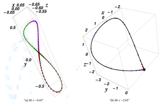
Combining Equations (11) and (12) we obtain four solutions of system (5) $(\pm x(t),$$\pm y\left(t\right),z\left(t\right))$ with ${\displaystyle \underset{t\to \pm \infty }{lim}(\pm x\left(t\right),\pm y\left(t\right),z\left(t\right))=(0,0,M)}$. Therefore, we obtain four homoclinic orbits, which are graphically depicted in Figure 1.

Figure 1. Equilibrium point $e_2^M(0,0,M)$ (black point) and the homoclinic orbits $\left(x\right(t),y(t),z(t\left)\right)$ (magenta), $\left(x\right(t),-y(t),z(t\left)\right)$ (red), $(-x(t),y(t),z(t\left)\right)$ (green), and $\left(x\right(t),y(t),z(t\left)\right)$ (blue) using Equations (11) and (12) for $M=5.15$, $a=0.5$, $b=0$, $c=0.75$, $d=-0.45$, $k=0.65$; initial data: $x_0=0.01$, $y_0=0.002$, $z_0=M$—exact solution (dotted color curve) and numerical results (solid black curve), respectively.

Related to the equilibrium point $e_1^M=\left(M,0,-{\displaystyle \frac{c}{d}}\right)$, when $-a(cM+d)\ne 0$, we assume that $a>0$ and $c<0$, $k>0$. Then, $i\sqrt{ck}\in \mathbb{R}$. The periodic orbit does not exists, but there exist heteroclinic orbits given by the intersection between the level sets $H_1(x,y,z)=H_1(M,0,-{\displaystyle \frac{d}{c}})$ and $C_1(x,y,z)=C_1(M,0,-{\displaystyle \frac{d}{c}})$ as follows:

$$\left\{\begin{array}{c}{\displaystyle \frac{k}{2}}{y}^2+{\displaystyle \frac{c}{2}}{\left(z+{\displaystyle \frac{d}{c}}\right)}^2=0\hfill \\ {\displaystyle \frac{ck}{2}}{x}^2+acz={\displaystyle \frac{ck}{2}}{M}^2-ad\hfill \end{array}\right..$$

(13)

The solution of the system (5) can be obtained by solving the previous system by

$$\left\{\begin{array}{c}x=\pm \sqrt{M^2-{\displaystyle \frac{2a}{k}}U}\hfill \\ y=\pm \sqrt{{\displaystyle \frac{-c}{k}}}U\hfill \\ z=U-{\displaystyle \frac{d}{c}}\hfill \end{array}\right..$$

(14)

Substituting Equation (14) into the first relation from Equation (5) yields the following differential equation

$$\pm {\displaystyle \frac{\dot{U}}{U\sqrt{M^2-\frac{2a}{k}U}}}=\mp \sqrt{-ck},$$

whose solution is

$$\begin{array}{c}\left|{\displaystyle \frac{V\left(t\right)+\left|M\right|}{V\left(t\right)-\left|M\right|}}\right|=e^{\pm \left|M\right|\sqrt{-ck}t+\mathcal{C}},\hfill \end{array}$$

(15)

where $V^2\left(t\right)=M^2-{\displaystyle \frac{2a}{k}}U\left(t\right)$. Then, we consider

$$\begin{array}{c}{V}_1\left(t\right)=\left|M\right|{\displaystyle \frac{1-e^{-p_1\left(t\right)}}{1+e^{-p_1\left(t\right)}}},V_2\left(t\right)=-\left|M\right|{\displaystyle \frac{1+e^{-p_1\left(t\right)}}{1-e^{-p_1\left(t\right)}}},\hfill \end{array}$$

(16)

where $p_1\left(t\right)=\left|M\right|\sqrt{-ck}t+\mathcal{C}$. Combining Equations (14) and (16), we obtain the following solutions of system (5)

$$\begin{array}{c}{x}_1\left(t\right)=V_1\left(t\right),y_1\left(t\right)={\displaystyle \frac{\sqrt{-ck}}{2a}}(V_1^2\left(t\right)-M^2),z_1\left(t\right)=-{\displaystyle \frac{d}{c}}-{\displaystyle \frac{k}{2a}}(V_1^2\left(t\right)-M^2),\hfill \\ x_2\left(t\right)=V_2\left(t\right),y_2\left(t\right)={\displaystyle \frac{\sqrt{-ck}}{2a}}(V_2^2\left(t\right)-M^2),z_2\left(t\right)=-{\displaystyle \frac{d}{c}}-{\displaystyle \frac{k}{2a}}(V_2^2\left(t\right)-M^2).\hfill \end{array}$$

(17)

These solutions yield four heteroclinic orbits as

$$(x_1\left(t\right),y_1\left(t\right),z_1\left(t\right)),(-x_1\left(t\right),y_1\left(t\right),z_1\left(t\right)),(x_1\left(t\right),-y_1\left(t\right),z_1\left(t\right)),(-x_1\left(t\right),-y_1\left(t\right),z_1\left(t\right)),$$

and four split-heteroclinic orbits as

$$(x_2\left(t\right),y_2\left(t\right),z_2\left(t\right)),(-x_2\left(t\right),y_2\left(t\right),z_2\left(t\right)),(x_2\left(t\right),-y_2\left(t\right),z_2\left(t\right)),(-x_2\left(t\right),-y_2\left(t\right),z_2\left(t\right)),$$

of system (5), respectively, with the following:

$$\begin{array}{c}{\displaystyle \underset{t\to \infty }{lim}(x_1\left(t\right),y_1\left(t\right),z_1\left(t\right))=\underset{t\to \infty }{lim}(x_1\left(t\right),-y_1\left(t\right),z_1\left(t\right))=(M,0,-\frac{d}{c}),}\hfill \\ {\displaystyle \underset{t\to -\infty }{lim}(-x_1\left(t\right),-y_1\left(t\right),z_1\left(t\right))=\underset{t\to -\infty }{lim}(-x_1\left(t\right),y_1\left(t\right),z_1\left(t\right))=(-M,0,-\frac{d}{c}),}\hfill \\ {\displaystyle \underset{t\to \infty }{lim}(x_2\left(t\right),y_2\left(t\right),z_2\left(t\right))=\underset{t\to \infty }{lim}(x_2\left(t\right),-y_2\left(t\right),z_2\left(t\right))=(M,0,-\frac{d}{c}),}\hfill \\ {\displaystyle \underset{t\to -\infty }{lim}(-x_2\left(t\right),-y_2\left(t\right),z_2\left(t\right))=\underset{t\to -\infty }{lim}(-x_2\left(t\right),y_2\left(t\right),z_2\left(t\right))=(-M,0,-\frac{d}{c}),}\hfill \end{array}$$

respectively.

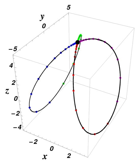
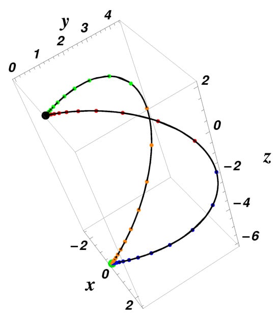
These eight heteroclinic orbits are graphically depicted in Figure 2.

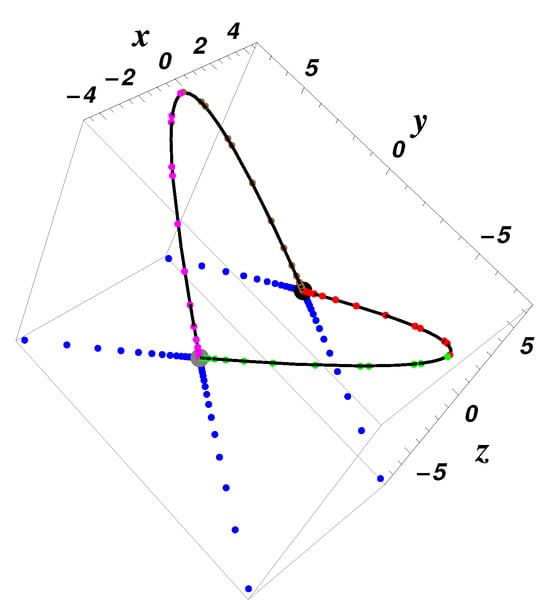
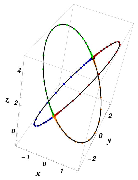
Figure 2. Equilibrium points $e_1^M(M,0,-d/c)$ (black point) and $e_1^{-M}(-M,0,-d/c)$ (green point); the heteroclinic orbits $(x_1\left(t\right),y_1\left(t\right),z_1\left(t\right))$ (red), $(-x_1\left(t\right),y_1\left(t\right),z_1\left(t\right))$ (green), $(x_1\left(t\right),-y_1\left(t\right),z_1\left(t\right))$ (brown), $(-x_1\left(t\right),-y_1\left(t\right),z_1\left(t\right))$ (magenta); and the split-heteroclinic orbits $(x_2\left(t\right),y_2\left(t\right),z_2\left(t\right))$, $(-x_2\left(t\right),y_2\left(t\right),z_2\left(t\right))$, $(x_2\left(t\right),-y_2\left(t\right),z_2\left(t\right))$, $(-x_2\left(t\right),-y_2\left(t\right),z_2\left(t\right))$ (blue), using Equations (16) and (17) for $M=3.25$, $a=0.5$, $b=0$, $c=-0.75$, $d=-0.45$, $k=0.65$; initial data: $x_0=3.24$, $y_0=0.001$, $z_0=-0.59$—exact solution (dotted color curve) and numerical results (solid black curve), respectively.

B. For $c=0$, the system (1) becomes as follows:

$$\left\{\begin{array}{c}\dot{x}=ay+byz\hfill \\ \dot{y}=dx\hfill \\ \dot{z}=-kxy\hfill \end{array}\right..$$

(18)

Then, the equilibrium points are $e_3^M=\left(0,M,-{\displaystyle \frac{a}{b}}\right)$, $M\ne 0$, and $e_4^M=\left(0,0,M\right)$.

The characteristic polynomial of $J\left(e_3^M\right)$ is

$$\begin{array}{c}{P}_{J\left(e_3^M\right)}\left(\lambda \right)=-\lambda \left({\lambda }^2+bk{M}^2\right),\hfill \end{array}$$

(19)

whose roots are

$$\begin{array}{c}{\lambda }_1=0,{\lambda }_{2,3}=\pm i\left|M\right|\sqrt{bk}\in \mathbb{C},\hfill \end{array}$$

(20)

for $bk>0$ (i.e., purely imaginary).

Therefore, there exists one periodic orbit of system (18) around the equilibrium point $e_3^M$ whose period is closed to ${\displaystyle \frac{2\pi }{\left|M\right|\sqrt{bk}}}$.

The characteristic polynomial of $J\left(e_4^M\right)$ is

$$\begin{array}{c}{P}_{J\left(e_4^M\right)}\left(\lambda \right)=-\lambda \left({\lambda }^2-d(a+bM)\right),\hfill \end{array}$$

(21)

whose roots are purely imaginary

$$\begin{array}{c}{\lambda }_1=0,{\lambda }_{2,3}=\pm i\sqrt{-d(a+bM)}\in \mathbb{C},\hfill \end{array}$$

(22)

for $-d(a+bM)>0$.

Therefore, there exists one periodic orbit of system (18) around the equilibrium point $e_4^M$ whose period is closed to ${\displaystyle \frac{2\pi }{\sqrt{-d(a+bM)}}}$.

Related to the equilibrium point $e_4^M=\left(0,0,M\right)$, when $-d(bM+a)<0$, we assume that $d<0$ and $bM+a<0$, $b>0$, $k>0$. Then, $i\sqrt{bk}\in \mathbb{C}$. The periodic orbit does not exists, but there exists homoclinic orbits given by the intersection between the level sets $H_1(x,y,z)=H_1(0,0,M)$ and $C_1(x,y,z)=C_1(0,0,M)$ as follows:

$$\left\{\begin{array}{c}{\displaystyle \frac{k}{b}}{x}^2+{\left(z+{\displaystyle \frac{a}{b}}\right)}^2={\left(M+{\displaystyle \frac{a}{b}}\right)}^2\hfill \\ {\displaystyle \frac{k}{2d}}{y}^2+z=M\hfill \end{array}\right..$$

(23)

The solution of system (18) can be obtained by using the following transformation

$$\left\{\begin{array}{c}x=\sqrt{{\displaystyle \frac{b}{k}}}\left(M+{\displaystyle \frac{a}{b}}\right){\displaystyle \frac{2U}{1+U^2}}\hfill \\ y=\pm \sqrt{{\displaystyle \frac{2}{k}}}\sqrt{(-d)(z-M)}\hfill \\ z=-{\displaystyle \frac{a}{b}}+\left(M+{\displaystyle \frac{a}{b}}\right){\displaystyle \frac{1-U^2}{1+U^2}}\hfill \end{array}\right..$$

(24)

Substituting Equation (24) into the second relation from Equation (18) yields the following differential equation

$${\displaystyle \frac{\dot{U}}{U\sqrt{1+U^2}}}=\pm \sqrt{d(bM+a)},$$

whose solution is

$$\begin{array}{c}U\left(t\right)=\pm {\displaystyle \frac{1}{sinh\left(\sqrt{d(bM+a)}t\right)}}.\hfill \end{array}$$

(25)

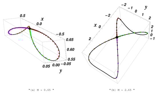
Combining Equations (24) and (25) we obtain four solutions of system (18) $(\pm x(t),\pm y(t),$$z\left(t\right))$ with ${\displaystyle \underset{t\to \pm \infty }{lim}(\pm x\left(t\right),\pm y\left(t\right),z\left(t\right))=(0,0,M)}$. Therefore, we obtain four homoclinic orbits which are graphically presented in Figure 3.

Figure 3. Equilibrium point $e_4^M(0,0,M)$ (black point) and the homoclinic orbits $\left(x\right(t),y(t),z(t\left)\right)$ (magenta), $(-x(t),y(t),z(t\left)\right)$ (red), $\left(x\right(t),-y(t),z(t\left)\right)$ (green), and $\left(x\right(t),y(t),z(t\left)\right)$ (blue), using Equations (24) and (25) for $M=-1.15$, $a=0.5$, $b=0.75$, $c=0$, $d=-0.45$, $k=0.65$; initial data: $x_0=0.01$, $y_0=0.02$, $z_0=M+0.01$—exact solution (dotted color curve) and numerical results (solid black curve), respectively.

Related to the equilibrium point $e_3^M=\left(0,M,-{\displaystyle \frac{a}{b}}\right)$, when $-d(bM+a)\ne 0$, we assume that $a>0$, $b<0$, $d<0$, $k>0$. Then, $i\sqrt{bk}\in \mathbb{R}$. The periodic orbit does not exists, but there exist heteroclinic orbits given by the intersection between the level sets $H_1(x,y,z)=H_1(0,M,-{\displaystyle \frac{a}{b}})$ and $C_1(x,y,z)=C_1(0,M,-{\displaystyle \frac{a}{b}})$ as follows:

$$\left\{\begin{array}{c}{\displaystyle \frac{k}{2}}{x}^2+{\displaystyle \frac{b}{2}}{\left(z+{\displaystyle \frac{a}{b}}\right)}^2=0\hfill \\ {\displaystyle \frac{-bk}{2}}{y}^2+(-b)dz={\displaystyle \frac{-bk}{2}}{M}^2+ad\hfill \end{array}\right..$$

(26)

The solution of system (18) can be obtained by solving the previous system by

$$\left\{\begin{array}{c}x=\pm \sqrt{{\displaystyle \frac{-b}{k}}}U\hfill \\ y=\pm \sqrt{M^2+{\displaystyle \frac{-2d}{k}}U}\hfill \\ z=U-{\displaystyle \frac{a}{b}}\hfill \end{array}\right..$$

(27)

Substituting Equation (27) into the third relation from Equation (18) yields the following differential equation

$$\pm {\displaystyle \frac{\dot{U}}{U\sqrt{M^2+\frac{-2d}{k}U}}}=\mp \sqrt{-bk},$$

whose solution is

$$\begin{array}{c}\left|{\displaystyle \frac{V\left(t\right)-\left|M\right|}{V\left(t\right)+\left|M\right|}}\right|=e^{\pm \left|M\right|\sqrt{-bk}t+\mathcal{C}},\hfill \end{array}$$

(28)

where $V^2\left(t\right)=M^2+{\displaystyle \frac{-2d}{k}}U\left(t\right)$. Then, we consider

$$\begin{array}{c}{V}_1\left(t\right)=\left|M\right|{\displaystyle \frac{1-e^{-p_3\left(t\right)}}{1+e^{-p_3\left(t\right)}}},V_2\left(t\right)=-\left|M\right|{\displaystyle \frac{1+e^{-p_3\left(t\right)}}{1-e^{-p_3\left(t\right)}}},\hfill \end{array}$$

(29)

where $p_3\left(t\right)=\left|M\right|\sqrt{-bk}t+\mathcal{C}$. Combining Equations (27) and (29), we obtain the following solutions of system (18)

$$\begin{array}{c}{x}_1\left(t\right)={\displaystyle \frac{\sqrt{-bk}}{-2d}}(V_1^2\left(t\right)-M^2),y_1\left(t\right)=V_1\left(t\right),z_1\left(t\right)=-{\displaystyle \frac{a}{b}}+{\displaystyle \frac{k}{-2d}}(V_1^2\left(t\right)-M^2),\hfill \\ x_2\left(t\right)={\displaystyle \frac{\sqrt{-bk}}{-2d}}(V_2^2\left(t\right)-M^2),y_2\left(t\right)=V_2\left(t\right),z_2\left(t\right)=-{\displaystyle \frac{a}{b}}+{\displaystyle \frac{k}{-2d}}(V_2^2\left(t\right)-M^2).\hfill \end{array}$$

(30)

These solutions yield four heteroclinic orbits of the system (18) as follows:

$$(x_1\left(t\right),y_1\left(t\right),z_1\left(t\right)),(-x_1\left(t\right),y_1\left(t\right),z_1\left(t\right)),(x_1\left(t\right),-y_1\left(t\right),z_1\left(t\right)),(-x_1\left(t\right),-y_1\left(t\right),z_1\left(t\right)),$$

and four split-heteroclinic orbits

$$(x_2\left(t\right),y_2\left(t\right),z_2\left(t\right)),(-x_2\left(t\right),y_2\left(t\right),z_2\left(t\right)),(x_2\left(t\right),-y_2\left(t\right),z_2\left(t\right)),(-x_2\left(t\right),-y_2\left(t\right),z_2\left(t\right)),$$

with the following:

$$\begin{array}{c}{\displaystyle \underset{t\to \infty }{lim}(x_1\left(t\right),y_1\left(t\right),z_1\left(t\right))=\underset{t\to \infty }{lim}(-x_1\left(t\right),y_1\left(t\right),z_1\left(t\right))=(0,M,-\frac{a}{b}),}\hfill \\ {\displaystyle \underset{t\to -\infty }{lim}(-x_1\left(t\right),-y_1\left(t\right),z_1\left(t\right))=\underset{t\to -\infty }{lim}(x_1\left(t\right),-y_1\left(t\right),z_1\left(t\right))=(0,-M,-\frac{a}{b}),}\hfill \\ {\displaystyle \underset{t\to \infty }{lim}(x_2\left(t\right),y_2\left(t\right),z_2\left(t\right))=\underset{t\to \infty }{lim}(-x_2\left(t\right),y_2\left(t\right),z_2\left(t\right))=(0,M,-\frac{a}{b}),}\hfill \\ {\displaystyle \underset{t\to -\infty }{lim}(-x_2\left(t\right),-y_2\left(t\right),z_2\left(t\right))=\underset{t\to -\infty }{lim}(x_2\left(t\right),-y_2\left(t\right),z_2\left(t\right))=(0,-M,-\frac{a}{b}),}\hfill \end{array}$$

respectively.

These eight heteroclinic orbits are graphically depicted in Figure 4.

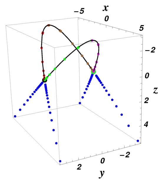
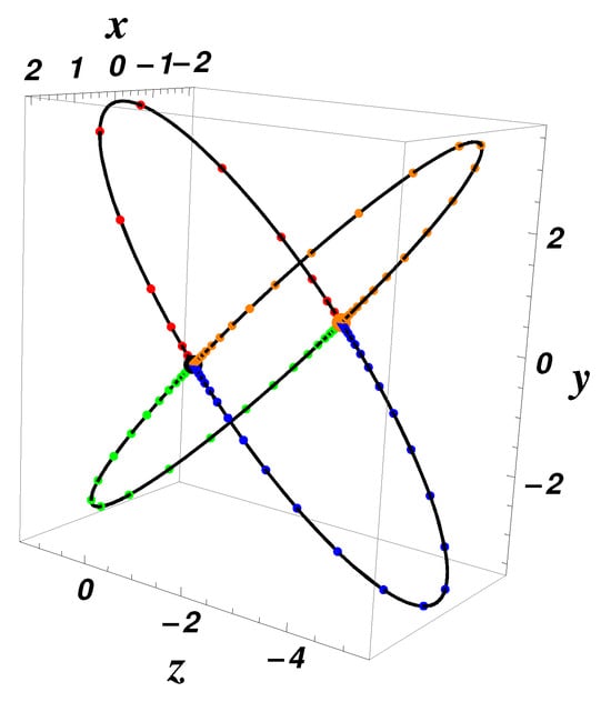
Figure 4. Equilibrium points $e_3^M(0,M,-a/b)$ (black point) and $e_3^{-M}(0,-M,-d/c)$ (green point); heteroclinic orbits $(x_1\left(t\right),y_1\left(t\right),z_1\left(t\right))$ (red), $(-x_1\left(t\right),y_1\left(t\right),z_1\left(t\right))$ (green), $(x_1\left(t\right),-y_1\left(t\right),z_1\left(t\right))$ (brown), $(-x_1\left(t\right),-y_1\left(t\right),z_1\left(t\right))$ (magenta); and split-heteroclinic orbits $(x_2\left(t\right),y_2\left(t\right),z_2\left(t\right))$, $(-x_2\left(t\right),y_2\left(t\right),z_2\left(t\right))$, $(x_2\left(t\right),-y_2\left(t\right),z_2\left(t\right))$, $(-x_2\left(t\right),-y_2\left(t\right),z_2\left(t\right))$ (blue), using Equations (29) and (30) for $M=2.25$, $a=0.5$, $b=-0.75$, $c=0$, $d=-0.45$, $k=0.65$; initial data: $x_0=0.001$, $y_0=M+0.001$, $z_0=-a/b-0.001$—exact solution (dotted color curve) and numerical results (solid black curve), respectively.

C. For $bc\ne 0$, the equilibrium points are $e_5^M=\left(0,M,-{\displaystyle \frac{a}{b}}\right)$, $M\ne 0$, $e_6^M=\left(M,0,-{\displaystyle \frac{d}{c}}\right)$, $M\ne 0$, and $e_7^M=\left(0,0,M\right)$.

The characteristic polynomial of $J\left(e_5^M\right)$ is

$$\begin{array}{c}{P}_{J\left(e_5^M\right)}\left(\lambda \right)=-\lambda \left({\lambda }^2+bk{M}^2\right),\hfill \end{array}$$

(31)

whose roots are

$$\begin{array}{c}{\lambda }_1=0,{\lambda }_{2,3}=\pm i\left|M\right|\sqrt{bk}\in \mathbb{C},\hfill \end{array}$$

(32)

for $bk>0$ (i.e., purely imaginary).

Therefore, there exists one periodic orbit of system (1) around the equilibrium point $e_5^M$ whose period is closed to ${\displaystyle \frac{2\pi }{\left|M\right|\sqrt{bk}}}$.

The characteristic polynomial of $J\left(e_6^M\right)$ is

$$\begin{array}{c}{P}_{J\left(e_6^M\right)}\left(\lambda \right)=-\lambda \left({\lambda }^2+ck{M}^2\right),\hfill \end{array}$$

(33)

whose roots are purely imaginary

$$\begin{array}{c}{\lambda }_1=0,{\lambda }_{2,3}=\pm i\left|M\right|\sqrt{ck}\in \mathbb{C},\hfill \end{array}$$

(34)

for $ck>0$.

Therefore, there exists one periodic orbit of system (1) around the equilibrium point $e^M$ whose period is closed to ${\displaystyle \frac{2\pi }{\left|M\right|\sqrt{ck}}}$.

The characteristic polynomial of $J\left(e_7^M\right)$ is

$$\begin{array}{c}{P}_{J\left(e_7^M\right)}\left(\lambda \right)=-\lambda \left({\lambda }^2-(a+bM)(cM+d)\right),\hfill \end{array}$$

(35)

whose roots are purely imaginary

$$\begin{array}{c}{\lambda }_1=0,{\lambda }_{2,3}=\pm i\sqrt{-(a+bM)(cM+d)}\in \mathbb{C},\hfill \end{array}$$

(36)

for $-(a+bM)(cM+d)>0$.

Therefore, there exists one periodic orbit of system (1) around the equilibrium point $e_7^M$ whose period is closed to ${\displaystyle \frac{2\pi }{\sqrt{-(a+bM)(cM+d)}}}$.

In the case $ac-bd>0$ with $bc>0$, the condition $-(a+bM)(cM+d)>0$ is true if and only if $M\in \left(-{\displaystyle \frac{a}{b}},-{\displaystyle \frac{d}{c}}\right)\cup \left(-{\displaystyle \frac{d}{c}},-{\displaystyle \frac{a}{b}}\right)$.

In the case $ac-bd>0$ with $bc<0$, the condition $-(a+bM)(cM+d)>0$ is true if and only if $M\in \left(-\infty ,-{\displaystyle \frac{a}{b}}\right)\cup \left(-{\displaystyle \frac{d}{c}},\infty \right)$ or $M\in \left(-\infty ,-{\displaystyle \frac{d}{c}}\right)\cup \left(-{\displaystyle \frac{a}{b}},\infty \right)$.

The case $ac-bd<0$ is similar to the case $ad-bc>0$.

In relation to the equilibrium point $e_7^M=\left(0,0,M\right)$, when $-(bM+a)(cM+d)<0$, we assume that $d<0$, $b>0$, $c>0$ and $k>0$. Then, $i\sqrt{-(bM+a)(cM+d)}\in \mathbb{R}$. The periodic orbit does not exist, but there exists homoclinic orbits given by the intersection between the level sets $H_1(x,y,z)=H_1(0,0,M)$ and $C_1(x,y,z)=C_1(0,0,M)$ as follows:

$$\left\{\begin{array}{c}{\displaystyle \frac{k}{b}}{x}^2+{\left(z+{\displaystyle \frac{a}{b}}\right)}^2={\left(M+{\displaystyle \frac{a}{b}}\right)}^2\hfill \\ {\displaystyle \frac{k}{c}}{y}^2+{\left(z+{\displaystyle \frac{d}{c}}\right)}^2={\left(M+{\displaystyle \frac{d}{c}}\right)}^2\hfill \end{array}\right..$$

(37)

The solution of system (1) can be obtained by using the following transformation

$$\left\{\begin{array}{c}x=\pm \sqrt{{\displaystyle \frac{b}{k}}}\sqrt{{\left(M+{\displaystyle \frac{a}{b}}\right)}^2-{\left(z+{\displaystyle \frac{a}{b}}\right)}^2}\hfill \\ y=\pm \sqrt{{\displaystyle \frac{c}{k}}}\sqrt{{\left(M+{\displaystyle \frac{d}{c}}\right)}^2-{\left(z+{\displaystyle \frac{d}{c}}\right)}^2}\hfill \\ z=|{\displaystyle \frac{a}{b}}-{\displaystyle \frac{d}{c}}|{\displaystyle \frac{1+U^2}{2U}}-M-\left({\displaystyle \frac{a}{b}}+{\displaystyle \frac{d}{c}}\right)\hfill \end{array}\right..$$

(38)

Substituting Equation (38) into the third relation from Equation (1) yields the following differential equation

$${\displaystyle \frac{2\dot{U}}{2U\left(2M+\frac{a}{b}+\frac{d}{c}\right)-\left(\frac{a}{b}-\frac{d}{c}\right)(1+U^2)}}=\pm \sqrt{bc},$$

whose solutions are

$$\begin{array}{c}{U}_1\left(t\right)=A_0+B_0{\displaystyle \frac{1-e^{-p_7\left(t\right)}}{1+e^{-p_7\left(t\right)}}},U_2\left(t\right)=A_0+B_0{\displaystyle \frac{1+e^{-p_7\left(t\right)}}{1-e^{-p_7\left(t\right)}}},\hfill \end{array}$$

(39)

where $p_7\left(t\right)=2\sqrt{(bM+a)(cM+d)}t+\mathcal{C}$, $A_0={\displaystyle \frac{2M+\frac{a}{b}+\frac{d}{c}}{|\frac{a}{b}-\frac{d}{c}|}}$, $B_0=2{\displaystyle \frac{\sqrt{\left(M+\frac{a}{b}\right)\left(M+\frac{d}{c}\right)}}{|\frac{a}{b}-\frac{d}{c}|}}$.

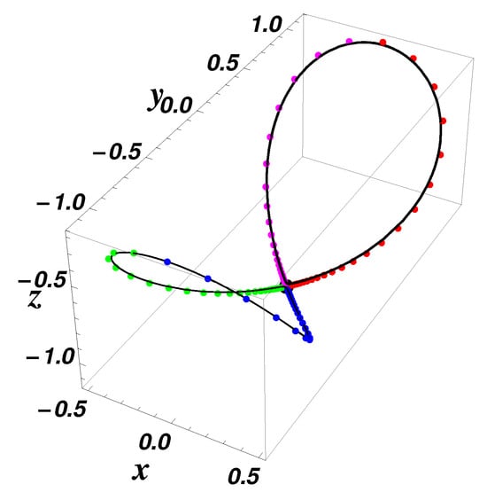
Combining Equations (38) and (39), for $U_1\left(t\right)$, we obtain four solutions of system (1) $(x_1\left(t\right),y_1\left(t\right),z_1\left(t\right))$, $(-x_1\left(t\right),-y_1\left(t\right),z_1\left(t\right))$, $(-x_1\left(t\right),y_1\left(t\right),z_1\left(t\right))$, $(x_1\left(t\right),-y_1\left(t\right),z_1\left(t\right))$ for $M>-d/c$ and $M<-1$, respectively, and two solutions of system (1) $(-x_1\left(t\right),-y_1\left(t\right),z_1\left(t\right))$, $(x_1\left(t\right),-y_1\left(t\right),z_1\left(t\right))$, for $-1<M<-a/b$ with ${\displaystyle \underset{t\to \pm \infty }{lim}(\pm x_1\left(t\right),\pm y_1\left(t\right),z_1\left(t\right))=(0,0,M)}$. These homoclinic orbits are graphically shown in Figure 5 and Figure 6, respectively.

Figure 5. Equilibrium point $e_7^M(0,0,M)$ (black point) and the homoclinic orbits $(x_i\left(t\right),y_i\left(t\right),z_i\left(t\right))$, $i=1,2$, using Equations (38) and (39) for $a=0.5$, $b=0.85$, $c=0.75$, $d=-0.45$, $k=0.65$; initial data: $x_0=-0.001$, $y_0=-0.002$, $z_0=M+0.001$—exact solution (dotted color curve) and numerical results (solid black curve), respectively: (a) $M=-0.65$; (b) $M=-2.65$.

Figure 6. Equilibrium point $e_7^M(0,0,M)$ (black point) and the homoclinic orbits $(x_i\left(t\right),y_i\left(t\right),z_i\left(t\right))$, $i=1,2$, using Equations (38) and (39) for $a=0.5$, $b=0.85$, $c=0.75$, $d=-0.45$, $k=0.65$; initial data: $x_0=-0.001$, $y_0=-0.002$, $z_0=M+0.001$—exact solution (dotted color curve) and numerical results (solid black curve), respectively. (a) $M=-0.65$; (b) $M=-2.65$.

2.2. Case 2— $ac-bd=0$

The system (1) becomes as follows:

$$\left\{\begin{array}{c}\dot{x}=ay+byz\hfill \\ \dot{y}=cxz+{\displaystyle \frac{ac}{b}}x\hfill \\ \dot{z}=-kxy\hfill \end{array}\right.,b\ne 0.$$

(40)

In this case, the Hamiltonian $H_2$ and the Casimir $C_2$ of the system (40) are

$$\left\{\begin{array}{c}{H}_2(x,y,z)={\displaystyle \frac{k}{2}}{x}^2+{\displaystyle \frac{b}{2}}{\left(z+{\displaystyle \frac{a}{b}}\right)}^2\hfill \\ C_2(x,y,z)={\displaystyle \frac{c}{2}}{x}^2-{\displaystyle \frac{b}{2}}{y}^2\hfill \end{array}\right..$$

(41)

By means of these prime integrals (constants of motion), the semi-analytical solutions in closed-form could be obtained using the OAFM procedure [23]. This solution will be called the OAFM-solution and is denoted by $\overline{u}$ or ${\overline{u}}_{OAFM}$. The accuracy is validated in Section 4.2.

For $ac-bd=0$, the system (40) admits symmetries with respect to the Oz-axis, being invariant to transformation $(x,y,z)\to (-x,-y,z)$.

Assume that $d={\displaystyle \frac{ac}{b}}$. Then, the equilibrium points are as follows: $e_8^M=\left(0,M,-{\displaystyle \frac{a}{b}}\right)$, $M\ne 0$, $e_9^M=\left(M,0,-{\displaystyle \frac{a}{b}}\right)$, $M\ne 0$, and $e_{10}^M=\left(0,0,M\right)$.

The characteristic polynomial of $J\left(e_8^M\right)$ is

$$\begin{array}{c}{P}_{J\left(e_8^M\right)}\left(\lambda \right)=-\lambda \left({\lambda }^2+bk{M}^2\right),\hfill \end{array}$$

(42)

whose roots are

$$\begin{array}{c}{\lambda }_1=0,{\lambda }_{2,3}=\pm i\left|M\right|\sqrt{bk}\in \mathbb{C},\hfill \end{array}$$

(43)

for $bk>0$ (i.e., purely imaginary).

Therefore, there exists one periodic orbit of system (40) around the equilibrium point $e_8^M$ whose period is closed to ${\displaystyle \frac{2\pi }{\left|M\right|\sqrt{bk}}}$.

The characteristic polynomial of $J\left(e_9^M\right)$ is

$$\begin{array}{c}{P}_{J\left(e_9^M\right)}\left(\lambda \right)=-\lambda \left({\lambda }^2+ck{M}^2\right),\hfill \end{array}$$

(44)

whose roots are purely imaginary

$$\begin{array}{c}{\lambda }_1=0,{\lambda }_{2,3}=\pm i\left|M\right|\sqrt{ck}\in \mathbb{C},\hfill \end{array}$$

(45)

for $ck>0$.

Therefore, there exists one periodic orbit of system (40) around the equilibrium point $e_9^M$ whose period is closed to ${\displaystyle \frac{2\pi }{\left|M\right|\sqrt{ck}}}$.

The characteristic polynomial of $J\left(e_{10}^M\right)$ is

$$\begin{array}{c}{P}_{J\left(e_{10}^M\right)}\left(\lambda \right)=-\lambda \left({\lambda }^2-{\displaystyle \frac{c}{b}}{(a+bM)}^2\right),\hfill \end{array}$$

(46)

whose roots are purely imaginary

$$\begin{array}{c}{\lambda }_1=0,{\lambda }_{2,3}=\pm i|a+bM|\sqrt{-{\displaystyle \frac{c}{b}}}\in \mathbb{C},\hfill \end{array}$$

(47)

for $-{\displaystyle \frac{c}{b}}>0$ and $M\ne -{\displaystyle \frac{a}{b}}$.

Therefore, there exists one periodic orbit of system (40) around the equilibrium point $e_{10}^M$ whose period is closed to ${\displaystyle \frac{2\pi }{|a+bM|\sqrt{-\frac{c}{b}}}}$.

Related to the equilibrium point $e_8^M=\left(0,M,-a/b\right)$, when $b<0$, we assume that $a>0$, $c>0$, and $k>0$. Then, $i\sqrt{-bk}\in \mathbb{C}$. The periodic orbit does not exist, but there exist eight heteroclinic orbits given by the intersection between the level sets $H_2(x,y,z)=H_2(0,M,-a/b)$ and $C_2(x,y,z)=C_2(0,M,-a/b)$ as follows:

$$\left\{\begin{array}{c}{\displaystyle \frac{k}{2}}{x}^2-{\displaystyle \frac{-b}{2}}{\left(z+{\displaystyle \frac{a}{b}}\right)}^2=0\hfill \\ {\displaystyle \frac{c}{2}}{x}^2-{\displaystyle \frac{b}{2}}{y}^2=-{\displaystyle \frac{b}{2}}{M}^2\hfill \end{array}\right..$$

(48)

The solution of the system (40) can be obtained by solving the previous system by

$$\left\{\begin{array}{c}x=\pm \sqrt{{\displaystyle \frac{-b}{c}}}M{\displaystyle \frac{1-U^2}{1+U^2}}\hfill \\ y=\pm M{\displaystyle \frac{2U}{1+U^2}}\hfill \\ z=-{\displaystyle \frac{a}{b}}+\sqrt{{\displaystyle \frac{k}{c}}}M{\displaystyle \frac{1-U^2}{1+U^2}}\hfill \end{array}\right..$$

(49)

Substituting Equation (49) into the third relation from Equation (40) yields the following differential equation

$${\displaystyle \frac{2\dot{U}}{U^2-1}}=\pm \sqrt{-bk}M,$$

whose solutions are

$$\begin{array}{c}{U}_1\left(t\right)={\displaystyle \frac{1-\mathcal{C}{e}^{-p_8\left(t\right)}}{1+\mathcal{C}{e}^{-p_8\left(t\right)}}},U_2\left(t\right)={\displaystyle \frac{1+\mathcal{C}{e}^{-p_8\left(t\right)}}{1-\mathcal{C}{e}^{-p_8\left(t\right)}}},\hfill \end{array}$$

(50)

where $p_8\left(t\right)=\sqrt{-bk}Mt$, $\mathcal{C}=\left|{\displaystyle \frac{1-U\left(0\right)}{1+U\left(0\right)}}\right|$, and $U\left(0\right)=-\sqrt{{\displaystyle \frac{z\left(0\right)+\frac{a}{b}+M\sqrt{\frac{k}{c}}}{M\sqrt{\frac{k}{c}}-z\left(0\right)-\frac{a}{b}}}}$. Combining Equations (49) and (50), we obtain the following solutions of system (40)

$$\begin{array}{c}{x}_1\left(t\right)=\sqrt{{\displaystyle \frac{-b}{c}}}M{\displaystyle \frac{1-U_1^2}{1+U_1^2}},y_1\left(t\right)=M{\displaystyle \frac{2U_1}{1+U_1^2}},z_1\left(t\right)=-{\displaystyle \frac{a}{b}}+\sqrt{{\displaystyle \frac{k}{c}}}M{\displaystyle \frac{1-U_1^2}{1+U_1^2}},\hfill \\ x_2\left(t\right)=\sqrt{{\displaystyle \frac{-b}{c}}}M{\displaystyle \frac{1-U_2^2}{1+U_2^2}},y_2\left(t\right)=M{\displaystyle \frac{2U_2}{1+U_2^2}},z_2\left(t\right)=-{\displaystyle \frac{a}{b}}+\sqrt{{\displaystyle \frac{k}{c}}}M{\displaystyle \frac{1-U_2^2}{1+U_2^2}}.\hfill \end{array}$$

(51)

These solutions describe only four heteroclinic orbits of the system (40) as follows:

$$(x_1\left(t\right),y_1\left(t\right),z_1\left(t\right)),(-x_1\left(t\right),y_1\left(t\right),z_1\left(t\right)),(x_2\left(t\right),y_2\left(t\right),z_2\left(t\right)),(-x_2\left(t\right),y_2\left(t\right),z_2\left(t\right)),$$

with

$${\displaystyle \underset{t\to \infty }{lim}(x_1\left(t\right),y_1\left(t\right),z_1\left(t\right))=\underset{t\to \infty }{lim}(-x_1\left(t\right),y_1\left(t\right),z_1\left(t\right))=(0,M,-a/b),}$$

$$\underset{t\to \infty }{lim}(x_2\left(t\right),y_2\left(t\right),z_2\left(t\right))=\underset{t\to \infty }{lim}(-x_2\left(t\right),y_2\left(t\right),z_2\left(t\right))=(0,M,-a/b),$$

$${\displaystyle \underset{t\to -\infty }{lim}(x_1\left(t\right),y_1\left(t\right),z_1\left(t\right))=\underset{t\to -\infty }{lim}(-x_1\left(t\right),y_1\left(t\right),z_1\left(t\right))=(0,-M,-a/b),}$$

$$\underset{t\to -\infty }{lim}(x_2\left(t\right),y_2\left(t\right),z_2\left(t\right))=\underset{t\to -\infty }{lim}(-x_2\left(t\right),y_2\left(t\right),z_2\left(t\right))=(0,-M,-a/b).$$

Therefore, we obtain only four heteroclinic orbits which are graphically depicted in Figure 7.

Figure 7. Equilibrium points $e_8^M(0,M,-a/b)$ (black point) and $e_8^{-M}(0,-M,-a/b)$ (orange point) and the heteroclinic orbits $(x_1\left(t\right),y_1\left(t\right),z_1\left(t\right))$ (red), $(-x_1\left(t\right),y_1\left(t\right),z_1\left(t\right))$ (green), $(x_2\left(t\right),y_2\left(t\right),z_2\left(t\right))$ (blue), $(-x_2\left(t\right),y_2\left(t\right),z_2\left(t\right))$ (orange) using Equations (50) and (51) for $M=2.05$, $a=0.5$, $b=-0.25$, $c=0.75$, $d={\displaystyle \frac{ac}{b}}$, $k=0.65$; initial data: $x_0=0.002$, $y_0=M+0.001$, $z_0=-a/b+0.001$—exact solution (dotted color curve) and numerical results (solid black curve), respectively.

Related to the equilibrium point $e_9^M=\left(M,0,-a/b\right)$, when $c<0$, we assume that $a>0$ and $b>0$, $k>0$. Then, $i\sqrt{-ck}\in \mathbb{C}$. The periodic orbit does not exist, but there exist two heteroclinic orbits given by the intersection between the level sets $H_2(x,y,z)=H_2(M,0,-a/b)$ and $C_2(x,y,z)=C_2(M,0,-a/b)$ as follows:

$$\left\{\begin{array}{c}{\displaystyle \frac{k}{2}}{x}^2+{\displaystyle \frac{b}{2}}{\left(z+{\displaystyle \frac{a}{b}}\right)}^2={\displaystyle \frac{b}{2}}{M}^2\hfill \\ {\displaystyle \frac{c}{2}}{x}^2-{\displaystyle \frac{b}{2}}{y}^2={\displaystyle \frac{c}{2}}{M}^2\hfill \end{array}\right..$$

(52)

The solution of the system (40) can be obtained by solving the previous system by

$$\left\{\begin{array}{c}x=\pm M{\displaystyle \frac{2U}{1+U^2}}\hfill \\ y=\pm \sqrt{{\displaystyle \frac{-c}{b}}}M{\displaystyle \frac{1-U^2}{1+U^2}}\hfill \\ z=-{\displaystyle \frac{a}{b}}+\sqrt{{\displaystyle \frac{k}{b}}}M{\displaystyle \frac{1-U^2}{1+U^2}}\hfill \end{array}\right..$$

(53)

Substituting Equation (53) into the first relation from Equation (40) yields the following differential equation

$${\displaystyle \frac{2\dot{U}}{U^2-1}}=\pm \sqrt{-ck}M,$$

whose solutions are

$$\begin{array}{c}{U}_1\left(t\right)={\displaystyle \frac{1-\mathcal{C}{e}^{-p_9\left(t\right)}}{1+\mathcal{C}{e}^{-p_9\left(t\right)}}},U_2\left(t\right)={\displaystyle \frac{1+\mathcal{C}{e}^{-p_9\left(t\right)}}{1-\mathcal{C}{e}^{-p_9\left(t\right)}}},\hfill \end{array}$$

(54)

where $p_9\left(t\right)=\sqrt{-ck}Mt$, $\mathcal{C}=\left|{\displaystyle \frac{1-U\left(0\right)}{1+U\left(0\right)}}\right|$, and $U\left(0\right)=-\sqrt{{\displaystyle \frac{z\left(0\right)+\frac{a}{b}+M\sqrt{\frac{k}{b}}}{M\sqrt{\frac{k}{b}}-z\left(0\right)-\frac{a}{b}}}}$.

Combining Equations (53) and (54), we obtain the following solutions of system (40)

$$\begin{array}{c}{x}_1\left(t\right)=M{\displaystyle \frac{2U_1}{1+U_1^2}},y_1\left(t\right)=\sqrt{{\displaystyle \frac{-c}{b}}}M{\displaystyle \frac{1-U_1^2}{1+U_1^2}},z_1\left(t\right)=-{\displaystyle \frac{a}{b}}+\sqrt{{\displaystyle \frac{k}{b}}}M{\displaystyle \frac{1-U_1^2}{1+U_1^2}},\hfill \\ x_2\left(t\right)=M{\displaystyle \frac{2U_2}{1+U_2^2}},y_2\left(t\right)=\sqrt{{\displaystyle \frac{-c}{b}}}M{\displaystyle \frac{1-U_2^2}{1+U_2^2}},z_2\left(t\right)=-{\displaystyle \frac{a}{b}}+\sqrt{{\displaystyle \frac{k}{b}}}M{\displaystyle \frac{1-U_2^2}{1+U_2^2}}.\hfill \end{array}$$

(55)

These solutions describe only four heteroclinic orbits of the system (40) as follows:

$$(x_1\left(t\right),y_1\left(t\right),z_1\left(t\right)),(x_1\left(t\right),-y_1\left(t\right),z_1\left(t\right)),(x_2\left(t\right),y_2\left(t\right),z_2\left(t\right)),(x_2\left(t\right),-y_2\left(t\right),z_2\left(t\right)),$$

with

$${\displaystyle \underset{t\to \infty }{lim}(x_1\left(t\right),y_1\left(t\right),z_1\left(t\right))=\underset{t\to \infty }{lim}(x_1\left(t\right),-y_1\left(t\right),z_1\left(t\right))=(M,0,-a/b),}$$

$$\underset{t\to \infty }{lim}(x_2\left(t\right),y_2\left(t\right),z_2\left(t\right))=\underset{t\to \infty }{lim}(x_2\left(t\right),-y_2\left(t\right),z_2\left(t\right))=(M,0,-a/b),$$

$${\displaystyle \underset{t\to -\infty }{lim}(x_1\left(t\right),y_1\left(t\right),z_1\left(t\right))=\underset{t\to -\infty }{lim}(x_1\left(t\right),-y_1\left(t\right),z_1\left(t\right))=(-M,0,-a/b),}$$

$$\underset{t\to -\infty }{lim}(x_2\left(t\right),y_2\left(t\right),z_2\left(t\right))=\underset{t\to -\infty }{lim}(x_2\left(t\right),-y_2\left(t\right),z_2\left(t\right))=(-M,0,-a/b).$$

Therefore, we obtain only four heteroclinic orbits, which are graphically depicted in Figure 8.

Figure 8. Equilibrium points $e_9^M(M,0,-a/b)$ (black point) and $e_9^{-M}(-M,0,-a/b)$ (orange point) and the heteroclinic orbits $(x_1\left(t\right),y_1\left(t\right),z_1\left(t\right))$ (red), $(x_1\left(t\right),-y_1\left(t\right),z_1\left(t\right))$ (green), $(x_2\left(t\right),y_2\left(t\right),z_2\left(t\right))$ (blue), $(x_2\left(t\right),-y_2\left(t\right),z_2\left(t\right))$ (orange), using Equations (54) and (55) for $M=2.05$, $a=0.5$, $b=0.25$, $c=-0.75$, $d={\displaystyle \frac{ac}{b}}$, $k=0.65$; initial data: $x_0=M+0.001$, $y_0=0.002$, $z_0=-a/b+0.001$—exact solution (dotted color curve) and numerical results (solid black curve), respectively.

Related to the equilibrium point $e_{10}^M=\left(0,0,M\right)$, when $bM+a\ne 0$ and $-c/b<0$, we assume that $a>0$ and $b>0$, $c>0$, $k>0$. Then, $i\sqrt{-c/b}\in \mathbb{R}$. The periodic orbit does not exist, but there exist four heteroclinic orbits given by the intersection between the level sets $H_2(x,y,z)=H_2(0,0,M)$ and $C_2(x,y,z)=C_2(0,0,M)$ as follows:

$$\left\{\begin{array}{c}{\displaystyle \frac{k}{2}}{x}^2+{\displaystyle \frac{b}{2}}{\left(z+{\displaystyle \frac{a}{b}}\right)}^2={\displaystyle \frac{b}{2}}{\left(M+{\displaystyle \frac{a}{b}}\right)}^2\hfill \\ {\displaystyle \frac{c}{2}}{x}^2-{\displaystyle \frac{b}{2}}{y}^2=0\hfill \end{array}\right..$$

(56)

The solution of the system (40) can be obtained by solving the previous system by

$$\left\{\begin{array}{c}x=\pm \sqrt{{\displaystyle \frac{b}{k}}}\left(M+{\displaystyle \frac{a}{b}}\right){\displaystyle \frac{2U}{1+U^2}}\hfill \\ y=\pm \sqrt{{\displaystyle \frac{c}{b}}}x\hfill \\ z=-{\displaystyle \frac{a}{b}}+\left(M+{\displaystyle \frac{a}{b}}\right){\displaystyle \frac{1-U^2}{1+U^2}}\hfill \end{array}\right..$$

(57)

Substituting Equation (57) into the first relation from Equation (40) yields the following differential equation

$${\displaystyle \frac{\dot{U}}{U}}=\pm \sqrt{bc}\left(M+{\displaystyle \frac{a}{b}}\right),$$

whose solutions are

$$\begin{array}{c}{U}_1\left(t\right)=e^{-p_{10}\left(t\right)},U_2\left(t\right)=e^{p_{10}\left(t\right)},\hfill \end{array}$$

(58)

where $p_{10}\left(t\right)=\sqrt{bc}\left(M+{\displaystyle \frac{a}{b}}\right)t+\mathcal{C}$. Combining Equations (57) and (58), we obtain the following solutions of system (40)

$$\begin{array}{c}{x}_1\left(t\right)=\sqrt{{\displaystyle \frac{b}{k}}}\left(M+{\displaystyle \frac{a}{b}}\right){\displaystyle \frac{2U_1}{1+U_1^2}},x_2\left(t\right)=\sqrt{{\displaystyle \frac{b}{k}}}\left(M+{\displaystyle \frac{a}{b}}\right){\displaystyle \frac{2U_2}{1+U_2^2}},\hfill \\ y_1\left(t\right)=\sqrt{{\displaystyle \frac{c}{b}}}{x}_1,y_2\left(t\right)=\sqrt{{\displaystyle \frac{c}{b}}}{x}_2,\hfill \\ z_1\left(t\right)=-{\displaystyle \frac{a}{b}}+\left(M+{\displaystyle \frac{a}{b}}\right){\displaystyle \frac{1-U_1^2}{1+U_1^2}},z_2\left(t\right)=-{\displaystyle \frac{a}{b}}+\left(M+{\displaystyle \frac{a}{b}}\right){\displaystyle \frac{1-U_2^2}{1+U_2^2}}.\hfill \end{array}$$

(59)

These solutions describe four heteroclinic orbits of the system (40) as follows:

$$(x_1\left(t\right),y_1\left(t\right),z_1\left(t\right)),(-x_1\left(t\right),y_1\left(t\right),z_1\left(t\right)),(x_2\left(t\right),y_2\left(t\right),z_2\left(t\right)),(-x_2\left(t\right),y_2\left(t\right),z_2\left(t\right)),$$

with

$${\displaystyle \underset{t\to \infty }{lim}(x_1\left(t\right),y_1\left(t\right),z_1\left(t\right))=\underset{t\to \infty }{lim}(-x_1\left(t\right),y_1\left(t\right),z_1\left(t\right))=(0,0,M),}$$

$${\displaystyle \underset{t\to -\infty }{lim}(x_2\left(t\right),y_2\left(t\right),z_2\left(t\right))=\underset{t\to -\infty }{lim}(-x_2\left(t\right),y_2\left(t\right),z_2\left(t\right))=(0,0,-M-\frac{2a}{b}).}$$

Therefore, we obtain four heteroclinic orbits, which are graphically depicted in Figure 9.

Figure 9. Equilibrium points $e_{10}^M(0,0,M)$ (black point) and $e_{10}^{-M-2a/b}(0,0,-M-{\displaystyle \frac{2a}{b}})$ (green point) and the heteroclinic orbits $(x_1\left(t\right),y_1\left(t\right),z_1\left(t\right))$ (red), $(-x_1\left(t\right),y_1\left(t\right),z_1\left(t\right))$ (green), $(x_2\left(t\right),y_2\left(t\right),z_2\left(t\right))$ (blue), $(-x_2\left(t\right),y_2\left(t\right),z_2\left(t\right))$ (orange), using Equations (58) and (59) for $M=2.05$, $a=0.5$, $b=0.25$, $c=0.75$, $d={\displaystyle \frac{ac}{b}}$, $k=0.65$; initial data: $x_0=0.001$, $y_0=0.002$, $z_0=M+0.001$—exact solution (dotted color curve) and numerical results (solid black curve), respectively.

Remark 1.

For $b<0$, $c<0$, and $d={\displaystyle \frac{ac}{b}}$, the system (40) admits periodic solutions if and only if $k<0$.

Remark 2.

All the analyzed cases lead to the periodic behaviors of the system described by Equation (1). The periodic solutions will be numerically computed in Section 4.2 using the OAFM technique for several values of the physical parameters a, b, c, d, $k>0$ and initial conditions $x_0>0$, $y_0>0$, $z_0>0$, respectively.

3. Closed-Form Solutions

In this section, closed-form solutions for the system (1) are obtained using the prime integrals presented in the previous section for each relevant case for our study.

In the case, $ac-bd\ne 0$, $c>0$, $k>0$ with $b=0$, considering the second prime integral (3) for $z\left(t\right)$ and the first equation from (5) for $y\left(t\right)$.

The closed-form solutions are written as

$$\left\{\begin{array}{c}x=u\hfill \\ y={\displaystyle \frac{1}{a}}\dot{u}\hfill \\ z=-{\displaystyle \frac{k}{2a}}{u}^2+\left(z_0+{\displaystyle \frac{k}{2a}}{x}_0^2\right)\hfill \end{array}\right.,$$

(60)

where the unknown smooth function $u\left(t\right)$ is the solution of the following problem

$$\left\{\begin{array}{c}{\displaystyle \frac{1}{a}}\ddot{u}+{\displaystyle \frac{ck}{2a}}{u}^3-c\left(z_0+{\displaystyle \frac{k}{2a}}{x}_0^2\right)u-du=0\hfill \\ u\left(0\right)=x_0,\dot{u}\left(0\right)=a{y}_0\hfill \end{array}\right..$$

(61)

Considering $ac-bd\ne 0$, $b>0$, $k>0$ for $c=0$ and taking into account the second prime integral (3) for $z\left(t\right)$, respectively, the second equation from (18) for $x\left(t\right)$, the closed-form solutions are written as

$$\left\{\begin{array}{c}x={\displaystyle \frac{1}{d}}\dot{u}\hfill \\ y=u\hfill \\ z=-{\displaystyle \frac{k}{2d}}{u}^2+\left(z_0+{\displaystyle \frac{k}{2d}}{y}_0^2\right)\hfill \end{array}\right.,$$

(62)

where the unknown smooth function $u\left(t\right)$ is the solution of the following problem

$$\left\{\begin{array}{c}{\displaystyle \frac{1}{d}}\ddot{u}+{\displaystyle \frac{bk}{2d}}{u}^3-b\left(z_0+{\displaystyle \frac{k}{2d}}{y}_0^2\right)u-au=0\hfill \\ u\left(0\right)=y_0,\dot{u}\left(0\right)=d{x}_0\hfill \end{array}\right..$$

(63)

In the case $ac-bd\ne 0$, $k>0$, $b>0$ and $c>0$, but $a<0$ and $d<0$, using the second prime integral (3) for $y\left(t\right),z\left(t\right)$, respectively, the last equation from (1) for $x\left(t\right)$, the closed-form solutions are defined by the following:

$$\left\{\begin{array}{c}x={\displaystyle \frac{1}{\sqrt{ck}}}{\displaystyle \frac{2\dot{u}}{1+u^2}}\hfill \\ y={\displaystyle \frac{R}{\sqrt{k}}}{\displaystyle \frac{2u}{1+u^2}}\hfill \\ z=-{\displaystyle \frac{d}{c}}+{\displaystyle \frac{R}{\sqrt{c}}}{\displaystyle \frac{1-u^2}{1+u^2}}\hfill \end{array}\right.,$$

(64)

where the unknown smooth function $u\left(t\right)$ is the solution of the following problem

$$\left\{\begin{array}{c}\ddot{u}(1+u^2)-2u{\left(\dot{u}\right)}^2-{\displaystyle \frac{R}{\sqrt{c}}}(ac-bd)u(1+u^2)-b{R}^{2}u(1-u^2)=0\hfill \\ u\left(0\right)={\displaystyle \frac{\sqrt{k}\left|y_0\right|}{|R+\sqrt{c}(z_0+\frac{d}{c})|}},\dot{u}\left(0\right)=\sqrt{ck}{\displaystyle \frac{x_0}{2}}(1+u^2\left(0\right))\hfill \end{array}\right.,$$

(65)

with ${\displaystyle R=\sqrt{k{y}_0^2+c{(z_0+\frac{d}{c})}^2}}$ (in the same manner for ($a<0$, $d>0$); ($a>0$, $d>0$) and all subcases ($b<0$, $c>0$) with $a,d\in \mathbb{R}$ ).

For $ac-bd\ne 0$, $k>0$, $b>0$, and $c>0$, but $a>0$ and $d<0$, the closed-form solutions are obtained from the second prime integral (3) for $x\left(t\right),z\left(t\right)$ and the last equation from (1) for $y\left(t\right)$, as follows:

$$\left\{\begin{array}{c}x={\displaystyle \frac{R}{\sqrt{k}}}{\displaystyle \frac{2u}{1+u^2}}\hfill \\ y={\displaystyle \frac{1}{\sqrt{bk}}}{\displaystyle \frac{2\dot{u}}{1+u^2}}\hfill \\ z=-{\displaystyle \frac{a}{b}}+{\displaystyle \frac{R}{\sqrt{b}}}{\displaystyle \frac{1-u^2}{1+u^2}}\hfill \end{array}\right.,$$

(66)

where the unknown smooth function $u\left(t\right)$ is the solution of the following problem

$$\left\{\begin{array}{c}\ddot{u}(1+u^2)-2u{\left(\dot{u}\right)}^2-{\displaystyle \frac{R}{\sqrt{b}}}(bd-ac)u(1+u^2)-c{R}^{2}u(1-u^2)=0\hfill \\ u\left(0\right)={\displaystyle \frac{\sqrt{k}\left|x_0\right|}{|R+\sqrt{b}(z_0+\frac{a}{b})|}},\dot{u}\left(0\right)=\sqrt{bk}{\displaystyle \frac{y_0}{2}}(1+u^2\left(0\right))\hfill \end{array}\right.,$$

(67)

with ${\displaystyle R=\sqrt{k{x}_0^2+b{(z_0+\frac{a}{b})}^2}}$ (in the same manner for all subcases ($b>0$, $c<0$) with $a,d\in \mathbb{R}$ ).

In the last case $ac-bd=0$, $k>0$, $a>0$, $b>0$, $c>0$ with $d={\displaystyle \frac{ac}{b}}$, the closed-form solutions resulted from the second prime integral (41) for $y\left(t\right),z\left(t\right)$, and the last equation from (40) for $x\left(t\right)$ as follows:

The closed-form solutions are written as

$$\left\{\begin{array}{c}x={\displaystyle \frac{1}{\sqrt{ck}}}{\displaystyle \frac{2\dot{u}}{1+u^2}}\hfill \\ y={\displaystyle \frac{R}{\sqrt{k}}}{\displaystyle \frac{2u}{1+u^2}}\hfill \\ z=-{\displaystyle \frac{a}{b}}+{\displaystyle \frac{R}{\sqrt{c}}}{\displaystyle \frac{1-u^2}{1+u^2}}\hfill \end{array}\right.,$$

(68)

where the unknown smooth function $u\left(t\right)$ is the solution of the following problem

$$\left\{\begin{array}{c}\ddot{u}(1+u^2)-2u{\left(\dot{u}\right)}^2-b{R}^{2}u(1-u^2)=0\hfill \\ u\left(0\right)={\displaystyle \frac{\sqrt{k}\left|y_0\right|}{|R+\sqrt{c}(z_0+\frac{a}{b})|}},\dot{u}\left(0\right)=\sqrt{ck}{\displaystyle \frac{x_0}{2}}(1+u^2\left(0\right))\hfill \end{array}\right.,$$

(69)

with ${\displaystyle R=\sqrt{k{y}_0^2+c{(z_0+\frac{a}{b})}^2}}$.

In Section 4, the above Equations (61), (63), (65), (67), and (69) are semi-analytically solved using the OAFM technique.

4. The Optimal Auxiliary Functions Method (OAFM)

4.1. Main Steps of the OAFM

We introduce the basic ideas of the OAFM by considering the second order nonlinear differential equation in general form, as in [12,24,25], as follows:

$$\begin{array}{c}{\displaystyle \mathcal{L}\left[\overline{v}\left(t\right)\right]+g\left(t\right)+\mathcal{N}\left[\overline{v}\left(t\right)\right]=0,}\hfill \\ \mathcal{B}(\overline{v}\left(0\right),\dot{\overline{v}}\left(0\right))=0,\hfill \end{array}$$

(70)

where $\mathcal{L}$ is a linear operator, g is a known function, and $\mathcal{N}$ is a given nonlinear operator. t denotes the independent variable and the approximate solution $\overline{v}\left(t\right)$ is written with just two components in the following form:

$${\displaystyle \overline{v}\left(t\right)=v_0\left(t\right)+v_1(t,C_i),i=1,2,\dots ,s.}$$

(71)

Remark 3.

The linear operator $\mathcal{L}$ is chosen such that the initial approximation $v_0\left(t\right)$ becomes an elementary function or combination of the elementary functions. These functions could be as follows: the exponential function $e^{-Kt}$ or the rational function ${\displaystyle \frac{1}{1+Kt}}$ in the case of the boundary value problems from fluid mechanics; trigonometric functions $cos\left({\omega }_{0}t\right)$, $sin\left({\omega }_{0}t\right)$, describing the nonlinear vibrations with periodic behaviors; $e^{-Kt}cos\left({\omega }_{0}t\right)$, $e^{-Kt}sin\left({\omega }_{0}t\right)$ modeling the nonlinear vibrations with harmonic/anharmonic oscillations—damping effect.

The initial approximation $v_0\left(t\right)$ and the first approximation $v_1(t,C_i)$ will be determined as follows.

Firstly, the initial approximation $v_0\left(t\right)$ is chosen as solution of the following equation:

$$\begin{array}{c}{\displaystyle \mathcal{L}\left[v_0\left(t\right)\right]+g\left(t\right)=0,}\hfill \\ \mathcal{B}(v_0\left(0\right),{\dot{v}}_0\left(0\right))=0.\hfill \end{array}$$

(72)

Now, Equation (70) becomes

$$\begin{array}{c}{\displaystyle \mathcal{L}\left[v_0\left(t\right)\right]+\mathcal{L}\left[v_1(t,C_i)\right]+g\left(t\right)+\mathcal{N}\left[v_0\left(t\right)+v_1(t,C_i)\right]=0.}\hfill \end{array}$$

(73)

The nonlinear operator can be expanded in the form

$$\begin{array}{c}{\displaystyle \mathcal{N}\left[v_0\left(t\right)+v_1(t,C_i)\right]=\mathcal{N}\left[v_0\left(t\right)\right]+\sum _{k=1}^{\infty }\frac{v_1^k(t,C_i)}{k!}{\mathcal{N}}^{\left(k\right)}\left[v_0\left(t\right)\right].}\hfill \end{array}$$

(74)

Using Equations (73) and (74), the first approximation $v_1\left(t\right)$ is the solution of the following problem:

$$\begin{array}{c}{\displaystyle \mathcal{L}\left[v_1(t,C_i)\right]+{\mathcal{A}}_1\left[v_0\left(t\right),C_i\right]\mathcal{N}\left[v_0\left(t\right)\right]+{\mathcal{A}}_2\left[v_0\left(t\right),C_j\right]=0,}\hfill \end{array}$$

(75)

$${\displaystyle v_1(0,C_i)=0,{\dot{v}}_1(0,C_i)=0,}$$

(76)

where ${\mathcal{A}}_1$ and ${\mathcal{A}}_2$ are two arbitrary auxiliary functions depending on the initial approximation $v_0\left(t\right)$ and several unknown parameters $C_i$ and $C_j$, $i=1,2,\dots ,p$, $j=p+1,p+2,\dots ,s$.

Finally, the approximate analytic solution is obtained from the Equation (71) in the following form:

$${\displaystyle \overline{v}\left(t\right)=v_0\left(t\right)+v_1(t,C_i),i=1,2,\dots ,s,}$$

(77)

with $v_0\left(t\right)$ and $v_1(t,C_i)$ solutions of Equations (72) and (75), respectively.

In the OAFM, the linear operator $\mathcal{L}$ is arbitrarily chosen, not the physical parameters. There are situations when the choice of the physical parameters gives rise to the chaotic behavior of the dynamic system. This happened in the case of choosing higher values of damping factor or when exceeding the optimal resonance conditions. Likewise, this occurred in the case of arbitrarily choosing the initial conditions.

Remark 4.

The nonlinear operator ${\mathcal{N}}^{\left(k\right)}\left[v_0\left(t\right)\right]$ from Equation (74) has the form

$$\begin{array}{c}{\displaystyle {\mathcal{N}}^{\left(k\right)}\left[v_0\left(t\right)\right]=\sum _{i=1}^{n_s}{h}_i\left(t\right)g_i\left(t\right),k=1,2,\dots ,}\hfill \end{array}$$

(78)

where $n_s$ is a positive integer, and $h_i\left(t\right)$ and $g_i\left(t\right)$ are known functions that depend on $u_0\left(t\right)$.

This justifies the form of Equation (75) as

$$\begin{array}{c}{\displaystyle \mathcal{L}\left[v_1(t,C_i)\right]+{\mathcal{A}}_1\left[v_0\left(t\right),C_i\right]h_1\left(t\right)+{\mathcal{A}}_2\left[v_0\left(t\right),C_j\right]h_2\left(t\right)+{\mathcal{A}}_3\left[v_0\left(t\right),C_k\right]h_3\left(t\right)+\dots =0,}\hfill \end{array}$$

(79)

with ${\mathcal{A}}_1\left[v_0\left(t\right),C_i\right]$, ${\mathcal{A}}_2\left[v_0\left(t\right),C_j\right]$, ${\mathcal{A}}_3\left[v_0\left(t\right),C_k\right]$, … arbitrary auxiliary functions depending on the unknown parameters $C_i$, $C_j$, $C_k$, … being optimally computed via various methods, as follows: the collocation method, the least squares method, the Galerkin method, the weighted residual method, and so on.

Using the linearly independent functions $h_1,h_2,\dots ,h_{n_s}$, we introduce some types of approximate solutions of Equation (70).

Definition 1.

A sequence of functions ${\left\{s_m\left(t\right)\right\}}_{m\ge 1}$ of the form

$${\displaystyle s_m\left(t\right)=\sum _{i=1}^m{\alpha }_m^i·h_i\left(t\right),m\ge 1,{\alpha }_m^i\in \mathbb{R},}$$

(80)

is called an OAFM sequence of Equation (70).

Functions of the OAFM sequences are called OAFM functions of Equation (70).

The OAFM sequences ${\left\{s_m\left(t\right)\right\}}_{m\ge 1}$ with the property

$${\displaystyle \underset{m\to \infty }{lim}\mathcal{R}(t,s_m\left(t\right))=0}$$

is called convergent to the solution of Equation (70), where $\mathcal{R}(t,u(t\left)\right)=\mathcal{L}\left[u\right(t\left)\right]+\mathcal{N}\left[u\right(t\left)\right]+g\left(t\right)$.

Definition 2.

The OAFM functions $\tilde{F}$ satisfying the conditions

$$\left|\mathcal{R}(t,\tilde{F}\left(t\right))\right|<\epsilon ,\mathcal{B}\left(\tilde{F}(t,C_i),{\displaystyle \frac{d\tilde{F}(t,C_i)}{dt}}\right)=0$$

(81)

are called ε-approximate OAFM solutions of Equation (70).

Definition 3.

The OAFM functions $\tilde{F}$ satisfying the conditions

$${\displaystyle \underset{0}{\overset{\infty }{\int }}{\mathcal{R}}^2(t,\tilde{F}\left(t\right))dt\le \epsilon ,\mathcal{B}\left(\tilde{F}(t,C_i),\frac{d\tilde{F}(t,C_i)}{dt}\right)=0}$$

(82)

are called weak ε-approximate OAFM solutions of Equation (70) on the real interval $(0,\infty )$.

Remark 5.

An ε-approximate OAFM solution of Equation (70) is also a weak ε-approximate OAFM solution. It follows that the set of weak ε-approximate OAFM solutions of Equation (70) also contains the approximate OAFM solutions of Equation (70).

The existence of weak $\epsilon$-approximate OAFM solutions is built by the theorem presented above.

Theorem 1.

Equation (70) admits a sequence of weak ε-approximate OAFM solutions.

Proof. 

It is similar to the Theorem from [26].

Firstly, the OAFM sequences ${\left\{s_m\right\}}_{m\ge 1}$ are built by considering the approximate OAFM solutions of the following type:

$${\displaystyle \overline{F}\left(t\right)=\sum _{i=1}^n{C}_m^i·h_i\left(t\right),\mathrm{where}m\ge 1\mathrm{is}\mathrm{fixed}\mathrm{arbitrary}.}$$

(83)

The unknown parameters $C_m^i$, $i\in \{1,2,\dots ,n\}$ will be determined.

Introducing the approximate solutions $\overline{F}$ in Equation (70), the expression yields the following:

$$\mathcal{R}(t,C_m^i):=\mathcal{R}(t,\overline{F})=\mathcal{L}\left[\overline{F}\left(t\right)\right]+\mathcal{N}\left[\overline{F}\left(t\right)\right]+g\left(t\right).$$

Attaching to Equation (70) the following real functional

$${\displaystyle {\mathcal{J}}_1\left(C_m^i\right)=\underset{0}{\overset{\infty }{\int }}{\mathcal{R}}^2(t,C_m^i)dt}$$

(84)

and imposing the initial conditions, we can determine $l\in \mathbb{N}$, $l\le m$, such that $C_m^1$, $C_m^2$, …, $C_m^l$ are computed as $C_m^{l+1}$, $C_m^{l+2}$, …, $C_m^n$.

The values of ${\tilde{C}}_m^{l+1}$, ${\tilde{C}}_m^{l+2}$, …, ${\tilde{C}}_m^n$ are computed by replacing $C_m^1$, $C_m^2$, …, $C_m^l$ in Equation (84), which give the minimum of functional (84).

By means of the initial conditions, the values ${\tilde{C}}_m^1$, ${\tilde{C}}_m^2$, …, ${\tilde{C}}_m^l$ as functions of ${\tilde{C}}_m^{l+1}$, ${\tilde{C}}_m^{l+2}$, …, ${\tilde{C}}_m^n$ are determined.

Using the constants ${\tilde{C}}_m^1$, ${\tilde{C}}_m^2$, …, ${\tilde{C}}_m^n$ thus determined, the following OAFM functions

$${\displaystyle s_m\left(t\right)=\sum _{i=1}^n{\tilde{C}}_m^i·h_i\left(t\right)}$$

(85)

are constructed.

The next step is to show that the above OAFM functions $s_m\left(t\right)$ are weak $\epsilon$-approximate OAFM solutions of Equation (70).

Therefore, the OAFM functions $s_m\left(t\right)$ are computed, and taking into account that $\overline{F}$ given by (83) are OAFM functions for Equation (70), it follows that

$${\displaystyle 0\le \underset{0}{\overset{\infty }{\int }}{\mathcal{R}}^2(t,s_m\left(t\right))dt\le \underset{0}{\overset{\infty }{\int }}{\mathcal{R}}^2(t,\overline{F}\left(t\right))dt,\forall m\ge 1.}$$

Thus,

$${\displaystyle 0\le \underset{m\to \infty }{lim}\underset{0}{\overset{\infty }{\int }}{\mathcal{R}}^2(t,s_m\left(t\right))dt\le \underset{m\to \infty }{lim}\underset{0}{\overset{\infty }{\int }}{\mathcal{R}}^2(t,\overline{F}\left(t\right))dt.}$$

Since $\overline{F}\left(t\right)$ is convergent to the solution of Equation (70), we obtain the following:

$${\displaystyle \underset{m\to \infty }{lim}\underset{0}{\overset{\infty }{\int }}{\mathcal{R}}^2(t,s_m\left(t\right))dt=0.}$$

It follows that for all $\epsilon >0$, there exists $m_0\ge 1$ such that for all $m\ge 1$ and $m>m_0$, the sequence $s_m\left(t\right)$ is a weak $\epsilon$-approximate OAFM solution of Equation (70). □

Remark 6.

The proof of the above theorem gives us a way of determining a weak ε-approximate OAFM solution of Equation (70), $\overline{F}$. Moreover, taking into account Remark 5, if $\left|\mathcal{R}\right(t,\overline{F}\left)\right|<\epsilon$, then $\overline{F}$ is also an ε-approximate OAFM solution of the considered equation.

4.2. Semi-Analytical Solutions via the OAFM Procedure

The nonlinear differential problems given by Equations (61) and (63) have the following form:

$$\left\{\begin{array}{c}{\displaystyle \ddot{u}+\alpha u^3+\beta u=0}\hfill \\ u\left(0\right)=\gamma ,\dot{u}\left(0\right)=\delta \hfill \end{array}\right.,$$

(86)

where the coefficients $\alpha$, $\beta$, $\gamma$, and $\delta$ could be identified in Equations (61) and (63).

Thus, the steps of the applicability of the OAFM technique presented in Section 3 become as follows:

(i)

The linear and the corresponding nonlinear operators are as follows:

$$\begin{array}{c}{\displaystyle \mathcal{L}\left[u\left(t\right)\right]=\ddot{u}+{\omega }_0^{2}u,}\hfill \\ {\displaystyle \mathcal{N}\left[u\left(t\right)\right]=\alpha u^3+A_{0}u,}\hfill \end{array}$$

(87)

where $A_0=\beta -{\omega }_0^2$;

(ii)

Write the OAFM-solution $\overline{u}\left(t\right)$ as a sum of the initial approximate solution $u_0\left(t\right)$ and the first approximation $u_1\left(t\right)$ (see Equation (71));

(iii)

Equation (72) (with $g\left(t\right)=0$) is equivalent to

$$\begin{array}{c}{\displaystyle \mathcal{L}\left[u_0\left(t\right)\right]=0,}\hfill \\ u_0\left(0\right)=\gamma ,{\dot{u}}_0\left(0\right))=\delta ,\hfill \end{array}$$

(88)

whose solution is

$$\begin{array}{c}{\displaystyle u_0\left(t\right)=Acos\left({\omega }_{0}t\right)+Bsin\left({\omega }_{0}t\right),}\hfill \end{array}$$

(89)

where $A=\gamma$ and $B={\displaystyle \frac{\delta }{{\omega }_0}}$;

(iv)

The expression $\mathcal{N}\left[u_0\left(t\right)\right]$ that appears in Equation (78) is as follows:

$$\begin{array}{c}{\displaystyle \mathcal{N}\left[u_0\left(t\right)\right]=\alpha u_0^3+A_0{u}_0=g_1\left(t\right)h_1\left(t\right)+g_2\left(t\right)h_2\left(t\right)+g_3\left(t\right)h_3\left(t\right)+g_4\left(t\right)h_4\left(t\right),}\hfill \end{array}$$

(90)

where

$\begin{array}{cc}{g}_1\left(t\right)=A{A}_0+{\displaystyle \frac{1}{2}}\alpha A^3+{\displaystyle \frac{1}{2}}\alpha A^{3}cos\left(2{\omega }_{0}t\right),\hfill & h_1\left(t\right)=cos\left({\omega }_{0}t\right),\hfill \\ g_2\left(t\right)={\displaystyle \frac{3}{2}}\alpha A{B}^{2}sin\left(2{\omega }_{0}t\right),\hfill & h_2\left(t\right)=sin\left({\omega }_{0}t\right),\hfill \\ g_3\left(t\right)={\displaystyle \frac{3}{2}}\alpha A^{2}Bsin\left(2{\omega }_{0}t\right),\hfill & h_3\left(t\right)=cos\left({\omega }_{0}t\right),\hfill \\ g_4\left(t\right)=B{A}_0+{\displaystyle \frac{1}{2}}\alpha B^3-{\displaystyle \frac{1}{2}}\alpha B^{3}cos\left(2{\omega }_{0}t\right),\hfill & h_4\left(t\right)=sin\left({\omega }_{0}t\right);\hfill \end{array}$

(v)

For the computation of the first approximation $u_1\left(t\right)$ (from Equation (79)), it is more convenient to chose the auxiliary functions defined as follows:

$\begin{array}{cc}{\displaystyle {\mathcal{A}}_1\left(t\right)=\sum _{j=1}^{N_{max}}{\tilde{B}}_{j}cos\left(2j{\omega }_{0}t\right),}\hfill & {\displaystyle {\mathcal{A}}_2\left(t\right)=\sum _{j=1}^{N_{max}}{\tilde{B}}_{j}sin\left(2j{\omega }_{0}t\right),}\hfill \\ {\displaystyle {\mathcal{A}}_3\left(t\right)=\sum _{j=1}^{N_{max}}{\tilde{C}}_{j}sin\left(2j{\omega }_{0}t\right),}\hfill & {\displaystyle {\mathcal{A}}_4\left(t\right)=\sum _{j=1}^{N_{max}}{\tilde{C}}_{j}cos\left(2j{\omega }_{0}t\right);}\hfill \end{array}$

(vi)

Combining Equations (79) and (87) yields the following equation:

$$\begin{array}{c}{\displaystyle {\ddot{u}}_1+{\omega }_0^2{u}_1=\sum _{j=1}^{N_{max}}{\tilde{B}}_{j}cos\left((2j+1){\omega }_{0}t\right)+{\tilde{C}}_{j}sin\left((2j+1){\omega }_{0}t\right),}\hfill \end{array}$$

(91)

whose solution has the form

$$\begin{array}{c}{\displaystyle u_1=\sum _{j=1}^{N_{max}}{B}_{j}cos\left((2j+1){\omega }_{0}t\right)+C_{j}sin\left((2j+1){\omega }_{0}t\right),}\hfill \end{array}$$

(92)

where the unknown parameters $B_j$ and $C_j$ depend on the ${\tilde{B}}_j$ and ${\tilde{C}}_j$ and will be optimally identified;

(vii)

Finally, the OAFM-solution $\overline{u}$, obtained via Equation (71), is well determined by

$$\begin{array}{c}{\displaystyle \overline{u}\left(t\right)=u_0\left(t\right)+u_1\left(t\right),}\hfill \end{array}$$

(93)

with $u_0\left(t\right)$ and $u_1\left(t\right)$ given by Equations (89) and (92), respectively.

The nonlinear differential problems given by Equations (65), (67) and (69) have the form:

$$\left\{\begin{array}{c}{\displaystyle \ddot{u}(1+u^2)-2u{\left(\dot{u}\right)}^2+{\alpha }_{1}u(1+u^2)+{\beta }_{1}u(1-u^2)=0}\hfill \\ u\left(0\right)={\gamma }_1,\dot{u}\left(0\right)={\delta }_1\hfill \end{array}\right.,$$

(94)

where the coefficients ${\alpha }_1$, ${\beta }_1$, ${\gamma }_1$, and ${\delta }_1$ depend of the physical parameters a, b, c, d, and k from Equations (65), (67), and (69).

Thus, the steps of the applicability of the OAFM technique presented in Section 3 become as follows:

(i)

The linear and the corresponding nonlinear operators are as follows:

$$\begin{array}{c}{\displaystyle \mathcal{L}\left[u\left(t\right)\right]=\ddot{u}+{\omega }_0^{2}u}\hfill \\ {\displaystyle \mathcal{N}\left[u\left(t\right)\right]={\ddot{u}}_0{u}_0^2-2u_0{\left({\dot{u}}_0\right)}^2+{\alpha }_1{u}_0(1+u_0^2)+{\beta }_1{u}_0(1-u_0^2)-{\omega }_0^2{u}_0;}\hfill \end{array}$$

(95)

(ii)

Write the OAFM-solution $\overline{u}\left(t\right)$ as a sum of the initial approximate solution $u_0\left(t\right)$ and the first approximation $u_1\left(t\right)$ (see Equation (71));

(iii)

Equation (72) (with $g\left(t\right)=0$) is equivalent to

$$\begin{array}{c}{\displaystyle \mathcal{L}\left[u_0\left(t\right)\right]=0,}\hfill \\ u_0\left(0\right)={\gamma }_1,{\dot{u}}_0\left(0\right))={\delta }_1,\hfill \end{array}$$

(96)

whose solution is

$$\begin{array}{c}{\displaystyle u_0\left(t\right)=Acos\left({\omega }_{0}t\right)+Bsin\left({\omega }_{0}t\right),}\hfill \end{array}$$

(97)

where $A={\gamma }_1$ and $B={\displaystyle \frac{{\delta }_1}{{\omega }_0}}$;

(iv)

The expression $\mathcal{N}\left[u_0\left(t\right)\right]$ that appears in Equation (78) is as follows:

$$\begin{array}{c}{\displaystyle \mathcal{N}\left[u_0\left(t\right)\right]={\ddot{u}}_0{u}_0^2-2u_0{\left({\dot{u}}_0\right)}^2+{\alpha }_1{u}_0(1+u_0^2)+{\beta }_1{u}_0(1-u_0^2)-{\omega }_0^2{u}_0=}\hfill \\ =g_1\left(t\right)h_1\left(t\right)+g_2\left(t\right)h_2\left(t\right)+g_3\left(t\right)h_3\left(t\right)+g_4\left(t\right)h_4\left(t\right),\hfill \end{array}$$

(98)

where

$\begin{array}{c}{g}_1\left(t\right)=A({\alpha }_1+{\beta }_1-{\omega }_0^2)+[A^3({\alpha }_1-{\beta }_1-{\omega }_0^2)-2A{B}^2{\omega }_0^2]\left({\displaystyle \frac{1}{2}}-{\displaystyle \frac{1}{2}}cos\left(2{\omega }_{0}t\right)\right),\hfill \\ g_2\left(t\right)={\displaystyle \frac{1}{2}}\left(3A{B}^2{\alpha }_1-3A{B}^2{\beta }_1-2A^3{\omega }_0^2+A{B}^2{\omega }_0^2\right)sin\left(2{\omega }_{0}t\right),\hfill \\ g_3\left(t\right)={\displaystyle \frac{1}{2}}\left(3A^{2}B{\alpha }_1-3A^{2}B{\beta }_1-2B^3{\omega }_0^2+A^{2}B{\omega }_0^2\right)sin\left(2{\omega }_{0}t\right),\hfill \\ g_4\left(t\right)=B({\alpha }_1+{\beta }_1-{\omega }_0^2)+[B^3({\alpha }_1-{\beta }_1-{\omega }_0^2)-2A^{2}B{\omega }_0^2]\left({\displaystyle \frac{1}{2}}-{\displaystyle \frac{1}{2}}cos\left(2{\omega }_{0}t\right)\right),\hfill \\ h_1\left(t\right)=cos\left({\omega }_{0}t\right),h_2\left(t\right)=sin\left({\omega }_{0}t\right),h_3\left(t\right)=cos\left({\omega }_{0}t\right),h_4\left(t\right)=sin\left({\omega }_{0}t\right);\hfill \end{array}$

(v)

For the computation of the first approximation $u_1\left(t\right)$ (from Equation (79)), it is more convenient to chose the auxiliary functions defined by the following:

$$\begin{array}{cc}{\displaystyle {\mathcal{A}}_1\left(t\right)=\sum _{j=1}^{N_{max}}{\tilde{B}}_{j}cos\left(Mj{\omega }_{0}t\right),}\hfill & {\displaystyle {\mathcal{A}}_2\left(t\right)=\sum _{j=1}^{N_{max}}{\tilde{B}}_{j}sin\left(Mj{\omega }_{0}t\right),}\hfill \\ {\displaystyle {\mathcal{A}}_3\left(t\right)=\sum _{j=1}^{N_{max}}{\tilde{C}}_{j}sin\left(Mj{\omega }_{0}t\right),}\hfill & {\displaystyle {\mathcal{A}}_4\left(t\right)=\sum _{j=1}^{N_{max}}{\tilde{C}}_{j}cos\left(Mj{\omega }_{0}t\right),}\hfill \end{array}$$

where $M\in \{2,3,4\}$ is an integer number used for the convergence control of the OAFM-solution;

(vi)

Combining Equations (79) and (95) yields the following equation:

$$\begin{array}{c}{\displaystyle {\ddot{u}}_1+{\omega }_0^2{u}_1=\sum _{j=1}^{N_{max}}{\tilde{B}}_{j}cos\left((Mj+1){\omega }_{0}t\right)+{\tilde{C}}_{j}sin\left((Mj+1){\omega }_{0}t\right),}\hfill \end{array}$$

(99)

whose solution has the form

$$\begin{array}{c}{\displaystyle u_1=\sum _{j=1}^{N_{max}}{B}_{j}cos\left((Mj+1){\omega }_{0}t\right)+C_{j}sin\left((Mj+1){\omega }_{0}t\right),}\hfill \end{array}$$

(100)

where the unknown parameters $B_j$ and $C_j$ depend on the ${\tilde{B}}_j$ and ${\tilde{C}}_j$ and will be optimally identified;

(vii)

Finally, the OAFM-solution $\overline{u}$, obtained via Equation (71), is well determined by

$$\begin{array}{c}{\displaystyle \overline{u}\left(t\right)=u_0\left(t\right)+u_1\left(t\right),}\hfill \end{array}$$

(101)

with $u_0\left(t\right)$ and $u_1\left(t\right)$ given by Equations (97) and (100), respectively.

5. Numerical Results and Validation

The existence of periodic orbits ensures the periodic behavior of OAFM-solutions and the corresponding numerical solutions obtained by the fourth-order Runge–Kutta method.

In this section, the OAFM solutions are validated for different numerical values of the physical parameters of the system (1). The comparison between OAFM solutions ${\overline{u}}_{OAFM}$ and the corresponding numerical solutions for the given initial conditions, some physical constants a, b, c, d, $k>0$, and index $N_{max}$ is presented in details in Table 1, Table 2, Table 3, Table 4, Table 5, Table 6, Table 7, Table 8, Table 9, Table 10, Table 11, Table 12, Table 13, Table 14, Table 15, Table 16, Table 17, Table 18, Table 19 and Table 20. Moreover, the absolute values ${ϵ}_u=|u_{numerical}-{\overline{u}}_{OAFM}|$) are highlighted in these Tables to argue for the accuracy of the obtained results.

Table 1. Function ${\overline{u}}_{OAFM}$ of Equation (61) using Equation (93) and numerical integration for $x_0=0.25$, $y_0=0.5$, $z_0=1.5$; physical constants: $a=0.5>0$, $b=0$, $c=0.75$, $d=0.45>0$, $k=0.65$; and index $N_{max}=35$ (absolute values: ${ϵ}_u=|u_{numerical}-{\overline{u}}_{OAFM}|$).

t	${\mathit{u}}_{\mathit{numerical}}$	${\overline{\mathit{u}}}_{\mathit{OAFM}}$	${\mathit{ϵ}}_{\mathit{u}}$
0	0.25	0.2499999332	6.679 $\times {10}^{-8}$
2	1.4558317036	1.4558314691	2.345 $\times {10}^{-7}$
4	2.1345855716	2.1345849344	6.372 $\times {10}^{-7}$
6	0.4436803612	0.4436798580	5.031 $\times {10}^{-7}$
8	0.0232122934	0.0232129759	6.824 $\times {10}^{-7}$
10	−0.3023772974	−0.3023767301	5.672 $\times {10}^{-7}$
12	−1.6718036804	−1.6718025094	1.171 $\times {10}^{-6}$
14	−1.9184774993	−1.9184801693	2.669 $\times {10}^{-6}$
16	−0.3706742998	−0.3706745418	2.420 $\times {10}^{-7}$
18	−0.0011567148	−0.0011568841	1.692 $\times {10}^{-7}$
20	0.3636280521	0.3636242064	3.845 $\times {10}^{-6}$

Table 2. Function ${\overline{u}}_{OAFM}$ of Equation (61) using Equation (93) and numerical integration for $x_0=0.25$, $y_0=0.5$, $z_0=1.5$; physical constants: $a=-0.5<0$, $b=0$, $c=0.75$, $d=0.45>0$, $k=0.65$; and index $N_{max}=20$ (absolute values: ${ϵ}_u=|u_{numerical}-{\overline{u}}_{OAFM}|$).

t	${\mathit{u}}_{\mathit{numerical}}$	${\overline{\mathit{u}}}_{\mathit{OAFM}}$	${\mathit{ϵ}}_{\mathit{u}}$
0	0.25	0.2500000099	9.999 $\times {10}^{-9}$
2	−0.3261410070	−0.3261415988	5.917 $\times {10}^{-7}$
4	−0.1103406696	−0.1103398391	8.305 $\times {10}^{-7}$
6	0.3740448500	0.3740444942	3.558 $\times {10}^{-7}$
8	−0.0490568640	−0.0490563370	5.269 $\times {10}^{-7}$
10	−0.3527164604	−0.3527165184	5.806 $\times {10}^{-8}$
12	0.1997022432	0.1997021360	1.072 $\times {10}^{-7}$
14	0.2663682565	0.2663686171	3.606 $\times {10}^{-7}$
16	−0.3143542225	−0.3143554040	1.181 $\times {10}^{-6}$
18	−0.1316087742	−0.1316083111	4.631 $\times {10}^{-7}$
20	0.3714483361	0.3714484021	6.598 $\times {10}^{-8}$

Table 3. Function ${\overline{u}}_{OAFM}$ of Equation (61) using Equations (93) and (A1) from Appendix A and numerical integration for $x_0=0.25$, $y_0=0.5$, $z_0=1.5$; physical constants: $a=0.5>0$, $b=0$, $c=0.75$, $d=-0.45<0$, $k=0.65$; and index $N_{max}=25$ (absolute values: ${ϵ}_u=|u_{numerical}-{\overline{u}}_{OAFM}|$).

t	${\mathit{u}}_{\mathit{numerical}}$	${\overline{\mathit{u}}}_{\mathit{OAFM}}$	${\mathit{ϵ}}_{\mathit{u}}$
0	0.25	0.2500000099	9.977 $\times {10}^{-9}$
2	1.0050873071	1.0050873871	8.002 $\times {10}^{-8}$
4	1.7246494125	1.7246491591	2.534 $\times {10}^{-7}$
6	0.8378585353	0.8378582351	3.001 $\times {10}^{-7}$
8	0.1708461465	0.1708459727	1.737 $\times {10}^{-7}$
10	−0.2603347198	−0.2603347740	5.420 $\times {10}^{-8}$
12	−1.0266201727	−1.0266192992	8.735 $\times {10}^{-7}$
14	−1.7196398283	−1.7196399403	1.120 $\times {10}^{-7}$
16	−0.8183650472	−0.8183654069	3.596 $\times {10}^{-7}$
18	−0.1616133322	−0.1616137781	4.459 $\times {10}^{-7}$
20	0.2708170212	0.2708174195	3.982 $\times {10}^{-7}$

Table 4. Function ${\overline{u}}_{OAFM}$ of Equation (61) using Equation (93) and numerical integration for $x_0=0.25$, $y_0=0.5$, $z_0=1.5$; physical constants: $a=-0.5<0$, $b=0$, $c=0.75$, $d=-0.45<0$, $k=0.65$; and index $N_{max}=20$ (absolute values: ${ϵ}_u=|u_{numerical}-{\overline{u}}_{OAFM}|$).

t	${\mathit{u}}_{\mathit{numerical}}$	${\overline{\mathit{u}}}_{\mathit{OAFM}}$	${\mathit{ϵ}}_{\mathit{u}}$
0	0.25	0.2500001000	1.000 $\times {10}^{-7}$
2	−0.2947941015	−0.2947941133	1.177 $\times {10}^{-8}$
4	−0.4642237912	−0.4642238389	4.764 $\times {10}^{-8}$
6	−0.0302489423	−0.0302489246	1.768 $\times {10}^{-8}$
8	0.4416713811	0.4416713733	7.815 $\times {10}^{-9}$
10	0.3413034018	0.3413033961	5.685 $\times {10}^{-9}$
12	−0.1957908959	−0.1957909204	2.447 $\times {10}^{-8}$
14	−0.4856459204	−0.4856460742	1.537 $\times {10}^{-7}$
16	−0.1423006483	−0.1423007238	7.547 $\times {10}^{-8}$
18	0.3801682672	0.3801682756	8.330 $\times {10}^{-9}$
20	0.4139574552	0.4139574204	3.478 $\times {10}^{-8}$

Table 5. Function ${\overline{u}}_{OAFM}$ of Equation (63) using Equation (93) and numerical integration for $x_0=0.25$, $y_0=0.5$, $z_0=1.5$; physical constants: $a=-0.5<0$, $b=0.75$, $c=0$, $d=-0.45<0$, $k=0.65$; and index $N_{max}=20$ (absolute values: ${ϵ}_u=|u_{numerical}-{\overline{u}}_{OAFM}|$).

t	${\mathit{u}}_{\mathit{numerical}}$	${\overline{\mathit{u}}}_{\mathit{OAFM}}$	${\mathit{ϵ}}_{\mathit{u}}$
0	0.5	0.5000000099	9.994 $\times {10}^{-9}$
2	0.0723411559	0.0723411567	7.387 $\times {10}^{-10}$
4	−0.4221694541	−0.4221694553	1.227 $\times {10}^{-9}$
6	−0.5006240790	−0.5006241583	7.934 $\times {10}^{-8}$
8	−0.0738573747	−0.0738573584	1.632 $\times {10}^{-8}$
10	0.4211685017	0.4211685458	4.411 $\times {10}^{-8}$
12	0.5012439117	0.5012439151	3.436 $\times {10}^{-9}$
14	0.0753730129	0.0753729844	2.855 $\times {10}^{-8}$
16	−0.4201640909	−0.4201642069	1.159 $\times {10}^{-7}$
18	−0.5018592500	−0.5018593009	5.090 $\times {10}^{-8}$
20	−0.0768881441	−0.0768881187	2.536 $\times {10}^{-8}$

Table 6. Function ${\overline{u}}_{OAFM}$ of Equation (63) using Equation (93) and numerical integration for $x_0=0.25$, $y_0=0.5$, $z_0=1.5$; physical constants: $a=0.5>0$, $b=0.75$, $c=0$, $d=-0.45<0$, $k=0.65$; and index $N_{max}=25$ (absolute values: ${ϵ}_u=|u_{numerical}-{\overline{u}}_{OAFM}|$).

t	${\mathit{u}}_{\mathit{numerical}}$	${\overline{\mathit{u}}}_{\mathit{OAFM}}$	${\mathit{ϵ}}_{\mathit{u}}$
0	0.5	0.5000000094	9.480 $\times {10}^{-9}$
2	−0.1895452367	−0.1895452940	5.739 $\times {10}^{-8}$
4	−0.4513828282	−0.4513829176	8.931 $\times {10}^{-8}$
6	0.3021181602	0.3021180596	1.006 $\times {10}^{-7}$
8	0.3746120614	0.3746121816	1.202 $\times {10}^{-7}$
10	−0.3965318318	−0.3965320445	2.127 $\times {10}^{-7}$
12	−0.2749544847	−0.2749543939	9.081 $\times {10}^{-8}$
14	0.4665845178	0.4665846038	8.595 $\times {10}^{-8}$
16	0.1588574777	0.1588575485	7.085 $\times {10}^{-8}$
18	−0.5074046144	−0.5074045868	2.754 $\times {10}^{-8}$
20	−0.0334240359	−0.0334238797	1.562 $\times {10}^{-7}$

Table 7. Function ${\overline{u}}_{OAFM}$ of Equation (63) using Equations (93) and (A2) from Appendix A and numerical integration for $x_0=0.25$, $y_0=0.5$, $z_0=1.5$; physical constants: $a=-0.5<0$, $b=0.75$, $c=0$, $d=0.45>0$, $k=0.65$; and index $N_{max}=25$ (absolute values: ${ϵ}_u=|u_{numerical}-{\overline{u}}_{OAFM}|$).

t	${\mathit{u}}_{\mathit{numerical}}$	${\overline{\mathit{u}}}_{\mathit{OAFM}}$	${\mathit{ϵ}}_{\mathit{u}}$
0	0.5	0.5000000099	9.999 $\times {10}^{-9}$
2	1.0217586587	1.0217585727	8.606 $\times {10}^{-8}$
4	1.6122687506	1.6122687847	3.412 $\times {10}^{-8}$
6	0.9771755875	0.9771755460	4.148 $\times {10}^{-8}$
8	0.4881520246	0.4881522304	2.057 $\times {10}^{-7}$
10	0.5651825033	0.5651830287	5.253 $\times {10}^{-7}$
12	1.2073713225	1.2073719005	5.780 $\times {10}^{-7}$
14	1.5544874544	1.5544870665	3.878 $\times {10}^{-7}$
16	0.8151592588	0.8151585992	6.596 $\times {10}^{-7}$
18	0.4584677770	0.4584678287	5.165 $\times {10}^{-8}$
20	0.6606037837	0.6606045696	7.859 $\times {10}^{-7}$

Table 8. Function ${\overline{u}}_{OAFM}$ of Equation (63) using Equation (93) and numerical integration for $x_0=0.25$, $y_0=0.5$, $z_0=1.5$; physical constants: $a=0.5>0$, $b=0.75$, $c=0$, $d=0.45>0$, $k=0.65$; and index $N_{max}=25$ (absolute values: ${ϵ}_u=|u_{numerical}-{\overline{u}}_{OAFM}|$).

t	${\mathit{u}}_{\mathit{numerical}}$	${\overline{\mathit{u}}}_{\mathit{OAFM}}$	${\mathit{ϵ}}_{\mathit{u}}$
0	0.5	0.5000000099	9.978 $\times {10}^{-9}$
3/2	1.1527585884	1.1527597554	1.167 $\times {10}^{-6}$
3	2.4744494023	2.4744498101	4.078 $\times {10}^{-7}$
9/2	1.4748028496	1.4748031916	3.419 $\times {10}^{-7}$
6	0.5640614977	0.5640617186	2.209 $\times {10}^{-7}$
15/2	0.6087443039	0.6087453576	1.053 $\times {10}^{-6}$
9	1.6353223889	1.6353232912	9.023 $\times {10}^{-7}$
21/2	2.4024547180	2.4024570288	2.310 $\times {10}^{-6}$
12	1.0306913103	1.0306932177	1.907 $\times {10}^{-6}$
27/2	0.4867084231	0.4867092477	8.245 $\times {10}^{-7}$
15	0.8317655324	0.8317642484	1.284 $\times {10}^{-6}$

Table 9. Function ${\overline{u}}_{OAFM}$ of Equation (65) using Equations (101) and (A3) from Appendix A and numerical integration for $x_0=0.25$, $y_0=0.5$, $z_0=1.5$; physical constants: $a=-0.5<0$, $b=0.85>0$, $c=0.75>0$, $d=-0.45<0$, $k=0.65$; and index $N_{max}=25$ (absolute values: ${ϵ}_u=|u_{numerical}-{\overline{u}}_{OAFM}|$).

t	${\mathit{u}}_{\mathit{numerical}}$	${\overline{\mathit{u}}}_{\mathit{OAFM}}$	${\mathit{ϵ}}_{\mathit{u}}$
0	0.2432905977	0.2432906175	1.979 $\times {10}^{-8}$
6/5	0.4846218181	0.4846218036	1.455 $\times {10}^{-8}$
12/5	1.1698729824	1.1698729786	3.855 $\times {10}^{-9}$
18/5	2.7879098198	2.7879098172	2.631 $\times {10}^{-9}$
24/5	5.1712051469	5.1712051326	1.427 $\times {10}^{-8}$
6	4.7825808563	4.7825808486	7.614 $\times {10}^{-9}$
36/5	2.3790273783	2.3790273599	1.835 $\times {10}^{-8}$
42/5	0.9840844666	0.9840844522	1.436 $\times {10}^{-8}$
48/5	0.4139115393	0.4139115307	8.646 $\times {10}^{-9}$
54/5	0.2257634423	0.2257634344	7.917 $\times {10}^{-9}$
12	0.2489790000	0.2489789925	7.488 $\times {10}^{-9}$

Table 10. Function ${\overline{u}}_{OAFM}$ of Equation (65) using Equation (101) and numerical integration for $x_0=0.25$, $y_0=0.5$, $z_0=1.5$; physical constants: $a=-0.5<0$, $b=0.85>0$, $c=0.75>0$, $d=0.45>0$, $k=0.65$; and index $N_{max}=25$ (absolute values: ${ϵ}_u=|u_{numerical}-{\overline{u}}_{OAFM}|$).

t	${\mathit{u}}_{\mathit{numerical}}$	${\overline{\mathit{u}}}_{\mathit{OAFM}}$	${\mathit{ϵ}}_{\mathit{u}}$
0	0.1094984914	0.1094985994	1.079 $\times {10}^{-7}$
6/5	0.3568595307	0.3568595545	2.380 $\times {10}^{-8}$
12/5	0.8701398896	0.8701407808	8.912 $\times {10}^{-7}$
18/5	0.5130777811	0.5130785593	7.781 $\times {10}^{-7}$
24/5	0.1529333049	0.1529333257	2.078 $\times {10}^{-8}$
6	0.0767159741	0.0767155401	4.339 $\times {10}^{-7}$
36/5	0.1645666624	0.1645666889	2.646 $\times {10}^{-8}$
42/5	0.5489429386	0.5489443061	1.367 $\times {10}^{-6}$
48/5	0.8520534884	0.8520554740	1.985 $\times {10}^{-6}$
54/5	0.3305690525	0.3305705103	1.457 $\times {10}^{-6}$
12	0.1032733606	0.1032725673	7.932 $\times {10}^{-7}$

Table 11. Function ${\overline{u}}_{OAFM}$ of Equation (67) using Equation (101) and numerical integration for $x_0=0.25$, $y_0=0.5$, $z_0=1.5$; physical constants: $a=0.5>0$, $b=0.85>0$, $c=0.75>0$, $d=-0.45<0$, $k=0.65$; and index $N_{max}=25$ (absolute values: ${ϵ}_u=|u_{numerical}-{\overline{u}}_{OAFM}|$).

t	${\mathit{u}}_{\mathit{numerical}}$	${\overline{\mathit{u}}}_{\mathit{OAFM}}$	${\mathit{ϵ}}_{\mathit{u}}$
0	0.0522026653	0.0522026753	9.996 $\times {10}^{-9}$
6/5	0.3945359265	0.3945360394	1.128 $\times {10}^{-7}$
12/5	0.9175809646	0.9175809224	4.220 $\times {10}^{-8}$
18/5	0.4499470197	0.4499467854	2.343 $\times {10}^{-7}$
24/5	0.0752962496	0.0752958777	3.718 $\times {10}^{-7}$
6	−0.1584114594	−0.1584115081	4.877 $\times {10}^{-8}$
36/5	−0.6461206343	−0.6461211207	4.863 $\times {10}^{-7}$
42/5	−0.8115395235	−0.8115395858	6.225 $\times {10}^{-8}$
48/5	−0.2506525428	−0.2506524188	1.239 $\times {10}^{-7}$
54/5	0.0155266606	0.0155268233	1.627 $\times {10}^{-7}$
12	0.3120474137	0.3120477475	3.337 $\times {10}^{-7}$

Table 12. Function ${\overline{u}}_{OAFM}$ of Equation (65) using Equation (101) and numerical integration for $x_0=0.25$, $y_0=0.5$, $z_0=1.5$; physical constants: $a=0.5>0$, $b=0.85>0$, $c=0.75>0$, $d=0.45>0$, $k=0.65$; and index $N_{max}=25$ (absolute values: ${ϵ}_u=|u_{numerical}-{\overline{u}}_{OAFM}|$).

t	${\mathit{u}}_{\mathit{numerical}}$	${\overline{\mathit{u}}}_{\mathit{OAFM}}$	${\mathit{ϵ}}_{\mathit{u}}$
0	0.1094984914	0.1094985023	1.087 $\times {10}^{-8}$
0.65	0.2528697458	0.2528696148	1.310 $\times {10}^{-7}$
1.3	0.7350513344	0.7350512909	4.349 $\times {10}^{-8}$
1.95	2.1712602031	2.1712602039	7.611 $\times {10}^{-10}$
2.6	5.7155181284	5.7155183086	1.801 $\times {10}^{-7}$
3.25	8.0328720231	8.0328723947	3.715 $\times {10}^{-7}$
3.9	4.1422352619	4.1422355190	2.571 $\times {10}^{-7}$
4.55	1.4654146467	1.4654147873	1.406 $\times {10}^{-7}$
5.2	0.4940690502	0.4940691795	1.292 $\times {10}^{-7}$
5.85	0.1768058969	0.1768061185	2.216 $\times {10}^{-7}$
6.5	0.0969539633	0.0969537347	2.286 $\times {10}^{-7}$

Table 13. Function ${\overline{u}}_{OAFM}$ of Equation (65) using Equations (101) and (A4) from Appendix A and numerical integration for $x_0=0.25$, $y_0=0.5$, $z_0=1.5$; physical constants: $a=-0.5<0$, $b=-0.85<0$, $c=0.75>0$, $d=-0.45<0$, $k=0.65$; and index $N_{max}=25$ (absolute values: ${ϵ}_u=|u_{numerical}-{\overline{u}}_{OAFM}|$).

t	${\mathit{u}}_{\mathit{numerical}}$	${\overline{\mathit{u}}}_{\mathit{OAFM}}$	${\mathit{ϵ}}_{\mathit{u}}$
0	0.2432905977	0.2432906075	9.768 $\times {10}^{-9}$
6/5	0.1236797698	0.1236797694	3.230 $\times {10}^{-10}$
12/5	−0.1951295824	−0.1951295832	8.568 $\times {10}^{-10}$
18/5	−0.1988029060	−0.1988028917	1.424 $\times {10}^{-8}$
24/5	0.1186472859	0.1186472940	8.100 $\times {10}^{-9}$
6	0.2450325438	0.2450325428	1.012 $\times {10}^{-9}$
36/5	−0.0253309420	−0.0253309424	3.551 $\times {10}^{-10}$
42/5	−0.2549696312	−0.2549696381	6.876 $\times {10}^{-9}$
48/5	−0.0715331192	−0.0715331379	1.868 $\times {10}^{-8}$
54/5	0.2269712959	0.2269713040	8.103 $\times {10}^{-9}$
12	0.1583350656	0.1583350670	1.370 $\times {10}^{-9}$

Table 14. Function ${\overline{u}}_{OAFM}$ of Equation (65) using Equation (101) and numerical integration for $x_0=0.25$, $y_0=0.5$, $z_0=1.5$; physical constants: $a=-0.5<0$, $b=-0.85<0$, $c=0.75>0$, $d=0.45>0$, $k=0.65$; and index $N_{max}=30$ (absolute values: ${ϵ}_u=|u_{numerical}-{\overline{u}}_{OAFM}|$).

t	${\mathit{u}}_{\mathit{numerical}}$	${\overline{\mathit{u}}}_{\mathit{OAFM}}$	${\mathit{ϵ}}_{\mathit{u}}$
0	0.1094984914	0.1094985013	9.889 $\times {10}^{-9}$
6/5	−0.0010299734	−0.0010299733	3.567 $\times {10}^{-11}$
12/5	−0.1085945057	−0.1085945059	1.702 $\times {10}^{-10}$
18/5	0.0963577352	0.0963577342	1.047 $\times {10}^{-9}$
24/5	0.0240120471	0.0240120477	5.583 $\times {10}^{-10}$
6	−0.1174324085	−0.1174324087	2.006 $\times {10}^{-10}$
36/5	0.0790773281	0.0790773282	4.065 $\times {10}^{-11}$
42/5	0.0480220973	0.0480220973	5.149 $\times {10}^{-11}$
48/5	−0.1212261140	−0.1212261137	3.006 $\times {10}^{-10}$
54/5	0.0583992243	0.0583992240	3.417 $\times {10}^{-10}$
12	0.0699684587	0.0699684587	4.213 $\times {10}^{-11}$

Table 15. Function ${\overline{u}}_{OAFM}$ of Equation (65) using Equation (101) and numerical integration for $x_0=0.25$, $y_0=0.5$, $z_0=1.5$; physical constants: $a=0.5>0$, $b=-0.85<0$, $c=0.75>0$, $d=-0.45<0$, $k=0.65$; and index $N_{max}=25$ (absolute values: ${ϵ}_u=|u_{numerical}-{\overline{u}}_{OAFM}|$).

t	${\mathit{u}}_{\mathit{numerical}}$	${\overline{\mathit{u}}}_{\mathit{OAFM}}$	${\mathit{ϵ}}_{\mathit{u}}$
0	0.2432905977	0.2432906075	9.817 $\times {10}^{-9}$
6/5	0.2460836480	0.2460836510	2.972 $\times {10}^{-9}$
12/5	0.0594486339	0.0594486337	2.705 $\times {10}^{-10}$
18/5	−0.1731062884	−0.1731062883	8.856 $\times {10}^{-11}$
24/5	−0.2721618354	−0.2721618358	4.013 $\times {10}^{-10}$
6	−0.1618869684	−0.1618869695	1.072 $\times {10}^{-9}$
36/5	0.0732632563	0.0732632565	1.430 $\times {10}^{-10}$
42/5	0.2518290067	0.2518290069	1.173 $\times {10}^{-10}$
48/5	0.2365777280	0.2365777295	1.558 $\times {10}^{-9}$
54/5	0.0391650200	0.0391650206	6.471 $\times {10}^{-10}$
12	−0.1885034750	−0.1885034742	7.429 $\times {10}^{-10}$

Table 16. Function ${\overline{u}}_{OAFM}$ of Equation (65) using Equation (101) and numerical integration for $x_0=0.25$, $y_0=0.5$, $z_0=1.5$; physical constants: $a=0.5>0$, $b=-0.85<0$, $c=0.75>0$, $d=0.45>0$, $k=0.65$; and index $N_{max}=30$ (absolute values: ${ϵ}_u=|u_{numerical}-{\overline{u}}_{OAFM}|$).

t	${\mathit{u}}_{\mathit{numerical}}$	${\overline{\mathit{u}}}_{\mathit{OAFM}}$	${\mathit{ϵ}}_{\mathit{u}}$
0	0.1094984914	0.1094985013	9.816 $\times {10}^{-9}$
6/5	0.1041306918	0.1041306925	6.098 $\times {10}^{-10}$
12/5	−0.0600726892	−0.0600726887	4.096 $\times {10}^{-10}$
18/5	−0.1323845211	−0.1323845215	4.174 $\times {10}^{-10}$
24/5	−0.0033019941	−0.0033019941	8.815 $\times {10}^{-11}$
6	0.1308385249	0.1308385247	1.977 $\times {10}^{-10}$
36/5	0.0659039160	0.0659039162	2.064 $\times {10}^{-10}$
42/5	−0.0998133832	−0.0998133833	4.908 $\times {10}^{-11}$
48/5	−0.1132275458	−0.1132275460	2.798 $\times {10}^{-10}$
54/5	0.0459343591	0.0459343592	1.119 $\times {10}^{-10}$
12	0.1347910754	0.1347910757	2.867 $\times {10}^{-10}$

Table 17. Function ${\overline{u}}_{OAFM}$ of Equation (67) using Equation (101) and numerical integration for $x_0=0.25$, $y_0=0.5$, $z_0=1.5$; physical constants: $a=-0.5<0$, $b=0.85>0$, $c=-0.75<0$, $d=-0.45<0$, $k=0.65$; and index $N_{max}=25$ (absolute values: ${ϵ}_u=|u_{numerical}-{\overline{u}}_{OAFM}|$).

t	${\mathit{u}}_{\mathit{numerical}}$	${\overline{\mathit{u}}}_{\mathit{OAFM}}$	${\mathit{ϵ}}_{\mathit{u}}$
0	0.1182123227	0.1182123331	1.034 $\times {10}^{-8}$
6/5	0.1953183019	0.1953182933	8.692 $\times {10}^{-9}$
12/5	−0.0214693501	−0.0214693536	3.485 $\times {10}^{-9}$
18/5	−0.2061591221	−0.2061592258	1.036 $\times {10}^{-7}$
24/5	−0.0804186595	−0.0804187439	8.442 $\times {10}^{-8}$
6	0.1656775930	0.1656775854	7.574 $\times {10}^{-9}$
36/5	0.1629273796	0.1629274019	2.236 $\times {10}^{-8}$
42/5	−0.0845011900	−0.0845011829	7.031 $\times {10}^{-9}$
48/5	−0.2054492568	−0.2054492960	3.916 $\times {10}^{-8}$
54/5	−0.0170509655	−0.0170510898	1.242 $\times {10}^{-7}$
12	0.1968386807	0.1968386429	3.783 $\times {10}^{-8}$

Table 18. Function ${\overline{u}}_{OAFM}$ of Equation (67) using Equation (101) and numerical integration for $x_0=0.25$, $y_0=0.5$, $z_0=1.5$; physical constants: $a=-0.5<0$, $b=0.85>0$, $c=-0.75<0$, $d=0.45>0$, $k=0.65$; and index $N_{max}=25$ (absolute values: ${ϵ}_u=|u_{numerical}-{\overline{u}}_{OAFM}|$).

t	${\mathit{u}}_{\mathit{numerical}}$	${\overline{\mathit{u}}}_{\mathit{OAFM}}$	${\mathit{ϵ}}_{\mathit{u}}$
0	0.1182123227	0.1182123327	9.945 $\times {10}^{-9}$
6/5	0.2824553972	0.2824554002	2.911 $\times {10}^{-9}$
12/5	0.2690054664	0.2690054664	3.635 $\times {10}^{-11}$
18/5	0.0861696160	0.0861696151	9.142 $\times {10}^{-10}$
24/5	−0.1513559476	−0.1513559445	3.034 $\times {10}^{-9}$
6	−0.2929996066	−0.2929996051	1.481 $\times {10}^{-9}$
36/5	−0.2504544150	−0.2504544151	1.462 $\times {10}^{-10}$
42/5	−0.0500180308	−0.0500180304	3.630 $\times {10}^{-10}$
48/5	0.1821824458	0.1821824445	1.328 $\times {10}^{-9}$
54/5	0.2991168963	0.2991168948	1.450 $\times {10}^{-9}$
12	0.2281008479	0.2281008477	1.368 $\times {10}^{-10}$

Table 19. Function ${\overline{u}}_{OAFM}$ of Equation (67) using Equations (101) and (A5) from Appendix A and numerical integration for $x_0=0.25$, $y_0=0.5$, $z_0=1.5$; physical constants: $a=0.5>0$, $b=0.85>0$, $c=-0.75<0$, $d=-0.45<0$, $k=0.65$; and index $N_{max}=25$ (absolute values: ${ϵ}_u=|u_{numerical}-{\overline{u}}_{OAFM}|$).

t	${\mathit{u}}_{\mathit{numerical}}$	${\overline{\mathit{u}}}_{\mathit{OAFM}}$	${\mathit{ϵ}}_{\mathit{u}}$
0	0.0522026653	0.0522026751	9.816 $\times {10}^{-9}$
13/10	0.0653671394	0.0653671395	1.382 $\times {10}^{-10}$
13/5	−0.1240143138	−0.1240143139	3.461 $\times {10}^{-11}$
39/10	0.0708838947	0.0708838946	7.741 $\times {10}^{-11}$
26/5	0.0461416083	0.0461416083	6.125 $\times {10}^{-11}$
13/2	−0.1215738696	−0.1215738699	2.653 $\times {10}^{-10}$
39/5	0.0874276503	0.0874276505	1.558 $\times {10}^{-10}$
91/10	0.0255245727	0.0255245727	3.568 $\times {10}^{-11}$
52/5	−0.1154680122	−0.1154680122	6.699 $\times {10}^{-12}$
117/10	0.1013351501	0.1013351500	1.002 $\times {10}^{-10}$
13	0.0041377795	0.0041377813	1.838 $\times {10}^{-9}$

Table 20. Function ${\overline{u}}_{OAFM}$ of Equation (67) using Equation (101) and numerical integration for $x_0=0.25$, $y_0=0.5$, $z_0=1.5$; physical constants: $a=0.5>0$, $b=0.85>0$, $c=-0.75<0$, $d=0.45>0$, $k=0.65$; and index $N_{max}=30$ (absolute values: ${ϵ}_u=|u_{numerical}-{\overline{u}}_{OAFM}|$).

t	${\mathit{u}}_{\mathit{numerical}}$	${\overline{\mathit{u}}}_{\mathit{OAFM}}$	${\mathit{ϵ}}_{\mathit{u}}$
0	0.0522026653	0.0522026751	9.852 $\times {10}^{-9}$
6/5	0.1862045108	0.1862045110	2.311 $\times {10}^{-10}$
12/5	0.0719839573	0.0719839575	1.071 $\times {10}^{-10}$
18/5	−0.1401037547	−0.1401037500	4.706 $\times {10}^{-9}$
24/5	−0.1634923955	−0.1634923801	1.534 $\times {10}^{-8}$
6	0.0322666420	0.0322666438	1.732 $\times {10}^{-9}$
36/5	0.1840423135	0.1840423143	8.054 $\times {10}^{-10}$
42/5	0.0903401684	0.0903401539	1.457 $\times {10}^{-8}$
48/5	−0.1259524257	−0.1259524557	3.003 $\times {10}^{-8}$
54/5	−0.1721822006	−0.1721822089	8.218 $\times {10}^{-9}$
12	0.0119219983	0.0119219978	5.307 $\times {10}^{-10}$

The performance of the OAFM-solutions ${\overline{u}}_{OAFM}$ and the states $\left(x\right(t),y(t),z(t\left)\right)$ of the studied system, by comparison with the corresponding numerical ones, is qualitatively reflected by Figure 10, Figure 11, Figure 12, Figure 13, Figure 14, Figure 15, Figure 16 and Figure 17 for different physical parameter values. Figure 18 shows periodic orbit $\left(x\right(t),y(t),z(t\left)\right)$ for $a=0.5$, $b=0.85$, $c=0.75$, $d=-0.45$, and $k=0.65$.

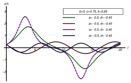
Figure 10. Performance of the OAFM-solution ${\overline{u}}_{OAFM}\left(t\right)$ of Equation (61) (dotted black curve), compared with the corresponding numerical solutions (solid color curve), respectively.

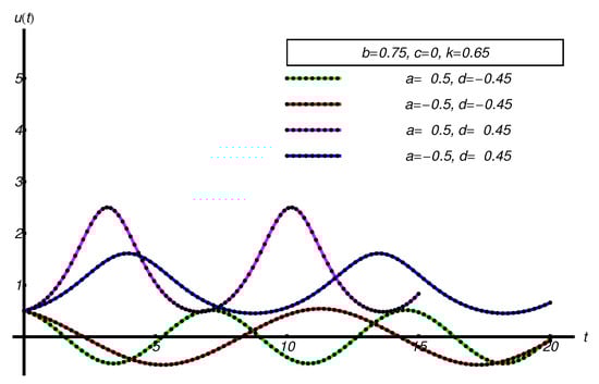
Figure 11. Performance of the OAFM-solution ${\overline{u}}_{OAFM}\left(t\right)$ of Equation (63) (dotted black curve), compared with the corresponding numerical ones (solid color curve), respectively.

Figure 12. States of the system $({\overline{x}}_{OAFM},{\overline{y}}_{OAFM},{\overline{z}}_{OAFM})$ using Equations (101)–(A3) for $x_0=0.25$, $y_0=0.5$, $z_0=1.5$; physical constants: $a=-0.5<0$, $b=0.85>0$, $c=0.75>0$, $d=-0.45<0$, $k=0.65$ compared with numerical integration: OAFM solutions (dashing black curve) and numerical results (solid color curve: green line for $x\left(t\right)$, red curve for $y\left(t\right)$, blue curve for $z\left(t\right)$), respectively.

Figure 13. Performance of the OAFM-solution ${\overline{u}}_{OAFM}\left(t\right)$ of Equation (65) (for $(a>0,d>0)$, $(a<0,d>0)$, $(a<0,d<0)$) and (67) (for $(a>0,d<0)$), respectively, (dotted black curve), compared with the corresponding numerical ones (solid color curve), respectively.

Figure 14. States of the system $({\overline{x}}_{OAFM},{\overline{y}}_{OAFM},{\overline{z}}_{OAFM})$ using Equations (101) and (A4) for $x_0=0.25$, $y_0=0.5$, $z_0=1.5$; physical constants: $a=-0.5<0$, $b=-0.85<0$, $c=0.75>0$, $d=-0.45<0$, $k=0.65$ compared with numerical integration: OAFM solutions (dashing black curve) and numerical results (solid color curve: green line for $x\left(t\right)$, red curve for $y\left(t\right)$, blue curve for $z\left(t\right)$), respectively.

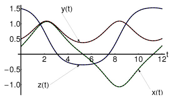
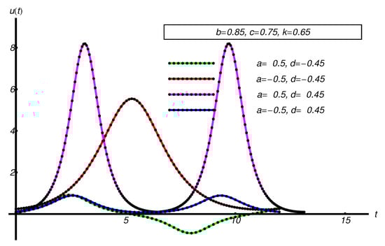
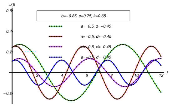
Figure 15. Performance of the OAFM-solution ${\overline{u}}_{OAFM}\left(t\right)$ of Equation (65) (dotted black curve), compared with the corresponding numerical ones (solid color curve), respectively.

Figure 16. States of the system $({\overline{x}}_{OAFM},{\overline{y}}_{OAFM},{\overline{z}}_{OAFM})$ using Equations (101) and (A5) for $x_0=0.25$, $y_0=0.5$, $z_0=1.5$; physical constants: $a=0.5>0$, $b=0.85>0$, $c=-0.75<0$, $d=-0.45<0$, $k=0.65$ compared with numerical integration: OAFM solutions (dashing black curve) and numerical results (solid color curve: green line for $x\left(t\right)$, red curve for $y\left(t\right)$, blue curve for $z\left(t\right)$), respectively.

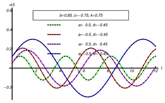
Figure 17. Performance of the OAFM-solution ${\overline{u}}_{OAFM}\left(t\right)$ of Equation (67) (dotted black curve), compared with the corresponding numerical ones (solid color curve), respectively.

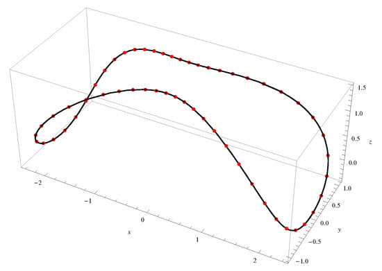
Figure 18. Periodic orbit $\left(x\left(t\right),y\left(t\right),z\left(t\right)\right)$ of Equation (67) for $a=0.5$, $b=0.85$, $c=0.75$, $d=-0.45$, $k=0.65$: OAFM-solution (dotted color curve), compared with the corresponding numerical ones (solid black curve), respectively.

Unlike the homotopy perturbation methods (requiring a large number of iterations), a first advantage of the OAFM technique is the convergence control with the index $N_{max}$.

The convergence control is regarded as a qualitative property of the OAFM-solutions as close as possible to the exact solution implicitly defined by Equations (3) and (41).

Testing is done using a rigorous numerical method such as the fourth-order Runge–Kutta method. The absolute values denoted by ${ϵ}_u=|u_{numerical}-{\overline{u}}_{OAFM}|$ are presented in the following tables.

There are 3D dynamical systems that admit only a prime integral, so the exact solution is not known, but with the help of the prime integral and the OAFM method, one can construct semi-analytic solutions in closed form.

In the case of complex dynamical systems, even with several degrees of freedom, the convergence control is more difficult and new numerical/analytical methods are sought.

Comparison with the Iterative Method

In 2006, Daftardar-Gejji et al. [26] developed an iterative method for solving nonlinear functional equations. This method is validated for a class of nonlinear functional equations (such as the Voltera-type integral equation, the nonlinear 3D- differential system, and the fractional-order differential equation) whose exact solutions are known in analytical form.

The advantage of the OAFM method compared with the iterative method described in [27] (using eight iterations) is highlighted in this subsection. In Table 21 and Figure 19, respectively, the precision and efficiency of the OAFM method can be seen.

Table 21. Values of the OAFM-solution ${\overline{x}}_{OAFM}\left(t\right)$ (A1), the iterative solution $x_{iter}\left(t\right)$, and the numerical integration.

t	${\mathit{x}}_{\mathit{numerical}}$	${\overline{\mathit{x}}}_{\mathit{OAFM}}$	${\mathit{x}}_{\mathit{iter}}$
0	0.25	0.2500000099	0.25
1/2	0.3871461205	0.3871462684	0.3871461097
1	0.5547748969	0.5547749864	0.5547748652
3/2	0.7604269013	0.7604266715	0.7604267852
2	1.0050873071	1.0050873871	1.0050857278
5/2	1.2742254393	1.2742254977	1.2742081489
3	1.5271576554	1.5271575136	1.5272332007
7/2	1.6978024263	1.6978026989	1.7009599136
4	1.7246494125	1.7246491591	1.7536803864
9/2	1.5967155859	1.5967157642	1.7306827097
5	1.3631319493	1.3631316176	1.7128681253

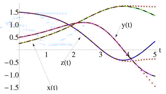
Figure 19. Performance of the approximate solutions ${\overline{x}}_{OAFM}\left(t\right)$, ${\overline{y}}_{OAFM}\left(t\right)$, ${\overline{z}}_{OAFM}\left(t\right)$ of Equation (1) using Equation (A1) (dashing black curves), compared with the iterative solutions $x_{iter}\left(t\right)$, $y_{iter}\left(t\right)$, $z_{iter}\left(t\right)$ using Equation (104) (dotted red curves) and the corresponding numerical ones (solid color curves: green for $x\left(t\right)$, magenta for $y\left(t\right)$, blue for $z\left(t\right)$), respectively.

System (1) is integrated over the interval $[0,t]$, and it obtains the following:

$$\begin{array}{c}{\displaystyle x\left(t\right)=x\left(0\right)+\underset{0}{\overset{t}{\int }}\left(ay\left(s\right)+by\left(s\right)z\left(s\right)\right)ds}\hfill \\ {\displaystyle y\left(t\right)=y\left(0\right)+\underset{0}{\overset{t}{\int }}\left(cx\left(s\right)z\left(s\right)+dx\left(s\right)\right)ds}\hfill \\ {\displaystyle z\left(t\right)=z\left(0\right)+\underset{0}{\overset{t}{\int }}\left(-kx\left(s\right)y\left(s\right)\right)ds}\hfill \end{array}.$$

(102)

The iterative algorithm leads to the following:

$$\begin{array}{c}{\displaystyle x_0\left(t\right)=x\left(0\right),x_1\left(t\right)=N_1(x_0,y_0,z_0)=\underset{0}{\overset{t}{\int }}\left(ay\left(0\right)+by\left(0\right)z\left(0\right)\right)ds,}\hfill \\ {\displaystyle y_0\left(t\right)=y\left(0\right),y_1\left(t\right)=N_2(x_0,y_0,z_0)=\underset{0}{\overset{t}{\int }}\left(cx\left(0\right)z\left(0\right)+dx\left(0\right)\right)ds,}\hfill \\ {\displaystyle z_0\left(t\right)=z\left(0\right),z_1\left(t\right)=N_3(x_0,y_0,z_0)=\underset{0}{\overset{t}{\int }}\left(-kx\left(0\right)y\left(0\right)\right)ds,}\hfill \\ \cdots \hfill \\ x_m\left(t\right)=N_1\left({\displaystyle \sum _{i=0}^{m-1}{x}_i,\sum _{i=0}^{m-1}{y}_i,\sum _{i=0}^{m-1}{z}_i}\right)-N_1\left({\displaystyle \sum _{i=0}^{m-2}{x}_i,\sum _{i=0}^{m-2}{y}_i,\sum _{i=0}^{m-2}{z}_i}\right),\hfill \\ y_m\left(t\right)=N_2\left({\displaystyle \sum _{i=0}^{m-1}{x}_i,\sum _{i=0}^{m-1}{y}_i,\sum _{i=0}^{m-1}{z}_i}\right)-N_2\left({\displaystyle \sum _{i=0}^{m-2}{x}_i,\sum _{i=0}^{m-2}{y}_i,\sum _{i=0}^{m-2}{z}_i}\right),\hfill \\ z_m\left(t\right)=N_3\left({\displaystyle \sum _{i=0}^{m-1}{x}_i,\sum _{i=0}^{m-1}{y}_i,\sum _{i=0}^{m-1}{z}_i}\right)-N_3\left({\displaystyle \sum _{i=0}^{m-2}{x}_i,\sum _{i=0}^{m-2}{y}_i,\sum _{i=0}^{m-2}{z}_i}\right),\hfill \\ m\ge 2.\hfill \end{array}$$

(103)

The iterative algorithm leads to the solution of the Equation (1) as follows:

$${\displaystyle x_{iter}\left(t\right)=\sum _{m=0}^{\infty }{x}_m\left(t\right),y_{iter}\left(t\right)=\sum _{m=0}^{\infty }{y}_m\left(t\right),z_{iter}\left(t\right)=\sum _{m=0}^{\infty }{z}_m\left(t\right),}$$

For the following initial conditions: $x\left(0\right)=0.25$, $y\left(0\right)=0.5$, $z\left(0\right)=1.5$ and physical constants $a=0.5>0$, $b=0$, $c=0.75$, $d=-0.45<0$, $k=0.65$ (presented in Table 21), the iterative solutions $x_{iter}\left(t\right)$, after eight iterations using the algorithm (103), have the following form:

$$\begin{array}{c}{\displaystyle x_{iter}\left(t\right)=\sum _{m=0}^8{x}_m\left(t\right)=0.25+0.25t+0.0421875t^2+0.0127929687t^3}\hfill \\ +0.0001272583t^4-0.0001868476t^5-0.0001127917t^6-0.0000280089t^7\hfill \\ -4.8371\times {10}^{-6}{t}^8-5.0463\times {10}^{-7}{t}^9+6.9139\times {10}^{-8}{t}^{10}+4.3810\times {10}^{-8}{t}^{11}\hfill \\ +1.2752\times {10}^{-8}{t}^{12}+2.4153\times {10}^{-9}{t}^{13}+2.8401\times {10}^{-10}{t}^{14}-4.4590\times {10}^{-12}{t}^{15}\hfill \\ -1.2718\times {10}^{-11}{t}^{16}-3.8729\times {10}^{-12}{t}^{17}+\mathcal{O}\left({10}^{-13}\right);\hfill \\ {\displaystyle y_{iter}\left(t\right)=\sum _{m=0}^8{y}_m\left(t\right)=0.5+0.16875t+0.0767578125t^2}\hfill \\ +0.0010180664t^3-0.0018684768t^4-0.0013535010t^5-0.0003921249t^6\hfill \\ -0.0000773944t^7-8.9987\times {10}^{-6}{t}^8+1.3144\times {10}^{-6}{t}^9\hfill \\ +9.5956\times {10}^{-7}{t}^{10}+3.1557\times {10}^{-7}{t}^{11}+6.7129\times {10}^{-8}{t}^{12}+8.9845\times {10}^{-9}{t}^{13}\hfill \\ -1.4733\times {10}^{-10}{t}^{14}-5.1401\times {10}^{-10}{t}^{15}-1.8139\times {10}^{-10}{t}^{16}-4.1114\times {10}^{-11}{t}^{17}\hfill \\ -6.1228\times {10}^{-12}{t}^{18}+\mathcal{O}\left({10}^{-13}\right);\hfill \\ {\displaystyle z_{iter}\left(t\right)=\sum _{m=0}^8{z}_m\left(t\right)=1.5-0.081250t-0.0543359375t^2}\hfill \\ -0.0178686523t^3-0.0053559341t^4-0.0006822478t^5-0.0000159755t^6\hfill \\ +0.0000538912t^7+0.0000199578t^8+5.1792\times {10}^{-6}{t}^9\hfill \\ +8.6714\times {10}^{-7}{t}^{10}+4.8166\times {10}^{-8}{t}^{11}-2.8151\times {10}^{-8}{t}^{12}-1.3599\times {10}^{-8}{t}^{13}\hfill \\ -3.6087\times {10}^{-9}{t}^{14}-6.5933\times {10}^{-10}{t}^{15}-6.1959\times {10}^{-11}{t}^{16}+9.3548\times {10}^{-12}{t}^{17}\hfill \\ +6.2900\times {10}^{-12}{t}^{18}+1.7947\times {10}^{-12}{t}^{19}+\mathcal{O}\left({10}^{-13}\right).\hfill \end{array}$$

(104)

Figure 19 shows the the OAFM solutions ${\overline{x}}_{OAFM}$, ${\overline{y}}_{OAFM}$, ${\overline{z}}_{OAFM}$, compared with the corresponding iterative solutions given in Equation (104) and the corresponding numerical ones. This comparison reflects the accuracy of the OAFM approach using only one iteration.

6. Conclusions

The present paper is dedicated to developing the OAFM analytical approach for a class of dynamical system. This dynamical system admits two prime integrals (constants of motion), involving the existence of symmetry with respect to the $Oz$-axis and the existence of periodic, homoclinic, or heteroclinic orbits. Good agreement between the OAFM results and the corresponding numerical ones is demonstrated in this work. The comparative analysis reflects the accuracy of the method, as the obtained solutions are close to the exact solution. The advantages of the OAFM method compared with the iterative method are synthesized by the following:

• The arbitrary choice of the linear operator L and auxiliary functions $A_j$ allows us to write the OAFM-solution in an effective form;
• The convergence control (in the sense that the residual functions are smaller than 1): The auxiliary functions depend on the finite number of the unknown parameters which could be optimally computed to obtain the absolute values between the semi-analytical solutions and numerical ones smaller than 1;
• The non-existence of small parameters: The OAFM-solutions are built for arbitrary values for the physical parameters a, b, c, d, k, namely, for $ac-bd\ne 0$ in all subcases $bc=0$, $bc>0$, and $bc<0$, respectively; A special case when $ac-bd=0$ is analytically investigated. The OAFM-solution is obtained in the same manner.
• The efficiency is highlighted by the comparison between the OAFM-solutions with the corresponding iterative solutions, more specifically, the iterative method is validated only when the exact solution is known; on the other hand, by the OAFM method, the exact solution is approximated by arbitrarily choosing the auxiliary functions and optimally finding the unknown parameters, proving the accuracy of the OAFM-results.

The achievement of these results encourages the study of dynamical systems with similar properties as models that can describe physical and biological problems as follows: the change in the energy levels of an atom with two levels as a function of the eigenvalue; or in biology, the bi-Hamiltonian structure of Kermack and McKendrick modeling for the spread of epidemics in a closed population.

References

- Xu, M.; Shi, S.; Huang, K. The connection between the dynamical properties of 3D systems and the image of the energy-Casimir mapping. Discrete Contin. Dyn. Syst. AIMS 2024, 44, 791–807. [Google Scholar] [CrossRef]
- Lazureanu, C. On the Hamilton–Poisson realizations of the integrable deformations of the Maxwell-Bloch equations. C. R. Math. 2017, 355, 596–600. [Google Scholar] [CrossRef]
- Lazureanu, C. Hamilton–Poisson Realizations of the Integrable Deformations of the Rikitake System. Adv. Math. Phys. 2017, 2017, 4596951. [Google Scholar]
- Tudoran, R.M.; Girban, A. On the completely integrable case of the Rössler system. J. Math. Phys. 2012, 53, 052701. [Google Scholar] [CrossRef]
- Gümral, H.; Nutku, Y. Poisson structure of dynamical systems with three degrees of freedom. J. Math. Phys. 1993, 34, 5691. [Google Scholar] [CrossRef]
- Lazureanu, C.; Cho, J. On a family of Hamilton–Poisson Jerk System. Mathematics 2024, 12, 1260. [Google Scholar] [CrossRef]
- Tudoran, R.M.; Aron, A.; Nicoara, S. On a Hamiltonian version of the Rikitake system. SIAM J. Appl. Dyn. Syst. 2009, 8, 454–479. [Google Scholar] [CrossRef]
- Tudoran, R.M.; Tudoran, R.A. On a large class of three-dimensional Hamiltonian systems. J. Math. Phys. 2009, 50, 012703. [Google Scholar] [CrossRef]
- Lazuranu, C.; Binzar, T. Symmtries of some classes of dynamical systems. J. Nonlinear Math. Phy. 2015, 22, 265–274. [Google Scholar]
- Lazureanu, C.; Hedrea, C.; Petrisor, C. On a deformed version of the two-disk dynamo system. Appl. Math. 2021, 66, 345–372. [Google Scholar] [CrossRef]
- Giné, J.; Sinelshchikov, D.I. On the geometric and analytical properties of the anharmonic oscillator. Commun. Nonlinear Sci. 2024, 131, 107875. [Google Scholar] [CrossRef]
- Marinca, V.; Herisanu, N. Approximate analytical solutions to Jerk equation. In Springer Proceedings in Mathematics & Statistics: Proceedings of the Dynamical Systems: Theoretical and Experimental Analysis, Lodz, Poland, 7–10 December 2015; Springer: Cham, Switzerland, 2016; Volume 182, pp. 169–176. [Google Scholar]
- Lazureanu, C.; Binzar, T. On the symmetries of a Rikitake type system. C. R. Math. Acad. Sci. Paris 2012, 350, 529–533. [Google Scholar]
- Xu, M.; Shi, S.; Huang, K. On the integrable stretch-twist-fold flow: Bi-Hamiltonian structures and global dynamics. J. Math. Phys. 2024, 65, 022704. [Google Scholar] [CrossRef]
- Huang, K.; Shi, S.; Xu, Z. Integrable deformations, bi-Hamiltonian structures and nonintegrability of a generalized Rikitake system. Int. J. Geom. Methods Mod. Phys. 2019, 16, 1950059. [Google Scholar] [CrossRef]
- Biggs, R.; Remsing, C.C. Quadratic Hamilton–Poisson Systems in Three Dimensions: Equivalence, Stability, and Integration. Acta Appl. Math. 2017, 148, 1–59. [Google Scholar] [CrossRef]
- Olver, P.J. Applications of Lie Groups to Differential Equations; Springer: New York, NY, USA, 1986. [Google Scholar]
- Krishnaprasad, P.S. Lie–Poisson structures, dual-spin spacecraft and asymptotic stability. Nonlinear Anal. Theory Methods Appl. 1985, 9, 1011–1035. [Google Scholar]
- David, D.; Holm, D.D. Multiple Lie–Poisson Structures, Reductions, and Geometric Phases for the Maxwell-Bloch Travelling Wave Equations. J. Nonlinear Sci. 1992, 2, 241–262. [Google Scholar]
- Rikitake, T. Oscillations of a system of disk dynamos. Proc. Camb. Philos. Soc. 1958, 54, 89–105. [Google Scholar] [CrossRef]
- Pikovskii, A.S.; Rabinovich, M.I. Stochastic behavior of dissipative systems. Soc. Sci. Rev. C Math. Phys. Rev. 1981, 2, 165–208. [Google Scholar]
- Chen, H.-K.; Lee, C.-I. Anti-control of chaos in rigid body motion. Chaos Soliton Fract. 2004, 21, 957–965. [Google Scholar] [CrossRef]
- Ene, R.-D.; Pop, N. Semi-Analytical Solutions for the Qi–Type Dynamical System. Symmetry 2024, 16, 1578. [Google Scholar] [CrossRef]
- Marinca, V.; Ene, R.-D.; Marinca, V.B. Optimal Auxiliary Functions Method for viscous flow due to a stretching surface with partial slip. Open Eng. 2018, 8, 261–274. [Google Scholar]
- Ene, R.-D.; Pop, N.; Lapadat, M. Approximate Closed-Form Solutions for the Rabinovich System via the Optimal Auxiliary Functions Method. Symmetry 2022, 14, 2185. [Google Scholar] [CrossRef]
- Ene, R.-D.; Pop, N.; Lapadat, M.; Dungan, L. Approximate closed-form solutions for the Maxwell-Bloch equations via the Optimal Homotopy Asymptotic Method. Mathematics 2022, 10, 4118. [Google Scholar] [CrossRef]
- Daftardar-Gejji, V.; Jafari, H. An iterative method for solving nonlinear functional equations. J. Math. Anal. Appl. 2006, 316, 753–763. [Google Scholar]
Disclaimer/Publisher’s Note: The statements, opinions and data contained in all publications are solely those of the individual author(s) and contributor(s) and not of MDPI and/or the editor(s). MDPI and/or the editor(s) disclaim responsibility for any injury to people or property resulting from any ideas, methods, instructions or products referred to in the content. |
© 2025 by the authors. Licensee MDPI, Basel, Switzerland. This article is an open access article distributed under the terms and conditions of the Creative Commons Attribution (CC BY) license (https://creativecommons.org/licenses/by/4.0/).