Orbit Determination of Impulsively Maneuvering Spacecraft Using Adaptive State Noise Compensation

Abstract

Accurate orbit determination (OD) for spacecraft with impulsive maneuvers in a multi-body system is a challenging task, because the unknown magnitudes and epochs of the maneuvers make dynamic modeling difficult, disrupting the symmetry of state deviations before and after the maneuvers. This paper proposes an Adaptive State Noise Compensation (ASNC) algorithm for the OD of spacecraft with impulsive maneuvering in a three-body dynamics frame, which does not rely on maneuver parameters and can adaptively estimate state noise. Firstly, a decoupled matching factor is developed, which can be used to identify the maneuvering and non-maneuvering epochs of the target spacecraft. Next, based on the matching factor, a position state noise estimation method is presented. Moreover, a method for estimating velocity state noise through inverse mapping of the state transition matrix is formulated, and the compensated state noise is incorporated into the Kalman framework to achieve precise OD of maneuvering spacecraft. Finally, the proposed method is applied to solve the OD problem of a Near Rectilinear Halo Orbit (NRHO) near the Earth–Moon L2 point. Simulation results demonstrated that the proposed method improved accuracy by at least an order of magnitude compared to competitive methods, while effectively restoring the symmetry of the OD system.

1. Introduction

Orbit determination (OD) is a critical task in space missions, as accurate knowledge of a spacecraft’s state is the foundation for subsequent operations such as guidance and control [1,2,3]. Existing methods have been effective in solving the problem for non-maneuvering spacecraft. However, most spacecraft in space need to perform maneuvers to address various mission tasks, such as orbit maintenance [4,5], rendezvous and docking, and space object detection [6,7,8,9]. Due to the lack of prior information about the magnitude and epoch of unknown maneuvers for non-cooperative spacecraft, accurately modeling a spacecraft’s dynamics becomes challenging [10,11], disrupting the symmetry of state deviations before and after the maneuvers. Without compensating for the unmodeled dynamics, the accuracy of OD will degrade or even diverge [12].

Maneuvering spacecraft OD techniques can be classified into three main categories: OD reinitiating, maneuver reconstruction, and filter-based methods. OD reinitiating methods involve restarting the OD process once a maneuver has been detected [13,14]. However, OD reinitiating methods disregard the pre-maneuver solutions and measurements, focusing only on determining a new orbit after the maneuver has been detected [9].

Maneuver reconstruction techniques estimate both the state and maneuver of the target spacecraft by using measurements before and after the maneuver. Lubey et al. [15] proposed an optimal control-based estimator (OCBE) for maneuver reconstruction in geostationary orbits (GEO), improving OD accuracy. Serra et al. [16] developed a method to associate optical observations with orbits under unknown maneuvers, improving OD accuracy through simultaneous state and maneuver estimation. Tang et al. [17] addressed the impact of shadow effects on OD in Earth–Moon Lagrange point L2 orbits, incorporating orbital changes before and after maneuvers. Wang et al. [18] improved OD accuracy with a kinematic model, while Zhou et al. [19] introduced a state transition tensor (STT)-based method for precise maneuver reconstruction. Although these techniques can enhance OD accuracy, they involve high computational complexity and are impractical for real-time applications.

Filter-based methods improve the filter structure, to handle unknown maneuvers and compensate for the lack of prior information. Unlike maneuver reconstruction, they integrate post-maneuver data into the pre-maneuver orbit in real time, enabling sequential OD and real-time spacecraft tracking. Chul et al. [20] proposed an Extended Kalman Filter (EKF) method using Thrust-Fourier-Coefficients (TFC) for real-time tracking of maneuvering satellites, handling OD without prior assumptions about the maneuver. Jiang et al. [21] developed a residual-normalized Strong Tracking Filter (STF), improving the sensitivity to small impulsive maneuvers, especially for uncooperative spacecraft. Guang et al. [22] introduced a Variable Structure Estimator (VSE) for continuous maneuvers, achieving stable orbit estimates by adaptively adjusting the Kalman filter covariance. Zhou et al. [23] proposed the Polynomial Approximation Method (PAM) within an EKF framework for spacecraft OD with unknown maneuvers, achieving high accuracy in various scenarios. While effective for continuous thrust, PAM’s performance diminishes with long observation intervals or large impulsive maneuvers.

The multiple-model adaptive estimator for OD uses a set of Kalman filters, each corresponding to a specific maneuvering dynamic. Proposed by Maybeck and Hentz, this approach adapts to different maneuver models for maneuvering targets [24]. Lee et al. [25] proposed a state-dependent adaptive estimation method for impulsively maneuvering spacecraft, using two models—maneuvering and non-maneuvering—and state-dependent transition probabilities to effectively handle orbit discontinuities. The algorithm provides good OD accuracy for impulsively maneuvering spacecraft, but its applicability is limited by requiring prior information of the target spacecraft’s maneuvers. Additionally, deep learning techniques have been applied to maneuvering target OD [26], including maneuver detection [27], classification [28], and orbit prediction [29,30].

Compared with maneuver reconstruction methods, filter-based methods have much lower computational burdens [31,32]. Moreover, filter-based methods can effectively leverage pre-maneuver measurements and dynamic information, offering higher accuracy than OD reinitiating methods. However, current filter-based OD methods still have certain limitations. Current variable-structure filtering methods are more suitable for continuous thrust maneuvers, and their OD performance degrades or even diverges when faced with long observation intervals or large-magnitude impulsive maneuvers of the target spacecraft. Additionally, OD methods for impulsively maneuvering spacecraft often rely on prior information about the magnitude and epoch of the spacecraft’s maneuvers, making them unsuitable for uncooperative spacecraft.

This paper proposes an Adaptive State Noise Compensation (ASNC) method for the OD of impulsively maneuvering spacecraft, where prior maneuver information is unknown. It models the state deviations caused by unknown impulsive maneuvers as state noise and, within the framework of Kalman filtering, can adaptively compensate for the inaccuracies in dynamic modeling caused by unknown maneuvers. First, the proposed Noise Matching Factor (NMF) uses standardized and squared innovations to detect impulsive maneuvers by comparing the NMF with a historical mean indicator. When the difference exceeds a threshold, a maneuver is detected. The state noise is modeled as a piecewise function, set to zero when no maneuver is detected, ensuring efficient algorithm performance. Next, an adaptive method for estimating state noise is proposed. For position state noise, a matching-based estimation aligns the current NMF with the indicator function. A linear system of equations is derived, and the least squares method is used for over-determined cases, while zero-value compensation ensures coverage of position deviations in under-determined cases, ensuring OD algorithm convergence. Meanwhile, for velocity state noise, an estimation method via inverse is proposed, which uses a state transition matrix to establish the mapping between position and velocity deviations after the impulsive maneuver. Finally, the adaptively compensated state noise is incorporated into the framework of Kalman filtering to compensate for the inaccurately modeled dynamics, thereby achieving precise OD for spacecraft with impulsive maneuvers.

The remainder of this paper is organized as follows: Section 2 introduces the state model and measurement model, followed by the algorithm framework. Section 3 presents the spacecraft maneuver detection indicators and the ASNC strategy. Section 4 covers the simulation results, and Section 5 concludes the paper.

2. System Model & Preliminary

2.1. System Model

The differential equation of the state vector for the spacecraft is

$${\dot{\mathit{x}}}_k=\mathit{f}\left({\mathit{x}}_k\right)=\left[\begin{array}{c}{\dot{\mathit{r}}}_k\\ {\dot{\mathit{v}}}_k\end{array}\right]={\left[{\dot{x}}_k{\dot{y}}_k{\dot{z}}_k{\ddot{x}}_k{\ddot{y}}_k{\ddot{z}}_k\right]}^T.$$

(1)

where ${\mathit{x}}_k\in {\mathbb{R}}^6$ is the state vector of the spacecraft; ${\mathit{r}}_k={\left[x_k{y}_k{z}_k\right]}^T\in {\mathbb{R}}^3$ is the position vector of the spacecraft at epoch k; ${\mathit{v}}_k={\left[{\dot{x}}_k{\dot{y}}_k{\dot{z}}_k\right]}^T\in {\mathbb{R}}^3$ is the velocity vector of the spacecraft at epoch k.

The state model for impulsively maneuvering can be expressed as

$${\dot{\mathit{x}}}_k=\mathit{F}\left({\mathit{x}}_{k-1}\right)+{\delta }_{t,k}\mathrm{\Delta }{\mathit{x}}_k.$$

(2)

Here, ${\delta }_{t,k}$ represents the Kronecker delta, where ${\delta }_{t,k}=0$ when $t\ne k$, and ${\delta }_{t,k}=1$ when $t=k$; $\mathrm{\Delta }{\mathit{x}}_k=\left[\mathrm{\Delta }{\mathit{x}}_k^r\mathrm{\Delta }{\mathit{x}}_k^v\right]={\left[\mathrm{\Delta }{x}_{k,1}\mathrm{\Delta }{x}_{k,2}\mathrm{\Delta }{x}_{k,3}\mathrm{\Delta }{x}_{k,4}\mathrm{\Delta }{x}_{k,5}\mathrm{\Delta }{x}_{k,6}\right]}^T\in {\mathbb{R}}^6$ represents the state deviation resulting from impulsively maneuvering and is considered as state noise in the OD algorithm; and $\mathit{F}\left({\mathit{x}}_{k-1}\right)$ indicates the state propagation based on the differential Equation (1) for the state vector of the spacecraft.

The differential equation for the State Transition Matrix (STM) of the state model described in Equation (2) is

$${\dot{\mathbf{\Phi }}}_k=\mathit{A}\left({\mathit{x}}_{k\mathit{-}1}\right){\mathbf{\Phi }}_k.$$

(3)

where

$$\mathit{A}\left({\mathit{x}}_{k-1}\right)={\displaystyle \frac{\partial \mathit{f}}{\partial \mathit{x}}}{|}_{\mathit{x}={\mathit{x}}_{k-1}}$$

(4)

is the Jacobian matrix of the state model.

The measurement model is expressed as

$${\mathit{z}}_k=\left[\begin{array}{c}{z}_{k,1}\\ ⋮\\ z_{k,p}\end{array}\right]=\mathit{h}\left({\mathit{x}}_k\right)+{\mathit{\nu }}_k=\left[\begin{array}{c}{h}_1\left({\mathit{x}}_k\right)\\ ⋮\\ h_p\left({\mathit{x}}_k\right)\end{array}\right]+{\mathit{\nu }}_k,$$

(5)

$$E\left({\mathit{\nu }}_k{\mathit{\nu }}_k^T\right)={\mathit{R}}_k=\left[\begin{array}{ccccc}{R}_{11}& 0& \cdots & 0& 0\\ 0& ⋮& 0& 0& 0\\ ⋮& 0& R_{ii}& 0& \cdots \\ 0& 0& 0& ⋮& 0\\ 0& 0& 0& \cdots & R_{pp}\end{array}\right].$$

(6)

where ${\mathit{z}}_k\in {\mathbb{R}}^p$ represents the p-dimensional measurement vector; $\mathit{h}:{\mathbb{R}}^6\to {\mathbb{R}}^p$ represents the mapping from the state to the measurement; and ${\mathit{\nu }}_k\in {\mathbb{R}}^p$ represents Gaussian white noise with zero mean, and its covariance matrix is ${\mathit{R}}_k$.

2.2. EKF Algorithm

2.2.1. Prediction Step

The predicted states are given as

$${\widehat{\mathit{x}}}_k^{-}=\mathit{F}\left({\widehat{\mathit{x}}}_{k-1}\right).$$

(7)

where ${\widehat{\mathit{x}}}_k^{-}\in {\mathbb{R}}^6$ is the predicted state at epoch $k+1$; ${\widehat{\mathit{x}}}_{k-1}\in {\mathbb{R}}^6$ is the estimated state at epoch $k-1$; and $\mathit{F}(·)$ is the state propagation model described in Equation (2).

The predicted covariance matrix is given as

$${\mathit{P}}_k^{-}={\mathbf{\Phi }}_k{\mathit{P}}_{k-1}{\mathbf{\Phi }}_k^T+{\mathit{Q}}_k.$$

(8)

2.2.2. Update Step

Upon receiving the measurement ${\mathit{z}}_k$, the estimated state ${\widehat{\mathit{x}}}_k$ and the covariance matrix ${\mathit{P}}_{k+1}$ are updated using the following equations:

$${\mathit{K}}_k={\mathit{P}}_k^{-}{\mathit{H}}_k^T{\left[{\mathit{H}}_k{\mathit{P}}_k^{-}{\mathit{H}}_k^T+{\mathit{R}}_k\right]}^{-1},$$

(9)

$${\widehat{\mathit{x}}}_k={\widehat{\mathit{x}}}_k^{-}+{\mathit{K}}_k\left({\mathit{z}}_k-\mathit{h}\left({\widehat{\mathit{x}}}_k^{-}\right)\right),$$

(10)

$${\mathit{P}}_k={(\mathit{I}-{\mathit{K}}_k)}^T{\mathit{P}}_k^{-}(\mathit{I}-{\mathit{K}}_k{\mathit{H}}_k)+{\mathit{K}}_k^T{\mathit{R}}_k{\mathit{K}}_k.$$

(11)

where ${\mathit{R}}_k$ is the covariance matrix of the measurement noise,

$${\mathit{H}}_k=\left[\begin{array}{c}{\mathit{H}}_{k,1}\\ ⋮\\ {\mathit{H}}_{k,i}\\ ⋮\\ {\mathit{H}}_{k,p}\end{array}\right]={\displaystyle \frac{\partial \mathit{h}}{\partial \mathit{x}}}{|}_{\mathit{x}={\widehat{\mathit{x}}}_k^{-}}=\left[\begin{array}{c}{\displaystyle \frac{\partial h_1}{\partial \mathit{x}}}{|}_{\mathit{x}={\widehat{\mathit{x}}}_k^{-}}\\ ⋮\\ {\displaystyle \frac{\partial h_i}{\partial \mathit{x}}}{|}_{\mathit{x}={\widehat{\mathit{x}}}_k^{-}}\\ ⋮\\ {\displaystyle \frac{\partial h_p}{\partial \mathit{x}}}{|}_{\mathit{x}={\widehat{\mathit{x}}}_k^{-}}\end{array}\right]$$

(12)

is the Jacobian matrix of the measurement model.

3. ASNC Method

3.1. Noise Matching Factor (NMF)

Innovation is a common metric for assessing the consistency of the filter, and it can be used to calculate the match between the actual measurements and the filter’s estimated state. The innovation ${\mathit{\gamma }}_k$ is given as

$${\mathit{\gamma }}_k=\left[\begin{array}{c}{\gamma }_{k,1}\\ ⋮\\ {\gamma }_{k,i}\\ ⋮\\ {\gamma }_{k,p}\end{array}\right]={\mathit{z}}_k-\mathit{h}\left({\widehat{\mathit{x}}}_k^{-}\right)=\left[\begin{array}{c}{z}_{k,1}-h_1\left({\widehat{\mathit{x}}}_k^{-}\right)\\ ⋮\\ z_{k,i}-h_i\left({\widehat{\mathit{x}}}_k^{-}\right)\\ ⋮\\ z_{k,p}-h_p\left({\widehat{\mathit{x}}}_k^{-}\right)\end{array}\right].$$

(13)

where the variance $S_{k,i}$ in ${\gamma }_{k,i}$ is

$$S_{k,i}={\mathit{H}}_{k,i}{\mathit{P}}_k^{-}{\mathit{H}}_{k,i}^T+R_{ii}.$$

(14)

The standardized square result ${\mathrm{\Lambda }}_{k,i}$ of ${\gamma }_{k,i}$ is

$${\mathrm{\Lambda }}_{k,i}={\gamma }_{k,i}^2/S_{k,i}.$$

(15)

Under the linearization assumption, each dimension of ${\gamma }_k\in {\mathbb{R}}^p$ follows a Gaussian distribution. Each dimension of ${\gamma }_k$ is standardized and squared to construct the NMF

$${\mathbf{\Lambda }}_k=\left[\begin{array}{c}{\mathrm{\Lambda }}_{k,1}\\ ⋮\\ {\mathrm{\Lambda }}_{k,i}\\ ⋮\\ {\mathrm{\Lambda }}_{k,p}\end{array}\right]=\left[\begin{array}{c}{\gamma }_{k,1}^2/S_{k,1}\\ ⋮\\ {\gamma }_{k,i}^2/S_{k,i}\\ ⋮\\ {\gamma }_{k,p}^2/S_{k,p}\end{array}\right]=\left[\begin{array}{c}{\gamma }_{k,1}^2/\left({\mathit{H}}_{k,1}{\mathit{P}}_k^{-}{\mathit{H}}_{k,1}^T+R_{11}\right)\\ ⋮\\ {\gamma }_{k,i}^2/\left({\mathit{H}}_{k,i}{\mathit{P}}_k^{-}{\mathit{H}}_{k,i}^T+R_{ii}\right)\\ ⋮\\ {\gamma }_{k,p}^2/\left({\mathit{H}}_{k,p}{\mathit{P}}_k^{-}{\mathit{H}}_{k,p}^T+R_{pp}\right)\end{array}\right].$$

(16)

where ${\mathbf{\Lambda }}_k$ is a p-dimensional vector, which results from independently analyzing the innovations corresponding to each channel of the measurement ${\mathit{z}}_k$. The rationale for this approach lies in the fact that, during the actual measurement process, considering factors such as different sensors providing information, the sampling precision of the same sensor, and uncertainties in the algorithms processing the measurement information, each dimension of ${\mathit{z}}_k$ can be approximately regarded as following an independent Gaussian distribution. The advantages of this approach are (1) it avoids the complexity of matrix inversion when coupling the measurement information to solve the covariance matrix, simplifying the analysis; and (2) ${\mathbf{\Lambda }}_k$ retains the multi-dimensional characteristics of the measurement information as a p-dimensional vector, which can more accurately reflect the OD performance.

When the spacecraft is not maneuvering, the dynamics model in the OD algorithm aligns with the actual situation. Therefore, the mean of the NMF from the initial epoch to epoch $k-1$ is used as the indicator function

$${\mathit{\mu }}_{k-1}={\displaystyle \frac{\left({\mathit{\mu }}_{k-2}\times (k-2)+{\mathbf{\Lambda }}_{k-1}\right)}{k-1}}.$$

(17)

where ${\mathit{\mu }}_0=0$ is set as the initial value.

The covariance matrix of the state noise for the state model in Equation (8) can be modeled as

$${\mathit{Q}}_k=\left\{\begin{array}{cc}{\mathit{O}}_{3\times 3}\hfill & \mathrm{if}{\displaystyle \frac{{∥{\mathit{\mu }}_{k-1}-{\mathbf{\Lambda }}_k∥}_2}{\parallel {\mathit{\mu }}_{k-1}{\parallel }_2}}\le \eta \hfill \\ \left[\begin{array}{cc}{\mathit{Q}}_k^r& {\mathit{O}}_{3\times 3}\\ {\mathit{O}}_{3\times 3}& {\mathit{Q}}_k^v\end{array}\right]\hfill & \mathrm{if}{\displaystyle \frac{{∥{\mathit{\mu }}_{k-1}-{\mathbf{\Lambda }}_k∥}_2}{\parallel {\mathit{\mu }}_{k-1}{\parallel }_2}}>\eta \hfill \end{array}\right..$$

(18)

where ${\mathit{O}}_{3\times 3}$ represents a $3\times 3$ zero matrix, ${\mathit{Q}}_k^r=\mathrm{diag}(\mathrm{\Delta }{x}_{k,1}^2,\mathrm{\Delta }{x}_{k,2}^2,\mathrm{\Delta }{x}_{k,3}^2)$ represents the position state noise covariance matrix, ${\mathit{Q}}_k^v=\mathrm{diag}(\mathrm{\Delta }{x}_{k,4}^2,\mathrm{\Delta }{x}_{k,5}^2,\mathrm{\Delta }{x}_{k,6}^2)$ represents the velocity state noise covariance matrix, and $\eta$ is the threshold value used to determine whether a sudden change has occurred in the system.

3.2. Position State Noise Estimation via Match

Regarding the OD problem of non-cooperative spacecraft, ranging and angle measurement techniques are more mature and reliable for the OD of non-cooperative spacecraft. Obtaining velocity measurement information typically requires higher equipment precision and signal processing capabilities, which is challenging to achieve in the practical operation of non-cooperative spacecraft. Therefore, this paper only considers position-related measurements and partitions the matrix ${\mathit{H}}_k$ as

$${\mathit{H}}_k=\left[\begin{array}{cc}{\mathit{H}}_k^r& {\mathit{O}}_{p\times 3}\end{array}\right].$$

(19)

where ${\mathit{H}}_k^r$ represents the Jacobian matrix obtained by taking the partial derivatives with respect to position, and ${\mathit{O}}_{p\times 3}$ represents a $p\times 3$ zero matrix.

When the condition ${∥{\mathit{\mu }}_{k-1}-{\mathbf{\Lambda }}_k∥}_2/\parallel {\mathit{\mu }}_{k-1}{\parallel }_2>\eta$ is satisfied for Equation (18), state noise compensation is applied to the covariance matrix of the predicted results, which is updated as

$${\mathit{P}}_{k,\delta }^{-}={\mathbf{\Phi }}_k{\mathit{P}}_k{\mathbf{\Phi }}_k^T+{\mathit{Q}}_k.$$

(20)

where $\delta$ is the identifier used by the NMF to detect when the target spacecraft has performed a maneuver.

The NMF at the maneuver epoch is expressed as

$${\mathbf{\Lambda }}_{k,\delta }=\left[\begin{array}{c}{\displaystyle \frac{{\gamma }_{k,1}^2}{\left({\mathit{H}}_{k,1}{\mathit{P}}_{k,\delta }^{-}{\mathit{H}}_{k,1}^T+{\mathit{H}}_{k,1}{\mathit{Q}}_k{\mathit{H}}_{k,1}^T+{\mathit{R}}_{11}\right)}}\\ ⋮\\ {\displaystyle \frac{{\gamma }_{k,i}^2}{\left({\mathit{H}}_{k,i}{\mathit{i}}_{k,\delta }^{-}{\mathit{H}}_{k,i}^T+{\mathit{H}}_{k,i}{\mathit{Q}}_k{\mathit{H}}_{k,i}^T+{\mathit{R}}_{ii}\right)}}\\ ⋮\\ {\displaystyle \frac{{\gamma }_{k,p}^2}{\left({\mathit{H}}_{k,p}{\mathit{P}}_{k,\delta }^{-}{\mathit{H}}_{k,p}^T+{\mathit{H}}_{k,p}{\mathit{Q}}_k{\mathit{H}}_{k,p}^T+{\mathit{R}}_{pp}\right)}}\end{array}\right]=\left[\begin{array}{c}{\displaystyle \frac{{\gamma }_{k,1}^2}{\left({\mathit{H}}_{k,1}{\mathit{P}}_{k,\delta }^{-}{\mathit{H}}_{k,1}^T+{\mathit{H}}_{k,1}^r{\mathit{Q}}_k^r{\mathit{H}}_{k,1}^T+{\mathit{R}}_{11}\right)}}\\ ⋮\\ {\displaystyle \frac{{\gamma }_{k,i}^2}{\left({\mathit{H}}_{k,i}{\mathit{i}}_{k,\delta }^{-}{\mathit{H}}_{k,i}^T+{\mathit{H}}_{k,i}^r{\mathit{Q}}_k^r{\mathit{H}}_{k,i}^T+{\mathit{R}}_{ii}\right)}}\\ ⋮\\ {\displaystyle \frac{{\gamma }_{k,p}^2}{\left({\mathit{H}}_{k,p}{\mathit{P}}_{k,\delta }^{-}{\mathit{H}}_{k,p}^T+{\mathit{H}}_{k,p}^r{\mathit{Q}}_k^r{\mathit{H}}_{k,p}^T+{\mathit{R}}_{pp}\right)}}\end{array}\right].$$

(21)

Since the dynamics model is accurate when no maneuver occurs, the indicator function ${\mathit{\mu }}_{k-1}$ is set equal to the NMF ${\mathbf{\Lambda }}_{k,\delta }$, forming a system of equations with respect to ${\mathit{Q}}_k^r$, as given by

$${\mathrm{\Lambda }}_{k,\delta }={\mathit{\mu }}_{k-1}.$$

(22)

Substituting Equations (21) and (17) into Equation (22), the linear system of equations for ${\mathit{Q}}_k^r$ is derived as

$$\left[\begin{array}{c}{\mathit{H}}_{k,1}^r{\mathit{Q}}_k^r{\mathit{H}}_{k,1}^T\\ ⋮\\ {\mathit{H}}_{k,i}^r{\mathit{Q}}_k^r{\mathit{H}}_{k,i}^T\\ ⋮\\ {\mathit{H}}_{k,p}^r{\mathit{Q}}_k^r{\mathit{H}}_{k,p}^T\end{array}\right]=\left[\begin{array}{c}{\displaystyle \frac{{\gamma }_{k,1}^2}{{\mu }_{k,1}-S_{k,1}}}\\ ⋮\\ {\displaystyle \frac{{\gamma }_{k,i}^2}{{\mu }_{k,i}-S_{k,i}}}\\ ⋮\\ {\displaystyle \frac{{\gamma }_{k,p}^2}{{\mu }_{k,p}-S_{k,p}}}\end{array}\right].$$

(23)

Then, by substituting Equations (18) and (23), the linear system of equations for $\mathit{X}={[\mathrm{\Delta }{x}_{k,1}^2,\mathrm{\Delta }{x}_{k,2}^2,\mathrm{\Delta }{x}_{k,3}^2]}^T$ is

$$\left[\begin{array}{ccc}{H_{k,11}^r}^2& {H_{k,12}^r}^2& {H_{k,13}^r}^2\\ ⋮& ⋮& ⋮\\ {H_{k,i1}^r}^2& {H_{k,i2}^r}^2& {H_{k,i3}^r}^2\\ ⋮& ⋮& ⋮\\ {H_{k,p1}^r}^2& {H_{k,p2}^r}^2& {H_{k,p3}^r}^2\end{array}\right]\left[\begin{array}{c}\mathrm{\Delta }{x}_{k,1}^2\\ \mathrm{\Delta }{x}_{k,2}^2\\ \mathrm{\Delta }{x}_{k,3}^2\end{array}\right]=\left[\begin{array}{c}{\displaystyle \frac{{\gamma }_{k,1}^2}{{\mu }_{k,1}-S_{k,1}}}\\ ⋮\\ {\displaystyle \frac{{\gamma }_{k,i}^2}{{\mu }_{k,i}-S_{k,i}}}\\ ⋮\\ {\displaystyle \frac{{\gamma }_{k,p}^2}{{\mu }_{k,p}-S_{k,p}}}\end{array}\right].$$

(24)

For the sake of simplicity, we define

$$\mathit{A}=\left[\begin{array}{ccc}{H_{k,11}^r}^2& {H_{k,12}^r}^2& {H_{k,13}^r}^2\\ ⋮& ⋮& ⋮\\ {H_{k,i1}^r}^2& {H_{k,i2}^r}^2& {H_{k,i3}^r}^2\\ ⋮& ⋮& ⋮\\ {H_{k,p1}^r}^2& {H_{k,p2}^r}^2& {H_{k,p3}^r}^2\end{array}\right],$$

(25)

$$\mathit{b}=\left[\begin{array}{c}{\displaystyle \frac{{\gamma }_{k,1}^2}{{\mu }_{k,1}-S_{k,1}}}\\ ⋮\\ {\displaystyle \frac{{\gamma }_{k,i}^2}{{\mu }_{k,i}-S_{k,i}}}\\ ⋮\\ {\displaystyle \frac{{\gamma }_{k,p}^2}{{\mu }_{k,p}-S_{k,p}}}\end{array}\right].$$

(26)

Substitute Equations (25) and (26) into Equation (24), converting the problem of matching position state noise into a linear system of equations $\mathit{A}\mathit{X}=\mathit{b}$, where the quantities related to the position state noise covariance matrix are treated as the unknown variable $\mathit{X}={[\mathrm{\Delta }{x}_{k,1}^2,\mathrm{\Delta }{x}_{k,2}^2,\mathrm{\Delta }{x}_{k,3}^2]}^T$.

When $p=3$, $\mathit{X}={\mathit{A}}^{-1}\mathit{b}$. When $p>3$, the system is over-determined, and $\mathit{A}\mathit{X}=\mathit{b}$ becomes an over-determined equation. Using the least squares method, the objective function is set as ${\parallel \mathit{A}\mathit{X}-\mathit{b}\parallel }_2^2$, and the solution for $\mathit{X}$ can be obtained as

$$\mathit{X}={\left({\mathit{A}}^T\mathit{A}\right)}^{-1}{\mathit{A}}^T\mathit{b}.$$

(27)

where, by using the least squares method, redundant data for $p>3$ can be processed, effectively utilizing all available measurement information and improving the accuracy of matching the position state noise.

When $p<3$, the system is under-determined. $\mathit{A}\mathit{X}=\mathit{b}$ represents equality constraints, and $\mathit{X}\ge 0$ represents inequality constraints. Considering that $\mathit{A}\mathit{X}=\mathit{b}$ is an under-determined system of equations, directly solving it would yield an infinite number of solutions. To simplify the problem, $3-p$ dimensions of $\mathit{X}$ are set to 0, and this process is traversed to ultimately obtain three different solutions: ${\mathit{X}}_1={[X_{1,1},X_{1,2},X_{1,3}]}^T,{\mathit{X}}_2={[X_{2,1},X_{2,2},X_{2,3}]}^T,{\mathit{X}}_3={[X_{3,1},X_{3,2},X_{3,3}]}^T$. The final solution $\mathit{X}$ can be expressed as

$$\mathit{X}=\left[\begin{array}{c}max(X_{1,1},X_{2,1},X_{3,1})\\ max(X_{1,2},X_{2,2},X_{3,2})\\ max(X_{1,3},X_{2,3},X_{3,3})\end{array}\right].$$

(28)

where $\mathit{X}$ does not strictly satisfy the equality constraints $\mathit{A}\mathit{X}=\mathit{b}$, but by taking the maximum value for each dimension, the position state noise effectively covers the position deviation caused by impulsive maneuvers, ensuring the convergence of the OD algorithm while maintaining algorithm efficiency.

Finally, the sign of $\mathrm{\Delta }{\mathit{x}}_k^r$ needs to be determined. By substituting the obtained $|\mathrm{\Delta }{\mathit{x}}_k^r|$ into Equation (13), the corresponding $\mathrm{\Delta }{\mathit{x}}_k^r$ is identified as the one where $\parallel {\mathit{\gamma }}_k{\parallel }_2$ reaches its minimum during the traversal.

3.3. Velocity State Noise Estimation via Inverse Mapping

For velocity information that is not covered by the measurements, a mapping relationship between position deviation and velocity deviation can be constructed using the state transition matrix, thereby solving for the velocity state noise.

In Equation (3), the state transition matrix ${\mathbf{\Phi }}_k$ can transmit state deviations, and the deviation propagation from epoch $k-1$ to k can be expressed as

$$\mathrm{\Delta }{\mathit{x}}_k={\mathbf{\Phi }}_k\mathrm{\Delta }{\mathit{x}}_{k-1}.$$

(29)

where $\mathrm{\Delta }{\mathit{x}}_{k-1}$ represents the state deviation at epoch $k-1$. When considering the specific impulse of an actual propulsion system, the velocity increment is generated over time rather than instantaneously. However, in the actual OD process, we focus only on the spacecraft state at the observation epochs and do not concern ourselves with the detailed maneuver process. This is because, regardless of the specific form of the maneuver (impulsive or finite-time), its effect on the spacecraft state at the observation epoch is equivalent to a deviation from the nominal state, as long as the maneuver occurs between two consecutive observations. For example, $\mathrm{\Delta }{\mathit{x}}_{k-1}$ does not exist in reality, because no maneuver has occurred at that time. Instead, $\mathrm{\Delta }{\mathit{x}}_{k-1}$ can be interpreted as the velocity deviation caused by the impulsive maneuver being inversely mapped to epoch $k-1$ through the state transition matrix. Both representations have the same effect on the accuracy of the OD.

Equation (29) contains six scalar equations and nine unknown scalars, so it is necessary to introduce the measurement information at epoch $k+1$. The deviation at epoch $k+1$ can be expressed as $\mathrm{\Delta }{\mathit{x}}_{k,k+1}=[\mathrm{\Delta }{\mathit{x}}_k^r,\mathrm{\Delta }{\mathit{x}}_k^v]\in {\mathbb{R}}^6,$ and the deviation propagation from epoch $k-1$ to $k+1$ can be represented as

$$\mathrm{\Delta }{\mathit{x}}_{k,k+1}={\mathbf{\Phi }}_{k,k+1}\mathrm{\Delta }{\mathit{x}}_{k-1}.$$

(30)

where ${\mathbf{\Phi }}_{k,k+1}$ represents the state transition matrix from epoch $k-1$ to $k+1$.

Take the inverse mapping of Equations (30) and (31) separately, and then combine the two equations as

$$\mathrm{\Delta }{\mathit{x}}_{k-1}={\mathbf{\Phi }}_k^{-1}\mathrm{\Delta }{\mathit{x}}_k={\mathbf{\Phi }}_{k,k+1}^{-1}\mathrm{\Delta }{\mathit{x}}_{k,k+1}.$$

(31)

where matrices ${\mathbf{\Phi }}_k^{-1}$ and ${\mathbf{\Phi }}_{k,k+1}^{-1}$ can be block represented as

$${\mathbf{\Phi }}_k^{-1}=\left[\begin{array}{cc}{\mathbf{\Phi }}_k^{11}& {\mathbf{\Phi }}_k^{12}\\ {\mathbf{\Phi }}_k^{21}& {\mathbf{\Phi }}_k^{22}\end{array}\right],$$

(32)

$${\mathbf{\Phi }}_{k,k+1}^{-1}=\left[\begin{array}{cc}{\mathbf{\Phi }}_{k,k+1}^{11}& {\mathbf{\Phi }}_{k,k+1}^{12}\\ {\mathbf{\Phi }}_{k,k+1}^{21}& {\mathbf{\Phi }}_{k,k+1}^{22}\end{array}\right].$$

(33)

where ${\mathbf{\Phi }}_k^{11},{\mathbf{\Phi }}_k^{12},{\mathbf{\Phi }}_k^{21},{\mathbf{\Phi }}_k^{22},{\mathbf{\Phi }}_{k,k+1}^{11},{\mathbf{\Phi }}_{k,k+1}^{12},{\mathbf{\Phi }}_{k,k+1}^{21},$ and ${\mathbf{\Phi }}_{k,k+1}^{22}$ are all square matrices of dimension $3\times 3$.

By substitute Equations (32) and (33) into Equation (31), we obtain the following relationship:

$$\left[\begin{array}{cc}{\mathbf{\Phi }}_k^{11}& {\mathbf{\Phi }}_k^{12}\\ {\mathbf{\Phi }}_k^{21}& {\mathbf{\Phi }}_k^{22}\end{array}\right]\left[\begin{array}{c}\mathrm{\Delta }{\mathit{x}}_k^r\\ \mathrm{\Delta }{\mathit{x}}_k^v\end{array}\right]=\left[\begin{array}{cc}{\mathbf{\Phi }}_{k,k+1}^{11}& {\mathbf{\Phi }}_{k,k+1}^{12}\\ {\mathbf{\Phi }}_{k,k+1}^{21}& {\mathbf{\Phi }}_{k,k+1}^{22}\end{array}\right]\left[\begin{array}{c}\mathrm{\Delta }{\mathit{x}}_{k,k+1}^r\\ \mathrm{\Delta }{\mathit{x}}_{k,k+1}^v\end{array}\right].$$

(34)

The mapping relationship between position deviation and velocity deviation can be expressed as

$$\left[\begin{array}{cc}{\mathbf{\Phi }}_k^{11}& -{\mathbf{\Phi }}_k^{11}\\ {\mathbf{\Phi }}_k^{21}& -{\mathbf{\Phi }}_k^{21}\end{array}\right]\left[\begin{array}{c}\mathrm{\Delta }{\mathit{x}}_k^r\\ \mathrm{\Delta }{\mathit{x}}_{k,k+1}^r\end{array}\right]=\left[\begin{array}{cc}-{\mathbf{\Phi }}_k^{12}& {\mathbf{\Phi }}_{k,k+1}^{12}\\ -{\mathbf{\Phi }}_k^{22}& {\mathbf{\Phi }}_{k,k+1}^{22}\end{array}\right]\left[\begin{array}{c}\mathrm{\Delta }{\mathit{x}}_k^v\\ \mathrm{\Delta }{\mathit{x}}_{k,k+1}^v\end{array}\right].$$

(35)

After simplification, the $\mathrm{\Delta }{\mathit{x}}_k^v$ can be obtained as

$$\left[\begin{array}{c}\mathrm{\Delta }{\mathit{x}}_k^v\\ \mathrm{\Delta }{\mathit{x}}_{k,k+1}^v\end{array}\right]=\left[\begin{array}{cc}-{\mathbf{\Phi }}_k^{12}& {\mathbf{\Phi }}_{k,k+1}^{12}\\ -{\mathbf{\Phi }}_k^{22}& {\mathbf{\Phi }}_{k,k+1}^{22}\end{array}\right]{\left[\begin{array}{cc}{\mathbf{\Phi }}_k^{11}& -{\mathbf{\Phi }}_{k,k+1}^{11}\\ {\mathbf{\Phi }}_k^{21}& -{\mathbf{\Phi }}_{k,k+1}^{21}\end{array}\right]}^{-1}\left[\begin{array}{c}\mathrm{\Delta }{\mathit{x}}_k^r\\ \mathrm{\Delta }{\mathit{x}}_{k,k+1}^r\end{array}\right].$$

(36)

Then, substitute $\mathrm{\Delta }{\mathit{x}}_k^v$ into Equation (18) to obtain the velocity state noise covariance matrix.

Finally, substitute the state noise covariance matrix ${\mathit{Q}}_k$ into Equation (20) to compensate for the inaccurately modeled dynamics.

3.4. Overall Procedure

Figure 1 presents the overall procedure of the ASNC algorithm for impulsive maneuver spacecraft OD. First, the spacecraft state and covariance matrix are predicted based on the dynamics model. Second, the NMF is calculated, and the mean of the historical NMF data is used as the indicator function. If the difference between the NMF and the indicator function exceeds a threshold, this indicates that the target spacecraft has performed an impulsive maneuver. Next, Position State Noise Estimation via Match is applied to conform the current NMF and the indicator function, with different algorithms set for over-determined and under-determined cases. Then, the state transition matrix is used to construct a mapping between the state deviation before and after the maneuver, with the pre-maneuver state deviation serving as an intermediate variable to build a mapping between the current state deviation and the next observation state deviation, thereby solving for the velocity state noise and compensating for the inaccurately modeled dynamics. Finally, the filter gain is calculated, and the prediction results based on dynamics and the measurement results are weighted for output.

4. Numerical Simulations

In this section, the algorithm proposed in this paper is applied to a maneuverable spacecraft OD case: orbit maintenance of a Near Rectilinear Halo Orbit (NRHO) near L2 in the Cislunar system. It is worth noting that the proposed method is universal and can theoretically be applied to various scenarios, such as orbit determination for Low Earth Orbit (LEO) or Medium Earth Orbit (MEO) satellites, as well as near-Earth space rendezvous and docking missions. Additionally, the measurement model is versatile and can accommodate observations from GNSS satellites or other emerging navigation constellations. However, considering that cislunar space missions have become a focal point of exploration in recent years, and as the dynamics in this region exhibit strong nonlinearity and unique characteristics that impose higher demands on OD algorithms, we chose to demonstrate the effectiveness of the proposed method in this challenging context. Specifically, the ASNC OD method was applied to the OD of an impulsive maneuvering spacecraft. Equation (1) was set to the circular restricted three-body dynamics, and the measurement information considered both angle-with-range and angle-only observations. The performance of the proposed algorithm was compared with that of STF and PAM.

4.1. Scenario Design

For a spacecraft in an NRHO near L2 in the cislunar system, to simplify and clarify the problem description, its state vector $\mathit{x}={\left[xyz\dot{x}\dot{y}\dot{z}\right]}^T$ is defined under the Circular Restricted Three-Body Problem (CRTBP), with ${\left[\dot{x}\dot{y}\dot{z}\right]}^T$ representing the velocity of the target spacecraft, and ${\left[xyz\right]}^T$ representing its position. The differential equation for the state vector of the target spacecraft can be described as

$$\dot{\mathit{x}}=\left[\begin{array}{c}\dot{x}\\ \dot{y}\\ \dot{z}\\ \ddot{x}\\ \ddot{y}\\ \ddot{z}\end{array}\right]=\left[\begin{array}{c}\ddot{x}\\ \ddot{y}\\ \ddot{z}\\ 2\dot{y}+{\displaystyle \frac{\partial \mathrm{\Omega }}{\partial x}}\\ -2\dot{x}+{\displaystyle \frac{\partial \mathrm{\Omega }}{\partial y}}\\ {\displaystyle \frac{\partial \mathrm{\Omega }}{\partial z}}\end{array}\right].$$

(37)

where $\mathrm{\Omega }$ is the potential function, which only depends on position and is expressed as

$$\mathrm{\Omega }={\displaystyle \frac{1}{2}}\left[(x^2+y^2)+\mu (1-\mu )\right]+{\displaystyle \frac{1-\mu }{r_E}}+{\displaystyle \frac{\mu }{r_M}},$$

(38)

$$\mu ={\displaystyle \frac{{\mu }_M}{{\mu }_E+{\mu }_M}}.$$

(39)

In Equation (39), $r_E$ represents the position vector of the spacecraft relative to the Earth in the rotating reference frame, and $r_M$ represents its position vector relative to the Moon. In Equation (40), ${\mu }_E$ and ${\mu }_M$ are the gravitational constants of the Earth and Moon.

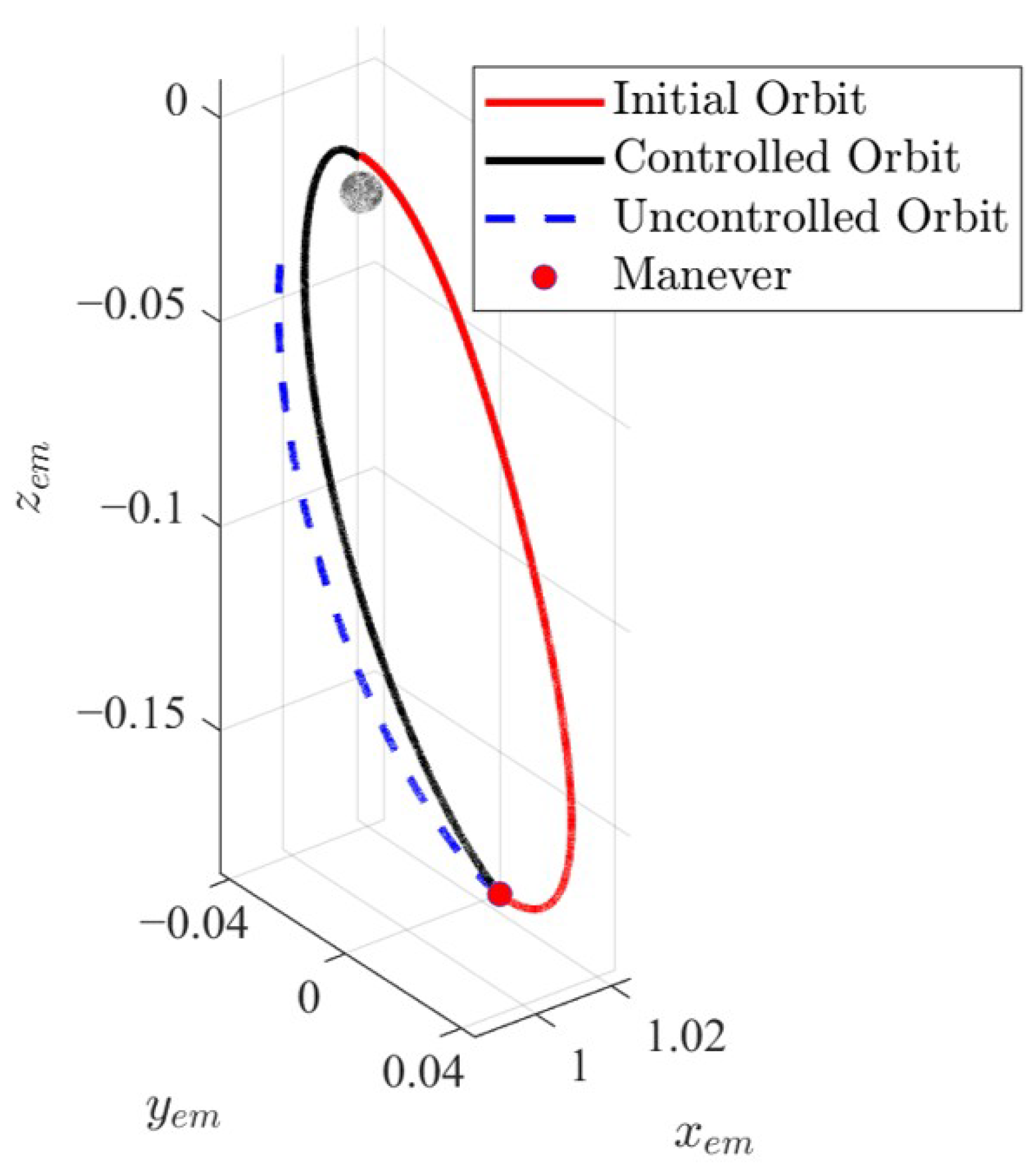
In this example, the cislunar space dynamical environment is complex, and the spacecraft in an NRHO experiences long arcs near the second primary body, leading to instability in the NRHO. Moreover, the NRHO is influenced by the gravitational forces of both the Earth and the Moon, making orbit maintenance necessary. Since the spacecraft moves faster near perilune, maneuvers are typically performed near apolune where fuel consumption is lower. Under the CRTBP model, the initial orbital data are shown in

Table 1. Initial orbit data.

Initial State	x	y	z	$\dot{\mathit{x}}$	$\dot{\mathit{y}}$	$\dot{\mathit{z}}$
Values	0.987470	0	0.009304	0.057762	1.585669	0.008737

, and the apolune orbit maintenance is shown in Figure 2. After 3.3163 days from the start of the simulation, the target spacecraft performed an impulsive maneuver with a velocity of 34.5770 m/s, completing the designated orbit maintenance mission. This was a significant impulsive maneuver, placing higher demands on the OD algorithm’s performance.

The total OD period was set to be 6 days, with a 6-min measurement interval. The initial position and velocity are given in Table 1, and the unnormalized initial error covariance matrix is

$${\mathit{P}}_{\mathit{0}}=\left[\begin{array}{cccccc}{100}^2{\mathrm{km}}^2& 0& 0& 0& 0& 0\\ 0& {100}^2{\mathrm{km}}^2& 0& 0& 0& 0\\ 0& 0& {100}^2{\mathrm{km}}^2& 0& 0& 0\\ 0& 0& 0& 1^2{\mathrm{m}}^2{\mathrm{s}}^{-2}& 0& 0\\ 0& 0& 0& 0& 1^2{\mathrm{m}}^2{\mathrm{s}}^{-2}& 0\\ 0& 0& 0& 0& 0& 1^2{\mathrm{m}}^2{\mathrm{s}}^{-2}\end{array}\right].$$

(40)

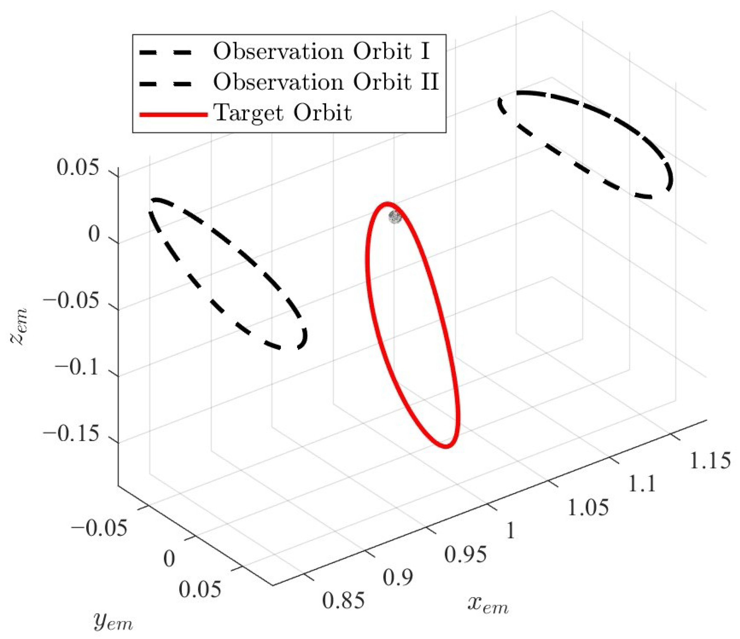
The measurement information was obtained from the observation constellation at the cislunar libration points, specifically the $L_{1,2}$ binary observation constellation in the cislunar system.

Table 2. Observation constellation configuration.

Orbit Type	Amplitude (km)	Initial Phase (deg)
L1 Halo Orbit	23,200	240
L2 PL Orbit	5000	120

gives the specific orbit types and configuration parameters of the observation constellation, and

Table 3. Initial orbit data for observation orbits.

	x	y	z	$\dot{\mathit{x}}$	$\dot{\mathit{y}}$	$\dot{\mathit{z}}$
Orbit I	0.824130	0	0.056803	0	0.167251	0
Orbit II	1.122879	0	0	0	0.164188	0

gives the initial position and velocity. Figure 3 gives a schematic of the observation and target orbits. Since the $L_{1,2}$ binary observation constellation in the cislunar system is the simplest constellation for the OD system in cislunar space, offering comprehensive coverage and a simple configuration, both angle-with-range and angle-only measurements were used as measurements to evaluate the performance of the proposed algorithm based on the observation constellation given in Figure 3.

4.2. Angle-with-Range Observation

The angle-with-range measurements of the target spacecraft obtained from the binary observation constellation sensors are given as

$${\mathit{z}}_{\mathit{k}}=\left[\begin{array}{c}arcsin\left({\displaystyle \frac{z_k-Z_{k,1}}{{\rho }_{k,1}}}\right)\\ arctan\left({\displaystyle \frac{y_k-Y_{k,1}}{x_k-X_{k,1}}}\right)\\ {\rho }_{k,1}\\ arcsin\left({\displaystyle \frac{z_k-Z_{k,2}}{{\rho }_{k,2}}}\right)\\ arctan\left({\displaystyle \frac{y_k-Y_{k,2}}{x_k-X_{k,2}}}\right)\\ {\rho }_{k,2}\end{array}\right]+{\mathit{v}}_{\mathit{k}}.$$

(41)

where ${\rho }_{k,1}={[{(x_k-X_{k,1})}^2+{(y_k-Y_{k,1})}^2+{(z_k-Z_{k,1})}^2]}^{1/2},{\rho }_{k,2}={[{(x_k-X_{k,2})}^2+{(y_k-Y_{k,2})}^2+{(z_k-Z_{k,2})}^2]}^{1/2}$. ${\left[X_{k,1}{Y}_{k,1}{Z}_{k,1}\right]}^T$ and ${\left[X_{k,2}{Y}_{k,2}{Z}_{k,2}\right]}^T$ are the position vectors of the observation spacecraft on the observation orbit I and observation orbit II, respectively. ${\mathit{v}}_{\mathit{k}}$ represents Gaussian white noise with zero mean, with covariance given as ${\mathit{R}}_k$.

$$E\left({\mathit{v}}_{\mathit{k}}{\mathit{v}}_{\mathit{k}}^T\right)={\mathit{R}}_k=\left[\begin{array}{cccccc}{\sigma }_{\theta }^2& 0& 0& 0& 0& 0\\ 0& {\sigma }_{\theta }^2& 0& 0& 0& 0\\ 0& 0& {\sigma }_{\rho }^2& 0& 0& 0\\ 0& 0& 0& {\sigma }_{\theta }^2& 0& 0\\ 0& 0& 0& 0& {\sigma }_{\theta }^2& 0\\ 0& 0& 0& 0& 0& {\sigma }_{\rho }^2\end{array}\right].$$

(42)

where the standard deviations are set to ${\sigma }_{\theta }={10}^{-6}$ for angle measurements and ${\sigma }_{\rho }=10\mathrm{m}$ for range measurements, accounting for factors such as sensor accuracy, environmental conditions, target characteristics, dynamic factors, systematic errors, and unmodeled spacecraft attitude errors.

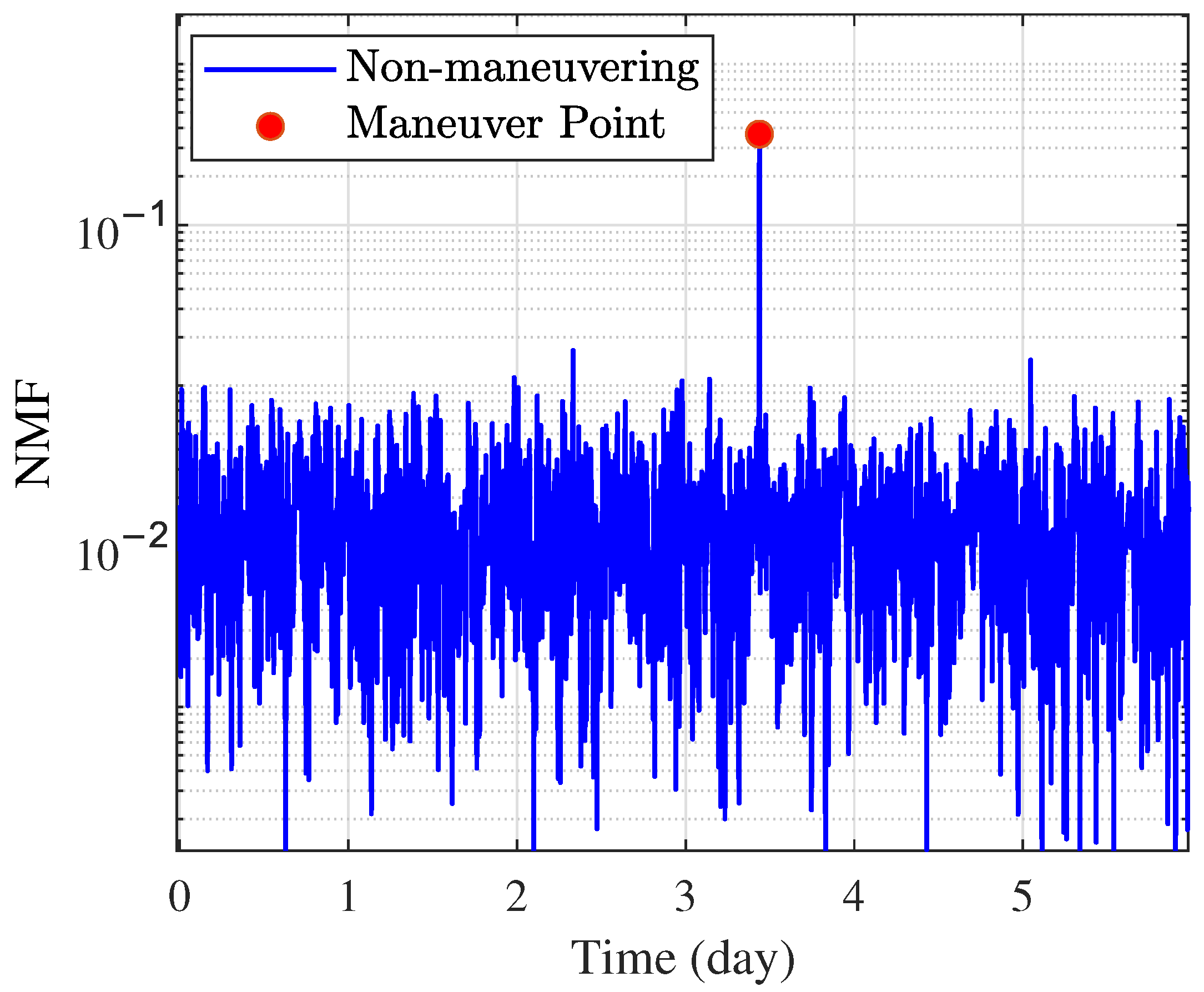
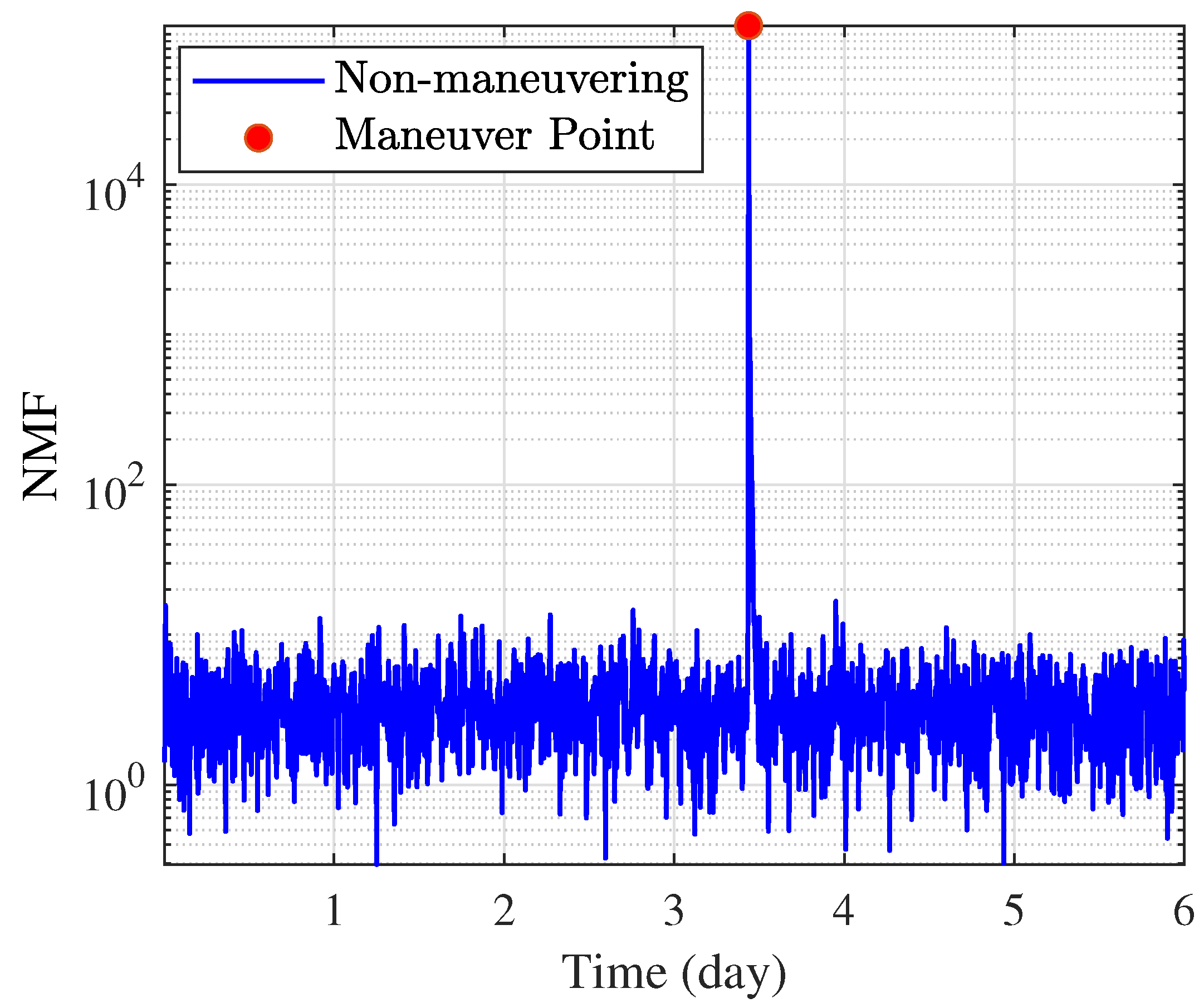
First, Monte Carlo (MC) simulations were conducted to test the OD accuracy of the proposed method when using angle-with-range measurements. Figure 4 shows the 2-norm of the NMF from 300 MC simulations. It can be observed that when the target spacecraft was not maneuvering, the NMF remained below 20, while during a maneuver, the value exceeded 10,000. This demonstrates that the proposed NMF could serve as an indicator for determining whether the target spacecraft had maneuvered. After the maneuver, with compensation for the dynamics model through state noise, the NMF did not remain at a high level, but quickly returned to the same magnitude as before the maneuver, verifying the effectiveness of the proposed algorithm. 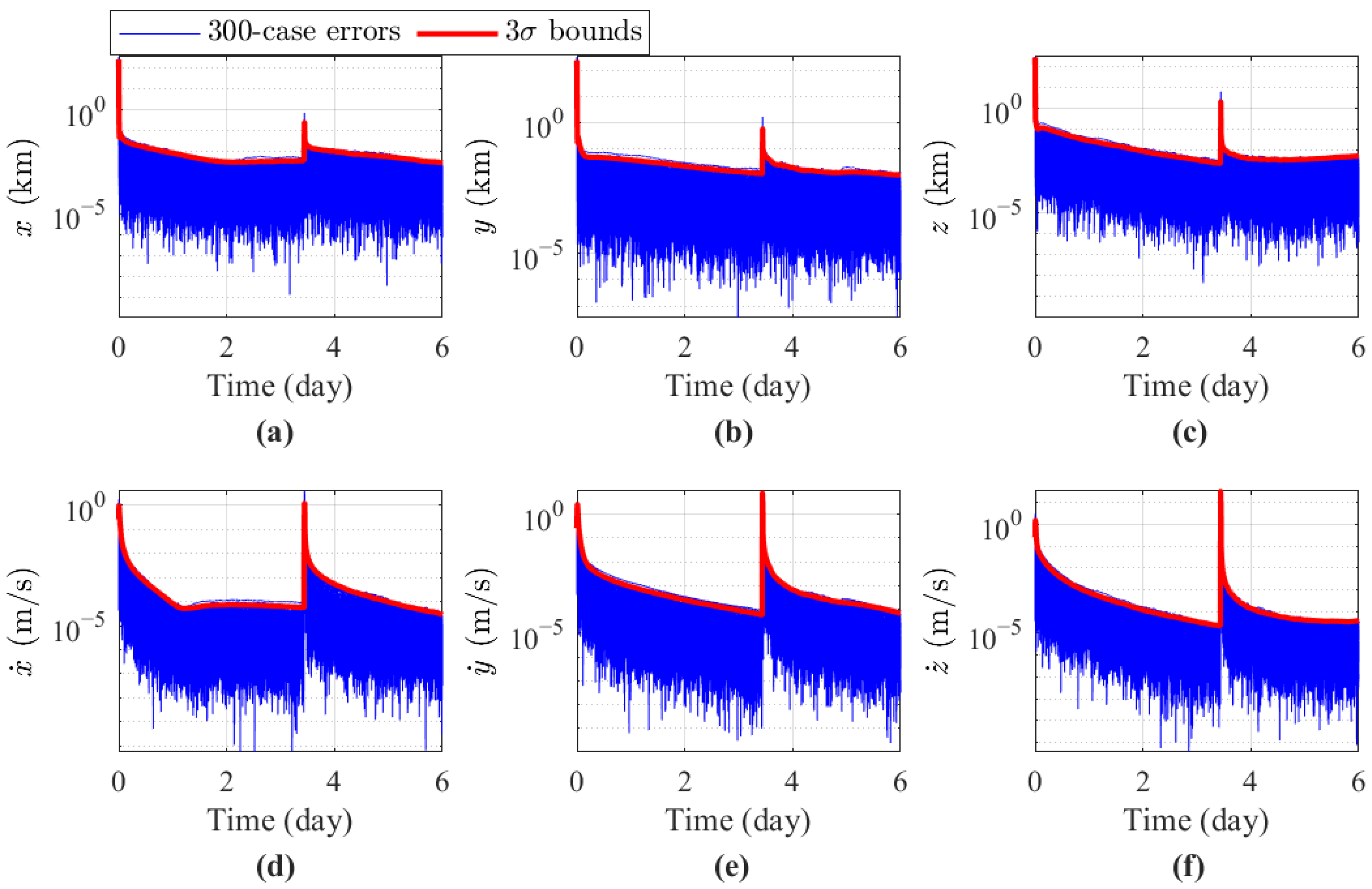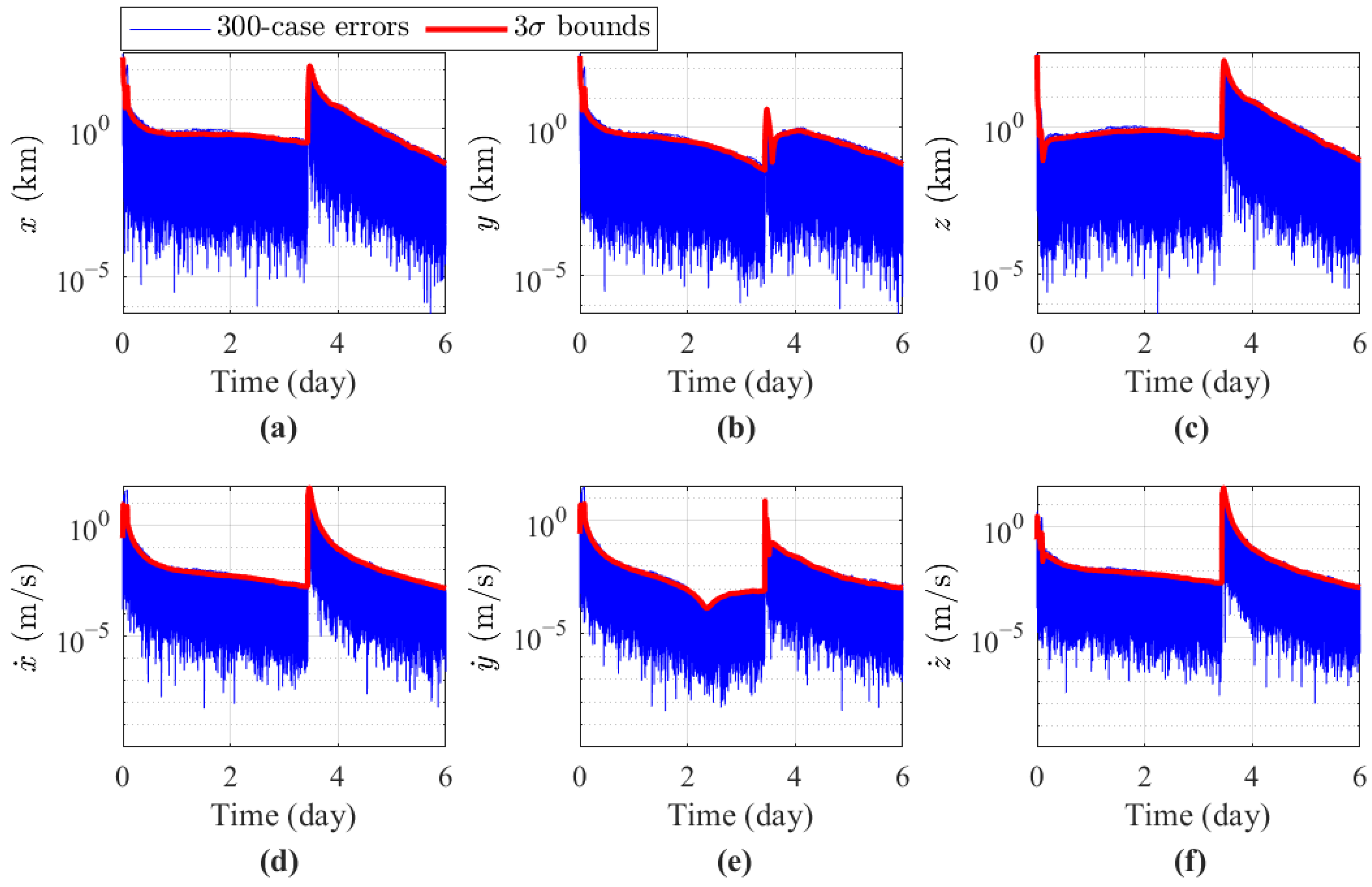Figure 5 shows the estimation errors of the three-axis velocity and three-axis position for 300 MC simulations, with the red boundary indicating the $3\sigma$ envelope of the estimation errors, and the blue lines representing the error for each OD run.

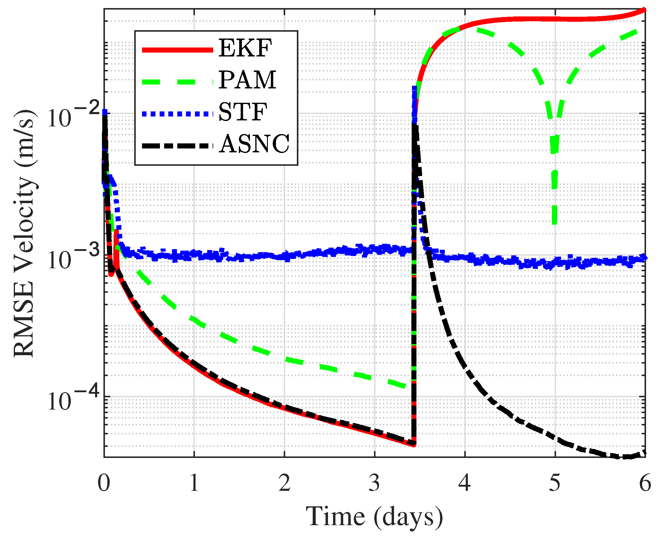
Then, the performance of the proposed algorithm was compared with that of three representative algorithms for maneuverable spacecraft: EKF, STF, and PAM. EKF is a widely used nonlinear filtering method that linearizes the system dynamics and measurement model. It exhibits a certain robustness and can handle disturbances to some extent. Next, STF, a Kalman filter-based algorithm, relies on the orthogonalization principle of residuals to estimate the state of maneuverable spacecraft. In this scenario, the forgetting factor was set to 0.95, and since there was no prior information on the maneuver magnitude and epoch, all selected coefficients were set to 1. Finally, the proposed algorithm was compared with PAM for OD of maneuverable spacecraft. PAM models the maneuvering portion of the spacecraft as an estimated state vector and uses polynomial fitting to handle unknown maneuvers. In this case, since the unknown maneuver was impulsive, the polynomial was set to 0th order, retaining only the constant term, and the initial maneuver magnitude was set to 0. By including EKF in the comparison, we aimed to provide insights into how traditional nonlinear filtering methods perform in the context of impulsive maneuvers and highlight the advantages of the proposed approach.

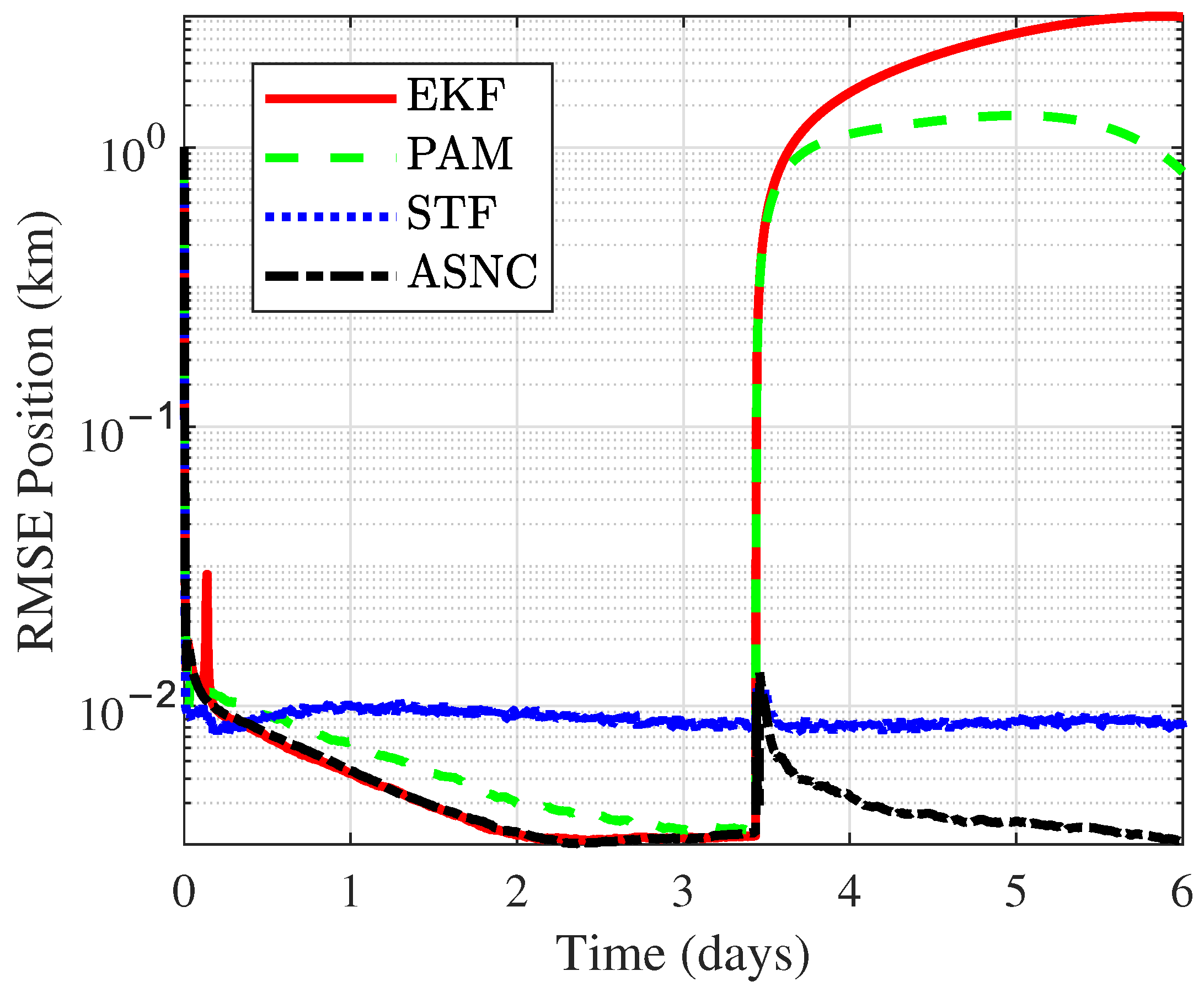
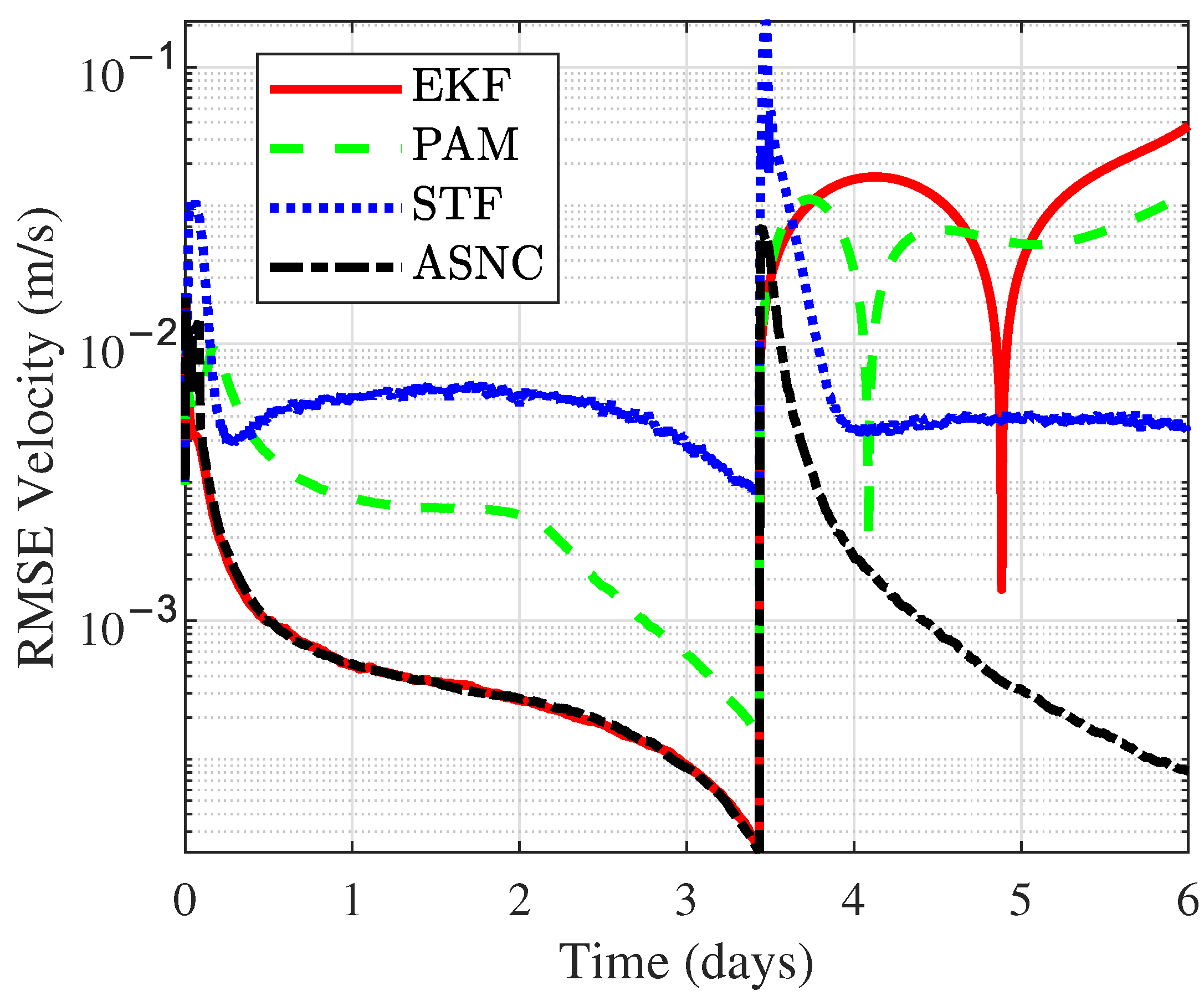
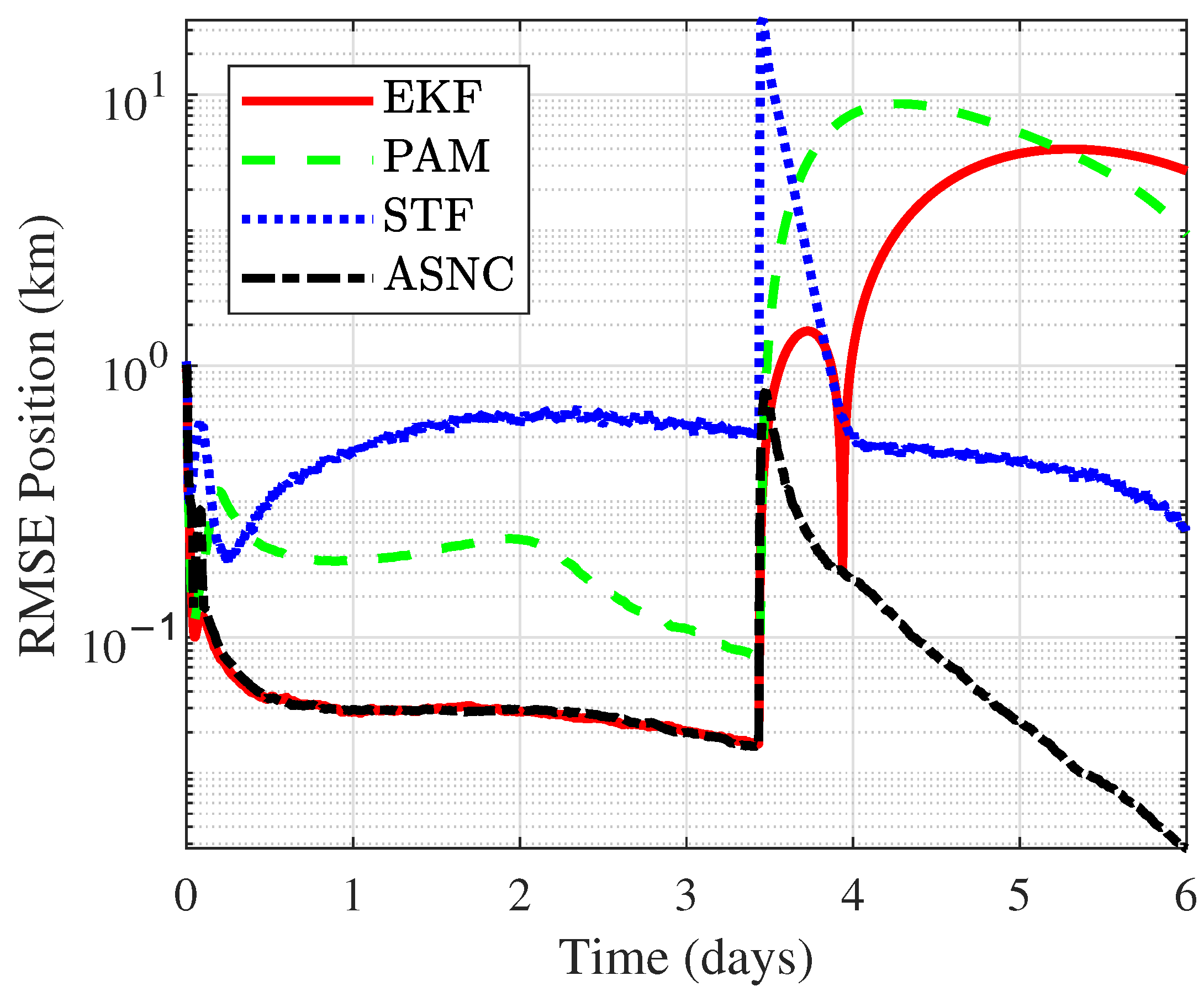
Figure 6 compares the Root Mean Square Error (RMSE) of velocity for the three methods over 300 Monte Carlo simulations, while Figure 7 compares the RMSE of position.

Table 4. Comparison of RMSE position for angle-with-range observation (km, 300 MC simulations).

Day	1	2	3	Maneuver Epoch	4	5	6
EKF	0.00338	0.00125	0.00110	2.80381	247.278	653.685	864.118
PAM	0.00546	0.00210	0.00129	9.15143	124.366	169.328	69.0519
STF	0.01014	0.00888	0.00738	0.01312	0.00748	0.00807	0.00749
ASNC	0.00288	0.00125	0.00104	0.01486	0.00238	0.00151	0.00090

and

Table 5. Comparison of RMSE velocity for angle-with-range observation (m/s, 300 MC simulations).

Day	1	2	3	Maneuver Epoch	4	5	6
EKF	0.00027	6.79 $\times {10}^{-5}$	3.03 $\times {10}^{-5}$	1.1981	16.869	21.422	29.164
PAM	0.00122	0.00034	0.00018	1.51279	16.7973	0.02067	15.8551
STF	0.01011	0.00838	0.01284	2.52556	0.00847	0.00757	0.00889
ASNC	0.00030	7.20 $\times {10}^{-5}$	2.99 $\times {10}^{-5}$	0.92771	2.74 $\times {10}^{-4}$	2.63 $\times {10}^{-5}$	1.66 $\times {10}^{-5}$

provide detailed numerical comparisons of the RMSE for position and velocity, respectively, under angle-with-range measurements. When no maneuver occurred, the ASNC algorithm achieved the smallest OD error, with velocity RMSE on the order of ${10}^{-5}\mathrm{m}/\mathrm{s}$ and position RMSE on the order of ${10}^{-3}\mathrm{km}$. The PAM algorithm showed the second-best accuracy, with its velocity and position RMSE about one order of magnitude higher than ASNC, while the STF algorithm yielded the largest position and velocity errors. This was due to STF’s lack of prior information on the maneuver, making it difficult to configure the filter for more precise OD. The ASNC algorithm used the NMF to detect spacecraft maneuvers in real time, ensuring that the state noise was set to zero when no maneuver occurred, thus maintaining maximum accuracy, without filter divergence. When a maneuver occurred, PAM diverged quickly, leading to significant estimation errors, as it struggled to approximate the state transitions caused by spacecraft impulsive maneuvers using polynomial fitting. Meanwhile, the proposed ASNC algorithm outperformed STF in maneuver scenarios by utilizing Position State Noise Estimation via Match and Velocity State Noise Estimation via Inverse Mapping, ensuring the filter obtained the optimal state noise covariance matrix for high-precision OD during maneuvers.

Figure 6 compares the Root Mean Square Error (RMSE) of velocity for the four methods over 300 Monte Carlo simulations, while Figure 7 compares the RMSE of position. Table 4 and Table 5 provide detailed numerical comparisons of the RMSE for position and velocity, respectively, under angle-with-range measurements. When no maneuver occurred, both the ASNC algorithm and the EKF achieved the smallest OD error, with the velocity RMSE on the order of ${10}^{-5}\mathrm{m}/\mathrm{s}$ and the position RMSE on the order of ${10}^{-3}\mathrm{km}$. The PAM algorithm showed the second-best accuracy, with its velocity RMSE about one order of magnitude higher than ASNC and its position RMSE approximately twice that of ASNC. In contrast, the STF algorithm yielded the largest position and velocity errors. This was due to STF’s lack of prior information on the maneuver, making it difficult to configure the filter for more precise OD. The ASNC algorithm used the NMF to detect spacecraft maneuvers in real time, ensuring that the state noise was set to zero when no maneuver occurred, thus maintaining the maximum accuracy, without filter divergence. When a maneuver occurred, both PAM and EKF diverged quickly, leading to significant estimation errors. PAM struggled to approximate the state transitions caused by impulsive maneuvers using polynomial fitting, while EKF exhibited limited robustness in handling impulsive maneuvers. In contrast, the proposed ASNC algorithm outperformed STF in maneuver scenarios by utilizing Position State Noise Estimation via Match and Velocity State Noise Estimation via Inverse Mapping, ensuring the filter obtained the optimal state noise covariance matrix for high-precision OD during maneuvers.

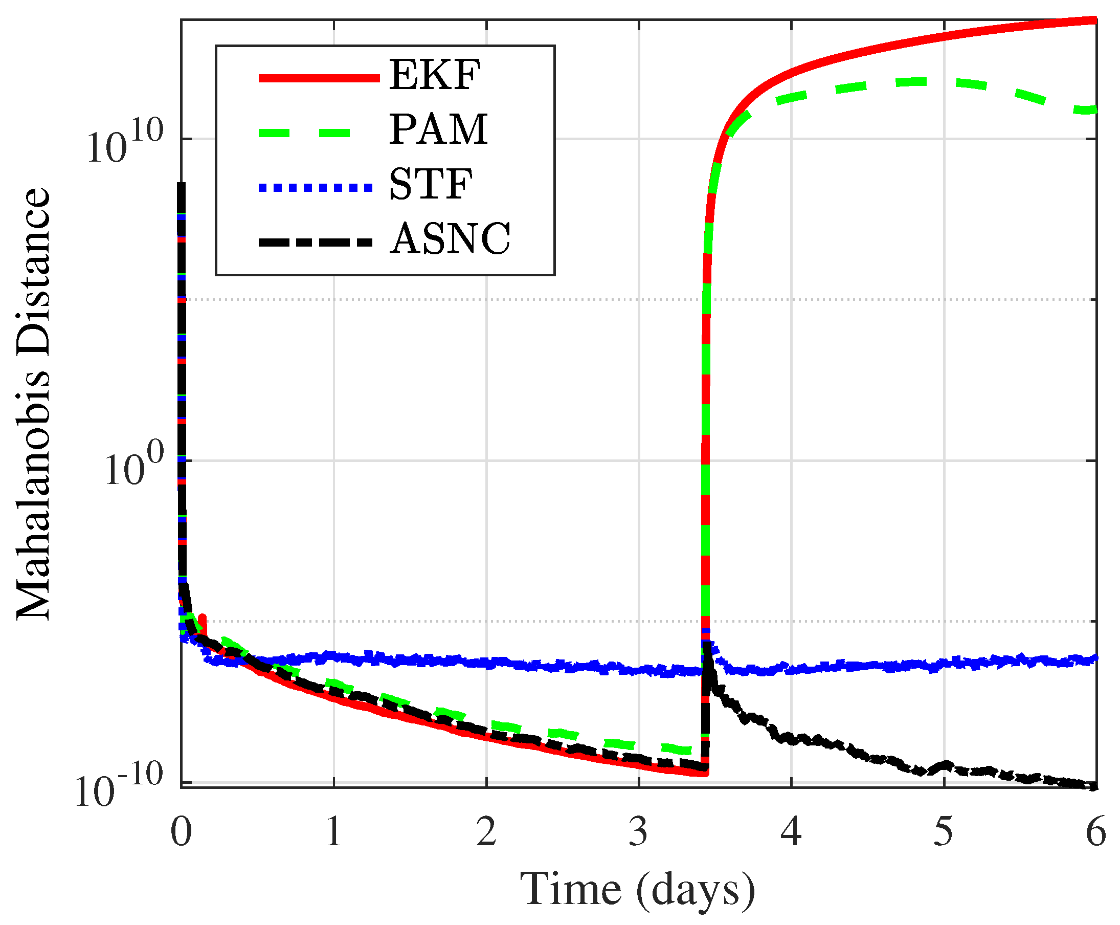
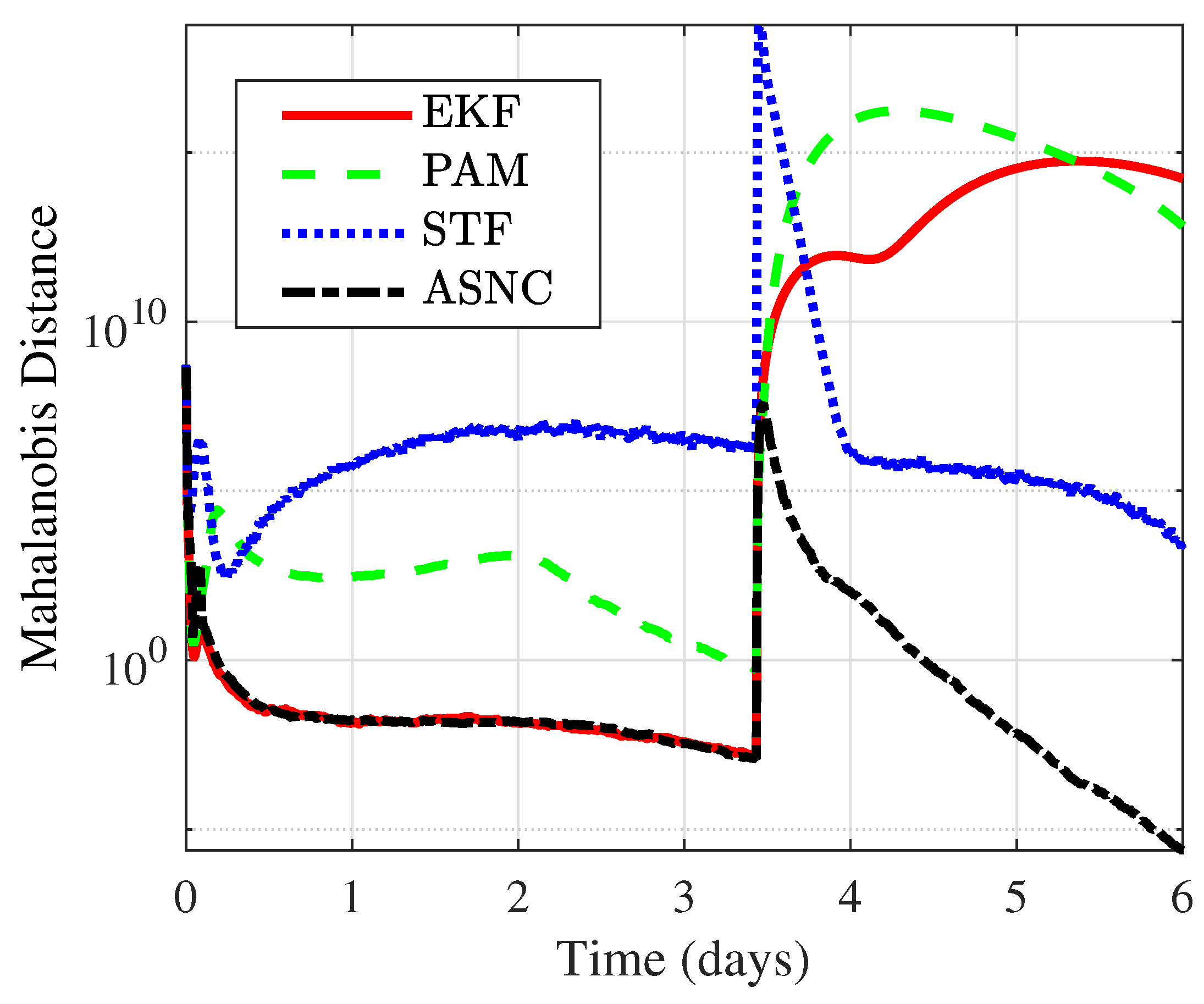
Next, the uncertainty of OD was measured using the Mahalanobis distance (MD), which is an important quantitative metric for evaluating algorithm uncertainty [18]. The Mahalanobis distance not only reflects the difference between estimated and actual positions but also takes into account the covariance in different directions, providing a more comprehensive assessment of estimation uncertainty. Unlike Euclidean distance (ED), MD eliminates the influence of different scales among variables, allowing errors in different measurement dimensions to be evaluated using the same standard. Therefore, using MD provided a more accurate evaluation of the uncertainty of the OD algorithm. The calculation formula for MD is shown in Equation (43)

$$D_M=\sqrt{{(\widehat{\mathit{x}}-\mathit{\mu })}^T{\mathbf{\Sigma }}^{-1}(\widehat{\mathit{x}}-\mathit{\mu })}.$$

(43)

where $\widehat{\mathit{x}}$ is the estimated state vector, $\mathit{\mu }$ is the true state vector, and $\mathbf{\Sigma }$ is the covariance matrix of the estimated state vector. In this example, $\widehat{\mathit{x}}$ was replaced by the mean value from 300 MC simulations.

Figure 8 compares the MD of the four methods over 300 MC simulations, and

Table 6. Comparison of MD for angle-with-range observation (300 MC simulations).

Day	1	2	3	Maneuver Epoch	4	5	6
EKF	$4.31\times {10}^{-8}$	$2.60\times {10}^{-9}$	$2.98\times {10}^{-10}$	$2.40\times {10}^6$	$1.15\times {10}^{12}$	$1.51\times {10}^{14}$	$4.85\times {10}^{14}$
PAM	$1.24\times {10}^{-7}$	$6.84\times {10}^{-9}$	$1.39\times {10}^{-9}$	$5.80\times {10}^5$	$1.90\times {10}^{11}$	$5.87\times {10}^{11}$	$8.07\times {10}^{10}$
STF	$7.86\times {10}^{-7}$	$6.27\times {10}^{-7}$	$2.83\times {10}^{-7}$	$6.18\times {10}^{-6}$	$2.81\times {10}^{-7}$	$4.98\times {10}^{-7}$	$7.49\times {10}^{-7}$
ASNC	$5.70\times {10}^{-8}$	$3.08\times {10}^{-9}$	$3.09\times {10}^{-10}$	$2.30\times {10}^{-6}$	$3.75\times {10}^{-9}$	$2.55\times {10}^{-10}$	$4.95\times {10}^{-11}$

provides a detailed numerical comparison of MD under angle-with-range measurements. Similarly to for the RMSE comparison, the ASNC algorithm outperformed the other algorithms in terms of MD, both in non-maneuvering and maneuvering scenarios.

Finally,

Table 7. Time consumption comparison for different algorithms using angle-with-range observation (300 MC simulations).

	Min (s)	Max (s)	Sum (s)	Average (s)
PAM	0.8136	7.239	279.6	0.9320
STF	0.4126	10.56	159.7	0.5323
ASNC	0.3996	6.948	143.6	0.4787

compares the average single run time and total time consumption for 300 MC simulations across the three algorithms (EKF is excluded from the comparison). PAM exhibited the longest computation time, followed by STF, while the proposed algorithm demonstrated the smallest time consumption. This efficiency was achieved because the proposed algorithm modeled the state noise as a piecewise function based on the NMF, effectively handling both maneuvering and non-maneuvering phases of the impulsive maneuver spacecraft. The computationally intensive processes of Position State Noise Estimation via Match and Velocity State Noise Estimation via Inverse Mapping were only activated during maneuvers. As a result, the proposed algorithm achieved the shortest computation time, reducing the time consumption by 11.00% compared to STF and by 94.50% compared to PAM.

4.3. Angle-Only Observation

In this section, angle-only measurements from a single observation satellite (Observation Orbit I) were used. Compared to angle-with-range observation, angle-only observation has fewer observation dimensions, resulting in sparser observational data. This type of measurement provided more limited spatial positioning information, which imposed higher demands on the OD algorithm. Additionally, validating the proposed algorithm under single-satellite observation conditions helped extend its applicability to near-Earth rendezvous and proximity operations, particularly for uncooperative target spacecraft. The angle measurements of the target spacecraft are given as

$${\mathit{z}}_k=\left[\begin{array}{c}arcsin\left({\displaystyle \frac{z_k-Z_{k,1}}{{\rho }_{k,1}}}\right)\\ arctan\left({\displaystyle \frac{y_k-Y_{k,1}}{x_k-X_{k,1}}}\right)\end{array}\right]+{\mathit{v}}_k.$$

(44)

where ${\rho }_{k,1}={\left[{(x_k-X_{k,1})}^2+{(y_k-Y_{k,1})}^2+{(z_k-Z_{k,1})}^2\right]}^{1/2}$ represents the distance between the target spacecraft and the observation spacecraft on Observation Orbit I. ${\mathit{v}}_k$ represents Gaussian white noise with zero mean, with covariance given as ${\mathit{R}}_k$

$$E\left({\mathit{v}}_{\mathit{k}}{\mathit{v}}_{\mathit{k}}^T\right)={\mathit{R}}_k=\left[\begin{array}{cc}{\sigma }_{\theta }^2& 0\\ 0& {\sigma }_{\theta }^2\end{array}\right].$$

(45)

where the standard deviation was set to ${\sigma }_{\theta }={10}^{-6}$ for angle measurements, accounting for factors such as sensor accuracy, environmental conditions, target characteristics, dynamic factors, systematic errors, and unmodeled spacecraft attitude errors.

Similarly to the analysis process for angle-with-range observations, MC simulations were first conducted to test the OD accuracy of the proposed method when using angle-only measurements. Figure 9 shows the 2-norm of the NMF from 300 MC simulations. It can be observed that when the target spacecraft was not maneuvering, the NMF remained below 50, while during a maneuver, its value exceeded 100. This demonstrates that the proposed NMF could also be used to determine whether the target spacecraft had maneuvered under angle-only observations. After the maneuver, the NMF quickly returned to the same magnitude as before the maneuver, verifying the effectiveness of the proposed algorithm for angle-only measurements. Figure 10 shows the estimation errors of the three-axis velocity and three-axis position for 300 MC simulations, with the red line indicating the $3\sigma$ bound of the estimation errors, and the blue lines representing the error for each OD run.

As in the case of the angle-with-range observations, the proposed algorithm was compared with EKF, STF, and PAM: The forgetting factor for STF was set to 0.95, and all selected coefficients were set to 1. In PAM, because the unknown maneuver was impulsive, the polynomial was set to 0th order, retaining only the constant term, and the initial maneuver magnitude was set to 0.

Figure 11 compares the RMSE velocity of the four methods over 300 MC simulations, and Figure 12 compares the RMSE position.

Table 8. Comparison of RMSE position for angle-only observation (km, 300 MC simulations).

Day	1	2	3	Maneuver Epoch	4	5	6
EKF	0.29180	0.29145	0.20344	38.8259	103.52	3670.29	2768.11
PAM	3.70628	5.28096	1.16958	170.42	7161.43	5294.41	1026.24
STF	22.9147	39.2144	39.549	34,121.7	30.0153	19.8122	6.72683
ASNC	0.29180	0.295532	0.204662	22.0366	2.65665	0.23828	0.02977

and

Table 9. Comparison of RMSE velocity for angle-only observation (m/s, 300 MC simulations).

Day	1	2	3	Maneuver Epoch	4	5	6
EKF	0.00490	0.002756	0.00086	7.65491	15.4147	3.31521	37.2656
PAM	0.07654	0.05790	0.00575	9.9199	3.52421	5.31253	12.3776
STF	0.434281	0.405548	0.192661	208.991	0.241143	0.2888	0.254293
ASNC	0.00485	0.00275	0.00093	6.40077	0.03016	0.003225	0.000824

provide detailed numerical comparisons of the RMSE for position and velocity, respectively, under angle-only measurements. In the absence of maneuvers, the proposed ASNC algorithm and the EKF achieved the highest OD accuracy, with RMSE velocity on the order of ${10}^{-3}\mathrm{m}/\mathrm{s}$ and RMSE position on the order of ${10}^{-1}\mathrm{km}$. PAM achieved a better position and velocity accuracy than STF, but both were at least one order of magnitude lower in accuracy compared to ASNC and EKF. When a maneuver occurred, the proposed ASNC algorithm achieved an RMSE position of 22.0366 km and an RMSE velocity of 6.40077 m/s, and then quickly converged to the same accuracy as before the maneuver, with RMSE velocity on the order of ${10}^{-3}\mathrm{m}/\mathrm{s}$ and RMSE position on the order of ${10}^{-1}\mathrm{km}$. During the maneuver, both PAM and EKF diverged rapidly, leading to significant estimation errors, while STF converged slowly to an accuracy comparable to that before the maneuver. Under under-determined conditions, ASNC maximized the processing of the state noise covariance matrix, ensuring convergence, while achieving high OD accuracy.

Figure 13 compares the MD of the four methods over 300 MC simulations under angle-only measurements, and

Table 10. Comparison of MD for angle-only observation (300 MC simulations).

Day	1	2	3	Maneuver Epoch	4	5	6
EKF	$1.60\times {10}^{-2}$	$1.49\times {10}^{-2}$	$3.37\times {10}^{-3}$	$6.29\times {10}^8$	$8.22\times {10}^{12}$	$3.36\times {10}^{14}$	$1.80\times {10}^{14}$
PAM	$2.80\times {10}^2$	$1.20\times {10}^3$	$3.89\times {10}^1$	$1.80\times {10}^{12}$	$8.19\times {10}^{15}$	$2.65\times {10}^{15}$	$6.95\times {10}^{11}$
STF	$6.09\times {10}^5$	$5.34\times {10}^6$	$3.62\times {10}^6$	$4.92\times {10}^{18}$	$1.44\times {10}^6$	$2.89\times {10}^5$	$2.33\times {10}^3$
ASNC	$1.60\times {10}^{-2}$	$1.49\times {10}^{-2}$	$3.37\times {10}^{-3}$	$4.11\times {10}^6$	$1.06\times {10}^2$	$7.22\times {10}^{-3}$	$2.45\times {10}^{-6}$

provides a detailed numerical comparison of MD. Unlike the angle-with-range measurements, the OD performance of all four methods declined. Before the maneuver, ASNC and EKF achieved the highest OD accuracy, with an MD on the order of ${10}^{-3}$. After the maneuver, the MDs of EKF, STF, and PAM reached the orders of ${10}^{15}$, ${10}^{12}$, and ${10}^6$, respectively, while ASNC maintained the lowest MD, on the order of ${10}^{-3}$. Therefore, even under angle-only measurements, ASNC still demonstrated the best OD performance.

Table 11. Time consumption comparison for different algorithms using angle-only observation (300 MC simulations).

	Min (s)	Max (s)	Sum (s)	Average (s)
PAM	0.7386	4.9843	593.34	1.9778
STF	0.3781	0.5394	126.76	0.4225
ASNC	0.3638	0.4929	112.19	0.3740

provides a comparison of the single run and total time consumption for 300 MC simulations using the three different algorithms (EKF is excluded from the comparison). PAM had the longest time consumption, while the STF and the ASNC algorithm had a similar time consumption, with the proposed algorithm consuming slightly less. The ASNC algorithm still achieved the highest computational efficiency when using angle-only information as the measurement, performing on par with STF (12.97% more efficient) and significantly outperforming PAM (428.82% improvement).

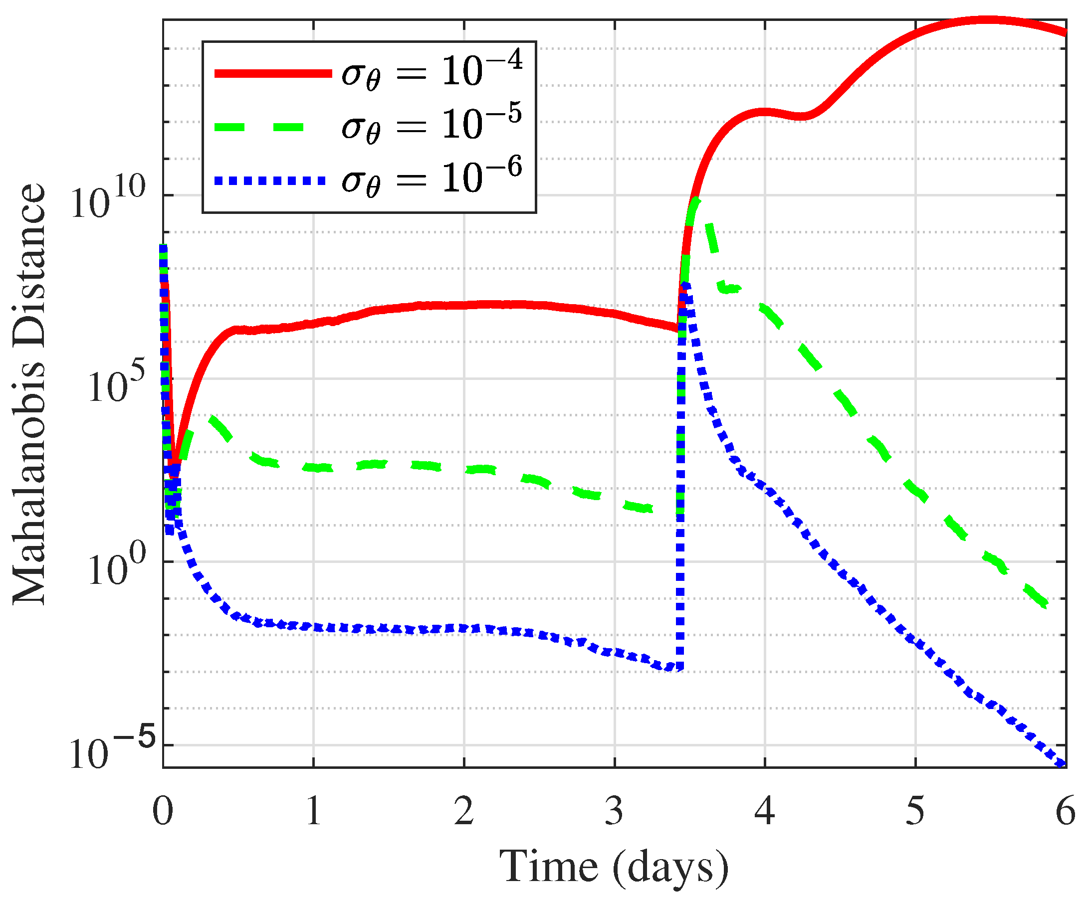
Figure 14 compares the MD of the different measurement noise levels in 300 MC simulations under angle-only measurements. As can be seen from the figure, in the absence of maneuvers, the OD accuracy decreased as the measurement noise increased. When a maneuver occurred, the OD results diverged if the noise exceeded a certain threshold (${\sigma }_{\theta }={10}^{-4}$). Therefore, lower measurement noise led to stronger robustness and higher accuracy, and the proposed algorithm was relatively sensitive to noise.

5. Conclusions

This paper proposed an adaptive state noise compensation (ASNC) method for orbit determination (OD) of impulsively maneuverable spacecraft. The method adaptively compensates for inaccurately modeled dynamics through position state noise estimation through match and velocity state noise estimation via inverse mapping. The proposed approach was applied to the highly nonlinear dynamics scenario of the Earth–Moon three-body system, and its OD performance was tested using both angle-with-range and angle-only measurements. The simulation results demonstrated that the proposed NMF effectively reflected the spacecraft’s maneuvering status, with the NMF differing by at least 2 orders of magnitude between maneuver epochs and non-maneuver epochs. Next, the ASNC algorithm was compared with other algorithms in terms of performance. The results show that, in the case of angle-with-range (over-determined) measurements, the proposed algorithm achieved the lowest OD errors, with its OD error being at least 1 order of magnitude lower than the comparison algorithms. In the case of angle-only (under-determined) measurements, the comparison algorithms diverged, while the proposed algorithm demonstrated optimal convergence and robustness. Finally, an efficiency comparison revealed that the ASNC algorithm outperformed both STF and PAM in computational performance, with a reduction in computation time of at least 11%.

The proposed method assumes maneuvers occur between observations, but in practice, maneuvers may last and overlap with observations. Future work will address this by improving the algorithm, such as introducing dynamic maneuver models or designing adaptive filtering methods, to better handle observations during maneuvers and enhance the method’s applicability and robustness. Additionally, we plan to compare the proposed method with machine-learning-based approaches for orbit determination.