1. Introduction
Cold chain temperature management is crucial for maintaining the quality, safety, and shelf life of temperature-sensitive products across various industries, including pharmaceuticals, food, and biochemicals. The critical role of cold chain management is highlighted by [
1], who found that improper temperature control during extended transportation results in about 40% value loss for fruits and vegetables.
Temperature management in cold storage rooms is crucial for maintaining product quality and reducing energy consumption. There are several critical weak points in cold chains: precooling operations, ground transportation operations, retail display, and consumer handling [
2]. Studies show temperature variations can be as high as 10 °C during transport, with vulnerability during loading and unloading operations [
3]. Notably, consumer handling represents the weakest link, with domestic refrigerator temperatures often exceeding recommended levels by 2–3 °C [
4].
As noticed from the above presented critical weak points, proper temperature management could greatly mitigate the risk of exceeding the required temperature range for transported goods. Proper temperature management largely depends on reliable methodologies to accurately measure and predict cold storage room temperature. CFD has proven valuable for optimizing cooling equipment placement. CFD is a method that uses computer simulations to predict and analyze fluid flow and heat transfer by solving mathematical equations across a discretized domain, enabling engineers to understand complex fluid behavior in various systems [
5]. In their work, Ref. [
6] validated the accuracy of 3D CFD modeling for predicting temperature distributions in refrigerated containers through experimental studies. Meanwhile, Ref. [
7] used CFD models to study airflow in cold storage apple crates, finding that wider spacing between stacks improves cooling efficiency by 25.2% compared to conventional arrangements, while maintaining more uniform temperatures throughout. A 3D CFD model for predicting temperature distribution in cold storage rooms using ultrasonic humidifiers was validated by Ref. [
6], achieving accuracy with limited error for air velocity and temperature measurements in experiment validation. Several research works have highlighted the importance of proper airflow design in maintaining uniform temperature distribution and advanced phase change material to improve energy efficiency [
8,
9]. In Ref. [
10], the authors utilized CFD simulations to analyze the impact of door openings on temperature fluctuations in cold storage rooms. Their research revealed that traditional CFD models, while accurate, required significant computational resources and time for complex scenarios.
CFD modeling of cold storage rooms is constrained by high computational costs, especially for large facilities and complex operations like door openings. Model validation challenges arise from limited experimental data, while accuracy depends heavily on boundary condition assumptions and heat load estimations [
11]. The models struggle with rapid transient events and complex turbulent flows, and the detailed geometric requirements for products and equipment make mesh generation demanding, often requiring simplifications that can affect prediction accuracy of temperature and airflow patterns.
Recent years have seen an increase in the application of machine learning techniques to cold chain management. The authors of [
12] developed a machine learning model combining optimal control and k-means clustering to manage cold storage temperatures, identifying optimal storage conditions between −0.87 °C and 3.31 °C for preserving perishable foods. Their model significantly reduced computational time compared to traditional CFD approaches. By using a machine learning model, [
13] predicted cold chain temperatures in real-time, although accuracy depends on the training data quality. Experimental data provide 20–40% better results than synthetic data, which can lead to overfitting. The study recommends optimizing sensor placement and improving thermal models rather than increasing data volume. The authors of [
14] developed a machine learning pipeline to forecast energy usage, temperature, and humidity in food cold storage facilities one week in advance. The research reveals that Random Forest models achieved the best electricity consumption predictions when using real-world data from two facilities, and [
15] developed a deep learning model combining Convolutional Neural Network (CNN) and Long Short-Term Memory (LSTM) architecture with transfer learning to predict egg freshness during cold storage, using nondestructive weight loss measurements from various temperature conditions. The model achieved superior accuracy compared to traditional methods like Random Forest, enabling effective real-time quality monitoring in cold chain environments. However, as noted by [
2], challenges remain in standardizing these approaches across different storage facility configurations and product types.
While the advancement of machine learning greatly improves temperature management for cold storage, machine learning in cold storage temperature studies is limited by the need for extensive training data and struggles with generalization across different facility layouts. Model accuracy depends heavily on data quality, while real-time implementation requires robust sensor networks and processing capabilities. The “black box” nature of ML models makes physical validation challenging, and they may fail to handle unexpected scenarios not present in training data.
2. Methodology
In the present study, it is intended to create an integration of CFD and machine learning to create a powerful tool that enhances both computational efficiency and accuracy in the prediction of temperature for cold storage rooms. This hybrid approach reduces computation time by using machine learning models trained on previous CFD simulations, enabling rapid prediction and optimization. While machine learning models require less computational power than full CFD simulations, they can improve prediction accuracy to handle the complex thermal and fluid dynamics systems of cold storage more efficiently.
In the present study, a full-scale 3D CFD model is firstly developed by referring to the recent research of [
16], in which the authors systematically studied temperature distribution inside a refrigerated container. The baseline results are compared and validated with the experimental measurements. Afterwards, more than 200 cases with varying process conditions were run to be used by developing machine learning models. The machine learning models predict the temperature distribution of the cold storage boxes in the container to provide comprehensive guidance for temperature management by considering different process conditions in food and vaccine cold supply chain management.
2.1. Baseline Validation
Figure 1 shows the schematic view of the cold container used in the baseline study of the present CFD model. The container is 11.65 m long, 2.28 m in width, and 2.56 m in height. Cold air is supplied from a refrigeration unit and distributed throughout the whole container and returned from the grille on the side. There are a total of 10 arrays of boxes that contain perishable frozen food or vaccines that are placed along the length direction, which are numbered from 1 to 10 from the cold air inlet location to the door (whose dimensions are 0.5 m × 0.5 m × 0.54 m); see details in
Figure 1a. Thus, by referring to
Figure 1b, one can read that the computational domain spans 0–11.65 m in the x direction for domain length, 0–2.28 m in the y direction for domain width, and 0–2.56 m in the z direction for domain height. The cold temperature management of the container is largely dependent on how well the container is insulated, and
Figure 1b shows the insulation material layers on the outside of the container. Both the top cover and side wall are insulated with polyurethane foam (PUR), whose thicknesses are 13.6 cm and 6.6 cm, respectively.
The cold room exhibits symmetry along its longitudinal axis, which allows the CFD model to leverage this symmetrical nature in our modeling approach. By taking advantage of this symmetry, we can significantly reduce computational requirements while maintaining model accuracy. This symmetrical domain assumption is justified by the uniform arrangement of storage boxes and the balanced distribution of cold air from the refrigeration unit.
The developed CFD model performs a steady-state simulation. Turbulent flow is generated by the supplying cold air; the unit is modeled by a two-equation Reynold Average Navior–Stokes (RANS) model and Realizable k-ε model, as they provide better prediction of flow recirculation in confined spaces [
17]. By referring to the experiment condition in [
16], the boundary condition used in the baseline CFD model has “velocity inlet” at the cold air inlet, which is m/s at −37.3 °C and provides a total cold air volumetric flowrate of 0.38
. The thermal conductivity of the PUR insulation material is 0.0245 W/(m·K), both for the top cover and side walls, as shown in
Figure 1b. As described above, the CFD model used “symmetry” boundary conditions so that the computational domain with half of the total width, shown in
Figure 1b, is modeled.
The authors of Ref. [
16] used thermocouples to measure multiple locations, including 6 data points for temperature distribution in the container and 1 data point for the returning air grille. In the above baseline study, a total of ~68,3900 tetrahedral meshes were used in the CFD model, which is based upon an independent mesh study to ensure this solution (e.g., temperature at the thermocouple measurement locations does not change with a further increase of mesh number).
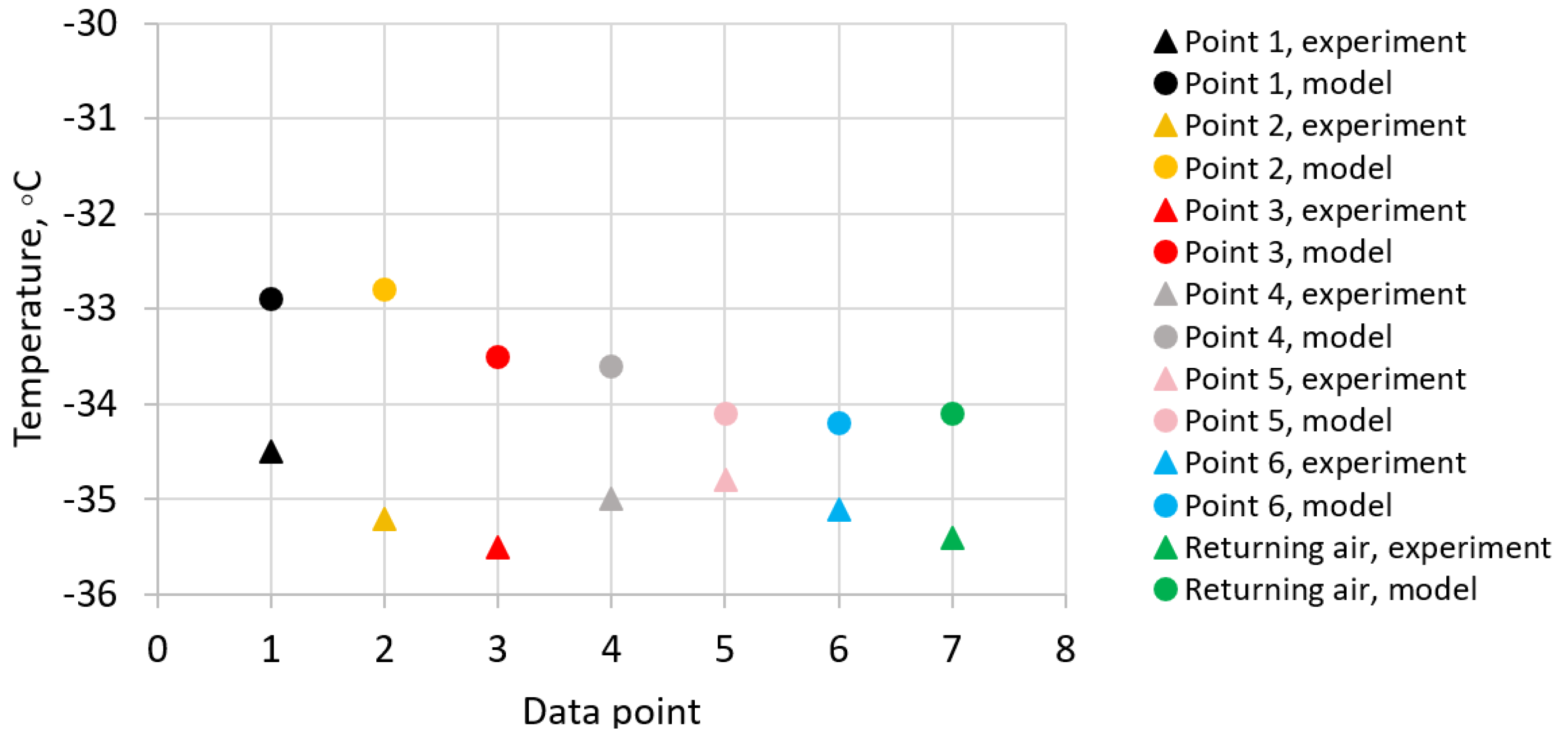
The comparison between the experiment and the present model is shown in
Figure 2. The numerical model systematically slightly overpredicts temperatures by 2–3 °C compared to experimental measurements across all data points. However, the model accurately captures the overall temperature distribution from the experiment, showing good agreement between the present CFD model and the experimental measurements.
2.2. CFD Model Results Analysis
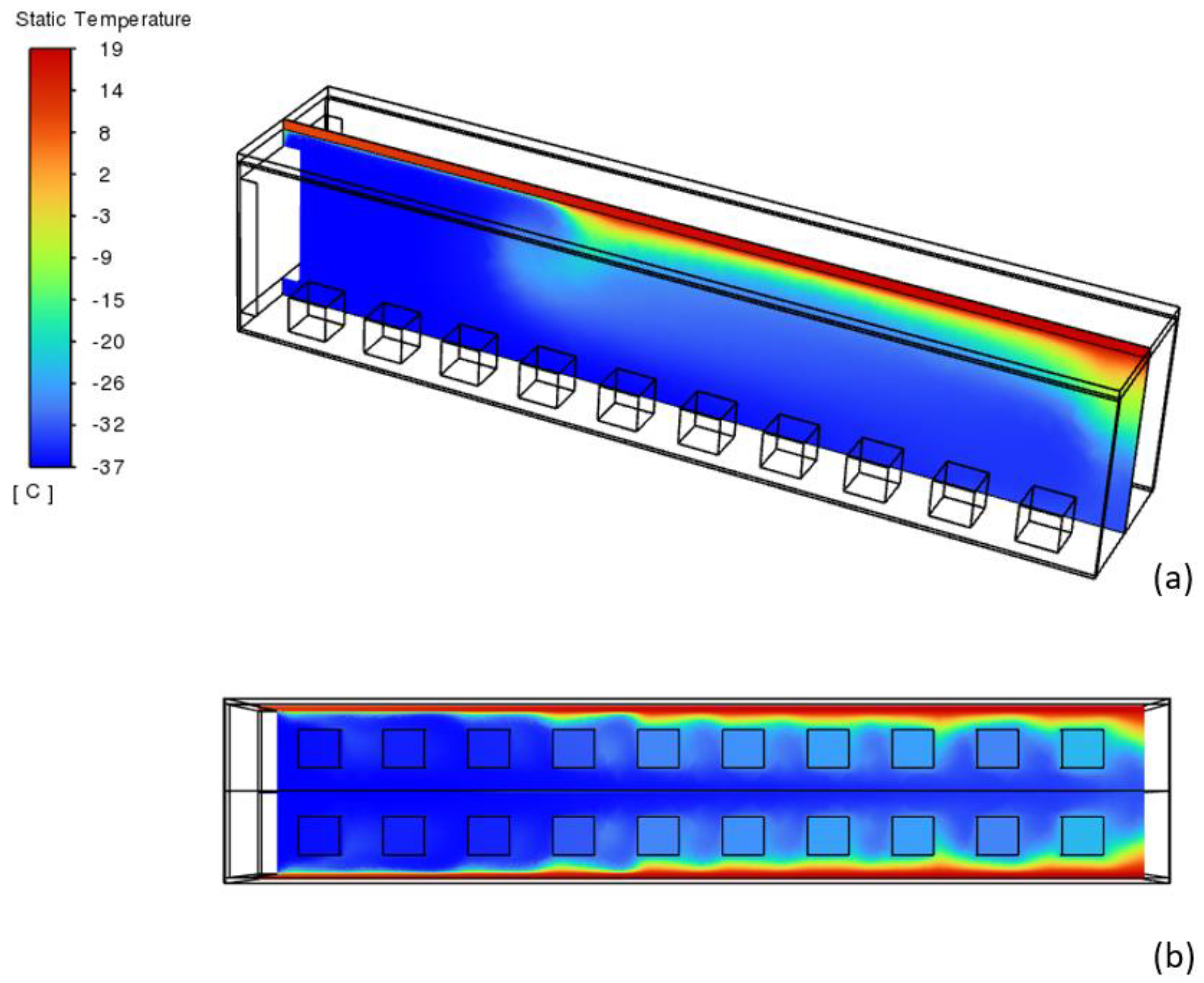
From the above presented validated CFD model, further analysis is performed on the CFD model to reveal comprehensive temperature and velocity vector distribution within the cold container. In
Figure 3, the temperature distribution visualization reveals a significant thermal gradient along the container’s length, with temperatures ranging from −37 °C near the cold air inlet (left side) to approximately −32 °C at the door (right side). The ambient temperature is 20 °C and seems to be well insulated by the high-performance PUR insulation material, thus the thermal stratification shows a clear transition from cold (blue) to warm (red) regions, with the cold zone effectively maintaining low temperatures around the first six boxes but showing reduced cooling efficiency for the boxes closer to the door. The thermal boundary layer development along the container walls and around the boxes is evident, with warmer temperatures accumulating in the upper right region of the container, suggesting potential optimization opportunities for airflow distribution to achieve more uniform cooling throughout the container length.
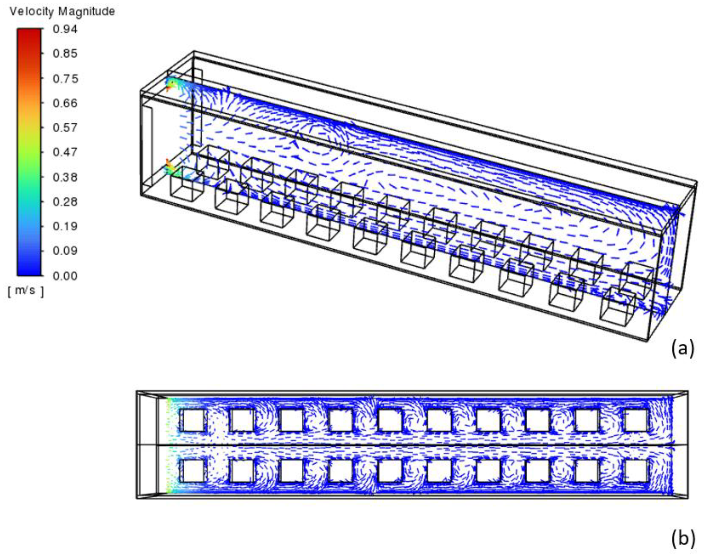
Figure 4 shows that CFD simulation results reveal a complex airflow pattern within the refrigerated container housing 10 uniformly spaced storage boxes. The velocity magnitude distribution, ranging from 0 to 0.94 m/s, demonstrates a predominantly longitudinal flow pattern with significant secondary recirculation zones. This recirculation zone is not observed in [
16], which might be because [
16] modeled a transient flow regime, while the present CFD model used a steady-state simulation. However, air recirculation commonly occurs as the high-velocity flow entrains the surrounding fluid through viscous forces. The entrainment creates pressure gradients within the confined space, forming counter-rotating vortices near the jet entry and secondary patterns downstream, which is observed in similar studies by previous researchers [
18]. From the cross-sectional view in
Figure 4a, the primary air stream exhibits higher velocities along the upper region of the container, while the presence of storage boxes creates distinct wake regions and vertical mixing patterns. The top view in
Figure 4b illustrates the formation of symmetrical vortex structures around each storage box, indicating potential areas of reduced heat transfer efficiency. The return flow configuration, where cold air enters and exits from the left side, generates a gradient in velocity magnitude along the container length, with notably stronger flow characteristics near the inlet region. From
Figure 4, the flow architecture explains the thermal stratification and varying cooling effectiveness across the storage volume that presented in
Figure 4, particularly in the downstream regions where velocity magnitudes decrease substantially due to flow resistance and energy dissipation through the box array.
2.3. Generating Datasets for Machine Learning
As discussed above, while CFD simulation provides detailed spatiotemporal insights into the complex flow patterns within the cold container, the computational intensity and time requirements of these simulations limit their wide applications in operational improvement. By leveraging the high-fidelity CFD data as a training foundation for machine learning models, one can develop rapid prediction capabilities for critical parameters such as local velocity distributions, temperature gradients, and cooling effectiveness. Such machine learning models, once properly trained and validated against CFD results, could have the potential to enable even more effective thermal management. Furthermore, the integration of machine approaches with CFD-generated datasets opens new avenues for identifying nonobvious correlations between process parameters and performance metrics, potentially revealing optimal process control configurations that might not be immediately apparent through traditional parametric CFD studies alone. This hybrid CFD–machine learning methodology represents a promising direction for advancing the efficiency and intelligence of refrigerated container systems while maintaining the physical accuracy inherent in CFD simulations.
To develop a robust machine learning framework for predicting temperature distributions in refrigerated containers, a comprehensive training dataset was generated by systematically varying six key process variables within their operational ranges: air velocity, ambient temperature, cold air temperature, external wall heat transfer coefficient, food thermal conductivity, and PUR insulation thermal conductivity. The output parameters consist of the temperature for each of the ten storage boxes arranged sequentially within the container (see
Figure 1). This parametric approach enables the capture of complex thermal interactions and nonlinear relationships between input variables and resulting temperature distributions, providing a rich dataset for training advanced machine learning algorithms. To minimize bias in generating cases, a Gaussian random generator is used to generate the 205 CFD cases when considering the above input variables. A Gaussian random generator is used in this study to produce case input conditions in the present machine learning study, as it helps avoid bias by naturally representing real-world phenomena, which ensures balanced data representation, and provides useful mathematical properties for weight initialization and data augmentation [
19]. By producing values that follow a Gaussian random distribution, one creates realistic noise patterns that enhance model robustness while maintaining mathematical tractability. The statistical distribution of input parameters, characterized by their respective means and standard deviations, ensures comprehensive coverage of realistic operating conditions while maintaining physical consistency in the generated data, which are detailed in
Table 1. The CFD model cases were run by varying the boundary conditions and material properties in the model setup in the parametric study. For example, different air velocities, ambient temperatures, and external wall heat transfer coefficients are input in the model setup for boundary conditions. The thermal conductivity values for both food and PUR insulation as material properties were varied. In total, 205 cases were run in parallel on a 48-core workstation.
It is important to ensure that the input variables were within reasonable ranges so that the modeled CFD cases represent meaningful physical conditions, especially for material properties. The external wall heat transfer coefficient ranges from low values (e.g., 0.019 W/(m2·K)), representing minimal natural convection, to high values (e.g., 86.4 W/(m2·K)), representing windy weather conditions.
Food thermal conductivity spans from 25.5 W/(m·K) to approximately 100 W/(m·K), as referenced in [
20]. Cold air temperature mostly ranges from very strict frozen conditions, such as storing vaccines at −39.7 °C [
16], to general frozen food conditions at approximately 5 °C [
20].
PUR insulation material made of fiberglass initially has a thermal conductivity of approximately 0.003 W/(m·K) [
21]. However, PUR insulation material degrades when exposed to environmental conditions (e.g., UV radiation from sunlight) and is assumed to degrade to a value only marginally better than particleboard (approximately 0.19 W/(m·K)) in the present study in the worst case [
22].
The same CFD model meshes, which were used in the baseline study presented in
Figure 2,
Figure 3 and
Figure 4, were used for the above machine learning training data generation process. This is because the CFD cases only changed the process and material conditions instead of the structural geometry.
2.4. Machine Learning Model
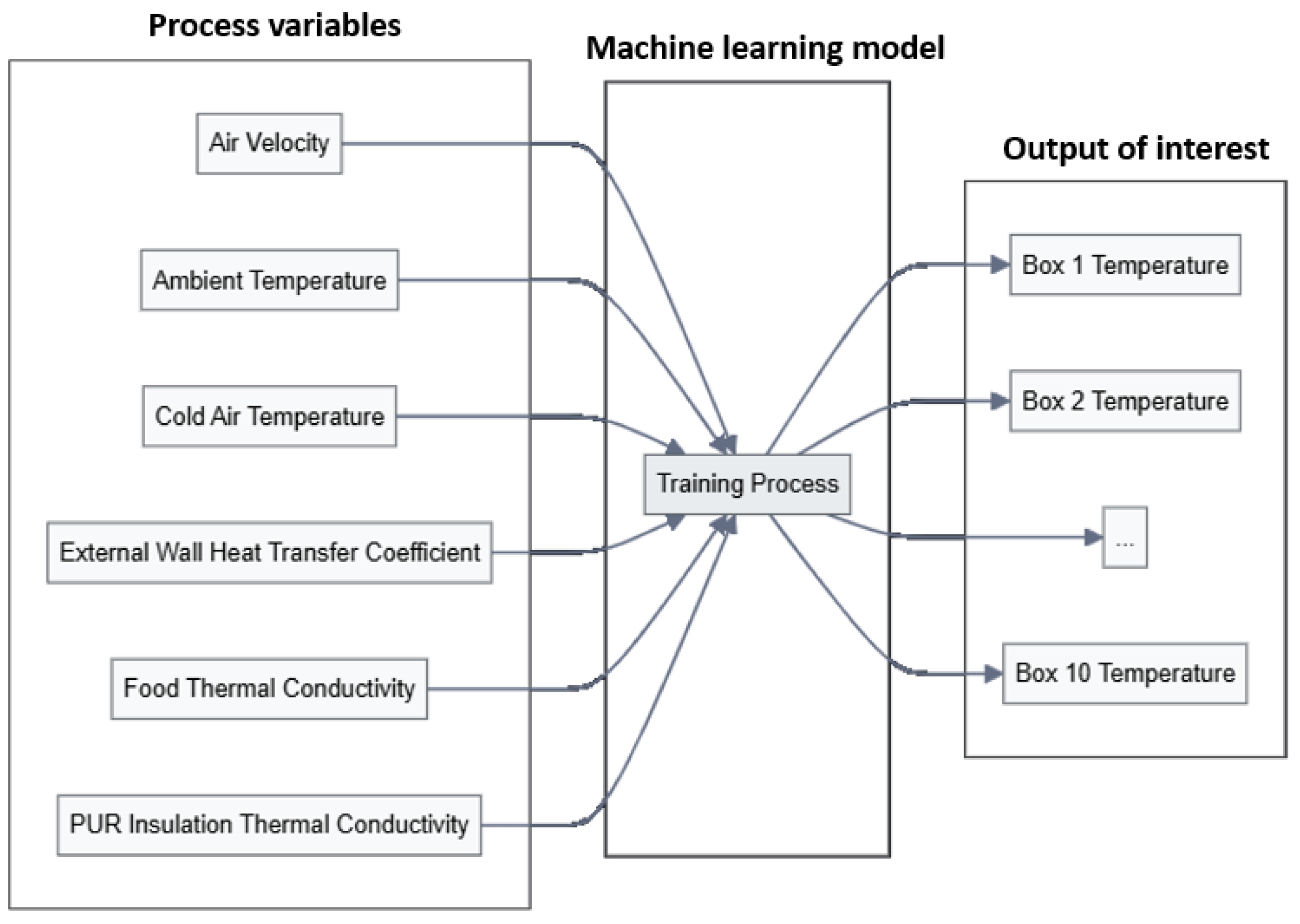
The workflow diagram presented in
Figure 5 illustrates the process of the machine learning model development to predict temperatures in multiple boxes (Box 1 through Box 10) based on six key process variables. The reason why the temperature of each box is output is because proper thermal management in a cold supply chain requires the maximum preservation of frozen food or vaccines, and thus the temperature uniformity of all boxes needs to be monitored and studied. These input variables are fed into a training process within the machine learning model, which then generates temperature predictions for different boxes as outputs of interest for cold container temperature management.
In the present study, two types of machine learning models, Random Forest (RF) and Neural Network (NN), are used. Below shows a brief description of the two models, and more details of the mathematical derivation of these two models can be found in [
23] and [
24], respectively.
2.5. RF Model
A RF model is an ensemble learning method that combines multiple decision trees, each trained on different bootstrap samples of data. The trees independently learn data patterns by optimizing split parameters, and their collective predictions reduce the error propagation that could occur in a single tree, making the model more robust against noise and variations in the dataset [
25].
2.6. NN Model
A NN model is a class of machine learning algorithms designed to replicate the information processing functions of the human brain. The objective of the NN is thermal efficiency. Hidden layers are placed in between the objective and input layers for prediction. In the present model, the activation function for hidden layers uses the Rectified Linear Unit Function (RELU). The hyperparameters (e.g., L2 penalty parameter) are used as defaults within the scikit-learn library, with seven input parameters as the input layer and thermal efficiency as the objective [
13].
NN models have developed rapidly in recent years. A NN can be mathematically considered as a nonlinear regression model
, where
is a nonlinear model function, and w is the vector that contains the parameters in which x is known as the input. The basic units of a NN, known as perceptrons, can be computed as
, where the nonlinear function
is called the activation function. The training of a perceptron model is conducted through the updating of weights as follows [
26]:
where
is the learning rate.
3. Discussion
A RF model uses 200 decision trees with a max depth of 15 and bootstrap sampling, while the NN employs a deep architecture of four hidden layers (256 → 128 → 64 → 32 neurons) with ReLU activation, an Adam optimizer, and an adaptive learning rate. When developing the above machine learning model, 20% of the total generated CFD datasets are used for testing. The accuracy of the developed machine learning models is examined.
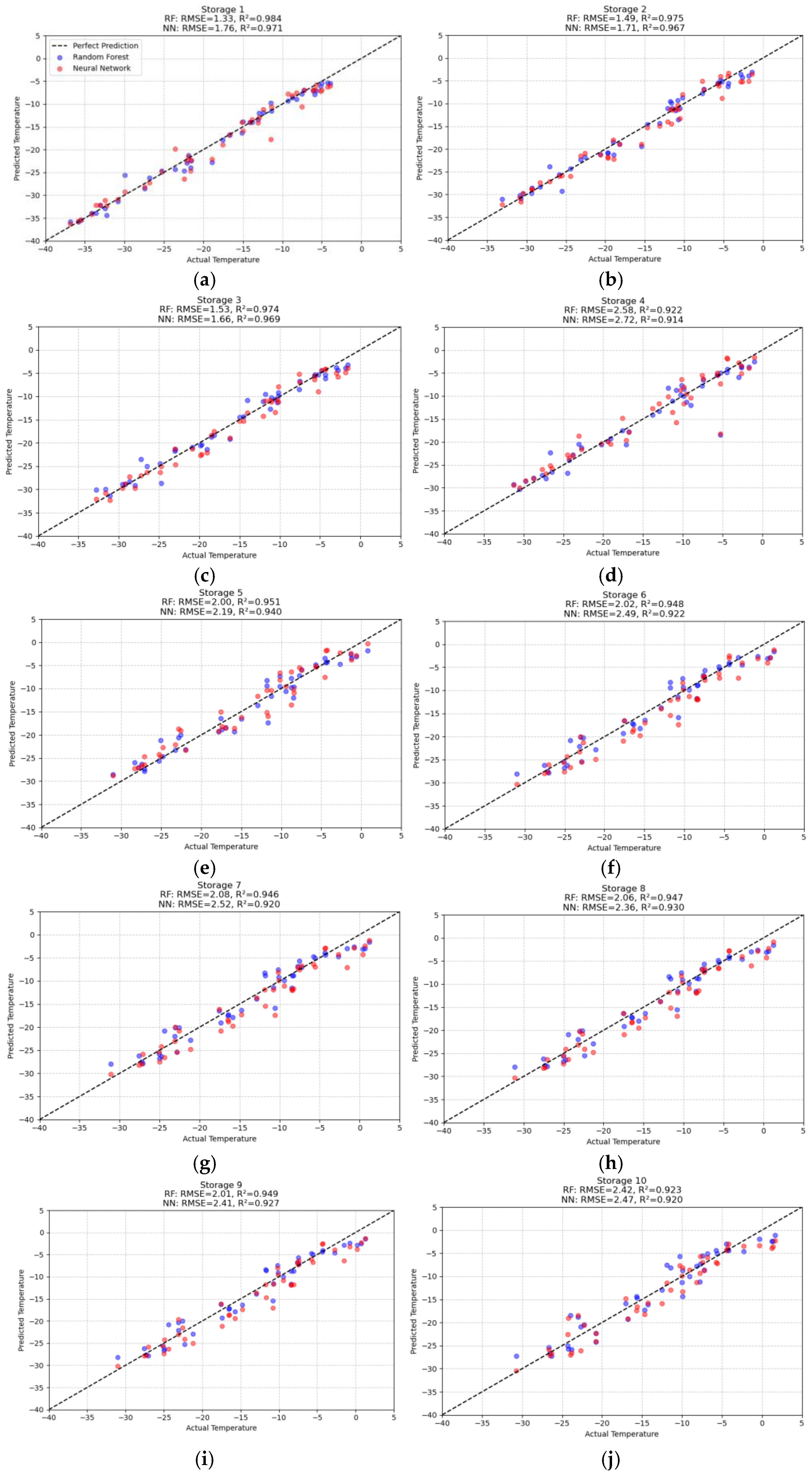
Figure 6 shows the comparative analysis of RF and NN models across ten storage temperature cases. It reveals that RF consistently outperforms the NN across the temperature of ten boxes, particularly evident for storage boxes 1–3, where RF achieves slightly lower RMSE values and higher R
2 values compared to the NN’s. This pattern continues across Storages 4–10, where RF maintains better performance. The performance gap is most pronounced in Storage 6, where RF (RMSE = 2.02 °C, R
2 = 0.948) minorly outperforms the NN (RMSE = 2.49 °C, R
2 = 0.922), demonstrating a 19% advantage in prediction accuracy. These findings indicate that RF models should be the preferred choice for storage temperature prediction under steady-state conditions, offering both better accuracy and more consistent performance across varying storage conditions, while also typically requiring less computational overhead than NN models.
RF’s better performance over the NN in storage temperature prediction may be attributed to three key factors: Firstly, RF’s ensemble approach better captures the relatively stable patterns in steady-state temperature conditions without overcomplicating the relationships. Secondly, a decision tree structure effectively handles nonlinear relationships while remaining robust to outliers and noise, and its simpler architecture may be more appropriate for this specific prediction task, where the underlying temperature relationships are relatively straightforward. This is particularly evident in Storages 1–3, where RF maintains significantly better accuracy, suggesting that more complex NN architectures may be unnecessarily sophisticated for steady-state temperature prediction scenarios.
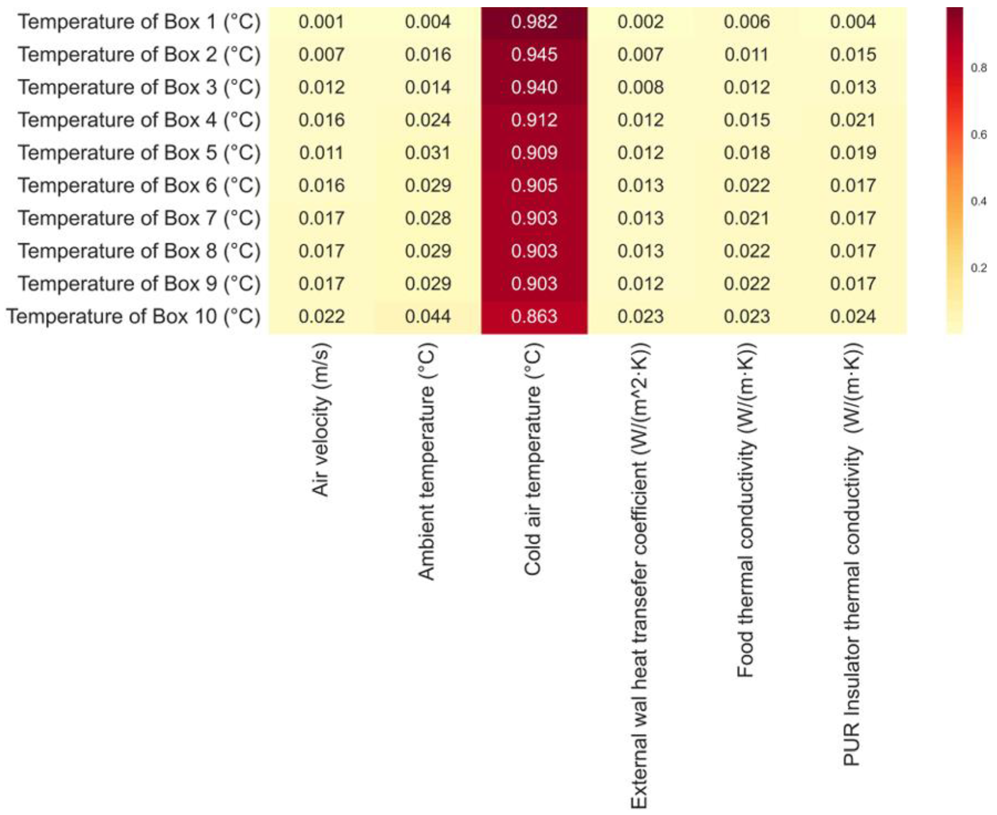
To understand the relative importance of different variable inputs, it is important to display relative feature importance values, showing how much each input variable contributes to determining the temperature of each box.
Figure 7 presents the feature importance heatmap by revealing the key dominant importance of cold air temperature as the primary influential factor across all storage box temperatures, with importance values consistently exceeding 0.86 (86%). This relationship demonstrates a robust hierarchical pattern, where Box 1 exhibits the strongest correlation (0.982) with cold air temperature, followed by a gradual decrease in importance through Box 10 (0.863). The remaining environmental parameters, including air velocity, ambient temperature, external wall heat transfer coefficient, food thermal conductivity, and PUR insulator thermal conductivity, demonstrate notably lower importance values (generally below 0.044), suggesting their relatively minimal impact on storage temperature variations. This shows the importance values indicate that the thermal management system’s performance is predominantly governed by cold air temperature regulation, while other thermal and fluid dynamic parameters play subsidiary roles in maintaining desired storage conditions.
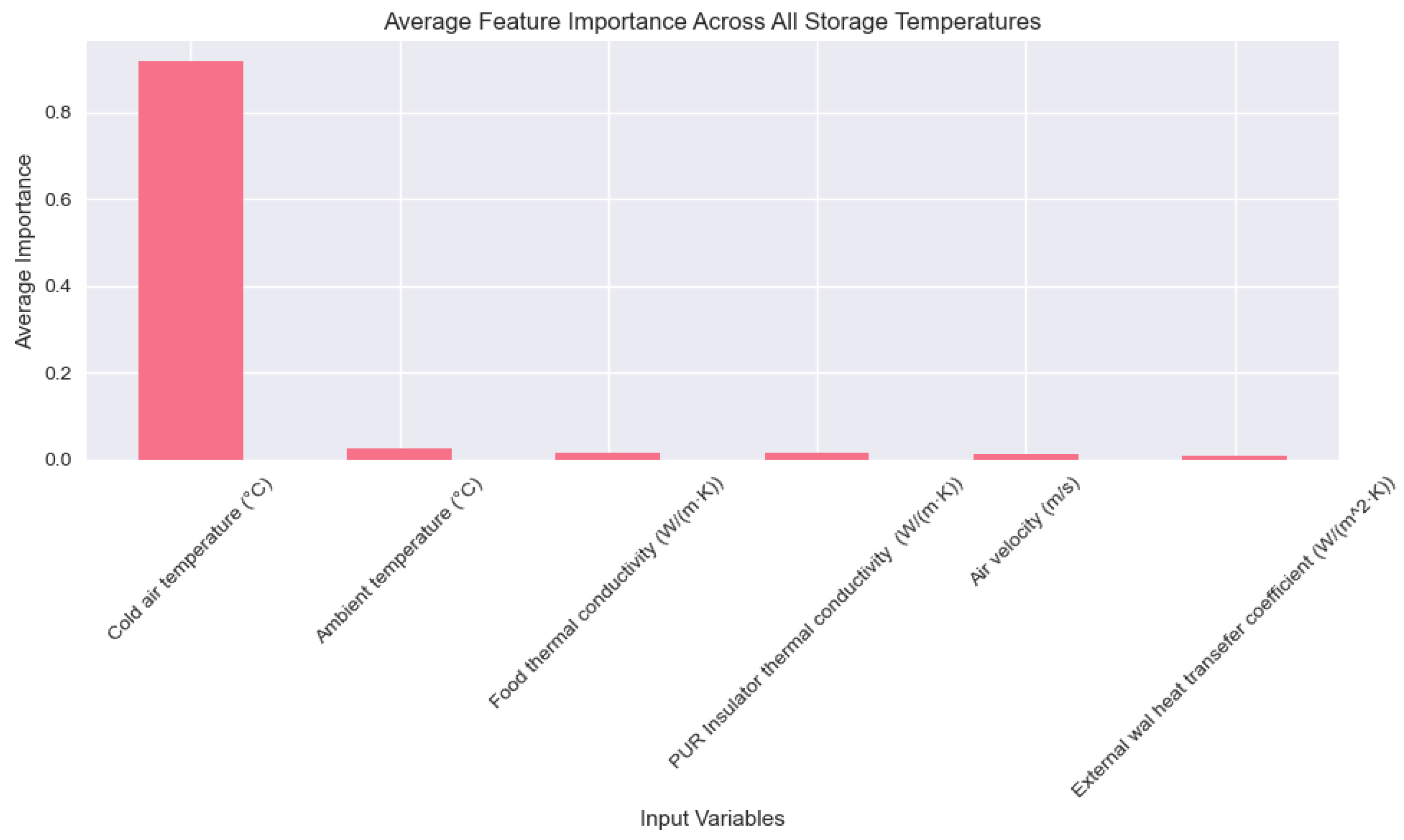
Figure 8 confirms observations from
Figure 7, establishing cold air temperature as the dominant factor in storage temperature control (importance: 0.917), which far exceeds ambient temperature, PUR insulation, food thermal conductivity, air velocity, and wall heat transfer. This demonstrates the system’s primary dependence on cold air temperature regulation, suggesting optimization efforts should prioritize precise control of this parameter while treating others as secondary factors in thermal management.
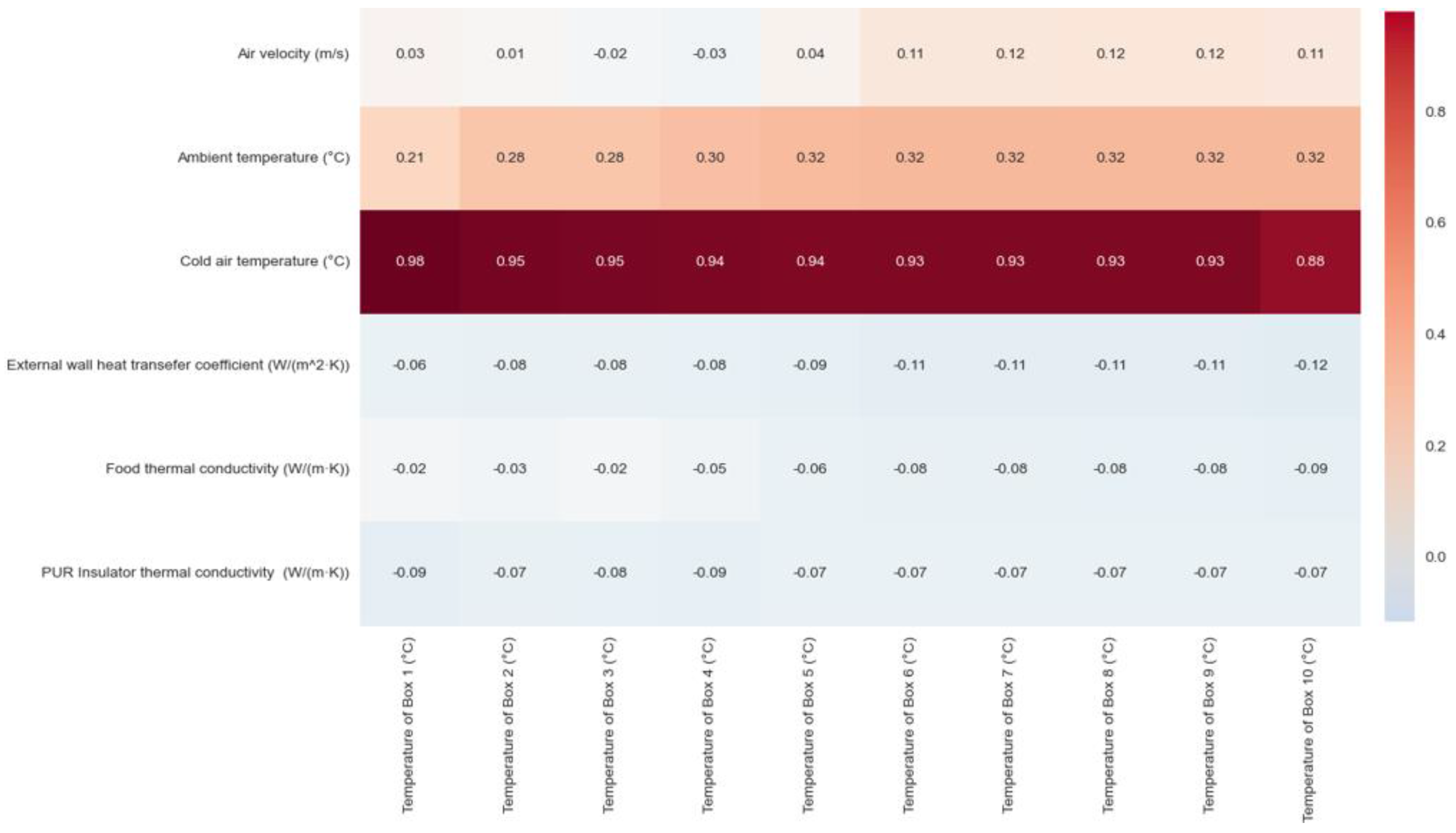
Figure 9 reveals cold air temperature has the strongest positive correlation with storage temperature, decreasing from Box 1 to 10. Ambient temperature shows a moderate positive correlation, increasing across the boxes. Thermal conductivity and wall heat transfer show weak negative correlations, while air velocity effects appear distance-dependent. These findings confirm cold air temperature as the primary factor for maintaining desired storage conditions.
Referring to both
Figure 7 and
Figure 9 provides valuable understanding because feature importance reveals causal influence within a model (which factors drive predictions), while correlation simply shows statistical relationships without implying causation, and altogether these highlight that cold air temperature is both highly important (0.86–0.98) and strongly correlated (0.88–0.98) with box temperature. Thus, this provides complementary insights for understanding the thermal dynamics of the cold container system.
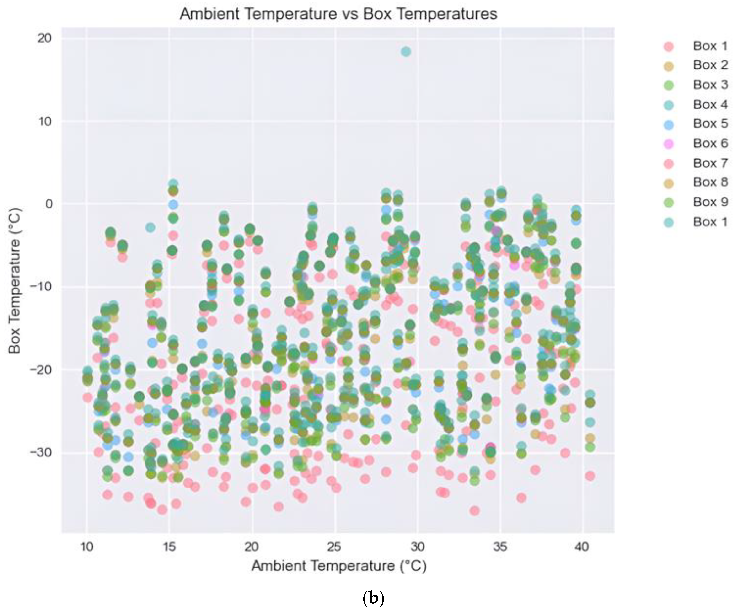
Based on the above analysis, it shows that cold air temperature and ambient temperature are the two most important variables that determine the thermal performance of storage boxes inside cold containers. To further understand the role of these two input variables,
Figure 10 presents a dual scatter plot analysis to reveal distinctly different relationships between storage box temperatures and the two input variables. The left panel demonstrates a strong positive linear correlation between cold air temperature (−40 °C to −5 °C) and box temperatures, with correlation coefficients consistently above 0.88 across all boxes. Box 1 (pink markers) consistently maintains the lowest temperatures, with subsequent boxes showing incrementally higher temperatures, indicating a systematic thermal gradient across the storage system. In contrast, the right panel illustrates a notably weaker and more dispersed relationship between ambient temperature (10 °C to 40 °C) and box temperatures, characterized by substantial scatter and limited correlation (correlation coefficients ranging from 0.21 to 0.32). This comparative visualization effectively highlights the dominant influence of cold air temperature on the storage system’s thermal behavior, while ambient temperature exhibits minimal impact on internal box temperatures, likely due to effective insulation. This shows that PUR insulation material is very effective at providing sufficient thermal insulation between the cold air and the ambient environment in general. The outliers in
Figure 10 may be due to recirculation patterns creating isolated thermal environments that differ significantly from the general trend. These recirculation zones resulting from pressure differentials cause warmer air to circulate back into certain box locations despite the overall cold air temperature setting.
Interpretability is an important aspect of machine learning models. One of the most used methods for interpretability evaluation is SHapley Additive exPlanation (SHAP). The SHAP analysis reveals distinct patterns of feature importance and their impacts on machine learning model predictions for outputs of interest (e.g., temperature of boxes in the cold container in the present study). It provides a mathematical framework for interpreting machine learning model predictions by assigning each feature an importance value based on game theory principles [
25]. It addresses the “black box” nature of machine learning models by quantifying both individual and interactive effects of input variables on model outputs, enabling model validation behavior against physical principles and deriving actionable insights for system optimization.
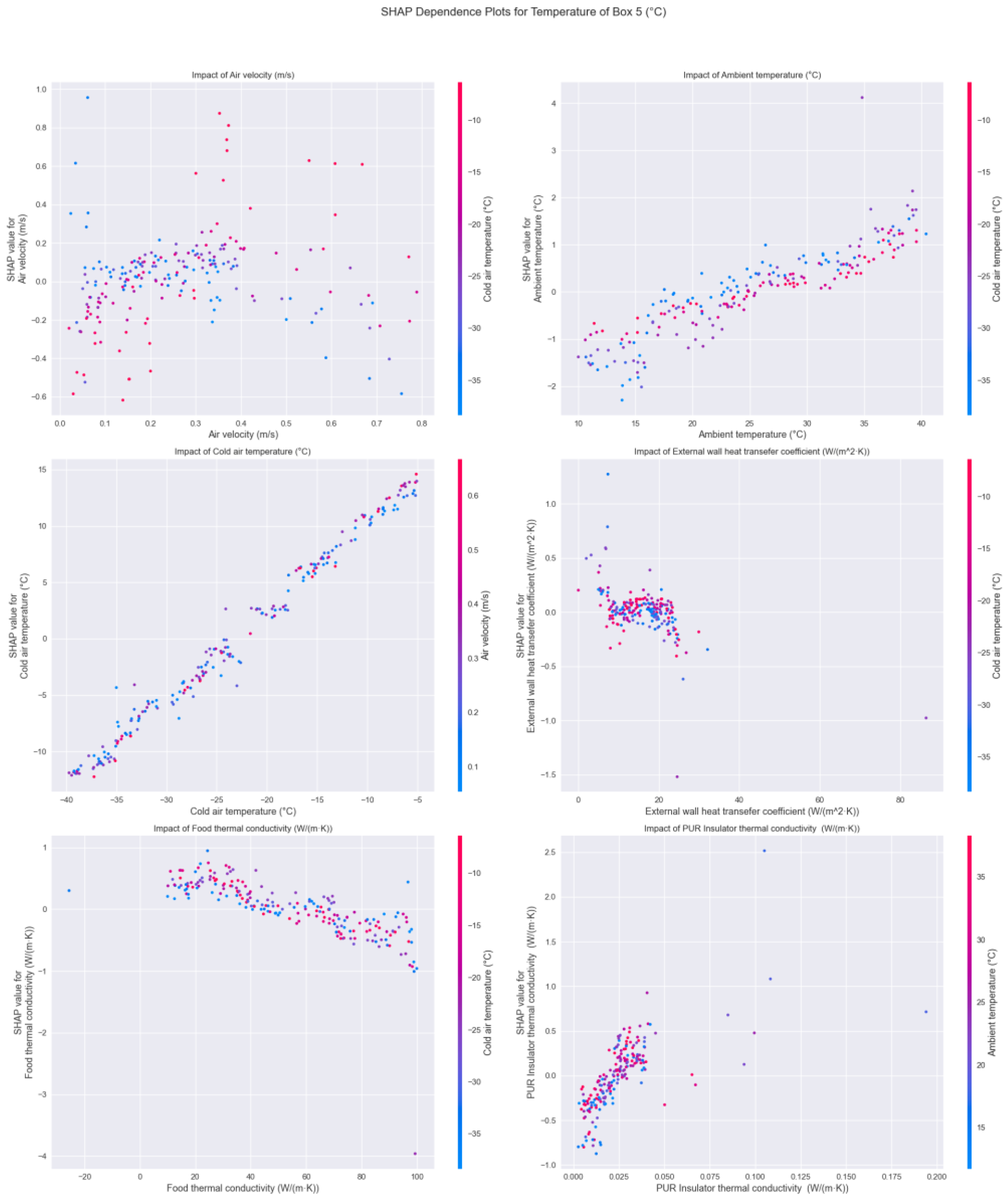
Storage box 5 is chosen for SHAP analysis, and the results are presented in
Figure 11. From
Figure 11, SHAP dependence analysis of Box 5’s temperature control system reveals complex thermal interactions across six key parameters. Cold air temperature (e.g., ranging from −40 to −5 °C for frozen food) demonstrates the strongest linear correlation, establishing itself as the primary control variable, while ambient temperature (e.g., 10–40 °C, which covers typical environment temperatures) shows a robust positive linear relationship, indicating its significant external influence. Air velocity exhibits optimal cooling effectiveness between 0.2 and 0.4 m/s, with diminishing returns at higher velocities, suggesting a critical operational range for system efficiency. The external wall heat transfer coefficient shows clustered behavior below 20 W/(m
2·K), indicating a potential optimization threshold. Food thermal conductivity (e.g., <100 W/(m·K)) displays a negative correlation, with considerable scatter, highlighting the importance of product-specific considerations. Thermal conductivity of PUR insulation material (e.g., <0.200 W/(m·K)) demonstrates a weak positive correlation with high variability, suggesting its role as a secondary factor in temperature control.
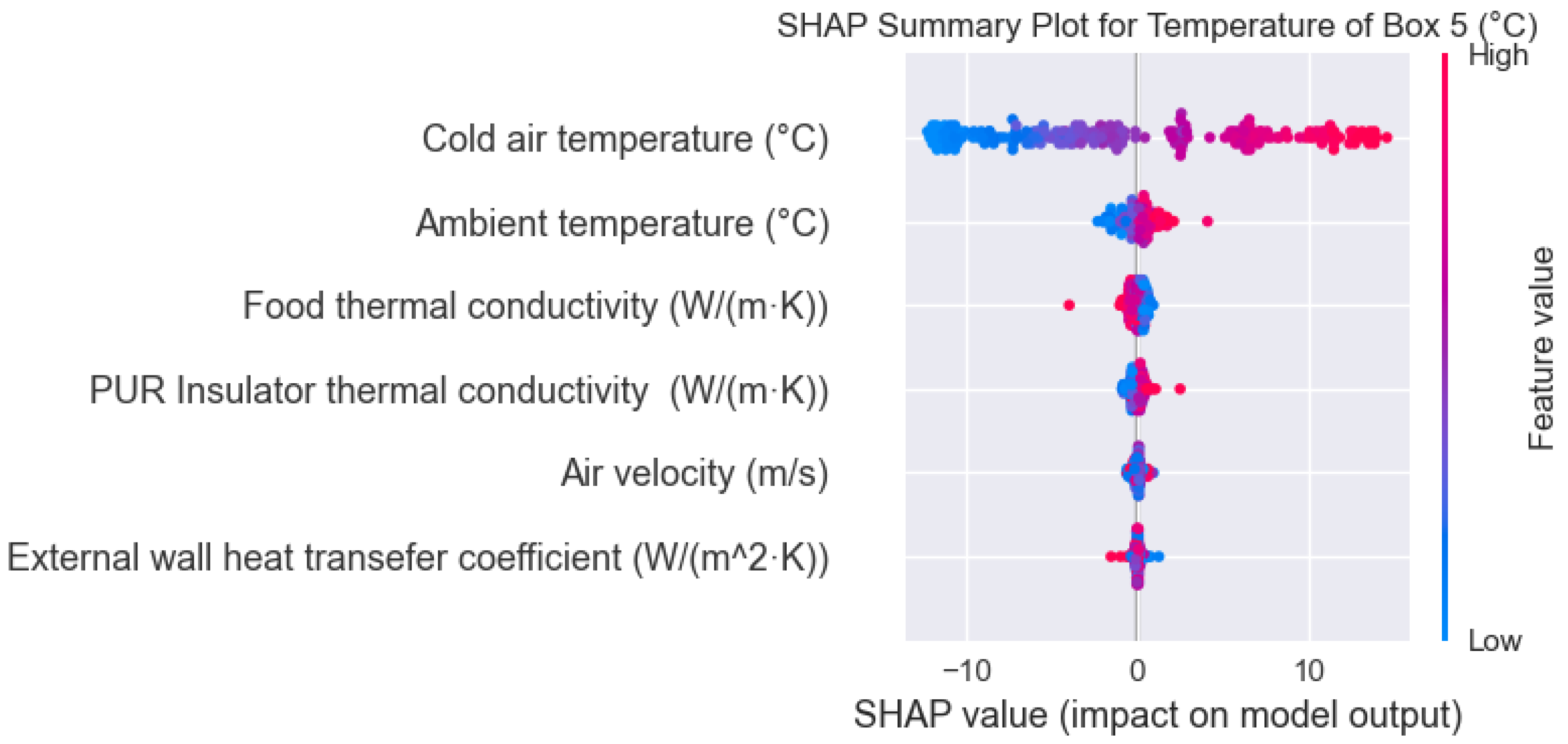
In
Figure 12, the SHAP summary plot analysis of Box 5’s temperature control system reveals a distinct hierarchical influence of thermal and physical parameters on system performance. Cold air temperature emerges as the dominant control variable, exhibiting the most extensive SHAP value distribution (−10 to +10) with a pronounced bimodal pattern, indicating its critical role in system control. Ambient temperature demonstrates a secondary but significant influence, with moderate SHAP values (−5 to +5) and clear temperature-dependent effects, highlighting the importance of environmental conditions. Food thermal conductivity, PUR insulator conductivity, air velocity, and external wall heat transfer coefficient display progressively diminishing impacts, with their SHAP values clustered tightly around zero, suggesting their roles as less important factors. These findings indicate that system optimization should prioritize precise cold air temperature control mechanisms and robust ambient temperature compensation while maintaining cost-effective management of secondary parameters. This hierarchical understanding enables targeted design improvements and operational strategies, potentially leading to enhanced system efficiency through focused control system development and resource allocation.


