Shape Optimization of the Triangular Vortex Flowmeter Based on the LBM Method

Abstract

In this paper, the D3Q19 multiple-relaxation-time (MRT) lattice Boltzmann method (LBM) for large eddy simulation (LES) was employed to optimize the shape of the vortex generator in a triangular vortex flowmeter. The optimization process focused on the vortex shedding frequency, lift force per unit area, and symmetry of the vortex street. The optimal shape of the vortex generator was determined to feature a 180° incoming flow surface, a concave arc side with a curvature radius of 25 mm, and a fillet radius of 4 mm at the end. Numerical simulations revealed that the optimized vortex generator achieves a 2.72~13.8% increase in vortex shedding frequency and a 17.2~53.9% reduction in pressure drop and can adapt to the flow conditions of productivity fluctuations (6.498 × 10⁵ ≤ Re ≤ 22.597 × 10⁵) in the gas well production. The results demonstrated significant advantages, including low pressure loss, minimal secondary vortex generation, high vortex shedding frequency, and substantial lift force. These findings underscore the robustness and efficiency of the LBM-LES method in simulating complex flow dynamics and optimizing vortex generator designs.

1. Introduction

The vortex flowmeter is widely used in flow measurement of liquid, gas, and steam. To obtain accurate flow measurement results, a vortex generator with excellent performance is necessary to generate strong and stable vortexes [1]. In recent years, many researchers have studied the flow measurement characteristics of different vortex generators through numerical simulation and experimental methods. It is generally believed that the lower limit of Re for vortex flowmeter application is 20,000, the applicable flow rate in gas phase fluid is 6~80 m/s, and that, in liquid phase, fluid is 0.3~9 m/s [2]. In practical applications, the vortex signals generated by the generators of different shapes and sizes vary greatly in terms of intensity and stability [3,4]. Especially at low flow rate, the vortex intensity generated by most vortex generators will weaken. The vortex generator is usually made of easily machined monomers such as cylinders, trapezoids, and triangles [5,6]. Later, it gradually developed into the multi-body generator with slits perpendicular to the flow direction, but the slits were difficult to produce and easy to be blocked by impurities, so they were not widely used in the industry [7,8]. The trapezoid generator has obvious secondary vortexes [9]. The interference of secondary vortexes during signal processing increases the detection difficulty of vortex frequency. The cylindrical generator has the problems of low vortex intensity and low vortex shedding frequency [10]. 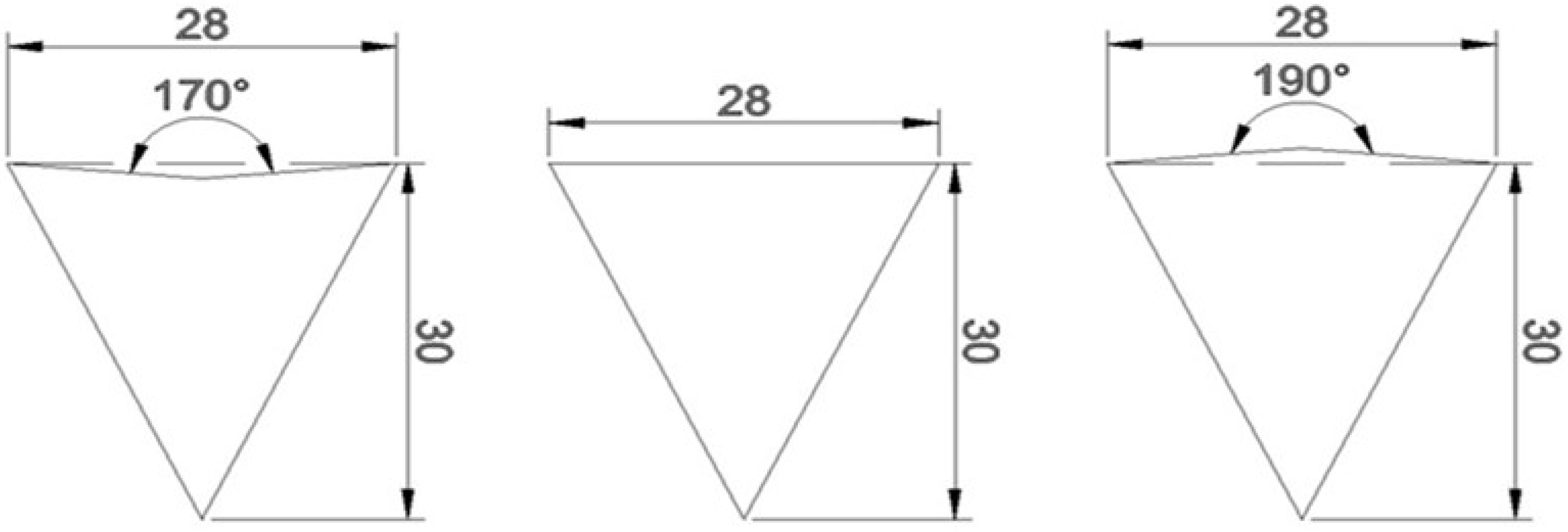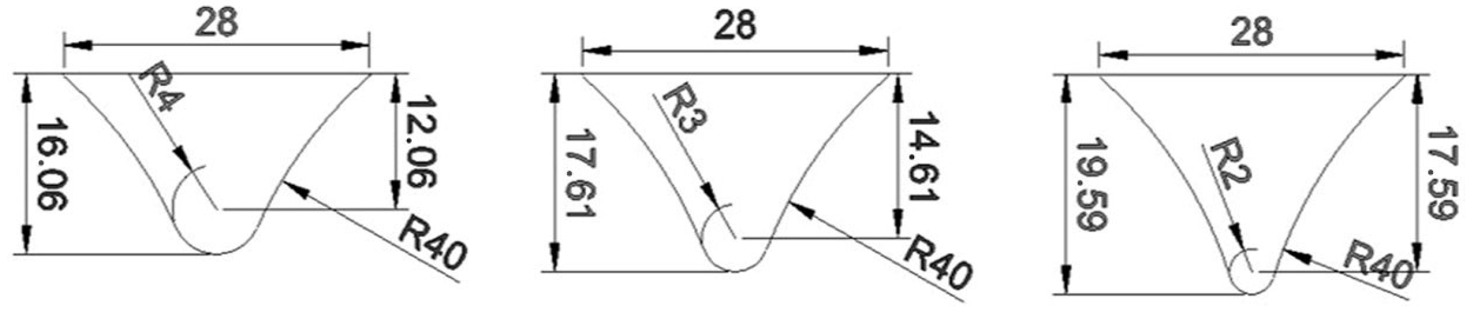Therefore, the triangular vortex flowmeter is widely used in the industry [11]. In this paper, taking Well A2 of Lingshui Gas Field in the South China Sea as an example, we optimized its shape based on the triangular vortex generator so that the optimized vortex generator can be applied to the low productivity stage of the gas well. The new vortex generator is mainly optimized from the incoming flow surface, the side, and the end. There is no sharp shape mutation inflection point at the end of the new generator, and the side is a concave arc shape, which can reduce the generation of secondary vortexes and the interference of noise signals. The concave arc shape of the side is conducive to the reverse expansion of the vortex, reducing the impact of the main flow on the vortex and increasing the vortex intensity [12].

The shedding frequency of the vortex generator can be calculated by two methods [13]. It can be calculated by the Strouhal number (St), which is a dimensionless parameter to characterize the linear relationship between the measured vortex frequency and the flow rate. The expression is shown below:

$$St={\displaystyle \frac{fd}{v}}$$

(1)

In the above equation, $f$ is vortex shedding frequency, Hz; $d$ is the width of bluff body, m; and $\nu$ is the mean velocity determining the volumetric flowrate, m/s.

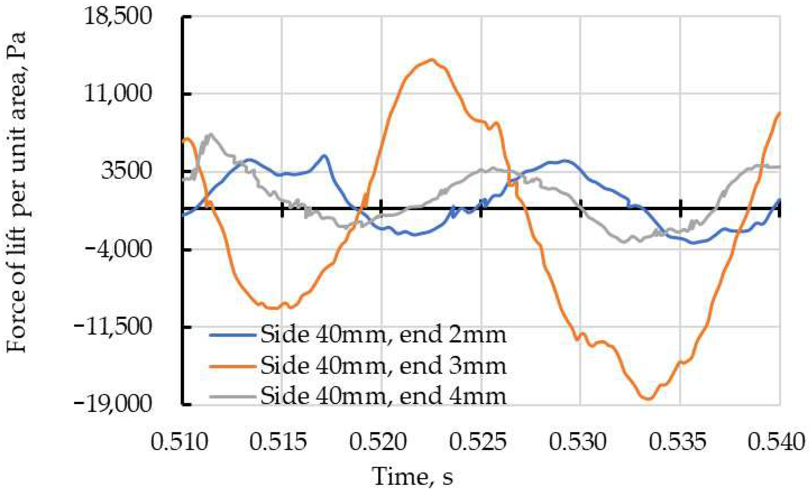
The shedding frequency can also be obtained through fast Fourier transform (FFT) by actually measuring the stable lift force curve generated by the vortex generator [14]. In this paper, the LBM method was used to simulate the vortex flowmeter used in the gas field. Through the statistics of the surface lift force of the vortex generator, the vortex shedding frequency of the vortex generator was obtained using the FFT method, then the vortex intensity and the symmetry of the vortex array were clarified.

At present, the numerical simulation study on the flow around the cylinder of the vortex flowmeter mainly focuses on the 2D plane simulation, while there are relatively few numerical studies under 3D conditions, because in the 3D case, the flow around the cylinder is affected by the wall boundary layer and turbulent disturbance in multiple directions, the vortex intensity is small, and the turbulence phenomenon is not obvious [15]. On the 2D plane, the flow around the cylinder is obvious, the frequency and lift force of the vortex are stable, and it is easy to distinguish the advantages of various vortex generators [16]. Currently, the flow around the cylinder is mainly analysed through finite difference method (FDM), finite volume method (FVM), finite element method (FEM), lattice Boltzmann method (LBM), and other numerical methods. Geller basically calculated the laminar flow using the LBM and FEM methods and demonstrated the effectiveness of various algorithms [17]. Pietro applied large eddy simulation (LES) to calculate the flow around the cylinder at high Reynolds number and proved that the result of LES was more accurate than that of Reynolds-averaged Navier–Stokes (RANS) [18]. Al-Jahmany tested the computational performance of the LBM and FVM methods by simulating laminar flow in pipelines [19]. The results showed that both methods yield consistent flow rate and stress values, but LBM demonstrates significantly higher computational efficiency. Building on this, Haussmann conducted a 3D numerical simulation of flow around a cylinder using both methods and compared their computational accuracy [20]. The results revealed that the drag coefficient calculated by the LBM method is closer to the experimental value compared to FVM.

For the turbulence problem at high Reynolds number, the sub-grid-scale stress model (SGS) for large eddy simulation can be introduced into the LBM method. Xia et al. introduced the k-ω and Spalart–Allmaras turbulence model (S-A) into the single relaxation time lattice Boltzmann method (SRT-LBM) separately and numerically simulated the backward-facing step flow at high Reynolds number in combination with the unstructured grid technology. The result showed that for the backward-facing step flow, the calculation accuracy of the k-ω turbulence model was higher than that of the S-A turbulence model [21]. Bartlett et al. introduced the k-ε turbulence model into SRT and numerically simulated the flow around the cylinder at high Reynolds number [22]. Eggels et al. combined the turbulence stress tensor with the equilibrium distribution function in LBM and gave the average physical quantity of flow field and turbulence intensity of a large eddy simulation, etc., which are in good agreement with the experimental data [23]. The result showed that the sub-grid model of LBM has the potential to simulate complex flow conditions or turbulence at high Reynolds number. Wang et al. introduced the LES model on LBM and calculated the characteristics of the flow around the two-dimensional hydrofoil with a certain angle of attack when the Reynolds number was 5 × 10⁵ and 6.6 × 10⁵, which was highly consistent with the experimental results [24]. LBM can be combined with the LES model (LBM-LES) to overcome the complexity of turbulence at high Reynolds number. In this paper, we applied the LBM-LES method with good parallelism and simple boundary condition processing to obtain the flow field characteristics of turbulence at high Reynolds number under reasonable computing resources.

2. Numerical Method

LBM is a CFD method not based on the continuous medium hypothesis. In this method, the fluid and its time and space of existence are discretized completely. In a time step, discrete fluid particles can only move from the current grid point to adjacent grid points along the grid point connection direction. This process is called migration. When particles from different directions meet on a grid point, they will collide [25]. The collision rules satisfy the local mass conservation, momentum conservation, and energy conservation of the system before and after the collision. In this paper, we employed the open-source program framework OpenLB for numerical simulation of the vortex generator based on the D3Q19 multiple-relaxation-time lattice Boltzmann method for large eddy simulation (MRT-LBM-LES).

2.1. Multiple-Relaxation-Time Lattice Boltzmann Method

In LBM, the velocity space distribution function is transformed into the moment space with the transformation matrix M. The collision process of the distribution function is not completed in the velocity space but in the moment space by linear transformation. This collision form can provide the relaxation process of physical quantities at different time scales [26,27]. Thus, the relaxation process of all physical quantities in the LBM model towards their equilibrium state on the same time scale is avoided. The evolution equation of D3Q19 square grid SRT-LBM can be expressed as below:

$$f_{\alpha }\left(x_i+e_{\alpha }{\delta }_t,t+{\delta }_t\right)-f_{\alpha }\left(x_i,t\right)=-{\displaystyle \frac{1}{\tau }}\left(f_{\alpha }\left(x_i,t\right)-f_{\alpha }^{eq}\left(x_i,t\right)\right)$$

(2)

where $f_{\alpha }$ is the particle velocity distribution function; $\tau$ is the collision relaxation factor, $\tau ={\tau }_0/{\delta }_t$; ${\tau }_0$ is the collision relaxation time; $e_{\alpha }$ is the microscopic velocity set; ${\delta }_t$ is the time step size; and $f_{\alpha }^{eq}$ is the equilibrium distribution function of 19 particles based on Maxwell distribution expansion, and its expression is shown below:

$$f_{\alpha }^{eq}\left(x_i,t\right)=\left\{\begin{array}{cc}{\rho }_0-\left(1-{\omega }_0\right){\displaystyle \frac{p}{c_s^2}}+{\omega }_0& for \alpha =0\\ {\omega }_{\alpha }\rho \left[1+e_{\alpha }{\displaystyle \frac{c_{\alpha i}{u}_i}{c^2}}+{\displaystyle \frac{9}{2}}{\displaystyle \frac{{\left(c_{\alpha i}{u}_i\right)}^2}{c^4}}-{\displaystyle \frac{3}{2}}{\displaystyle \frac{u_i{u}_i}{c^2}}\right]& for \alpha =1\dots 18\end{array}\right.$$

(3)

where $c$ is the discrete particle velocity, generally, $c={\delta }_x/{\delta }_t=1$; $\omega$ is the weight value, ${\omega }_0$ = 1/3, ${\omega }_{1-6}$ = 1/18, ${\omega }_{7-18}$ = 1/36; $c_s$ is the speed of sound, $c_s={\displaystyle \raisebox{1ex}{$c$}\!\left/ \!\raisebox{-1ex}{$\sqrt{3}$}\right.}$; $a$ is denotes the possible direction of the particle velocity; $u_i$ is the macroscopic velocity; and $e_{\alpha }$ is expressed in the D3Q19 grid as follows:

$$e_{\alpha }=\left\{\begin{array}{cc}(0,0,0)& for \alpha =0\\ (\pm 1,0,0)c,(0,\pm 1,0)c,(0,0,\pm 1)c,& for \alpha =1\dots 6\\ (\pm 1,\pm 1,0)c,(\pm \mathrm{1,0},\pm 1)c,(0,\pm 1,\pm 1)c,& for \alpha =7\dots 18\end{array}\right.$$

(4)

In order to obtain the macroscopic equation, the proper weight value should be selected so that $f_{\alpha }^{eq}$ satisfies the constraints of mass conservation, momentum conservation, and isotropy [28]. That is, it should satisfy the following:

$${\rho }_0={\sum }_{\alpha =0}^{18}{f}_{\alpha }^{eq}\left(x_i,t\right)={\sum }_{\alpha =0}^{18}{f}_{\alpha }\left(x_i,t\right),$$

(5)

and

$${\rho }_0{u}_i={\sum }_{\alpha =0}^{18}{f}_{\alpha }^{eq}\left(x_i,t\right)e_{i\alpha }={\sum }_{\alpha =0}^{18}{f}_{\alpha }\left(x_i,t\right)e_{i\alpha },$$

(6)

The evolution equation of D3Q19 square grid MRT-LBM can be expressed as follows:

$$f_{\alpha }\left(x_i+e_{\alpha }{\delta }_t,t+{\delta }_t\right)-f_{\alpha }\left(x_i,t\right)=-{\mathit{S}}_{\alpha \beta }\left(f_{\beta }\left(x_i,t\right)-f_{\beta }^{eq}\left(x_i,t\right)\right)$$

(7)

where ${\mathit{S}}_{\alpha \beta }$ is the diagonalizable collision matrix, and the two eigenvalues are between 0 and 2. We suppose there is an invertible matrix $\mathit{M}$ and a diagonal matrix $\mathit{S}$, which satisfy the following transformation relation:

$${\mathit{S}}_{\mathit{\alpha }\mathit{\beta }}={\mathit{M}}^{-1}\mathit{S}\mathit{M}$$

(8)

Then, the transformation between the velocity space distribution function and the moment space vector can be realized by using the transformation matrix $\mathit{M}$ of the collision matrix $\mathit{S}$, and the Equation (7) can be rewritten as follows:

$$f_{\alpha }\left(x_i+e_{\alpha }{\delta }_t,t+{\delta }_t\right)-f_{\alpha }\left(x_i,t\right)=-{\mathit{M}}^{-1}\mathit{S}\mathit{M}\left[f_{\alpha }(x_i,t)-f_{\alpha }^{eq}(x_i,t)\right]$$

(9)

$$m=\mathit{M}{f}_{\alpha },f_{\alpha }={\mathit{M}}^{-1}m$$

(10)

$$f_{\alpha }\left(x_i+e_{\alpha }{\delta }_t,t+{\delta }_t\right)-f_{\alpha }\left(x_i,t\right)=-{\mathit{M}}^{-1}\mathit{S}\left[m(x_i,t)-m^{eq}(x_i,t)\right]$$

(11)

where $m$ is moment-space modal vector and is a polynomial function of the discrete velocity vector $e_{\alpha }$.

$$m_{\alpha }=\left(\rho ,e,\delta ,j_x,q_x,j_y,q_y,j_z,q_z,3p_{xx},p_{ww},p_{xy},p_{yz},p_{zx},m_{xyz}\right)$$

(12)

The parameters in the equation are defined as follows:

$$e^{eq}=-\rho +{\displaystyle \frac{1}{{\rho }_0}}{j}_i{j}_i$$

(13)

$${ϵ}^{eq}=-\rho$$

(14)

$$q_x^{eq}=-{\displaystyle \frac{7}{3}}{j}_x,q_y^{eq}=-{\displaystyle \frac{7}{3}}{j}_y,q_z^{eq}=-{\displaystyle \frac{7}{3}}{j}_z$$

(15)

$$p_{xy}^{eq}={\displaystyle \frac{1}{{\rho }_0}}{j}_x{j}_y,p_{yz}^{eq}={\displaystyle \frac{1}{{\rho }_0}}{j}_y{j}_z,p_{xz}^{eq}={\displaystyle \frac{1}{{\rho }_0}}{j}_x{j}_z$$

(16)

$$m_{xyz}^{eq}=0$$

(17)

where $j_i$ is the momentum component; $q_i^{eq}$ is the energy flux; $p_{xy}^{eq}$, $p_{yz}^{eq}$, and $p_{xz}^{eq}$ are related to the diagonal and non-diagonal components of the stress tensor; and, according to the law of conservation, ${\rho }_0$ and $j_i$ are 0.

In the D3Q19 model, the physical viscosity only applies to the moment vectors of $m_9,m_{11},m_{13},m_{14}$, and $m_{15}$ [29]. Therefore, the relaxation time matrix is as follows:

$$\mathit{S}=diag(\mathrm{0,1.19,1.4,0},\mathrm{1.2,0},\mathrm{1.2,0},1.2,\nu ,1.4,\nu ,1.4,\nu ,\nu ,\nu ,\mathrm{1.98,1.98,1.98})$$

(18)

The transformation matrix M from the velocity space to the momentum space is as follows:

$$M=\left|\begin{array}{cccc}1& 1& 1& 1\\ -30& -11& -11& -11\\ 12& -4& -4& -4\\ 0& -1& 0& 0\\ 0& 4& 0& 0\\ 0& 0& -1& 0\\ 0& 0& 4& 0\\ 0& 0& 0& -1\\ 0& 0& 0& 4\\ 0& 2& -1& -1\\ 0& -4& 2& 2\\ 0& 0& 1& -1\\ 0& 0& -2& 2\\ 0& 0& 0& 0\\ 0& 0& 0& 0\\ 0& 0& 0& 0\\ 0& 0& 0& 0\\ 0& 0& 0& 0\\ 0& 0& 0& 0\end{array}\begin{array}{ccccccc}1& 1& 1& 1& 1& 1& 1\\ 8& 8& 8& 8& 8& 8& -11\\ 1& 1& 1& 1& 1& 1& -4\\ -1& -1& -1& -1& 0& 0& 1\\ -1& -1& -1& -1& 0& 0& -4\\ -1& 1& 0& 0& -1& -1& 0\\ -1& 1& 0& 0& -1& -1& 0\\ 0& 0& -1& 1& -1& 1& 0\\ 0& 0& -1& 1& -1& 1& 0\\ 1& 1& 1& 1& -2& -2& 2\\ 1& 1& 1& 1& -2& -2& -4\\ 1& 1& -1& -1& 0& 0& 0\\ 1& 1& -1& -1& 0& 0& 0\\ 1& -1& 0& 0& 0& 0& 0\\ 0& 0& 0& 0& 1& -1& 0\\ 0& 0& 1& -1& 0& 0& 0\\ -1& -1& 1& 1& 0& 0& 0\\ 1& -1& 0& 0& -1& -1& 0\\ 0& 0& -1& 1& 1& -1& 0\end{array}\begin{array}{ccc}1& 1& 1\\ -11& -11& 8\\ -4& -4& 1\\ 0& 0& 1\\ 0& 0& 1\\ 1& 0& 1\\ -4& 0& 1\\ 0& 1& 0\\ 0& -4& 0\\ -1& -1& 1\\ 2& 2& 1\\ 1& -1& 1\\ -2& 2& 1\\ 0& 0& 1\\ 0& 0& 0\\ 0& 0& 0\\ 0& 0& 1\\ 0& 0& -1\\ 0& 0& 0\end{array}\begin{array}{ccccc}1& 1& 1& 1& 1\\ 8& 8& 8& 8& 8\\ 1& 1& 1& 1& 1\\ 1& 1& 1& 0& 0\\ 1& 1& 1& 0& 0\\ -1& 0& 0& 1& 1\\ -1& 0& 0& 1& 1\\ 0& 1& -1& 1& -1\\ 0& 1& -1& 1& -1\\ 1& 1& 1& -2& -2\\ 1& 1& 1& -2& -2\\ 1& -1& -1& 0& 0\\ 1& -1& -1& 0& 0\\ -1& 0& 0& 0& 0\\ 0& 0& 0& 1& -1\\ 0& 1& -1& 0& 0\\ 1& -1& -1& 0& 0\\ 1& 0& 0& 1& 1\\ 0& 1& -1& -1& 1\end{array}\right|$$

(19)

2.2. LBM-LES Method

To more accurately simulate turbulent phenomena under high Reynolds number conditions, this study implemented the LBM-LES method on the OpenLB platform. Based on the channel flow case, key modifications were made to the collision operator (BGKdynamics). Firstly, a dynamic sub-grid-scale stress model (SGS) was integrated to precisely capture small-scale vortices in the turbulence. Secondly, the viscosity parameter in the original case was replaced with an eddy viscosity calculation module, enabling dynamic adjustment of viscosity based on the local characteristics of the turbulence. Finally, the inlet velocity profile was changed from laminar to turbulent pulsation input, simulating the turbulent inlet conditions commonly encountered in practical engineering.

The dynamic sub-grid-scale stress model (SGS) is central to large eddy simulation (LES), and its effectiveness depends on the accurate calculation of the filtering length scale and the filtered strain rate tensor. The filtering length scale determines the degree to which LES resolves turbulent vortices, while the filtered strain rate tensor reflects the local deformation rate of the fluid. By integrating the SGS model and dynamically adjusting viscosity, this study significantly enhanced the ability to simulate turbulent pulsations and complex vortex structures, thereby ensuring high accuracy and reliability of the numerical simulation results.

In order to simulate turbulence accurately, the molecular kinematic viscosity relaxation time ${\tau }_m$ and the eddy viscosity relaxation time ${\tau }_t$ should be introduced into the D3Q19 [30].

$$\tau ={\tau }_m+{\tau }_t$$

(20)

$${\tau }_t={\displaystyle \frac{v_t}{c_s^2{\delta }_t}}$$

(21)

In the standard model, the eddy viscosity $v_t$ can be calculated by the filtering length scale $\Delta x$ and the filtered strain rate tensor $\overline{T_{ij}}$.

$${\overline{T}}_{ij}={\displaystyle \frac{{\partial }_j{\overline{u}}_i+{\partial }_i{\overline{u}}_j}{2}}$$

(22)

$$\overline{T}=\sqrt{2\sum _{ij}\overline{T_{ij}}\overline{T_{ij}}}$$

(23)

$$v_t={\left(C_S\Delta x\right)}^2\overline{T}$$

(24)

The dimensionless kinematic viscosity coefficient $v$ consists of the molecular kinematic viscosity $v_m$ and the eddy viscosity $v_t$:

$$v=v_m+v_t$$

(25)

$$v_m={\displaystyle \frac{1}{3}}\left({\tau }_m-{\displaystyle \frac{1}{2}}\right)c^2{\delta }_t$$

(26)

2.3. Boundary Conditions

Taking Well A2 of Lingshui Gas Field as an example, the molar composition of natural gas in Well A includes 92.33% methane, 4.77% ethane, 1.7% propane, and 1.19% other components. The flowmeter was installed in the gas phase pipeline of the test separator. The operating pressure of the flowmeter was 4 MPa, and the operating temperature was 303.15 K. The size of the pipeline was DN100, with outer diameter of 114.30 mm, wall thickness of 8.56 mm, and inner diameter of 97.18 mm. When the throttle choke opening was 32 mm, the daily gas production under standard conditions was 7.37 × 10⁴ m³/day, the measured gas volume flow under the gas field operating conditions was 2.18 × 10⁻² m³/s, the Re in the pipeline was 6.498 × 10⁵, the dynamic viscosity of the gas was 1.195 × 10⁻⁵ Pa·s, the density was 27.1721 kg/m³, and the flow rate was 10.21 m/s. The characteristic length was the inner diameter of the pipeline. In this paper, all the gas in the pipeline is assumed to be methane.

To conserve computational resources, a dynamic adaptive method was employed for mesh generation within the three-dimensional computational domain [31]. The maximum solution scale of the computational domain was set to 0.01 m, while the vortex generator was resolved at 0.001 m. Dynamic adaptive tracking optimization was used to refine the wake region, with a solution scale consistent with the vortex generator’s mesh resolution, set at 0.001 m. During the computational process, we recorded the computational time. The entire simulation was performed on a high-performance workstation equipped with an Intel XeonW-2295 processor (3.0 GHz, 18 cores) and 256 GB of RAM. Two-dimensional simulations were conducted with uniform scale mesh resolutions ranging from 0.1 m to 0.0005 m to investigate mesh independence, with computational times ranging from 10 to 46 min, as shown in

Table 1. Two-dimensional vortex generator mesh independence verification data.

Mesh Resolution/m	Positive Maximum Lift Force per Unit Area/Pa	Frequency/Hz	Computational Time/min
0.1	5419	32.06	10
0.05	5605	33.73	16
0.01	5723	34.55	24
0.005	5781	34.81	37
0.001	5799	34.9	48
0.0005	5812	34.94	65

. For the three-dimensional model, based on the size of the vortex generator and the maximum solution scale and vortex generator mesh scale determined from the two-dimensional simulations, a dynamic adaptive mesh mode was set to transition between different mesh sizes, resulting in computational times of approximately 1.5 to 6 h. Furthermore, we analyzed the influence of mesh resolution on the prediction of vortex shedding frequency and lift force. By comparing the simulation results of different mesh resolutions (0.1 m to 0.0005 m) in two-dimensional conditions, as shown in Table 1, it was found that when the mesh resolution was refined from 0.01 m to 0.001 m, the variation in vortex shedding frequency was less than 0.1, and the variation in lift force was within 20. This indicates that higher mesh resolution can capture more detailed flow field information, thus improving the reliability of the simulation results. However, the increase in mesh resolution also significantly increased the consumption of computational resources. Therefore, in the simulation calculations, to balance the relationship between computational accuracy and resource consumption, the two-dimensional computational domain mesh solution scale was chosen to be 0.001 m, and the three-dimensional computational domain maximum mesh solution scale was chosen to be 0.01 m, with the vortex generator solution scale set at 0.001 m.

The velocity boundary of the non-equilibrium rebound scheme was adopted at the inlet of the simulated pipeline, the pressure boundary of the non-equilibrium rebound scheme was used at the outlet, and the non-equilibrium extrapolation scheme was used for the surface of the vortex generator and the inner wall of the pipeline [32].

3. Optimization of the Vortex Generator

The structure of the triangular vortex generator is optimized in this paper so that the optimized vortex generator has more intense vortexes, higher vortex shedding frequency, smaller pressure loss, and more symmetrical and stable lift force, in order to adapt to the low productivity stage of the gas well.

3.1. Comparison and Selection of the Shape of the Incoming Flow Surface

First, the upstream incoming flow surface of the triangular vortex generator was optimized. Three vortex generators with angles of 170°, 180°, and 190° between the incoming flow surface and the radial direction of the pipeline, as shown in Figure 1, were simulated. According to the similarity principle, the Re is 6.498 × 10⁵ under the operation conditions in the pipeline, the density and dynamic viscosity of methane under the operating pressure and temperature conditions were adopted, and the simulated flow rate was set as 10.21 m/s. The simulated vortex results in the 2D case are shown in Figure 2.

The principle of vortex street generation was discussed by taking the common 180° triangular vortex generator as an example. Due to the existence of fluid viscous force around the vortex generator, a boundary layer with slow velocity on the wall surface will be generated, resulting in a decrease in fluid velocity in the area near the backflow surface. Because the pressure of the incoming flow surface is greater than that of the backflow surface, the fluid velocity in the area far from the backflow surface is greater than the incoming flow rate, so the pressure in the area adjacent to the backflow surface is less than the static pressure of the incoming flow of the incoming flow surface, as shown in Figure 3a. The pressure difference will cause the fluid to fit the backflow of the vortex generator to produce vortexes. The vortex generated by the backflow gradually expands, finally separates from the boundary layer, and is taken away by the main flow. It is generally believed that the sharper the sharp corner of the triangular incoming flow surface, the more likely the vortex street will be generated. The sharp corner at the end of the backflow surface of the triangular vortex generator will cause the flow direction to swing, resulting in inconsistent pressure on both sides of the sharp corner, and a symmetric array of vortexes is generated. The inflection point with a sudden shape change at the end will promote the detachment of the main vortex and produce secondary vortexes that affect the detection system.

The lift forces generated by the three vortex generators per unit area are shown in Figure 4. The vortex street intensity generated by the vortex generators is 190° < 180° < 170°, and the vortex vorticity generated by the large lift force has a great intensity. The sharper the angle between the incoming flow surface and the main flow direction, the greater the intensity of the vortex street. This also explains why the vortex generator is rarely cylindrical. The vortex street generated by the cylinder is uniform and symmetric, but the vortex street is of low intensity and frequency. In addition, it has a higher requirement for the pressure element, and the detection element cannot work properly at the low flow rate.

The lift force curve of the three vortex generators can be converted into the frequency curve by the FFT method, as shown in Figure 5. The vortex frequency generated by the vortex generator is 190° < 180° < 170°. It is generally believed that the vortex shedding frequency is related to the characteristic length of the vortex generator. The larger the characteristic length, the smaller the shedding frequency. Through comparison, it is found that when the characteristic length is the same, the shedding frequency is related to the radial velocity of the fluid at the tip of the incoming flow surface of the generator. The larger the radial velocity and the larger the combined velocity with the main flow rate, the more conducive to the vortex shedding with the main flow. As shown in Figure 6, the average value of the maximum radial velocity on the incoming flow surface of 170° is 12.29 m/s, that on the incoming flow surface of 180° is 10.43 m/s, and that on the incoming flow surface of 190° is 9.28 m/s.

According to the vorticity intensity field diagram in Figure 3 and the lift curve per unit area in Figure 4, the vortex and lift force generated by the vortex generator are unsymmetrical. In this paper, the deviation value was used to measure the symmetry degree of the vortex street lift, and the expression is shown below:

$$\eta ={\displaystyle \frac{\left|P_{\mathrm{m}\mathrm{a}\mathrm{x}}+P_{\mathrm{m}\mathrm{i}\mathrm{n}}\right|}{\left|P_{\mathrm{m}\mathrm{a}\mathrm{x}}-P_{\mathrm{m}\mathrm{i}\mathrm{n}}\right|}}$$

(27)

where $P_{\mathrm{m}\mathrm{a}\mathrm{x}}$ is the positive maximum lift force per unit area generated by the vortex generator, Pa, and $P_{\mathrm{m}\mathrm{i}\mathrm{n}}$ is the negative minimum lift force per unit area generated by the vortex generator, Pa.

The deviation values of the three vortex generators are shown in

Table 2. The results of numerical simulation of the vortex generator with the incoming flow surface of 170°, 180°, and 190°.

Vortex Generator	Positive Maximum Lift Force per Unit Area/Pa	Negative Minimum Lift Force per Unit Area/Pa	Frequency/Hz	Deviation Value
170°	5799	−7981	34.90	0.1583
180°	9415	−12,397	49.48	0.1367
190°	8990	−7412	45.62	0.0962

. It shows that the vortex generator of 190° has the best lift symmetry, but it also features low lift, low vorticity intensity, and low frequency. Therefore, according to the simulation results, the vortex generator with the incoming flow surface of 180° was selected as the final optimized result.

3.2. Comparison and Selection of the Fillet Radius at the End of the Vortex Generator

In order to enhance the vortex intensity generated by the vortex generator and reduce the generation of secondary vortexes, the shape of the side and the end of the vortex generator is optimized. The sharp angle between the incoming flow surface and the main flow direction becomes sharper because of the concave curvature arc side of the triangle, thus producing greater lift force and greater vorticity intensity. The semicircular end similar to the cylindrical generator was adopted. Compared with the triangular generator, the end is smooth without sharp deformation inflection points, which can reduce the generation of secondary vortexes and the noise interference of the detection element. The fillet radius at the end of the generator selected for simulation was 2 mm, 3 mm, and 4 mm, and the curvature radius of concave arc at the side was 40 mm. The size of the vortex generator is shown in Figure 7.

Similarly, we set the flow rate as 10.21 m/s and the density and dynamic viscosity of methane under the operating pressure and temperature conditions to simulate the vortex street generation of the three vortex generators. The simulated vortex field intensity results are shown in Figure 8. The vortex shedding frequency and the lift force per unit area are shown in Figure 9 and Figure 10. According to the simulation results, when the curvature radius of the concave arc at the side is 40 mm, the vortex generator with the fillet radius at the end of 3 mm has the largest vortex street intensity and the lowest vortex shedding frequency. From the vorticity field diagram, the vortex generators with the curvature radius of the concave arc of 40 mm and the fillet radius at the end of 2 mm and 4 mm will produce secondary vortexes with small intensity and scale at the ends and sides, which are easy to fall off. As a result, the vortex shedding frequency becomes higher and the intensity decreases. Therefore, we can judge that the generation of the secondary vortex at a certain Reynolds number is related to the presence of a sharp deformation inflection point at the end as well as the concave curvature of the side. Too sharp an end of the vortex generator will lead to a large number of secondary vortexes at the end, which can be clearly observed in Figure 8. Too large a fillet at the end will lead to the separation of the secondary vortex from the side during reverse rotation, and the distance between the secondary vortex and the generator gradually becomes longer. Some larger vortexes are separated on the side by the carrying effect of the main flow rate. Therefore, the generation of secondary vortexes cannot be completely solved by relying on the fillet at the end. Combined with the symmetry deviation value of the lift of the vortex generator, as shown in

Table 3. The results of numerical simulation of the vortex generator with the end of the generator was 4 mm, 3 mm, and 2 mm, and the curvature radius of the concave arc at the side was 40 mm.

Vortex Generator	Positive Maximum Lift Force per Unit Area/Pa	Negative Minimum Lift Force per Unit Area/Pa	Frequency/Hz	Deviation Value
Side 40 mm, end 2 mm	5223	−3778	65.22	0.1605
Side 40 mm, end 3 mm	14,324	−18,513	52.26	0.1276
Side 40 mm, end 4 mm	7377	−3516	55.00	0.3545

, it is considered that the ends with the fillet radius of 3 mm and 4 mm are more suitable when Re = 6.498 × 10⁵.

3.3. Comparison and Selection of the Curvature Radius of the Concave Arc at the Side of the Vortex Generator

In this paper, we selected four vortex generators with the curvature radius of the concave arc of 25 mm and 30 mm and the fillet radius at the end of 3 mm and 4 mm for simulation. As shown in Figure 11, the vortex intensity generated by the four generators was simulated under pipeline operating conditions. The simulated vortex field intensity results are shown in Figure 12. The vortex shedding frequency and the lift force per unit area are shown in Figure 13 and Figure 14. It is observed that the vortex generator with the curvature radius of the concave arc of 25 mm and the fillet radius at the end of 4 mm exhibits the highest vortex shedding frequency. From the vorticity field diagram and the symmetry deviation value, we can see that the resulting vortex streets have good symmetry. The vortex generator with the curvature radius of the concave arc of 25 mm and the fillet radius at the end of 3 mm has the largest vortex street intensity and a low shedding frequency. The resulting vortex street has poor symmetry according to the symmetry deviation value. The symmetry deviation values of the lift of four vortex generators are shown in

Table 4. The results of numerical simulation of the vortex generator with the curvature radius of the concave arc of 25 mm and 30 mm and the fillet radius at the end of 3 mm and 4 mm.

Vortex Generator	Positive Maximum Lift Force per Unit Area/Pa	Negative Minimum Lift Force per Unit Area/Pa	Frequency/Hz	Deviation Value
Side 25 mm, end 3 mm	42,980	−51,209	33.99	0.0874
Side 25 mm, end 3 mm	19,714	−23,016	56.99	0.0773
Side30 mm, end 3 mm	24,094	−29,969	46.79	0.1087
Side30 mm, end 4 mm	14,777	−17,873	53.96	0.0943

.

Based on the frequency, lift force value, and frequency value of the simulated vortex generator, the vortex generator with the curvature radius of the concave arc at the side of 25 mm and the fillet radius at the end of 4 mm at the flow rate of 10.21 m/s was selected as the optimal form.

4. Results

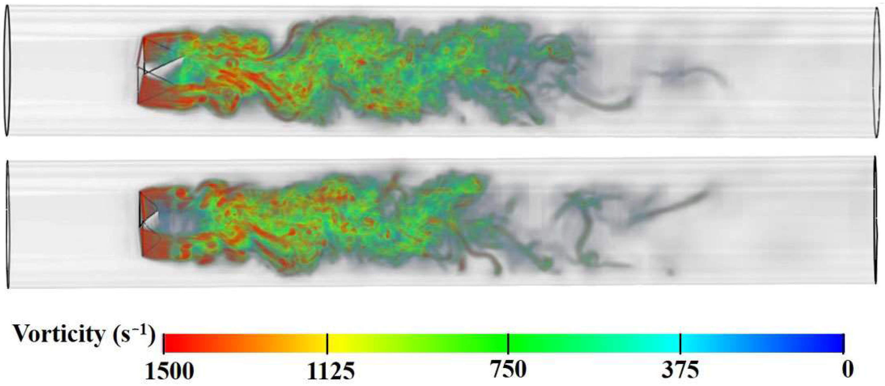
After optimizing the shape of the incoming flow surface, the side, and the end of the vortex generator, the vortex generator with an incoming flow surface of 180°, a curvature radius of the concave arc at the side of 25 mm, and a fillet radius at the end of 4 mm was selected as the optimal shape. However, the vorticity generated by the vortex generator under the 3D condition of the pipeline is quite different from the flow around the cylinder under the 2D condition. The vortex generated by the vortex generator will be disturbed in all directions due to the influence of the boundary layer of the surrounding wall, and the vortex street attenuates rapidly, as shown in Figure 15. Under the 3D condition, the pressure loss and vorticity intensity of two vortex generators affected by gas well production fluctuations at normal and low flow rates were mainly investigated to demonstrate whether the optimized vortex generator can be applied at different Reynolds numbers (6.498 × 10⁵ ≤ Re ≤ 22.597 × 10⁵).

The optimized vortex generator has the same characteristic length as the triangular vortex generator, but the optimized vortex generator has a smaller surface area, so the optimized vortex generator has lower resistance under the same pipeline operating conditions. The pipeline cross sections at 0.19 m (two times the inner diameter of the pipeline) upstream and 0.19 m downstream of two vortex generators were selected as references. At the flow rates of 10.21 m/s (Re = 22.597 × 10⁵) and 2.94 m/s (Re = 6.498 × 10⁵), the pressure difference, vortex street frequency, and symmetry deviation values generated by the two vortex generators are shown in Table 4.

The optimized vortex generator has a vortex street influence area of 0.37 m at a flow rate of 10.21 m/s in the pipeline, and the triangular vortex generator has an influence area of 0.43 m, as shown in Figure 16. The influence areas of vortex generators after and before optimization at the flow rate of 2.94 m/s were 0.26 m and 0.3 2 m, respectively, as shown in Figure 17. It is proved that the optimized vortex generator has less disturbance to the fluid in the pipeline and produces less resistance loss. It is suitable for the lowest value of productivity fluctuation of the gas well and has good energy-saving effect and adaptability.

5. Discussion

Traditional vortex generators (such as cylindrical and trapezoidal) suffer from issues like secondary vortex interference, insufficient vortex strength, and low frequency, with a significant performance decline especially under low flow velocity conditions (in-station pipeline flow velocity less than 5 m/s). Existing research predominantly focuses on two-dimensional simulations and indoor physical experiments, while three-dimensional flow phenomena in real-world applications are more complex, and turbulent flow simulation at high Reynolds numbers remains challenging. This study employs a coupled lattice Boltzmann method (LBM) and large eddy simulation (LES) technique, introducing a dynamic sub-grid-scale stress model (SGS) into the LBM-LES method, which better describes turbulent flow at high Reynolds numbers, providing a numerical simulation foundation for the optimized design of the vortex generator. Under the optimized configuration of a 180° incoming flow surface angle, a 25 mm side concave arc radius, and a 4 mm end fillet radius, the triangular vortex generator exhibits significant multi-dimensional performance enhancements, achieving improved flow field stability, enhanced signal detection accuracy, and optimized vortex structure energy. Specifically, the 180° planar incoming flow design effectively suppresses boundary layer separation, resulting in a pressure loss reduction of approximately 17.2~53.9% compared to the prototype and an increase in vortex shedding frequency of 2.72~13.8%, indicating more regular vortex generation, as shown in

Table 5. Comparison results of the optimized vortex generators at different flow rates under pipeline operating conditions.

Content of Comparison	At 10.21 m/s Triangular Vortex Generator	At 2.94 m/s Triangular Vortex Generator	At 10.21 m/s Optimized Vortex Generator	At 2.94 m/s Optimized Vortex Generator
Pressure drop/Pa	404.54	79.12	334.93	36.51
Lift force per unit area/Pa	max: 248.354 min: −187.831	max: 22.196 min: −22.582	max: 303.126 min: −229.439	max: 26.811 min: −26.477
Frequency/Hz	131.95	32.66	135.55	37.18
Deviation value	0.1387	0.0086	0.1383	0.0062

. Furthermore, the concave arc side profile of the vortex generator reduces the intensity of secondary vortices, providing a flow field basis for high-frequency response vortex detection, while the end fillet design eliminates topological mutations in the vortex morphology at sharp corners, significantly enhancing vortex system symmetry and stability.

However, this study still has certain limitations. For example, in gas pipelines at oil and gas stations, flow velocities are typically controlled within an economic range of 3 to 10 m/s to ensure system economy and efficiency. This research primarily focuses on the optimization design of the vortex generator within this economic flow velocity range (6.498 × 10⁵ ≤ Re ≤ 22.597 × 10⁵), particularly under high Reynolds number conditions. As most high-yield oil fields have entered the later stages of development, low flow conditions will inevitably occur gradually. Therefore, the performance evaluation of vortex flowmeters under low Reynolds number conditions is equally important for future research.

Furthermore, this paper’s simulation assumes the gas to be pure methane, while actual applications may involve the presence of some liquid-phase fluids, which could affect vortex generation and stability. Future research could further explore the optimization of vortex generators under multiphase flow conditions, to clarify the impact of water content on the accuracy of gas measurement by vortex flowmeters.

Additionally, although numerical simulations can provide detailed flow field information and vortex characteristics, the industrial application and promotion of the novel vortex generator still require further validation through experimental data to ensure accuracy and reliability. Currently, the inverse analysis program for high-frequency vortex signals is still under development, which limits the comprehensive evaluation of the optimized vortex generator’s performance in practical applications. Future research will focus on improving this analysis program and experimentally verifying the actual effects of the vortex generator optimization design, aiming to provide more reliable technical support for the industrial application of vortex flowmeters.

6. Conclusions

(1)

The turbulence in 2D and 3D flow fields at high Reynolds numbers can be simulated by the MRT-LBM-LES method, which mainly reveals the instantaneous wake vorticity field, the lift, and the vortex shedding frequency of different forms of vortex generators.

(2)

Various shapes of vortex generators were numerically simulated using the MRT-LBM-LES method in this paper, and a new vortex generator was proposed in the end. Compared with the triangular vortex generator, it is confirmed so that the new vortex generator can produce a strong vortex street at a flow rate of 10.21 m/s (Re = 22.597 × 10⁵) and a low rate of 2.94 m/s (Re = 6.498 × 10⁵).

(3)

The new vortex generator with the inner concave at the side and the fillet at the end can reduce the generation of secondary vortexes and has the advantages of small pressure loss, high vortex frequency, and symmetrical lift.