Self-Organizing Maps-Assisted Variational Autoencoder for Unsupervised Network Anomaly Detection

Abstract

In network intrusion detection systems (NIDS), conventional supervised learning approaches remain constrained by their reliance on labor-intensive labeled datasets, especially in evolving network ecosystems. Although unsupervised learning offers a viable alternative, current methodologies frequently face challenges in managing high-dimensional feature spaces and achieving optimal detection performance. To overcome these limitations, this study proposes a self-organizing maps-assisted variational autoencoder (SOVAE) framework. The SOVAE architecture employs feature correlation graphs combined with the Louvain community detection algorithm to conduct feature selection. The processed data—characterized by reduced dimensionality and clustered structure—is subsequently projected through self-organizing maps to generate cluster-based labels. These labels are further incorporated into the symmetric encoding-decoding reconstruction process of the VAE to enhance data reconstruction quality. Anomaly detection is implemented through quantitative assessment of reconstruction discrepancies and SOM deviations. Experimental results show that SOVAE achieves F1 scores of 0.983 (±0.005) on UNSW-NB15 and 0.875 (±0.008) on CICIDS2017, outperforming mainstream unsupervised baselines.

1. Introduction

The diversity and complexity of cyber-attacks have increased significantly in recent years, which presents significant challenges to network security. Modern cyber-attacks are no longer limited to traditional viruses and worms but also encompass advanced persistent threats (APT), ransomware, phishing, distributed denial of service attacks (DDoS), and zero-day exploit attacks, each characterized by unique tactics, high sophistication, and targeted [1].

In this complex environment, accurately detecting anomalous network traffic presents a critical challenge to network security. Currently, popular network anomaly detection methods include statistical methods, clustering-based methods, and deep-learning-based methods. Statistical methods, such as traditional network anomaly-detection techniques, detect anomalies by evaluating statistical network traffic characteristics. A representative approach is the multivariate statistical network monitoring method based on principal component analysis (PCA) proposed by N. M. Fuentes Garca [2]. This method applies MSPC theory, developed for industrial monitoring, to network monitoring, addressing issues in earlier PCA-based methods, including sensitivity to calibration data and contamination of the normal subspace by large-scale anomalies. However, this method requires extensive data normalization, preprocessing, and alignment depending on the data source and task objectives while exhibiting limited generalization capability.

Cluster-based approaches treat traffic that deviates from known clusters as anomalies. Common clustering algorithms include k-means, DBSCAN, among others. The strengths of clustering methods lie in their ability to identify unknown anomaly patterns and exhibit robust modeling capabilities. However, these methods are often inefficient in high-dimensional and large-scale data scenarios, with sensitivity to parameter selection and initial conditions [3].

In contrast, deep-learning methods can automatically extract intricate features from raw data using multi-layer neural networks, eliminating the need for manual feature engineering. This enables models to effectively handle nonlinear and high-dimensional data, thereby adapting more effectively to complex network traffic patterns and enhancing anomaly detection accuracy [4,5]. For example, Q. P. Nguyen et al. [6] employ variational autoencoders (VAE) combined with gradient-based fingerprinting to construct the GEE network anomaly detection model. It uses VAE to detect anomalies in the dataset and construct a cyber-attack fingerprint based on the gradient change characteristics of the anomalous data. GEE achieves superior overall performance in anomaly detection through the application of fingerprinting techniques. Therefore, a key principle of anomaly detection emerges: compared to normal data points, specific alterations in certain features of anomalous data points result in pronounced variations in the objective function. Consequently, anomaly detection performance can be improved by reducing the noise caused by changes in irrelevant features and highlighting changes in key features.

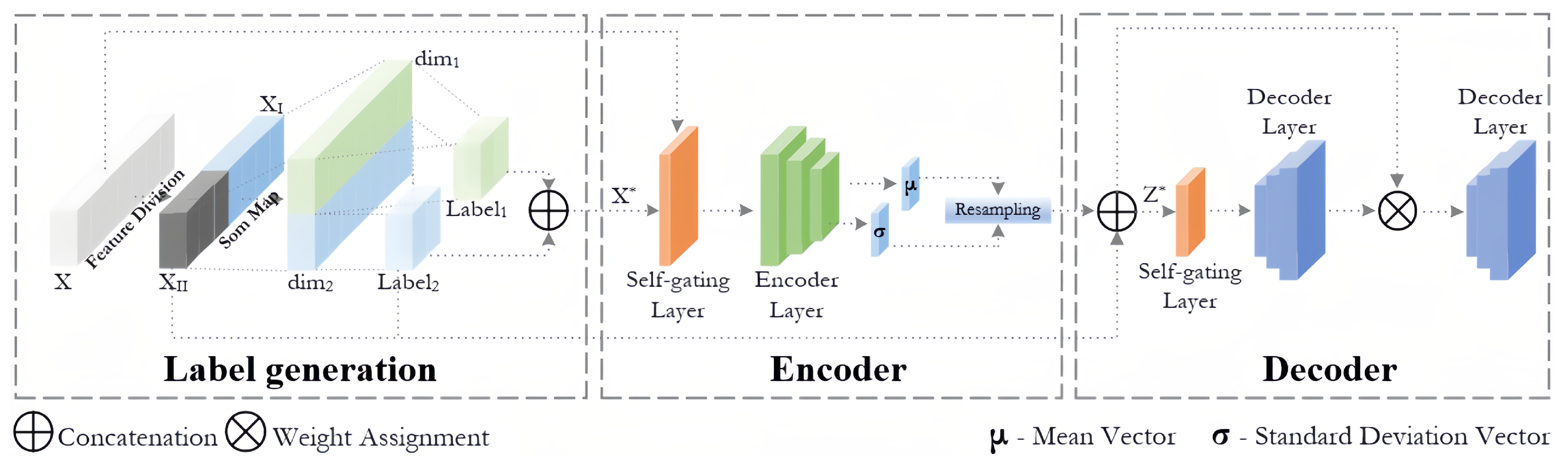
Based on the above ideas, we have constructed a novel unsupervised hybrid model, SOVAE. SOVAE is an unsupervised network anomaly detection model that integrates SOM and VAE. The model partitions data features via a feature correlation graph to reduce feature sparsity. It introduces clustering labels from the SOM into the symmetric “encoder-decoder” network architecture of the VAE to achieve data reconstruction, and incorporates clustering distance to increase the dimensionality of variations in the objective function. The symmetry of the model architecture aids in optimizing the distribution of the latent space, thereby enhancing the robustness of normal pattern reconstruction while amplifying feature deviations in anomalous data. In summary, the main contributions of the research in this paper include:

• We propose a novel unsupervised network anomaly detection model (SOVAE), combining VAE and SOM. The model leverages VAE’s reconstruction error and SOM’s clustering distance to differentiate normal and abnormal samples.
• We carried out ablation experiments, anti-interference experiments, and performance analysis on the UNSW-NB15 [7] and CICIDS2017 [8] datasets, and we studied the effects of feature selection methods based on the feature correlation graph on the mapping accuracy and clustering effect of SOM.

The remainder of this paper is organized as follows: Section 2 reviews related work. Section 3 details the design and implementation of the SOVAE model. Section 4 presents experimental results and performance evaluations. Section 5 concludes the paper and discusses potential directions for future research.

2. Related Work

Deep-learning-based network anomaly-detection methods are typically classified as supervised, semi-supervised, or unsupervised. Supervised methods have significantly addressed data imbalance and enhanced detection accuracy and efficiency. For example, the TMG-GAN model described by H. Ding et al. [9] addresses data imbalance through a multi-generator architecture, classifier design, and cosine similarity loss, outperforming existing algorithms in terms of precision, recall, and F1 score. Semi-supervised methods demand fewer labeled data points compared to their supervised counterparts. A. Hannan et al. [10] introduce a semi-supervised method based on CVAE. This method innovatively encodes normal traffic and malicious traffic into a bimodal distribution in the latent space and optimizes the bimodal representation of the encoder through semi-supervised learning, thereby improving the detection ability of unknown threats.

Unsupervised methods identify patterns and structures by analyzing unlabeled data, offering stronger generalization capabilities and higher practical applicability compared to the other two categories of methods [11]. Current unsupervised anomaly detection methods can be primarily categorized into statistical model-based methods, clustering-based methods, and reconstruction-based methods.

In statistical model-based methods, L. Dinh et al. [12] proposed the RealNVP model, a generative model that employs real-valued non-volume-preserving transformations for density estimation. This model efficiently performs inverse transformations and evaluates the fit of samples to the data distribution by exactly computing the log-likelihood of data points. While RealNVP exhibits strong modeling capabilities, it suffers from complex architecture, high sensitivity to data distributions, and significant computational costs. Zong et al. [13] developed the DAGMM deep-learning model for anomaly detection, which combines deep autoencoders with Gaussian mixture models (GMM). The model first compresses high-dimensional input data into a low-dimensional latent space and then uses GMM to model the data in this latent space. DAGMM demonstrates significant advantages in nonlinear feature learning and multi-modal distribution modeling, making it particularly suitable for unsupervised anomaly detection in high-dimensional and complex data. However, its performance is influenced by reconstruction errors and GMM hyperparameter settings, requiring continuous adjustment based on data feature distributions in practical applications.

In clustering-based methods, G. Pu et al. [14] proposed an unsupervised anomaly detection framework combining subspace clustering (SSC) and one-class support vector machine (OCSVM). This framework reduces data complexity through subspace partitioning and leverages the advantages of OCSVM in one-class classification to enhance the detection of anomalous samples. However, the number of subspaces explodes exponentially with increasing feature dimensions, making computational efficiency a key focus for future optimization. Y. Chen [15] integrated the K-means clustering algorithm with particle swarm optimization (PSO), iteratively optimizing cluster centers and thereby improving the accuracy of data partitioning. This approach outperforms traditional methods in terms of detection accuracy and robustness. Nevertheless, its parameter sensitivity and adaptability to complex scenarios remain primary limitations. Introducing deep-learning methods to strengthen feature representation could enhance the approach’s practical application value.

In reconstruction-based methods, D. Yang et al. [16] proposed a novel anomaly scoring mechanism that combines the reconstruction loss of autoencoders with the Mahalanobis distance of layer outputs, fully utilizing the feature information from the model’s intermediate layers to capture anomalies. On the UNSW-NB15 dataset, this approach significantly outperforms single-method baselines; however, its generalization capability remains insufficiently validated across diverse datasets. Liao et al. [17] developed a hybrid unsupervised framework that integrates multiple deep-learning models and employs Mahalanobis distance to compute reconstruction errors, achieving high anomaly detection accuracy. Nevertheless, its computational overhead and redundancy in certain model components require further optimization. Y. Jiang et al. [18] introduced an anomaly detection method combining VAE and improved K-means clustering. By conducting cluster analysis on samples at the reconstruction threshold boundary, this approach significantly reduces the model’s false alarm rate. However, the manual setting of reconstruction error thresholds and clustering parameters relies on empirical experience, potentially affecting detection performance.

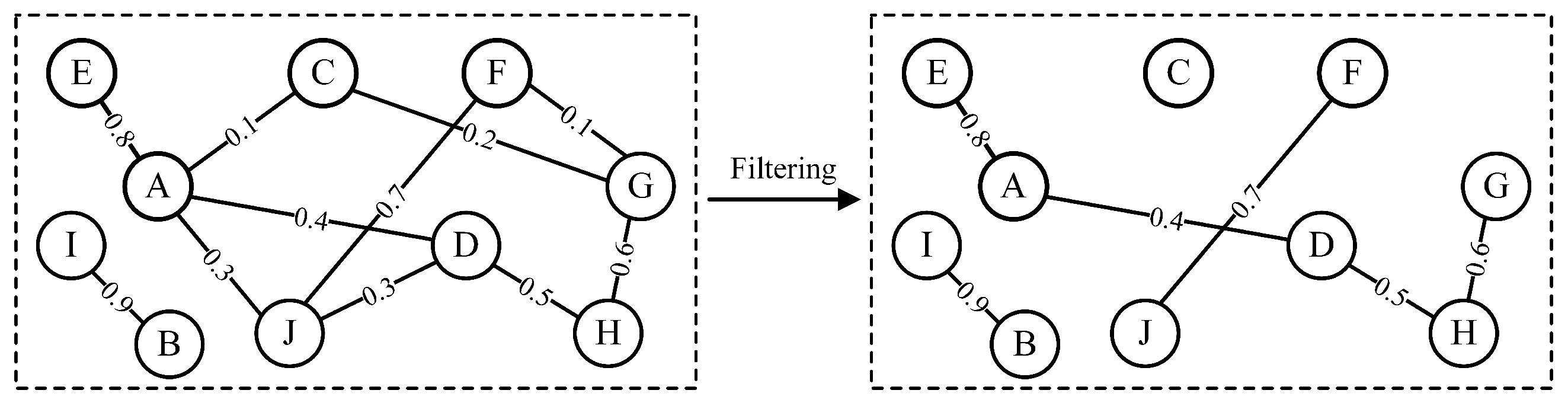
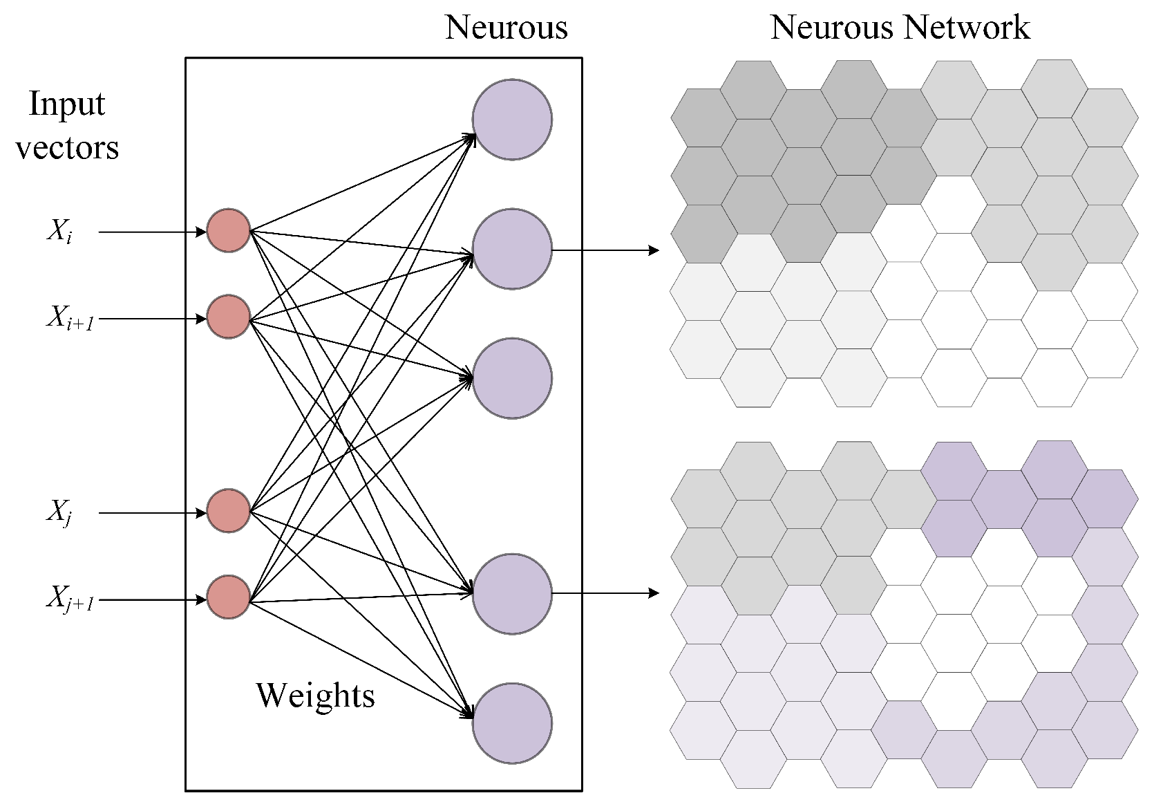
To address the issues of manual setting of cluster numbers and insufficient handling of boundary samples in the above methods, SOVAE automatically generates cluster labels by integrating SOM and incorporates them into the VAE learning process, reducing reliance on manual expertise and strengthening the constraints of the VAE latent space on normal patterns. Furthermore, SOVAE’s dual discriminative metric (reconstruction error and mapping error) offers greater flexibility than a single reconstruction threshold, enhancing robustness in processing boundary samples. Additionally, SOVAE optimizes the input feature space using a feature correlation graph and Louvain algorithm, further improving adaptability to high-dimensional data.

3. Methods

3.1. Overview

We compose the proposed model of two primary components: a SOM network and a VAE. As shown in Figure 1, SOVAE operates through the following steps:

• The input data X are partitioned into normal feature clusters $X_I$ and low-relevance feature clusters $X_{II}$.
• The SOM network maps $X_I$ and $X_{II}$ to distinct dimensions within the neuron network, generating One-Hot labels of the winning neurons for each cluster.
• The VAE splices X with the labels to generate $X^{*}$, which is fed into the encoder. After the resampling stage, $X_{II}$ and the labels are reintroduced to generate the latent representation $Z^{*}$.
• Decoder receives $Z^{*}$ to generate reconstructed samples, and uses the reconstruction error to assign weights to $Z^{*}$ and inputs them to the latter decoder so that it can focus more on those features that are difficult to learn.
• Thresholds for reconstruction error and mapping error are set based on the training data. Then, the samples with reconstruction error or quantization error greater than the threshold are identified as anomalies.

The synergy between SOM and VAE in the model manifests in two aspects:

• Clustering guidance: Through competitive learning, SOM maps high-dimensional data to a low-dimensional topological structure and generates clustering labels. These labels are concatenated with original features during the encoding phase and fused with latent vectors during the decoding phase, forming a symmetric information transmission path. This design constrains the distribution of the VAE’s latent space, compelling it to focus more on the clustering centers of normal data during reconstruction.
• Enhanced anomaly discrimination: Traditional VAE exhibits limited discriminative ability for reconstruction errors of anomalous samples. The cluster center distances provided by SOM, combined with VAE reconstruction errors, form dual discriminative metrics that amplify the degree of deviation in anomalous samples.

3.2. Unsupervised Feature Selection

This section employs the maximal information coefficient (MIC) to assess both linear and nonlinear relationships among network traffic data features. Building upon this analysis, we construct a feature correlation graph and subsequently perform feature selection using the Louvain community detection algorithm.

1.

Maximal information coefficient: MIC is an information theory-based statistic designed to measure the strength of associations between variables, particularly effective at capturing complex linear and nonlinear relationships [19]. The MIC operates within a range of $[0,1]$, where 0 indicates complete statistical independence and 1 represents a perfectly deterministic relationship.

2.

Feature correlation graph: As shown in Figure 2, each node in the graph represents a data feature, and edges connect pairs of feature nodes. The edge weight $W_{ij}$ is determined as Equation (1).

$$W_{ij}=\left\{\begin{array}{cc}{m}_{ij},\hfill & \mathrm{if}{m}_{ij}\ge r,\hfill \\ 0,\hfill & \mathrm{otherwise}\hfill \end{array}\right.$$

(1)

In Equation (1), $m_{ij}$ denotes the MIC between features, and r represents the MIC weight threshold. In this study, r is selected at a level slightly above the dataset mean to preserve statistically significant correlations. This thresholding process constitutes a critical step in balancing information density with noise suppression, effectively eliminating minor relationships that could interfere with analysis. The resulting sparsified graph structure enhances computational tractability while retaining meaningful feature interactions [20].

3.

Louvain algorithm: The Louvain algorithm is a graph community detection method based on modularity optimization. Recognized for its computational efficiency and scalability to large-scale networks, it has become a fundamental tool in graph partitioning [21]. Modularity (Q), a metric quantifying the quality of graph partitioning, is calculated for the feature correlation graph as shown in Equation (2).

$$Q={\displaystyle \frac{1}{2m}}\sum _{ij}\left(W_{ij}-{\displaystyle \frac{k_i{k}_j}{2m}}\right)\delta (c_i,c_j)$$

(2)

In Equation (2), $k_i$ and $k_j$ represent the weighted degrees of nodes i and j, respectively, m is the total edge weight of the graph, and $\delta (c_i,c_j)$ is an indicator function that equals 1 if nodes i and j belong to the same community and 0 otherwise. The modularity value ranges between $[-1,1]$, with higher values indicating denser community structures. The Louvain algorithm iteratively refines graph partitions through a greedy optimization strategy, ultimately converging to a globally optimal community configuration based on modularity maximization. Following multiple executions of the Louvain algorithm to obtain optimal graph partitioning results, we perform dimensionality reduction and feature clustering as follows. Within each community, a subset of features with the highest average correlation coefficients is selected to represent all features in that community. Between communities, isolated communities characterized by low edge weights are identified and aggregated into a low-correlation feature cluster, while the remaining communities form normal feature clusters. This clustering approach reduces data noise, highlights latent features critical for anomaly detection, and enhances the model’s generalization capability [22].

Following the above procedure, the parameter r is set to 1.02 times the mean MIC of the dataset. Features with average MIC values in the top 75% within normal communities are selected to represent the entire community, while the remaining isolated nodes are categorized into low-correlation feature clusters. Taking the UNSW-NB15 dataset as an example, the specific community division results are shown in Figure 3. The normal feature cluster $X_I$ includes features {0, 1, 2, 3, 4, 5, 7, 8, 9, 10, 11, 12, 13, 14, 15, 16, 17, 19, 20, 24, 26, 27, 28, 31, 38, 39, 40}, and the low-correlation feature cluster $X_{II}$ contains features {21, 29, 30, 32, 33, 36, 37}. After dividing the feature clusters, they are respectively input into subsequent models for further processing.

3.3. Self-Organizing Mapping

As shown in Figure 4, The core of a SOM network is a lattice of neurons. The distances between the input sample and all neurons in the network are calculated, typically using the Euclidean distance metric. The neuron with the smallest distance is identified as the best matching unit (BMU) [23]. The updated formula of BMU and Gaussian neighborhood function are defined as Equation (3).

$$W(t+1)=W\left(t\right)+\eta \left(t\right)·H_{ci}\left(t\right)·(X\left(t\right)-W\left(t\right))$$

(3)

In Equation (3), $W\left(t\right)$ is the weight vector of the neuron, $\eta \left(t\right)$ is the learning rate, $H_{ci}\left(t\right)$ is the neighborhood function, and $X\left(t\right)$ is the input sample. The definition of $H_{ci}\left(t\right)$ is given in Equation (4).

$$H_{ci}\left(t\right)=exp\left(-{\displaystyle \frac{d_{ci}^2}{2\sigma {\left(t\right)}^2}}\right)$$

(4)

In Equation (4), $H_{ci}\left(t\right)$ denotes the value of the neighborhood function of the c to the i neuron at time t. $d_{ci}$ is the distance between the BMU and neuronal i. $\sigma \left(t\right)$ is the neighborhood width that decreases with the increase in time t. The Gaussian neighborhood function is a commonly used neighborhood function in SOM, and its exponential decay and dynamic variation in neighborhood width enable SOM to efficiently update and optimize weights while maintaining the data topology [24]. Algorithm 1 illustrates the pseudo-code of the SOM training process. The primary time complexity of the algorithm arises from computing the similarity between the input vectors and the neuronal network, with a complexity of $O(n\times {\dim }_x\times {\dim }_{\mathrm{input}})$, where ${\dim }_x$ is the input vector dimension. The space complexity is mainly determined by the weight matrix W, so the space complexity is $O({\dim }_x\times {\dim }_{\mathrm{input}})$.

Algorithm 1 Self-Organizing Map

1: function SOM_Train($f_{\mathrm{neighbors}}$, ${\eta }_{\mathrm{SOM}}$,${\mathit{dim}}_x$, ${\mathit{dim}}_{\mathit{input}}$, D) 2:     Initialize W #Randomly selecting vector from D to Initialize the weight vectors of nodes in a feature map 3:     for each epoch do 4:         Select an input vector $D\left(t\right)$ from D 5:         $dis\leftarrow \mathrm{None}$ 6:         for each neuron $v\in \{1,2,\dots ,{\mathit{dim}}_x\}$ do 7:            if $dis==\mathrm{None}$ then 8:                $dis\leftarrow d(D\left(t\right)-W_v\left(e\right)$ #Update the activation distance for v 9:            else 10:                if $d\left(D\right(t)-W(v\left)\right)<dis$ then 11:                    $dis\leftarrow d(D\left(t\right)-W_v\left(e\right))$ 12:                    $u\leftarrow v$ #Update the BMU for $D\left(t\right)$ 13:                end if 14:            end if 15:         end for 16:         for each neuron v do 17:            $W_v(e+1)\leftarrow W_v\left(e\right)+f_{\mathrm{neighbor}}(u,v,e)·{\eta }_{\mathrm{SOM}}·\mathrm{Scheduler}\left(e\right)·(D\left(t\right)-W_v\left(e\right))$ #Update the BMU and the neighbor nodes 18:         end for 19:     end for 20:     return W 21: end function

3.4. Variational Autoencoder

The VAE loss function comprises two components: the reconstruction error and the distribution error. The reconstruction error is composed of the reconstruction error $E_1$ of decoder 1 and the reconstruction error of decoder 2 $E_2$. The distribution error uses the KL divergence to measure the difference between the approximate distribution $q_{\varphi }\left(z\right|x)$ and the prior distribution $p\left(z\right)$. In summary, the loss function of VAE is given in Equation (5).

$$l_{\mathrm{VAE}}=E_1\left[\parallel X-X^{\prime }{\parallel }^2\right]+E_2\left[W_{e_1}\times {\parallel X-X^{\prime }\parallel }^2\right]+\beta ·\mathrm{KL}\left(N(z_{\mu },z_{\sigma })\Vert N(0,1)\right)$$

(5)

In Equation (5), the reconstruction errors E are all computed using the mean square error. $W_{E_1}$ is the weight vector determined by the reconstruction error $E_1$, and samples with large reconstruction errors in $E_1$ have higher weights in the loss function. $\beta$ is the hyperparameter that adjusts the KL scatter. Algorithm 2 shows the pseudo-code of the VAE training procedure. In this case, the encoder and decoder are fully connected networks with a total of L layers of the network, and the complexity of each layer is $O({\dim }_{\mathrm{input}}\times {\dim }_{\mathrm{latent}})$, so the algorithm time complexity is roughly $O(n\times {\sum }_{i=1}^L{\dim }_{{\mathrm{input}}_{\mathrm{i}}}\times {\dim }_{{\mathrm{latent}}_{\mathrm{i}}})$, and the space complexity is $O({\sum }_{i=1}^L{\dim }_{{\mathrm{input}}_{\mathrm{i}}}\times {\dim }_{{\mathrm{latent}}_{\mathrm{i}}})$.

Algorithm 2 Variational Autoencoders

1: function VAE_Train($X_I,X_{II},\mathrm{label},\rho$) 2:     Initialize Parameters # ${\dim }_{\mathrm{input}},{\dim }_{\mathrm{latent}},{\dim }_{VAE}$ 3:     for each epoch e do 4:         $\mu ,\sigma \leftarrow \mathrm{Encoder}(X_I,X_{II},\mathrm{label})$ # Get potential spatial parameters 5:         $z\leftarrow \mu +e^{\sigma /2}·\mathrm{Randn}\_\mathrm{like}\left(\sigma \right)$ # reparameterize 6:         $X{r}_1\leftarrow {\mathrm{Decoder}}_1(X_I,X_{II},\mathrm{label})$ 7:         $X{r}_2\leftarrow {\mathrm{Decoder}}_2(z,X_I,\mathrm{label})$ 8:         $W_{E_1}\leftarrow \mathrm{Get}\_\mathrm{weight}(X_I,X{r}_1,\rho )$ 9:         ${\mathrm{loss}}_{r1},{\mathrm{loss}}_{r2},{\mathrm{loss}}_{KL}\leftarrow \mathrm{Loss}(X{r}_1,X{r}_2,X_I,W_{E_1},\mu ,\sigma )$ 10:         $\mathrm{Backward}({\mathrm{loss}}_{r1}+{\mathrm{loss}}_{r2}+\beta ·{\mathrm{loss}}_{KL})$ 11:     end for 12: end function 13: function Get_weight($X_I,X_r,\rho$) 14:     $mse\leftarrow \mathrm{Mse}\_\mathrm{loss}(X_I,X_r)$ 15:     if $mse>{\mathrm{mse}}_{\mathrm{mean}}·\rho$ then 16:         $w_i\leftarrow \mathrm{Max}\_\mathrm{Min}\_\mathrm{Scale}\left(mse\right)$ # After removing several maximum values, scale mse to $(0,1)$ 17:     else 18:         $w_i\leftarrow \mathrm{None}$ 19:     end if 20:     return w 21: end function

4. Results

4.1. Dataset and Experimental Setup

4.1.1. UNSW-NB15

The UNSW-NB15 dataset is a dataset for network intrusion detection systems developed by the University of New South Wales (UNSW) in collaboration with the Australian Centre for Cyber Security. The dataset was released in 2015 to fill the gaps in diversity and feature completeness of existing network intrusion detection datasets [4]. The dataset includes 49 features and one label field, encompassing basic, content-based, temporal, and traffic-related attributes, and is capable of being used to identify normal traffic as well as specific types of attack traffic.

This dataset generates real network traffic data in a virtual network through the IXIA PerfectStorm tool, which provides rich attack traffic samples and is widely used in network security research. The distribution of the UNSW-NB15 test set is presented in

Table 1. Distribution of the test set of UNSW-NB15.

Network Type	Number of Data Points	Percentage (%)
Benign	665,630	87.351
Generic	64,644	8.483
Exploits	13,358	1.753
Fuzzers	7274	0.955
DoS	4906	0.644
Reconnaissance	4196	0.551
Analysis	803	0.105
Backdoor	699	0.092
Shellcode	453	0.059
Worms	52	0.007

.

4.1.2. CICIDS2017

The CICIDS2017 dataset was developed by the Canadian Institute of Cybersecurity to provide a representative network traffic dataset for research on network intrusion detection systems [5]. The CICIDS2017 dataset has more than 80 features that were extracted from the generated network traffic by using the CICFlowMeter tool, containing the complete packet payload (in pcap format), the corresponding traffic features, and the labeled traffic records.

Table 2. Distribution of the test set of CICIDS2017.

Network Type	Number of Data Points	Percentage (%)
Benign	678,109	80.331
DoS Hulk	68,760	8.146
PortScan	47,311	5.605
DDoS	38,125	4.516
DoS GoldenEye	3087	0.366
FTP-Patator	2368	0.281
SSH-Patator	1758	0.208
DoS Slowloris	1731	0.205
DoS Slowhttptest	1646	0.195
Bot	583	0.069
Web Attack Brute Force	449	0.053
Web Attack XSS	194	0.023
Infiltration	10	0.001
Web Attack Sql Injection	6	0.001
Heartbleed	3	0.001

lists the distribution of the CICIDS2017 test set.

4.1.3. Experimental Setup

The experimental machine is configured with Windows 10 as the operating system, an i5-12490F CPU @ 3 GHz (Intel Corporation, Santa Clara, CA, USA), NVIDIA GeForce RTX 3070 Graphics Card (Micro-Star International Co., Ltd., New Taipei City, Taiwan, China), and 64 GB RAM (Kingston Technology Company, Inc., Fountain Valley, CA, USA). The software environment includes Python 3.9 and PyTorch 2.0.1 + cu118.

Parameter configuration: The resolution parameter in the Louvain algorithm is set to 0.9 to prioritize the merging of sparsely connected small communities. SOM employs a Gaussian neighborhood function with an initial learning rate of $1\times {10}^{-5}$, trained for 20 epochs per iteration. VAE processes input data through fully connected layers and LeakyReLU activation functions in both its encoder and decoder. The initial learning rate is $6\times {10}^{-3}$, with a learning rate decay step of 25 and a decay coefficient of 0.98. Each training session consists of 150 rounds. This configuration balances algorithmic specificity with computational efficiency while maintaining convergence stability across modules.

4.2. Evaluate Metrics

4.2.1. Clustering Quality

Quantization error is a critical metric for evaluating clustering quality, particularly in SOM and other neural network-based methods. It measures the distance between data points and their corresponding mapped positions, and the smaller the distance, the better the tightness and accuracy of clustering [25], which is calculated as follows:

$$QE=\sum _{i=1}^k\sum _{x\in C_i}{\parallel x-{\mu }_i\parallel }^2$$

(6)

where k is the number of neurons, $C_i$ is the i neuron, x is the data point mapped to the neuron, and ${\mu }_i$ is the weight vector of the neuron.

4.2.2. Anomaly Detection

The average precision, recall, and F1 score are intuitive metrics for comparing anomaly detection performance. Precision measures the proportion of instances correctly identified as positive out of all instances predicted to be positive by the model. Recall represents the proportion of actual positive instances correctly identified by the model. These metrics are defined as follows:

$$\mathrm{Precision}={\displaystyle \frac{TP}{TP+FP}},\mathrm{Recall}={\displaystyle \frac{TP}{TP+FN}}$$

where TP is the number of true positive samples, FP is the number of false positive samples, and FN is the number of false negative samples. the F1 score is the reconciled average of the precision checking rate and recall rate, which integrates the precision checking rate and recall rate of the model, and it is especially useful in the case of unbalanced data. The formula is as follows:

$$F1={\displaystyle \frac{2\times \mathrm{Precision}\times \mathrm{Recall}}{\mathrm{Precision}+\mathrm{Recall}}}$$

4.3. Outcome

4.3.1. Model Comparison

In the scenarios where only unlabeled normal data are utilized as training data, the experimental results for both datasets are presented in

Table 3. Performance metrics comparison across different methods for the UNSW-NB15 and CICIDS2017 datasets.

Method	UNSW-NB15			CICIDS2017
	Prec.	Recall	F1 Score	Prec.	Recall	F1 Score
REALNVP [12]	0.892	0.861	0.876	0.779	0.783	0.781
WGAN [26]	0.885	0.884	0.885	0.813	0.687	0.718
ENAD [17]	0.979	0.924	0.941	0.838	0.840	0.835
DAGMM [13]	0.535	0.527	0.531	0.764	0.765	0.765
DAE	0.959	0.969	0.962	0.810	0.826	0.814
VAE	0.722	0.747	0.734	0.745	0.682	0.712
GAN	0.808	0.864	0.823	0.673	0.803	0.715
IF	0.950	0.927	0.933	0.837	0.845	0.816
SOVAE	0.985	0.983	0.983	0.874	0.876	0.875

. Among them, DAE stands for the denoising autoencoder, VAE is the standard variational autoencoder, IF stands for the isolation forest algorithm and GAN is the generative adversarial network. It can be observed that, in the UNSW-NB15 dataset, SOVAE surpasses the best benchmark method by approximately 2% in both recall and F1 score, while achieving the highest model accuracy. Similarly, in the CICIDS2017 dataset, SOVAE exceeds the performance of the best benchmark method by approximately 3.5% across all metrics. The experimental results from both datasets demonstrate that the proposed model is capable of more clearly separating normal and abnormal data within the latent space. Furthermore, it is evident that intrusion detection in the CICIDS2017 dataset presents greater complexity and challenges, as it is lower than the results of the UNSW-NB15 dataset in almost all evaluation metrics.

Figure 5 illustrates the results of the clustering experiment, where Raw represents the original dataset. These experiments employed the same SOM structure and hyperparameter configurations to evaluate the impact of the feature selection method on SOM’s clustering performance. As a comparison, we introduced principal component analysis (PCA) and autoencoder (AE) methods to test the downscaling and dimensioning of the dataset. The reported results are averaged from multiple experimental runs.

4.3.2. Performance Analysis

As shown in Figure 6, on the UNSW-NB15 dataset, SOVAE exhibited high classification robustness. Specifically, it achieved a false positive rate of 1.50% and a false negative rate of 1.67%, indicating extremely low misjudgment probabilities for both normal and anomalous samples. However, on the CICIDS2017 dataset, SOVAE’s misclassification rate increased significantly. The false positive rate reached 6.73%, and notably, the false negative rate surged to 29.66%, highlighting limitations in its cross-scenario generalization capability. The CICIDS2017 dataset features higher dimensionality and includes more novel attack patterns, with substantial overlap between attack traffic and normal traffic, making it difficult for SOVAE to capture critical discriminative features. We propose that in future work, generative models (e.g., GANs) could be integrated to augment overlapping traffic, enhance SOVAE’s discriminative ability, and reduce the false negative rate.

Additionally, the response of SOVAE to contaminated training data was investigated under the same parameter settings. Abnormal data samples were randomly selected and combined with normal data to create training datasets with varying proportions of contamination.

Table 4. Average precision, recall and F1 score from SOVAE with different noise ratios (the ratio c represents the proportion of anomalous samples in the training data).

Ratio c	UNSW-NB15			CICIDS2017
	Prec.	Recall	F1 Score	Prec.	Recall	F1 Score
0%	0.985	0.983	0.983	0.874	0.876	0.875
1%	0.969	0.961	0.963	0.870	0.872	0.871
3%	0.965	0.954	0.957	0.844	0.849	0.847
5%	0.943	0.900	0.911	0.830	0.841	0.833

illustrates the impact of different contamination levels on SOVAE’s performance across the two datasets. When the proportion of abnormal data escalates from 0% to 5%, all the accuracy, recall, and the F1 score of SOVAE exhibit a descending trend. Therefore, our subsequent research will prioritize enhancing the robustness of SOVAE while continuing to strengthen its anomaly detection capabilities, thereby ensuring effective adaptation to dynamic and heterogeneous real-world network environments.

4.3.3. Ablation Study

The ablation study results of the SOVAE model presented in

Table 5. Average F1 score from SOVAE in ablation experiments. (A checkmark indicates the module is enabled in SOVAE.)

VAE	SOM	FS	F1 Score
			UNSW-NB15	CICIDS2017
√			0.745	0.729
	√		0.917	0.724
√	√		0.941	0.826
√		√	0.939	0.737
	√	√	0.965	0.755
√	√	√	0.983	0.875

indicate that synergistic effects between modules significantly impact model performance. Specifically, the combination of VAE and SOM achieves notable performance improvements on both the UNSW-NB15 and CICIDS2017 datasets, with a 14.2% enhancement over single modules on CICIDS2017, validating the synergistic advantages of feature learning and clustering optimization. The VAE–feature selection (FS) combination exhibits dataset dependency: it improves performance by 26% on UNSW-NB15 but only by 1.1% on CICIDS2017, suggesting that high-dimensional complex data impose greater demands on the adaptability of feature optimization strategies. In contrast, the SOM-FS combination achieves stable improvements of 5.2% and 4.3% on the two datasets, demonstrating that feature selection offers more generalized robustness in optimizing clustering performance.

Ultimately, the full model integrating VAE, SOM, and FS achieves optimal performance on both datasets. Particularly in the complex network attack scenario of CICIDS2017, the multi-module synergy strategy—through the organic integration of feature learning, clustering optimization, and data dimensionality reduction—significantly enhances detection performance, further confirming the complementarity of the module design. This study not only validates the effectiveness of the SOVAE model but also provides critical insights for optimizing feature selection modules in high-dimensional data scenarios.

5. Discussion

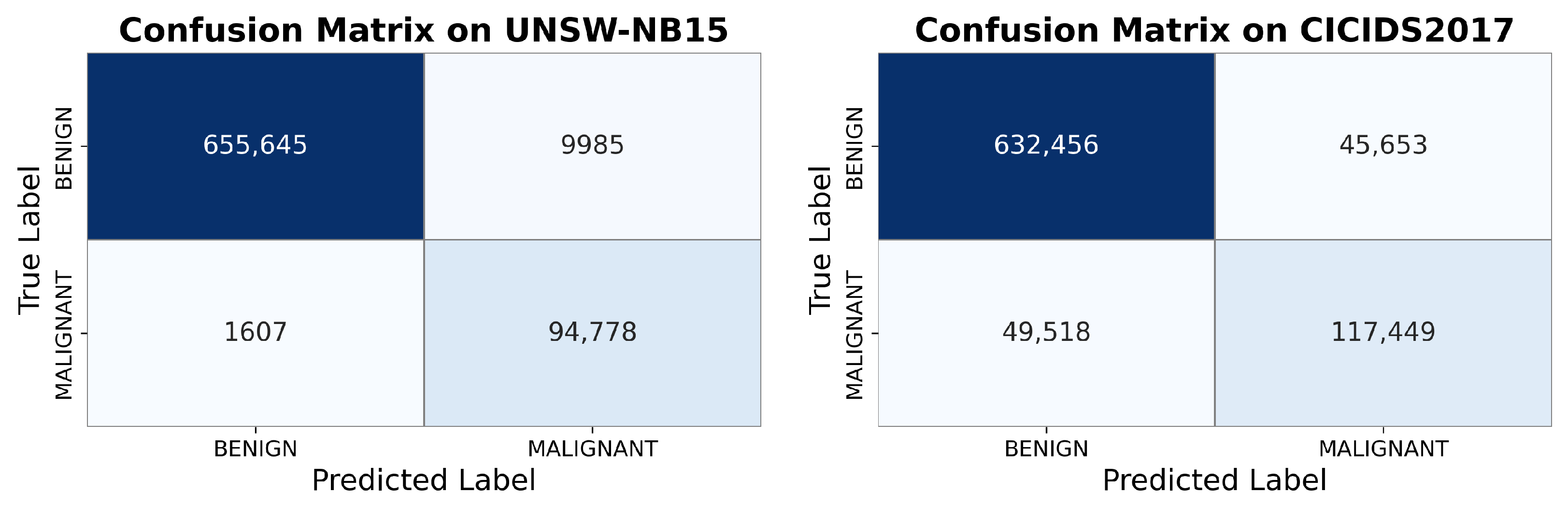
This study proposes an unsupervised network anomaly detection model named SOVAE, based on self-organizing maps (SOM) and variational autoencoders (VAE). The model distinguishes normal and anomalous samples by leveraging the reconstruction error of VAE and the mapping distance of SOM. Experimental results demonstrate that SOVAE achieves F1 scores of 0.983 and 0.875 on the UNSW-NB15 and CICIDS2017 datasets, respectively, outperforming current mainstream unsupervised methods.

The core innovation of SOVAE lies in its feature processing method and model architecture design. Feature selection based on a feature correlation graph significantly improves the clustering quality of SOM; the symmetric encoder-decoder architecture and bidirectional information flow enhance the reconstruction accuracy of normal features and the sensitivity of anomaly discrimination. Ablation experiments further validate the contribution of each component to the overall performance, with results showing that the introduction of feature selection and soft labels significantly enhances the model’s detection capability. However, this study still has the following limitations:

• Insufficient adaptability to complex attack patterns: On the CICIDS2017 dataset, due to the high feature overlap between attack traffic and normal traffic and the inclusion of more novel attack patterns, the model’s misdetection rate increased significantly (e.g., the false negative rate reached 29.66%), indicating that its generalization capability to unknown attack types requires improvement.
• Sensitivity to data contamination: Experimental results demonstrate that when the proportion of anomalous samples in the training data increases, the model’s performance significantly degrades, indicating that its robustness requires further optimization.

In future research, generative models such as GANs could be introduced to perform data augmentation on overlapping traffic, improving the model’s discriminative ability for complex attack patterns. Additionally, the development of dynamic threshold adjustment mechanisms or ensemble learning frameworks could enhance the model’s robustness in scenarios with data contamination. Overall, SOVAE demonstrates significant potential in the field of unsupervised network anomaly detection. By addressing existing limitations and integrating emerging technologies, this model is poised to play a broader role in dynamic and complex network environments.

References

1. Aslan, Ö.; Aktuğ, S.S.; Ozkan-Okay, M.; Yilmaz, A.A.; Akin, E. A comprehensive review of cyber security vulnerabilities, threats, attacks, and solutions. Electronics 2023, 12, 1333. [Google Scholar] [CrossRef]
2. Fuentes García, N.M. Multivariate Statistical Network Monitoring for Network Security Based on Principal Component Analysis. 2021. Available online: https://digibug.ugr.es/handle/10481/67941 (accessed on 1 December 2024).
3. Pang, G.; Shen, C.; Cao, L.; Hengel, A.V.D. Deep learning for anomaly detection: A review. ACM Comput. Surv. (CSUR) 2021, 54, 1–38. [Google Scholar] [CrossRef]
4. Chalapathy, R.; Chawla, S. Deep learning for anomaly detection: A survey. arXiv 2019, arXiv:1901.03407. [Google Scholar]
5. Hodge, V.; Austin, J. A survey of outlier detection methodologies. Artif. Intell. Rev. 2004, 22, 85–126. [Google Scholar]
6. Nguyen, Q.P.; Lim, K.W.; Divakaran, D.M.; Low, K.H.; Chan, M.C. Gee: A gradient-based explainable variational autoencoder for network anomaly detection. In Proceedings of the 2019 IEEE Conference on Communications and Network Security (CNS), Washington, DC, USA, 10–12 June 2019; pp. 91–99. [Google Scholar]
7. Moustafa, N.; Slay, J. UNSW-NB15: A comprehensive data set for network intrusion detection systems (UNSW-NB15 network data set). In Proceedings of the 2015 Military Communications and Information Systems Conference (MilCIS), Canberra, Australia, 10–12 November 2015; pp. 1–6. [Google Scholar]
8. Sharafaldin, I.; Lashkari, A.H.; Ghorbani, A.A. Toward generating a new intrusion detection dataset and intrusion traffic characterization. ICISSp 2018, 1, 108–116. [Google Scholar]
9. Ding, H.; Sun, Y.; Huang, N.; Shen, Z.; Cui, X. TMG-GAN: Generative adversarial networks-based imbalanced learning for network intrusion detection. IEEE Trans. Inf. Forensics Secur. 2023, 19, 1156–1167. [Google Scholar]
10. Hannan, A.; Gruhl, C.; Sick, B. Anomaly based resilient network intrusion detection using inferential autoencoders. In Proceedings of the 2021 IEEE International Conference on Cyber Security and Resilience (CSR), Rhodes, Greece, 26–28 July 2021; pp. 1–7. [Google Scholar]
11. Naeem, S.; Ali, A.; Anam, S.; Ahmed, M.M. An unsupervised machine learning algorithms: Comprehensive review. Int. J. Comput. Digit. Syst. 2023, 13, 911–921. [Google Scholar]
12. Dinh, L.; Sohl-Dickstein, J.; Bengio, S. Density estimation using real nvp. arXiv 2016, arXiv:1605.08803. [Google Scholar]
13. Zong, B.; Song, Q.; Min, M.R.; Cheng, W.; Lumezanu, C.; Cho, D.; Chen, H. Deep autoencoding gaussian mixture model for unsupervised anomaly detection. In Proceedings of the International Conference on Learning Representations, Vancouver, BC, Canada, 30 April–3 May 2018. [Google Scholar]
14. Pu, G.; Wang, L.; Shen, J.; Dong, F. A Hybrid Unsupervised Clustering-Based Anomaly Detection Method. Tsinghua Sci. Technol. 2021, 26, 146–153. [Google Scholar]
15. Chen, Y. Construction of a computer network fault analysis and intrusion detection system based on K-means clustering algorithm. In Proceedings of the 2023 8th International Conference on Information Systems Engineering (ICISE), Dalian, China, 23–25 June 2023; pp. 70–75. [Google Scholar]
16. Yang, D.; Hwang, M. Unsupervised and ensemble-based anomaly detection method for network security. In Proceedings of the 2022 14th International Conference on Knowledge and Smart Technology (KST), Chon buri, Thailand, 26–29 January 2022; pp. 75–79. [Google Scholar]
17. Liao, J.; Teo, S.G.; Kundu, P.P.; Truong-Huu, T. ENAD: An ensemble framework for unsupervised network anomaly detection. In Proceedings of the 2021 IEEE International Conference on Cyber Security and Resilience (CSR), Rhodes, Greece, 26–28 July 2021; pp. 81–88. [Google Scholar]
18. Jiang, Y.; Huang, T.; Wang, J.; Kang, C. Anomaly detection of Argo data using variational autoencoder and K-means clustering. In Proceedings of the 2022 IEEE 5th Advanced Information Management, Communicates, Electronic and Automation Control Conference (IMCEC), Chongqing, China, 16–18 December 2022; pp. 1000–1004. [Google Scholar]
19. Reshef, D.N.; Reshef, Y.A.; Finucane, H.K.; Grossman, S.R.; McVean, G.; Turnbaugh, P.J.; Lander, E.S.; Mitzenmacher, M.; Sabeti, P.C. Detecting novel associations in large data sets. Science 2011, 334, 1518–1524. [Google Scholar] [PubMed]
20. Chen, T.; Deng, G. Model-Free Feature Screening via Maximal Information Coefficient (MIC) for Ultrahigh-Dimensional Multiclass Classification. Open J. Stat. 2023, 13, 917–940. [Google Scholar] [CrossRef]
21. Blondel, V.D.; Guillaume, J.L.; Lambiotte, R.; Lefebvre, E. Fast unfolding of communities in large networks. J. Stat. Mech. Theory Exp. 2008, 2008, P10008. [Google Scholar]
22. Liu, J.B.; Zheng, Y.Q.; Lee, C.C. Statistical analysis of the regional air quality index of Yangtze River Delta based on complex network theory. Appl. Energy 2024, 357, 122529. [Google Scholar] [CrossRef]
23. Wang, R.; Shi, T.; Zhang, X.; Wei, J.; Lu, J.; Zhu, J.; Wu, Z.; Liu, Q.; Liu, M. Implementing in-situ self-organizing maps with memristor crossbar arrays for data mining and optimization. Nat. Commun. 2022, 13, 2289. [Google Scholar] [CrossRef] [PubMed]
24. Chen, Y.; Ashizawa, N.; Yeo, C.K.; Yanai, N.; Yean, S. Multi-scale self-organizing map assisted deep autoencoding Gaussian mixture model for unsupervised intrusion detection. Knowl. Based Syst. 2021, 224, 107086. [Google Scholar] [CrossRef]
25. Hameed, A.A.; Jamil, A.; Alazzawi, E.M.; Marquez, F.P.G.; Fitriyani, N.L.; Gu, Y.; Syafrudin, M. Improving the performance of self-organizing map using reweighted zero-attracting method. Alex. Eng. J. 2024, 106, 743–752. [Google Scholar]
26. Arjovsky, M.; Chintala, S.; Bottou, L. Wasserstein generative adversarial networks. In Proceedings of the International Conference on Machine Learning, Sydney, Australia, 6–11 August 2017; pp. 214–223. [Google Scholar]
Figure 1. Overview of the SOVAE.
Symmetry 17 00520 g001
Figure 2. Feature correlation graph.
Symmetry 17 00520 g002
Figure 3. Louvain community detection graph on the UNSW-NB15 (Nodes of the same color belong to the same community).
Symmetry 17 00520 g003
Figure 4. Overview of self-organizing mapping.
Symmetry 17 00520 g004
Figure 5. Impact of feature selection on Quantization Error of SOM (Raw—raw data; PCA—principal component analysis; AE—autoencoder dimensionality reduction).
Symmetry 17 00520 g005
Figure 6. SOVAE confusion matrix (UNSW-NB15: FPR-1.50%, FNR-1.67%; CICIDS2017: FPR-6.73%, FNR-29.66%).
Symmetry 17 00520 g006