Bluff Body Size Parameters and Vortex Flowmeter Performance: A Big Data-Based Modeling and Machine Learning Methodology

Abstract

This study investigates the correlation between bluff body parameters and vortex flowmeter performance through big data modeling and machine learning techniques. Vortex flowmeters are widely used in industry due to their high accuracy and minimal pressure loss. Nonetheless, optimizing their design remains challenging due to the complex relationship between input and output parameters. Symmetry in bluff body design is crucial for vortex formation and stability. In this study, Latin Hypercube Sampling (LHS) was employed to generate 10,000 symmetry bluff bodies, and efficient serial simulations were conducted using Ansys Fluent, significantly reducing computational costs compared to traditional CFD methods. A regression model was developed using scikit-learn to map eight geometric parameters to eight performance indicators, achieving excellent fitting accuracy with residuals far smaller than the simulation accuracy of ANSYS Fluent. Through Grey Relational Analysis (GRA), objective function analysis, and in conjunction with CFD contour maps, this study has analyzed the relationships between input and output parameters and their impact on the Karman vortex street. This work has significantly improved the speed of big data collection and provided a solid theoretical foundation for data-driven optimization through big data analysis. In addition, the improvement of existing machine learning methods has achieved high-precision prediction and system parameter optimization, promoting the design of vortex flowmeters.

1. Introduction

Under specific flow conditions, when a fluid medium passes through a bluff body, regular vortices alternate behind the bluff body, a phenomenon known as the Karman vortex street. The concept of symmetry plays a vital role in understanding this phenomenon. Symmetry in the geometric configuration of bluff bodies can significantly influence the formation and stability of vortices. In 1912, Von Kármán [1] studied the stability of vortex streets, laying the theoretical foundation for vortex flowmeters. In industrial production, vortex flowmeters have the advantages of a simple, straight-curve structure, wide application range, and long service life.

Early experimental [2,3] and theoretical studies [4,5,6] have laid the foundation for this field. In 2004, the CFD method was introduced for simulation for the first time [7]. In 2011, Venugopal et al. [8] determined the best blocking ratio (d/D) for bluff bodies to be 0.28 through experiments. Du Peng [9] conducted numerical simulations in 2015, proposing the optimal bluff body shapes for Newtonian and power-law fluids, respectively. Venugopal et al. [10] proposed in 2019 that trapezoidal bluff bodies generate vortices with significant two-dimensional characteristics under stable turbulence, making them the most suitable shape. Krivonogov et al. [11] established a simulation system in 2020 that converts two-dimensional signals into three-dimensional vortex streets. Rzasa et al. [12] conducted simulations and experiments in 2021, concluding that a streamlined upstream side stabilizes the vortex street at high flow rates, while a sharp downstream edge enhances flowmeter sensitivity. Končar et al. [13] used OpenFOAM in 2022 to simulate Reynolds numbers between 8300 and 50,000, achieving good results with DNS, LES, and URANS methods, particularly URANS in the low Reynolds number region. Shen [14] determined the optimal pressure measurement point for vortex flowmeters using CFX in 2023. Lur’e [15] optimized the bluff body shape in 2024, improving the sensitivity and accuracy of vortex oscillation sensors in submersible flowmeters. Farsad [16] utilized wind tunnel experiments in 2025 to study the downstream flow characteristics of five distinct bluff body geometries. Although the influence laws of key parameters such as blockage ratio and streamlined design of flow surface have been proposed, most studies are still limited to simulation analysis of single or few shapes, lacking systematic modeling of multi-parameter synergistic effects and simulation of non-traditional shaped bluff bodies.

In recent years, with the rapid development of big data and machine learning technologies, their applications in the industrial field have become increasingly widespread. Especially in complex system optimization, machine learning algorithms have demonstrated powerful capabilities. For example, Zhang et al. proposed an improved deep reinforcement learning algorithm for solving parallel machine scheduling problems with different delivery time constraints in multiple scenarios [17]. Moreover, Ren et al. proposed an efficient m-step look-ahead rollout algorithm to address the profit-oriented selective disassembly sequence planning problem with stochastic operation failures, significantly enhancing both the solution quality and computational efficiency [18]. In the design and optimization of vortex flowmeters, the system has multiple input–output parameters, and similar machine-learning methods have shown great potential. In addition, the cross-application of machine learning and computational fluid dynamics has provided new ideas for structural optimization, which have been applied in turbulence [19,20,21,22], flow control [23,24,25,26,27,28,29,30], and aerodynamics [27,28,29,31]. Machine learning methods can be roughly divided into three categories: data-driven substitution, physical information substitution, and machine learning-assisted numerical solutions. Data-driven agents rely solely on observational data to train algorithms capable of simulating complex fluid dynamics. The physics-informed surrogate integrates the selected physics-informed priors into machine-learning modeling. Machine learning-assisted numerical solutions have partially replaced traditional numerical solvers, achieving a balance between efficiency, accuracy, and generalization. However, the application of these methods in the field of vortex flowmeters is still in the exploratory stage, especially in the multi-objective optimization of geometric parameters, and there is no systematic method yet. Thummar et al. first used machine learning to optimize the structure of bluff bodies in 2022 [32]. Unfortunately, existing methods have not established clear correlations between shape, size, and specific output parameters, resulting in design optimization relying on empirical trial and error, which is inefficient. Due to the need for big data support in this field, current research is insufficient.

Scikit-learn is one of the most popular machine learning libraries in Python, providing a wealth of algorithms and tools for building, evaluating, and optimizing predictive models. In recent years, researchers have made remarkable achievements in many fields by using the scikit-learn library: Sudharsan B et al. [33] and Georg et al. [34] used machine learning techniques such as random forest, K-nearest neighbor, naive Bayes, and support vector machine (SVM) to predict hypoglycemia in patients with type 2 diabetes. The research results indicate that these models can effectively predict hypoglycemic events, providing strong support for clinical decision-making. This demonstrates the powerful predictive ability of scikit-learn for models under the influence of complex factors. This article proposes an innovative approach that combines serial simulation technology with machine learning to systematically analyze the correlation between bluff body geometry parameters and vortex flowmeter performance. A dataset of 10,000 geometric configurations was generated using Latin Hypercube Sampling (LHS), and efficient serial simulations were conducted using Ansys Fluent 2023R1, resulting in a 50% reduction in computational cost compared to traditional CFD methods. An improved machine learning model was developed using scikit-learn, which maps eight input parameters to eight output parameters. Compared with other models, this model has higher fitting accuracy and generalization ability.

Meanwhile, the Grey Relational Analysis (GRA) indicates that the correlation between the trailing edge angle (θ) and upstream width (d) and frequency is the strongest (correlation coefficient r > 0.9). Subsequently, based on the actual requirements for flow rate monitoring points in industrial applications, an objective function was established for V₁₄. By combining the objective function of V₁₄, the changes in output parameters within each interval were analyzed in detail. This not only laid a solid theoretical foundation for data-driven optimization but also demonstrated that the optimal blockage ratio of 0.281 is only applicable to bluff bodies with straight edges. Furthermore, by integrating CFD contour plots, the relationship between the bluff body shape and the vortex street was analyzed. This study aims to fill the gaps in current bluff body research, particularly the lack of rapid parametric batch simulation methods and insufficient investigation into the relationships between input and output parameters. The research accelerated the simulation process through serial simulation techniques and conducted quantitative fitting and qualitative analysis using mathematical methods. It is hoped that this study will contribute to future research on the mechanisms of vortex shedding and the structural optimization of bluff bodies.

This work advances the design of vortex flowmeters by achieving high-precision prediction and system parameter optimization, thereby addressing the lack of explicit multi-parameter collaborative models and non-traditional bluff body shapes in existing research. The motivation for this study stems from the need to overcome the limitations of current vortex flowmeter designs, which often rely on empirical trial and error due to the complex relationships between geometric parameters and performance indicators. The primary objective of this article is to demonstrate that a data-driven approach, leveraging machine learning and efficient numerical simulations, can systematically model these relationships and conduct both qualitative and quantitative analyses of the parameters. To this end, this study employs a combination of Latin Hypercube Sampling (LHS) to generate a diverse dataset of symmetric bluff body configurations, efficient serial simulations using Ansys Fluent to reduce computational costs, and an improved machine learning technique based on a symmetric kernel function in KRR to develop predictive models and analyze parameter correlations. Meanwhile, qualitative analyses are conducted from three aspects: Grey Relational Analysis (GRA), objective functions, and contour maps. This approach not only enhances the understanding of vortex shedding mechanisms but also provides a robust framework for optimizing the structural parameters of symmetric bluff bodies, making a significant contribution to the field of vortex flowmeter design and optimization. It is hoped that this study will contribute to future research on the mechanisms of vortex shedding and the structural optimization of bluff bodies.

The rest of this article is structured as follows. Section 2 elaborates on the research process of both the CFD model and the fitting model. Section 3 analyzes the data, including discussing the accuracy of the fitting process and discussing the correlation between parameters through GRA, objective functions, and CFD color map. Finally, Section 4 summarizes the research findings, limitations, and prospects for future research directions.

2. Materials and Methods

2.1. Fluid Mechanics Theories

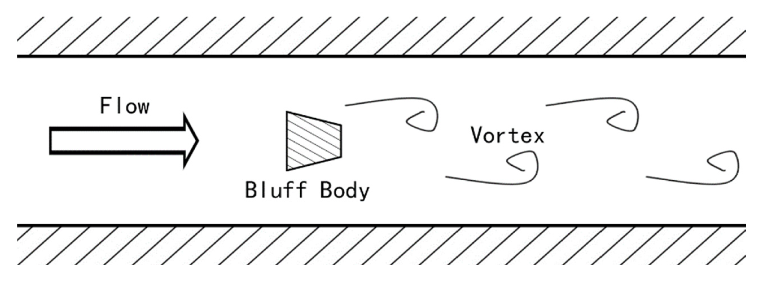
2.1.1. Principle of Karman Vortex

Figure 1 shows the cross-section of the vortex flowmeter. Under specific flow conditions, when the fluid medium passes through the bluff body, regular vortices alternately form behind it, which is a phenomenon known as the Karman vortex street. The development of vortex flowmeters is fundamentally based on this Karman vortex street phenomenon, with the relationship between the frequency f generated by the vortex street and the flow rate U being expressed as Equation (1):

$$f=St{\displaystyle \frac{U_1}{d}}=St{\displaystyle \frac{U}{md}}$$

(1)

where f is the frequency of vortex generation (Hz), St is the Strouhal number (dimensionless), U₁ is the average flow rate of the fluid on both sides of the vortex bluff body (m/s), d is the width of the onstream surface of the vortex bluff body (m), U is the average flow velocity in the pipeline (m/s), and m is the ratio of the area of the fluid area in the section where the intake surface of the vortex generating body is located to the cross-sectional area of the pipeline.

Equation (2) shows the definition of m in Equation (1):

$$m=1-{\displaystyle \frac{2}{\pi }}\left[{\displaystyle \frac{d}{D}}\sqrt{1-{\left({\displaystyle \frac{d}{D}}\right)}^2}+\arcsin {\displaystyle \frac{d}{D}}\right]$$

(2)

In the formula, D represents the inner diameter of the pipeline, and d is the characteristic length of the bluff body. In addition, d/D is also the blocking ratio.

The flow rate inside the pipeline is

$$Q={\displaystyle \frac{\pi U{D}^2}{4}}={\displaystyle \frac{\pi D^{2}mdf}{4St}}={\displaystyle \frac{f}{K}}$$

(3)

In Equation (3), K represents the K coefficient, which equals 1/L.

Under the influence of a specific shape of the bluff body, the frequency of the bluff body is proportional to the flow velocity of the fluid. The bluff body is perpendicular to the flow direction, and the detection element placed at the wake of the bluff body applies the received lift in the form of stress to the piezoelectric crystal element, converting it into an alternating charge signal. After charge amplification, filtering, and shaping, the vortex frequency signal is obtained, and the flow rate of the fluid can be measured by conversion.

The regular alternation of vortices behind the bluff body is influenced by the symmetry of its geometric configuration. Symmetrical bluff bodies tend to produce more stable and predictable vortex shedding patterns, which are crucial for accurate flow measurement.

In previous studies, the operating range of vortex flowmeters was kept as low as possible to ensure Re < 20,000. When Re > 20,000, the nonlinearity of the Strouhal number is an inherent characteristic of vortex shedding.

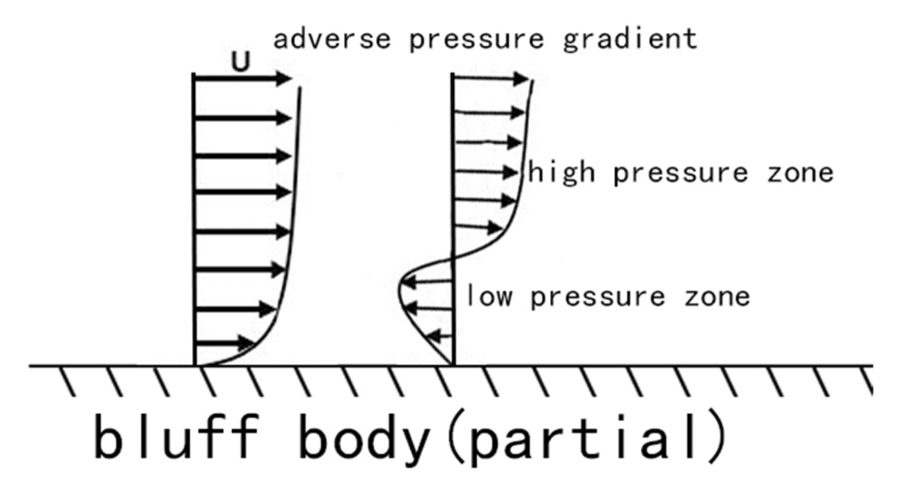
2.1.2. Boundary Layer Theory

The boundary layer is a thin layer of flow in high Reynolds number flow where the viscous force closely adheres to the object’s surface and cannot be ignored. For fluids with small viscosity, all frictional losses occur within the boundary layer, while the flow outside the boundary layer can be considered as frictionless flow. The flow field of micro-viscous fluids is divided into two regions: the boundary layer and the outflow region. In the boundary layer, the velocity gradient along the normal direction of the wall is significant, and the wall has an undeniable impact on the fluid flow. The velocity gradient along the normal wall in the outflow zone is very small and can be considered an ideal fluid. When the flow area of the fluid expands, the velocity slows down, and there is a reverse pressure zone, boundary layer separation phenomenon will occur, as shown in Figure 2, which is the main reason for the formation of the Karman vortex Street phenomenon. For vortex flowmeters, when the flow velocity is too low, the boundary layer separates earlier, but due to insufficient momentum to maintain the stability of the vortex, it cannot be sensed by the sensor. When the flow velocity is too high, the boundary layer separates later, the vortex column distance is too close, the vortex street is not stable enough, and the signal-to-noise ratio will deteriorate [35].

2.1.3. Navier–Stokes Equations

The Navier–Stokes equations, derived from Newton’s second law, describe the conservation of momentum in fluid motion. Their general form is as follows:

$$\rho ({\displaystyle \frac{\partial u}{\partial t}}+u\cdot \nabla u)=-\nabla p+\mu {\nabla }^{2}u+f$$

(4)

where

ρ is the fluid density, representing the mass per unit volume of the fluid;

u is the velocity vector, representing the speed of fluid motion in space;

p is the pressure, representing the internal pressure of the fluid;

μ is the dynamic viscosity, representing the internal friction characteristics of the fluid;

f is the body force, such as gravity or centrifugal force, representing the external forces acting on the fluid.

In addition, the term ∇u in the equation represents the divergence of the velocity vector, used to describe the compressibility of the fluid. In this research, it equals 0, meaning the fluid is incompressible.

2.1.4. Reynolds-Averaged Navier–Stokes (RANS) Equations

The Navier–Stokes equations are among the most fundamental equations in fluid mechanics, widely used to describe various fluid flow phenomena, including both laminar and turbulent flows. However, due to their nonlinearity and complexity, directly solving the Navier–Stokes equations is often very challenging, especially in high Reynolds number turbulent flows. Therefore, turbulence models are usually introduced to simplify the solution process. In this study, we employed the Reynolds-Averaged Navier–Stokes (RANS) equations combined with the RNG k-ε turbulence model to simulate the flow phenomena in vortex flowmeters. These equations are derived by decomposing the velocity and pressure fields into mean (averaged) and fluctuating (turbulent) components:

$$\begin{array}{l}u=\overline{u}+u\prime \\ p=\overline{p}+p\prime \end{array}$$

(5)

where u and p are the mean velocity and pressure, while u′ and p′ represent the turbulent fluctuations. Substituting these decompositions into the Navier–Stokes equations and averaging over time or space, we obtain the RANS equations:

$$\rho ({\displaystyle \frac{\partial u}{\partial t}}+\overline{u}\cdot \nabla \overline{u})=-\nabla \overline{p}+\mu {\nabla }^2\overline{u}-\nabla \cdot \overline{u\prime u\prime }$$

(6)

Here, the term $\nabla \cdot \overline{u\prime u\prime }$ represents the Reynolds stress tensor, which accounts for the effects of turbulent fluctuations on the mean flow. This term must be modeled to close the RANS equations.

2.1.5. RNG k-ε Model

Turbulence is a very common flow phenomenon, and the vast majority of natural flows are turbulent. Reynolds Average Navier–Stokes (RANS) establishes a model by statistically averaging the mass, momentum, and energy transport equations of the flow. It does not require the calculation of turbulence fluctuations at various scales, only the average motion, so the computational workload is small. In this study, the RNG k-ε model under RANS was chosen, which has high accuracy and wide applications. Like vortex flowmeters, it requires high Reynolds numbers.

In the RNG k-ε model, $\nabla \cdot \overline{u\prime u\prime }$ in the RANS equations is modeled using the turbulent viscosity μ_t and turbulent kinetic energy k:

$$\overline{u\prime u\prime }={\displaystyle \frac{2}{3}}kI-{\mu }_t(\nabla \overline{u}+{(\nabla \overline{u})}^T)$$

(7)

where

I is the identity tensor; $\nabla u$ is the mean strain rate tensor; ${(\nabla u)}^T$ is its transpose.

Here is the transport equation for Turbulent Kinetic Energy k:

$${\displaystyle \frac{\partial }{\partial t}}(\rho k)+{\displaystyle \frac{\partial }{\partial x_i}}(\rho u_{i}k)={\displaystyle \frac{\partial }{\partial t}}\left[(\mu +{\displaystyle \frac{{\mu }_t}{{\sigma }_k}}){\displaystyle \frac{\partial k}{\partial x_j}}\right]+G_k+G_b-\rho \epsilon +S_k$$

(8)

where

ρ is the fluid density.

u_i is the mean velocity.

μ is the molecular viscosity.

μ_t is the turbulent viscosity.

σ_k is the turbulent Prandtl number for the k equation, which is 1.0.

G_k is the generation term of turbulent kinetic energy by mean velocity gradients.

G_b is the generation term of turbulent kinetic energy by buoyancy.

ε is the dissipation rate of turbulent kinetic energy.

S_k is the user-defined source term.

$${\displaystyle \frac{\partial }{\partial t}}(\rho \epsilon )+{\displaystyle \frac{\partial }{\partial x_i}}(\rho u_i\epsilon )={\displaystyle \frac{\partial }{\partial x_j}}\left[(\mu +{\displaystyle \frac{{\mu }_t}{{\sigma }_{\epsilon }}}){\displaystyle \frac{\partial \epsilon }{\partial x_j}}\right]+C_{1\epsilon }{\displaystyle \frac{\epsilon }{k}}{G}_k+C_{2\epsilon }{\displaystyle \frac{\epsilon }{k}}{G}_b-C_{3\epsilon }\rho {\displaystyle \frac{{\epsilon }^2}{k}}+S_{\epsilon }$$

(9)

where

σ_ε is the turbulent Prandtl number for the ϵ equation, which is 1.3.

S_ε is the user-defined source term.

C_1ε, C_2ε, and C_3ε are model constants, with typical values of 1.44, 1.92, and 0.09, respectively.

The RNG k-ε model introduces a special term R_ε in the ε equation to enhance the response to rapid strain and streamline curvature:

$$R_{\epsilon }={\displaystyle \frac{C_{3\epsilon }\rho {\epsilon }^2}{k}}(1-{\displaystyle \frac{k^{3/2}}{\epsilon L}})$$

(10)

where L is the integral length scale.

Here are the assumptions in this model:

Reynolds Averaging Assumption: The model is based on the RANS equations, which involve decomposing instantaneous flow variables into mean and fluctuating components. This process eliminates the turbulent structures from the flow, resulting in equations for the mean velocity and pressure fields.

Eddy Viscosity Assumption: The eddy viscosity (turbulent viscosity) is introduced to relate the Reynolds stresses to the mean velocity gradients. This assumption simplifies the closure problem by expressing the turbulent stresses in terms of a single scalar quantity, the eddy viscosity.

Boussinesq Assumption: The Reynolds stress is proportional to the mean strain rate tensor.

2.1.6. Lift Coefficient and Drag Coefficient

The lift (drag) coefficient is a dimensionless parameter that quantifies the lift(drag) force generated by an object moving through a fluid. They could be defined by the equation below:

$$\begin{array}{l}{C}_L={\displaystyle \frac{L}{{\displaystyle \frac{1}{2}}\rho v^{2}S}}\\ C_D={\displaystyle \frac{D}{{\displaystyle \frac{1}{2}}\rho v^{2}S}}\end{array}$$

(11)

where

L is the lift force, and D is the drag force. ρ is the fluid density. V is the velocity of the object relative to the fluid. S is the reference area.

2.2. Geometric Modeling and Meshing

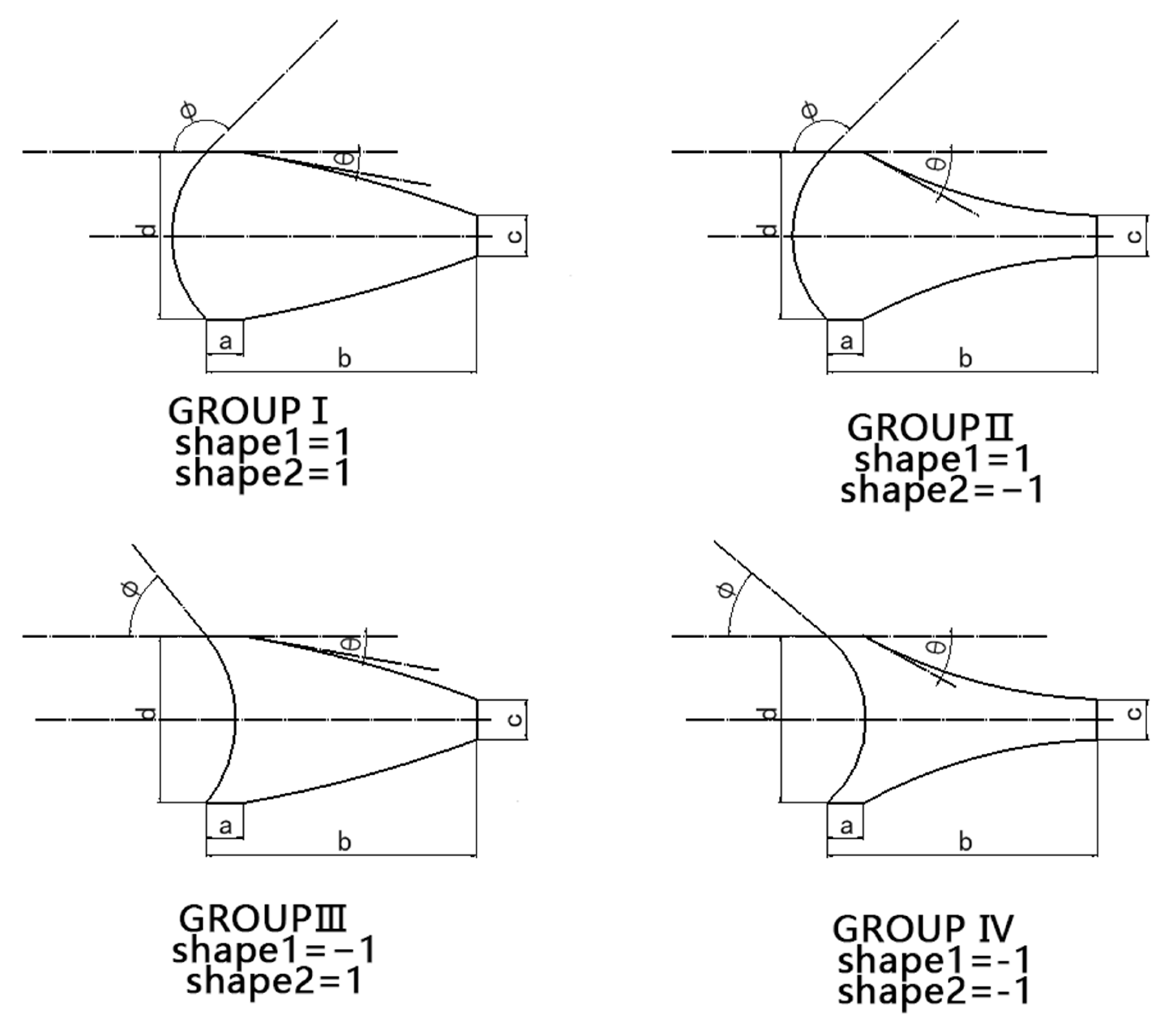
2.2.1. Definition of Dimension Parameters

The trapezoidal bluff body is extensively utilized in vortex flowmeters due to its significant two-dimensional vortex flow characteristics under unsteady turbulent conditions [10]. To further investigate the impact of curved edges on the performance of bluff bodies, this study employs arcs instead of straight lines to derive four novel bluff body shapes from the trapezoidal bluff body, examining their vortex characteristics under varying geometric parameters.

As shown in Figure 3, four shapes are defined according to the concavity of the 2 arcs, which are positive–positive (top left), positive-negative (top right), negative–positive (bottom left), and negative–negative (bottom right).

The input parameters of the model are as follows:

a	transition edge, parallel to the direction of flow velocity, located between the forward arc and backward arc. Structural parameter
b	bluff body length, parallel to the direction of flow velocity, equals the length of a bluff body projected parrel to the direction of flow velocity. Structural parameter
c	downstream width, vertical to the direction of flow velocity, equals the minimum distance between two backward arcs. Structural parameter
d	upstream width, vertical to the direction of flow velocity, equals the width of a bluff body projected perpendicular to the direction of flow velocity. It determines the blockage ratio of a bluff body. It is also the characteristic length. Structural parameter
ϕ	the angle between the horizontal direction and the tangent at the intersection point of the forward arc with a (transition edge). Structural parameter
θ	the angle between the horizontal direction and the tangent at the intersection point of the backward arc with a (transition edge). Structural parameter
Shape1	defined by the shape of the forward arc. When the arc is convex (positive), the value is 1; when the arc is concave (negative), the value is −1. Shape parameter
Shape2	defined by the shape of the backward arc. When the arc is convex (positive), the value is 1; when the arc is concave (negative), the value is −1. Shape parameter

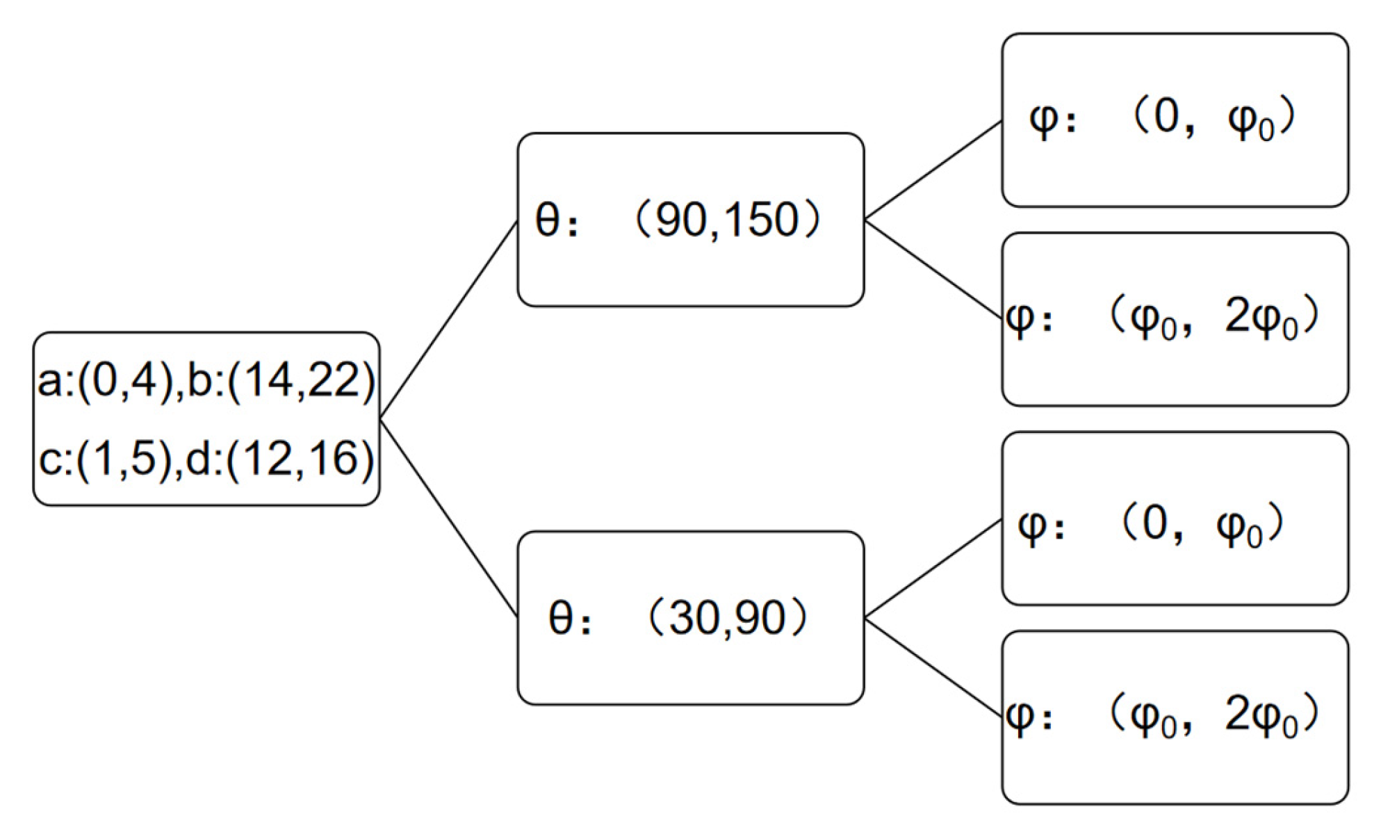
2.2.2. Latin Hypercube Sampling Method

Latin Hypercube Sampling (LHS) was proposed by Mckay et al. in 1979 [36]. This method is a stratified sampling technique. By dividing the range of each input variable into equal-length intervals of equal probability, each sample point is randomly selected within each interval, and then these sample points are combined into a sample vector, ensuring the uniform distribution of samples in the multidimensional space. This ensures a uniform distribution of big data samples, which is beneficial for subsequent analysis.

As shown in Figure 4, firstly, the four parameters a, b, c, and d take random values within their designated intervals. Then, the interval of θ is selected according to the value of shape1: when shape1 = −1, θ is located at (30°, 90°); when shape1 = 1, θ is at (90°, 150°). Finally, the interval of φ is chosen based on the value of shape2: when shape2 = −1, φ is located at (φ₀, 2φ₀); when shape2 = 1, φ is located at (0, φ₀). Eventually, 2500 bluff bodies of different sizes are generated for each shape, totaling 10,000 bluff bodies.

The interval range of θ and φ is set to consider the shape of the bluff body: if the radius of the planes is too small, the shape of the bluff body will be significantly distorted, severely deviating from the ideal trapezoidal form, which cannot be classified to straight-edged bluff body derived shape.

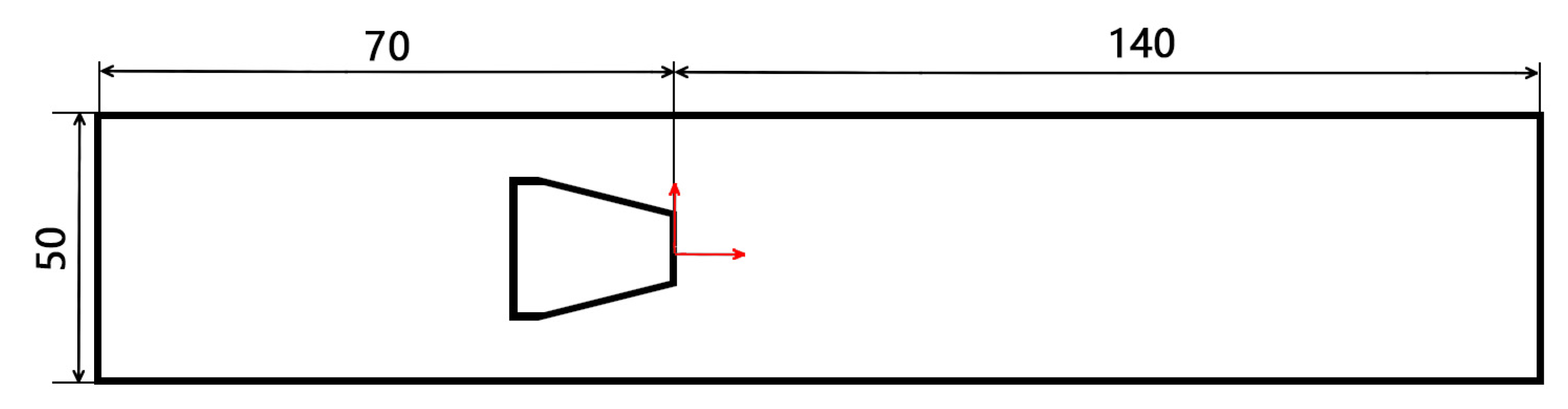
2.2.3. Flow Field Modeling

Based on Ansys Design Modeler, a two-dimensional vortex flowmeter section model of a DN50 pipeline is established. The flow channel size and coordinate origin are shown in Figure 5.

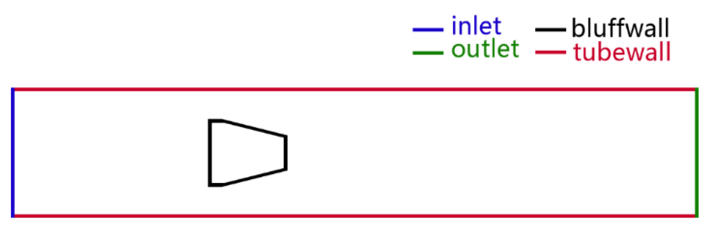
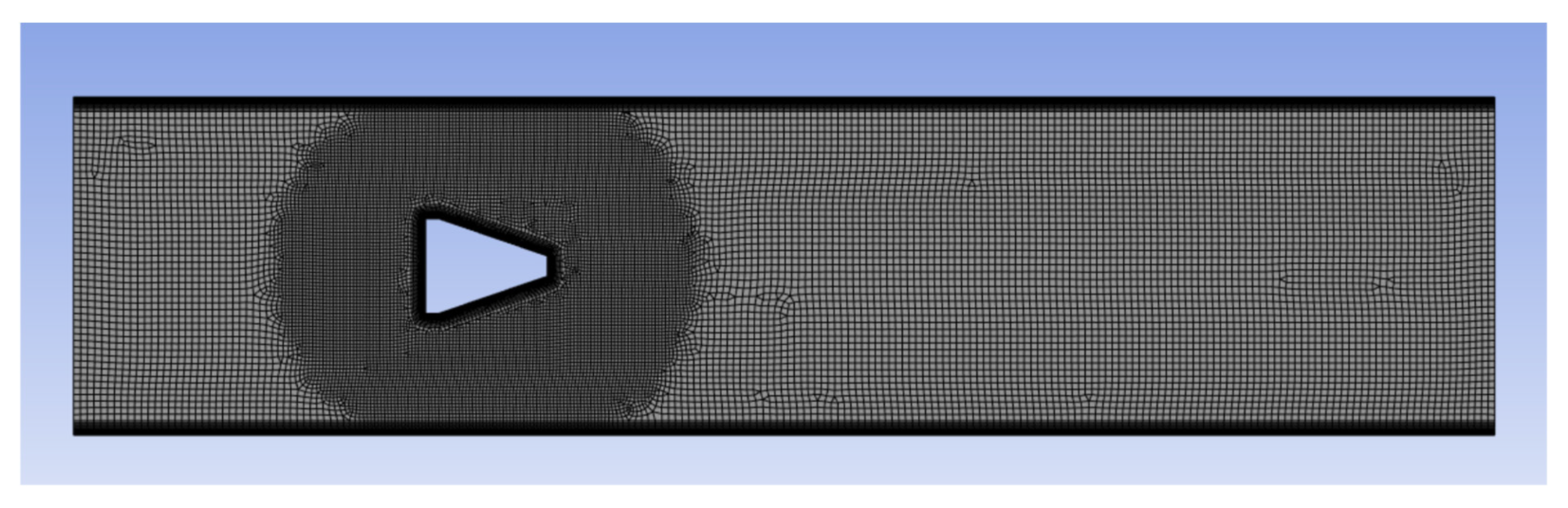
2.2.4. Mesh Division and Naming Selection

ANSYS Meshing software was utilized for grid division. The naming selection is shown in Figure 6: the bluff body is set to bluffwall, and the pipe wall is set to tubewall. The fluid inlet is set to inlet and the pressure outlet to outlet.

The following shows the options of meshing:

Mesh type	Quad/Tri
Global mesh	1 mm
Refined mesh	0.5 mm, Circle, the radius of the refined area is 30 mm, and its center coordinate is (−9, 0, 0).
Expansion	On bluffwall and tubewall, the thickness of the first layer is 0.1 mm, the number of layers was 12, and the growth rate was 1.1.

Taking the straight-edge bluff body as an example, with a = 2, b = 18, c = 3, and d = 14, there are 23,782 nodes and 23,454 elements after the division is complete. Figure 7 shows the detail of the mesh grid.

2.3. Build the Simulation Model

2.3.1. Serial Simulation Technology

In actual simulations, most of the computing time is consumed before the vortex street stabilizes. However, when a structure that generates a stable vortex street transformation is modified, the required computational time is significantly reduced. Therefore, serial simulation techniques are especially useful. Specifically, the 10,000 bluff bodies are divided into 2500 design points according to one of the four shapes in each group to form a sampling group. To ensure that the first design point in the sampling group can reach a stable state, two design points are set in front of the sampling group as a stabilizing group. When the two adjacent design points are identical, Ansys will skip duplicate design points; thus, the size parameters of the stabilizing group (dp1 and dp0) need to be slightly different.

Separate simulations and serial simulations are performed on the linear bluff body during grid division, as shown in Figure 8. The green lines represent two stabilizing design points and one simulation design point, with different lines used for distinction.

Figure 8 illustrates the relationship between the difference in two peaks and time. As shown in Figure 8, when the simulation is conducted separately, V14 requires approximately 400 steps to reach stability. When serial simulation is employed, the vortex street reaches a stable state within a short time after switching design points. Serial simulation effectively reduces the simulation time. Through serial simulation technology, time steps can be reduced from 1000 to 500, saving 50% of costs. Also, the maximum velocity becomes constant after more steps; conducting more steps of simulation is not very effective.

Figure 8 shows that for each design point, it needs less than 200 steps to reach the stable state. Figure 9 shows the residuals during CFD simulation. In CFD simulations, residuals are used to measure the difference between the computed results and the exact solution. As the number of iterations increases, the residuals gradually stabilize, indicating that the simulation results are converging. Figure 9 shows the variation in residuals during the simulation process. It can be seen that after 200 time steps (i.e., 8000 iterations), the residuals gradually stabilize, which indicates that the simulation results have converged. To ensure accuracy, the data from the first 200 steps were discarded.

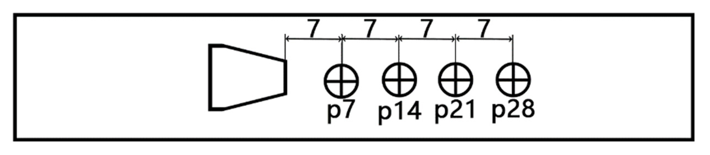
2.3.2. Monitored Parameters Setting

As shown in Figure 10, on the centerline of the flow channel, a velocity monitoring point is set every 0.5d (7 mm) downstream of the generating body, used to monitor the velocity in the y-direction. A total of four monitoring points are established, named p7, p14, p21, and p28.

The monitored parameters of the model are as follows:

p7	The velocity in the y-direction of p7
p14	The velocity in the y-direction of p14. In industrial production, the probe is often located at here
p21	The velocity in the y-direction of p21
p28	The velocity in the y-direction of p28
Pin	The average pressure of fluid inlet
Pout	The average pressure of fluid outlet
CL	bluff body wall (bluffwall) lift coefficient
CD	bluff body wall (bluffwall)drag coefficient

As shown in Figure 9, on the centerline of the flow channel, a velocity monitoring point is set every 0.5d (7 mm) downstream of the generating body, used to monitor the velocity in the y-direction. A total of four monitoring points are established, named p7, p14, p21, and p28. Simultaneously, pressure monitoring points are set at the inlet (Inlet) and outlet (Outlet) of the flow channel to monitor the inlet pressure (P_in) and outlet pressure (P_out). Additionally, the lift coefficient (C_l) and drag coefficient (C_d) are monitored on the surface of the bluff body wall.

2.3.3. CFD Parameter Setting

The selection of CFD parameters is based on the choices made in previous studies [8,9,37]. The settings are below:

Fluid type	air
Design points	2500 in total
Shapes	4 shapes per design point
Model	RNG k-ε
Time step	0.0005 s, 500 steps(per design point)
Iteration number	20 times/step
Inlet	5 m/s
Bluffwall and Tubewall	no-slip boundary conditions
Outlet	gauge pressure 0 Pa

2.3.4. Mesh Simulation Verification

Simulating the straight-edge bluff body used in grid division, the results are shown in

Table 1. Mesh independence verification.

Cells	12,073	20,893	23,454	25,379	28,107
$\overline{V}$	4.86033	4.88430	4.90668	4.98842	5.00682
err	−2.93%	−2.45%	−2.00%	−0.37%	--

, where the average values of V₇, V₁₄, V₂₁, and V₂₈ are obtained. The error of the table density used in the simulation is 2%. For this dataset, the accuracy is sufficient, and increasing the accuracy would significantly increase the total simulation time of the dataset.

2.4. Mathematics Method

2.4.1. Fast Fourier Transform

In the field of signal processing, the computation of Discrete Fourier Transform (DFT) occupies a crucial position. Whether it is signal correlation analysis, filtering processing, or spectral estimation, they all rely on the support of DFT [38].

The continuous Fourier transform of discrete-time signal x (n) is defined as follows:

$$X\left(e^{j\omega }\right)={\displaystyle \sum _{k=0}^{N-1}x(n)e^{j\omega }}$$

(12)

To obtain an N-point DFT, N² complex multiplication operations and N (N − 1) complex addition operations are required. When the value of N becomes very large, the computational workload will become quite large, which may lead to issues with computational efficiency.

The FFT algorithm reduces the computational complexity of DFT from O (N²) to O (NlogN) through a divide-and-conquer strategy, significantly improving computational efficiency. When discussing mathematical transformations of curves, they can be viewed as functions with two variables x and y. Quoting the Fourier transform of a two-dimensional continuous function, let f (x, y) be a function of two independent variables x, y, When they satisfy ${\displaystyle {\int }_{-\infty }^{\infty }{\displaystyle {\int }_{-\infty }^{\infty }\left|f(x,y)\right|dxdy<0}}$, FFT definition formula is shown in Equation (5):

$$F(u,v)={\displaystyle {\int }_{-\infty }^{\infty }{\displaystyle {\int }_{-\infty }^{\infty }f(x,y)e^{-j2\pi (ux+uy)}dxdy}}$$

(13)

FFT is an efficient algorithm widely used in signal processing, image processing, communication systems, and other fields. It significantly reduces the computational complexity of DFT through a divide-and-conquer strategy, making large-scale signal processing possible. FFT not only holds significant importance in theoretical research but also plays a crucial role in practical applications. In this article, FFT is used to solve the frequency of velocity.

2.4.2. Grey Relation Analysis

Grey Relation Analysis (GRA) is a method used for multi-factor statistical analysis, primarily employed to address problems in gray systems with incomplete information and small data volumes. The input parameters are taken as the comparison sequence, and the output parameters as the reference sequence:

$$\xi (x_i(k))={\displaystyle \frac{{∆}_{\min }+\rho {∆}_{\max }}{\left|{∆}_{oi}(k)\right|+\rho {∆}_{\max }}}$$

(14)

where Δ_min is the minimum difference between the two levels, Δ_max is the maximum difference between the two stages, Δ_0i(k) is the absolute difference between the reference sequence and the comparison sequence at the k-th moment, ρ is the resolution coefficient (usually 0.5), and the correlation coefficient is the average of the correlation coefficients, indicating the overall similarity of the comparison sequence to the reference sequence. The formula to calculate r_i is

$$r_i={\displaystyle \frac{1}{n}}{\displaystyle \sum _{k=1}^n\xi (x_i(k))}$$

(15)

Grey relational grade r is a value from 0 to 1, which reflects the extent of the relation between the comparison sequence x_i(k) and reference one x₀(k). In this paper, output parameters are comparison sequences and input parameters are reference sequences. Particularly, if two sequences are identical, then grey relational grade is equal to 1.

2.4.3. Kernel Ridge Regression

Kernel Ridge Regression (KRR) is a machine learning algorithm that combines Ridge Regression with kernel methods [39,40]. It can be considered as Support Vector Regression (SVR), which employs ε insensitive quadratic loss and sets ε to 0 [41]. It leverages the kernel trick to map data into a high-dimensional space and then applies Ridge Regression in that space, enabling the handling of nonlinear relationships. KRR excels at dealing with complex nonlinear data while maintaining the regularization properties of Ridge Regression to prevent overfitting.

The advantage of KRR is that its optimization problems can be efficiently solved through analytical solutions, which makes it perform well on medium-sized datasets. In addition, KRR’s model is non-sparse, meaning that all training data points contribute to the model, making it more stable during prediction [42].

Generally, the expression for the RBF kernel function is

$$K(x,y)=\exp (-\gamma {‖x-y‖}^2)$$

(16)

where

x and y are input data points.

$‖x-y‖$ is the Euclidean distance between x and y.

γ is the parameter of the RBF kernel, controlling the width of the Gaussian kernel. When γ is large, the similarity between data points decreases more rapidly. When γ is small, the similarity between data points decreases more slowly.

In KRR, the kernel matrix K(x,y) is symmetric, which ensures that the relationships between input parameters are consistently captured. This symmetry is crucial for the stability and generalization of the model. The symmetric nature of the kernel matrix helps in accurately mapping the input parameters to the output performance indicators, thereby improving the predictive accuracy of the model.

For Kernel Ridge Regression, the objective is to minimize the following loss function:

$$L(w)={{\displaystyle \sum _{i=1}^n{(y_i-w^T\varphi (x_i))}^2+\alpha ‖w‖}}^2$$

(17)

where

y_i is the target value.

ϕ(x_i) is the feature vector after mapping through the kernel function.

w is the regression coefficient vector.

α is the regularization parameter. Larger α leads to underfitting, and smaller α leads to overfitting.

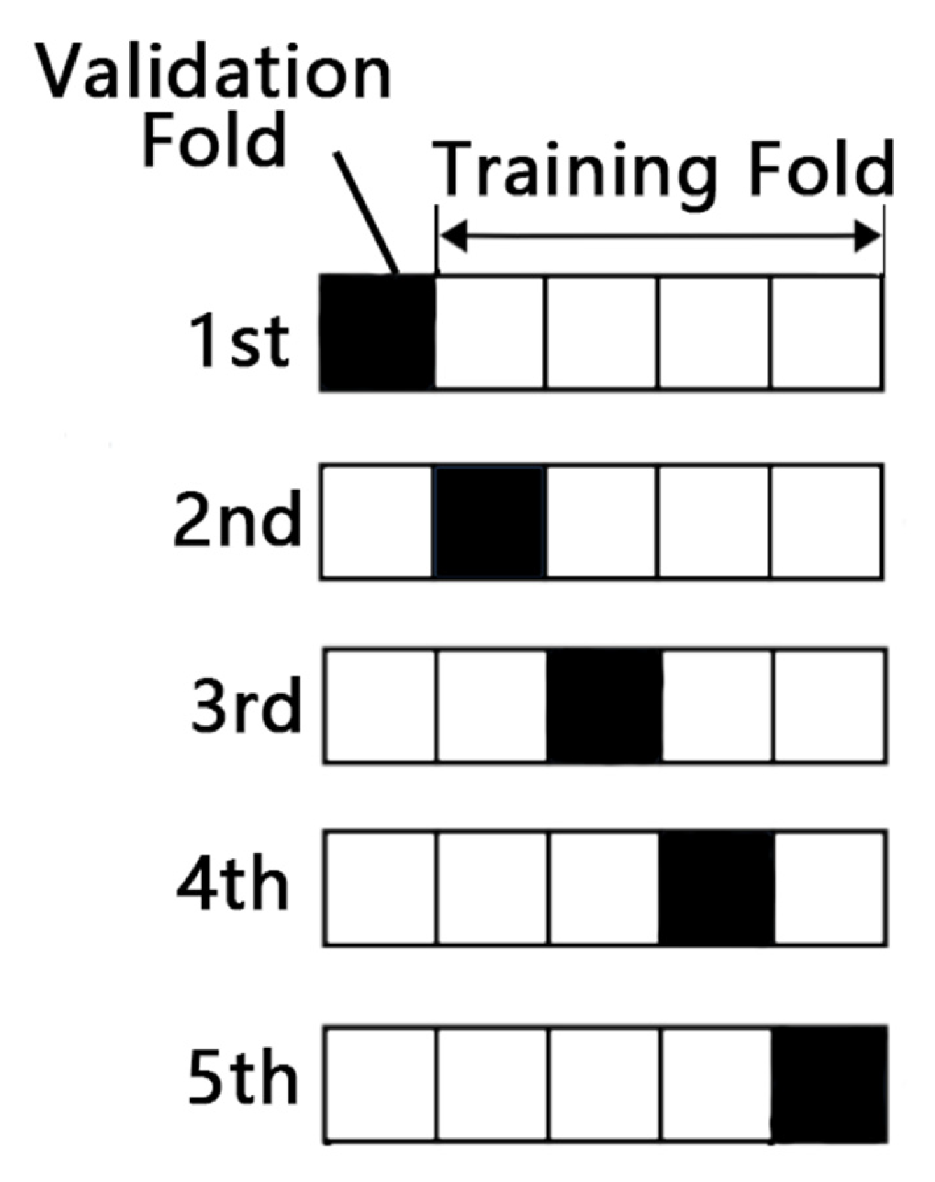
2.4.4. K-Fold Cross-Validation

K-fold cross-validation is a statistical analysis method used for model evaluation and selection. It involves dividing the dataset into K mutually exclusive subsets of approximately equal size (referred to as “folds”) to ensure that the model has good generalization capability during training and testing. This method effectively utilizes limited data and reduces the risk of model overfitting [43].

As shown in Figure 11, in K-Fold Cross-Validation, each subset is used as the validation fold once during the validation process, while the remaining subsets are combined to form the training fold. The average of the trained models is ultimately used as the final prediction result.

2.5. Evaluation Criteria

MSE (Mean Squared Error) is the average of the squares of the differences between the predicted values and the actual values. It reflects the degree of discrepancy between the predicted and actual values. It is defined by Equation (18):

$$MSE={\displaystyle \frac{1}{n}}{\displaystyle \sum _{i=1}^n{(y_i-{\widehat{y}}_i)}^2}$$

(18)

where y_i represents the actual value, $\widehat{y_i}$ represents the predicted value, and n is the number of samples.

RMSE (Root Mean Squared Error) is the square root of MSE. It represents the sample standard deviation of the differences between the predicted and actual values. It is defined by Equation (19):

$$RMSE=\sqrt{MSE}=\sqrt{{\displaystyle \frac{1}{n}}{\displaystyle \sum _{i=1}^n{(y_i-{\widehat{y}}_i)}^2}}$$

(19)

MAE (Mean Absolute Error) is the average of the absolute differences between the predicted and actual values. It directly reflects the average level of prediction errors. It is defined by Equation (20):

$$MAE={\displaystyle \frac{1}{n}}{\displaystyle \sum _{i=1}^n\left|y_i-{\widehat{y}}_i\right|}$$

(20)

R² (Coefficient of Determination) is used to measure the proportion of the variance of the dependent variable that is explained by the model. It is defined by Equation (21):

$$R^2=1-{\displaystyle \frac{{\displaystyle \sum _{i=1}^n{(y_i-{\widehat{y}}_i)}^2}}{{\displaystyle \sum _{i=1}^n{(y_i-\overline{y})}^2}}}$$

(21)

where $\overline{y}$ is the mean of the actual values. R² value ranges from 0 to 1. The closer it is to 1, the stronger the model’s ability to explain the data.

In the evaluation of this fit, MSE, RMSE, and MAE are employed to assess the correlation. Meanwhile, the variance and mean of the RMSE from the results of K-fold cross-validation are utilized to evaluate the uncertainty.

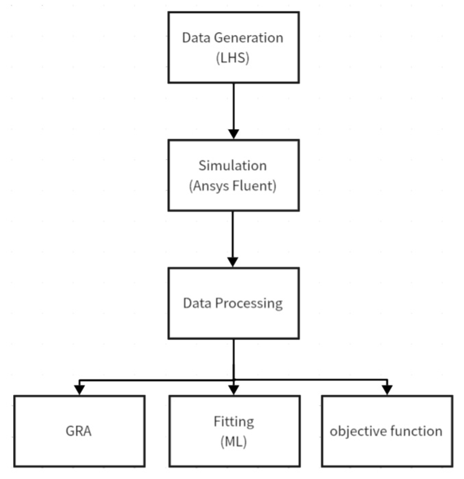
2.6. Research Process

2.6.1. Main Research Process

Figure 12 shows how this research was conducted. In this study, the input parameters were first generated using the LHS method by importing Python code into Ansys Fluent. Then, preprocess the data generated by Ansys 2023R1 Fluent simulation using Python. The preprocessed data are applied in ML, GRA, and objective function analysis.

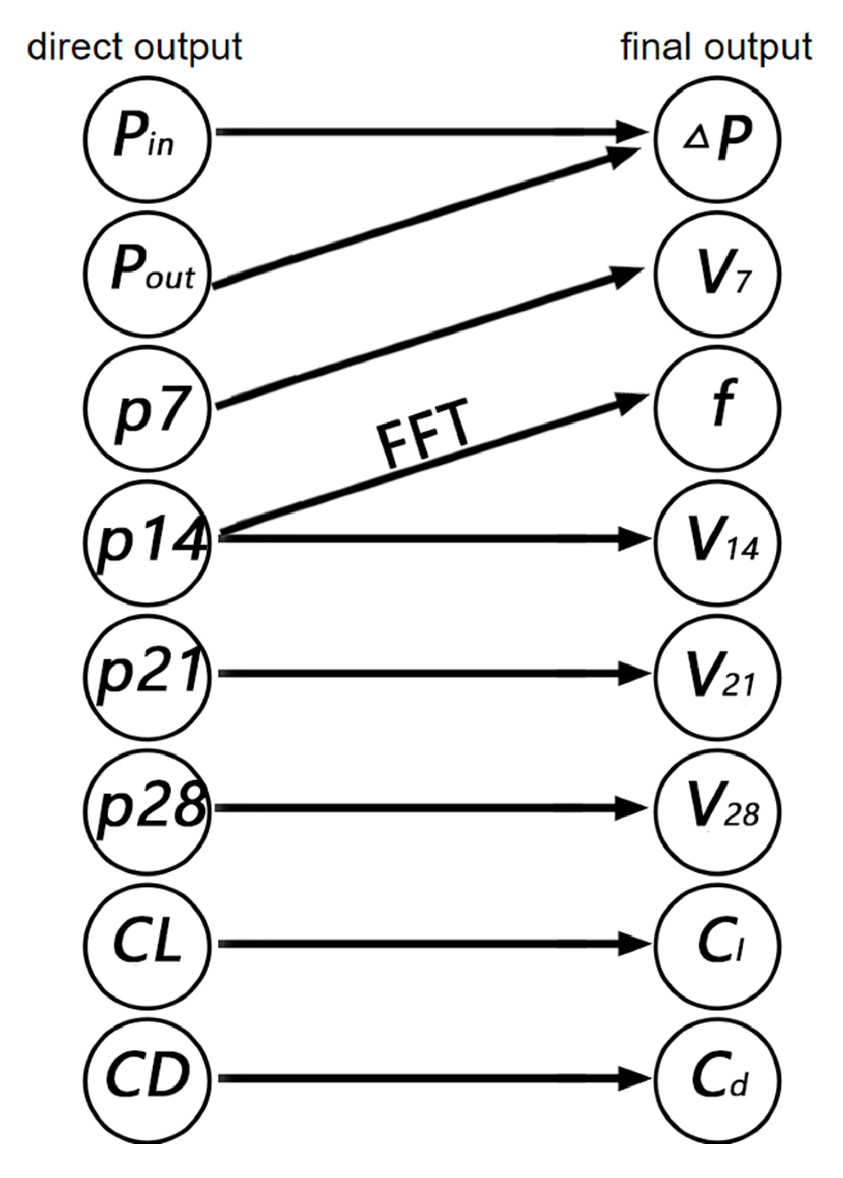
2.6.2. Preliminary Data Processing

As shown in Figure 13, for the subsequent 300-step data, conduct the data process below:

V7	Average peak value of envelope curve of y-direction velocity–time curve at p7
V14	Average peak value of envelope curve of y-direction velocity–time curve at p14, which shows the strength of probe signal
V21	Average peak value of envelope curve of y-direction velocity–time curve at p21
V28	Average peak value of envelope curve of y-direction velocity–time curve at p28
ΔP	The difference between Pin and Pout, represents the pressure loss of the system
f	The result of FFT of y-direction velocity–time curve at p7 (probe), showing the frequency of velocity
Cl	Average peak value of envelope curve of lift coefficient-time curve at p7
Cd	Average peak value of envelope curve of drag coefficient-time curve at p7

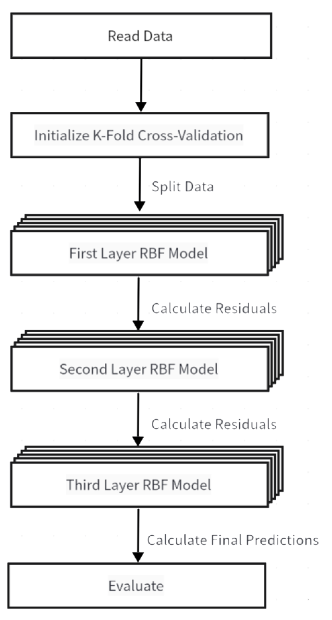
2.6.3. Fitting Modeling Principles

In this study, a regression iterative model was established based on RBF kernel function classes of the scikit-learn machine learning library in Python 3.12.

In the field of deep learning, Residual Learning’s core idea is to introduce residual modules that directly pass the input signal to subsequent layers through skip connections while allowing the network to learn the residual between the input and output. This paper draws on this idea, approximating the target value step by step through layer-by-layer residual fitting. Compared with traditional residual learning, it focuses more on improving the prediction accuracy of regression models through multi-stage residual fitting. This paper employs a three-layer fitting method, all utilizing the RBF kernel function.

As shown in Figure 14, the first layer of KRR fits the relationship between input parameters and output parameters. The second and third layers fit the relationship between the residuals from the previous layer and the input parameters. To avoid overfitting, K-fold cross-validation is employed, dividing the data into five folds and randomly shuffling the data before splitting. The final prediction model is based on the average of the predictions obtained from each training iteration.

2.6.4. KRR Parameter Validation

In KRR, the parameters α and γ are crucial, directly affecting the fitting accuracy and outcomes. Utilizing grid search cross-validation, the RMSE of V₇, V₁₄, V₂₁, and V₂₈ is calculated to identify the optimal parameters for each of the three KRRs.

Among them, the parameter analysis for the first layer was conducted first, and the residuals from the best-performing group were utilized for the second layer analysis. The third layer followed a similar approach. As indicated by

Table 2. Mean squared error table of first layer.

α\γ	0.001	0.01	0.1	1	10
0.001	2.252984	3.257195	4.573021	15.77358	17.213374
0.01	2.226058	2.663419	4.309725	15.78435	17.213387
0.1	2.208787	2.383252	3.566977	15.8839	17.213505
1	2.241499	2.283818	3.180383	16.4318	17.214113
10	2.340610	2.343677	5.973044	17.062324	17.214735

, the optimal parameters for the first layer are α = 0.1 and γ = 0.001;

Table 3. Mean squared error table of second layer.

α\γ	0.001	0.01	0.1	1	10
0.001	2.154387	3.057694	4.165838	2.090351	2.074577
0.01	2.119666	2.498945	3.863205	2.090066	2.074577
0.1	2.098079	2.263090	2.999811	2.087597	2.074579
1	2.085735	2.149949	2.301291	2.078392	2.074594
10	2.079093	2.097154	2.093280	2.074679	2.074609

reveals that the best parameters for the second layer are α = 0.001 and γ = 10; and

Table 4. Mean squared error table of third layer (×10⁻⁶).

α\γ	0.001	0.01	0.1	1	10
0.001	2.150070	3.051704	4.158544	2.086428	2.070426
0.01	2.115421	2.494018	3.856163	2.086142	2.070426
0.1	2.093876	2.258582	2.994172	2.083657	2.070427
1	2.081551	2.145628	2.296846	2.074360	2.070434
10	2.074920	2.092930	2.089104	2.070538	2.070443

shows that the optimal parameters for the third layer are α = 0.001 and γ = 10. In the third layer, there was a significant reduction in the order of magnitude of the residuals. Given that the simulation accuracy of Ansys is at 10⁻⁶, proceeding to a fourth layer would be almost meaningless and could potentially increase the risk of overfitting.

3. Data Analysis

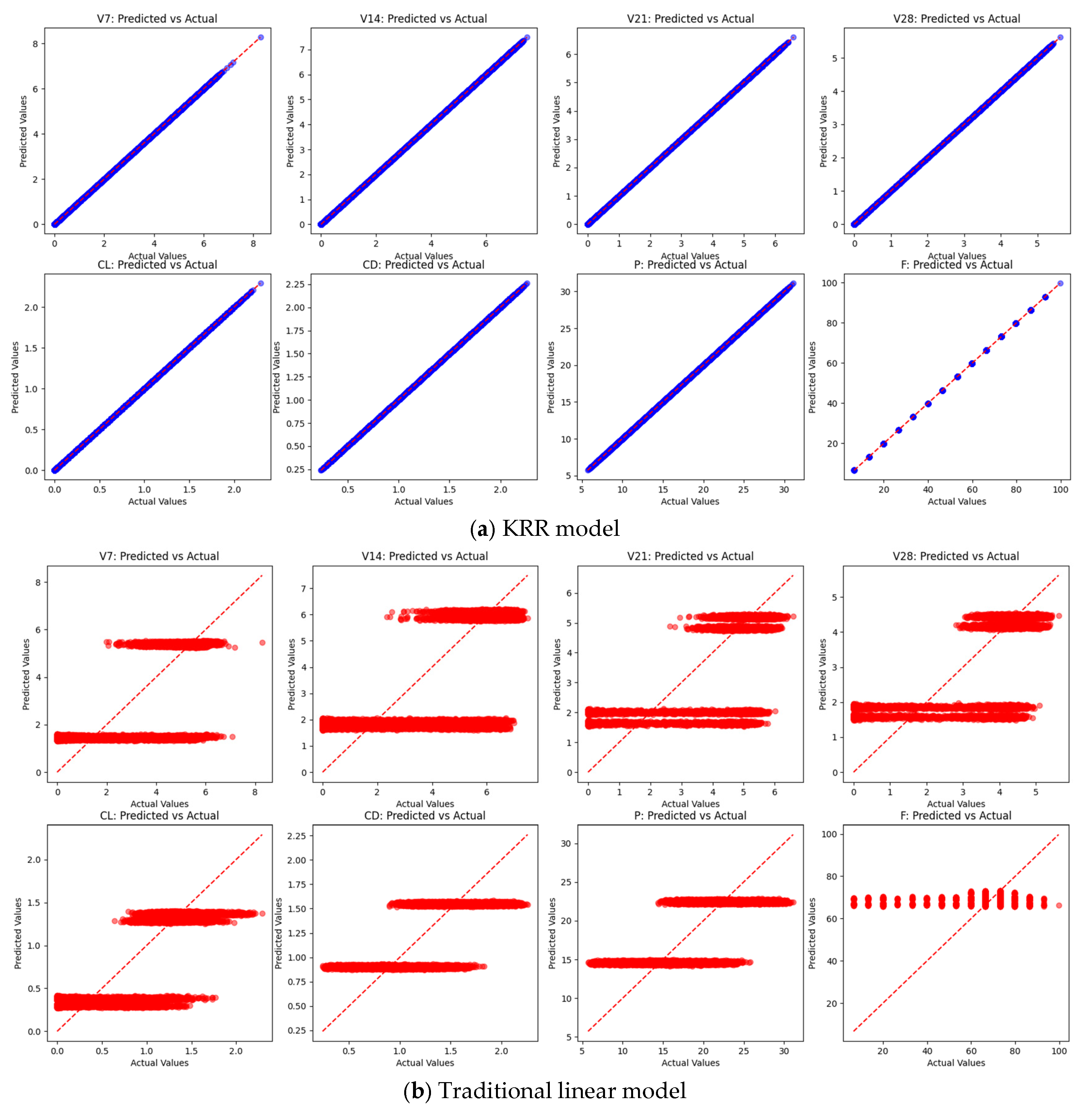
3.1. Fit Results and Comparison

In this field, due to the lack of prior research on modeling the relationship between input and output parameters, the traditional linear regression model was adopted as the benchmark method. The lines in Figure 15 are the ideal result, and each dot shows a group of data. As shown in the plot, linear regression cannot fit the complex relationships in the fluid well, while the improved machine learning method based on KRR can achieve a good fit. Moreover, the results of K-fold cross-validation indicate that there is no overfitting.

Table 5. Evaluation parameters of fitting results.

Parameter	MSE	RMSE	MAE	R2	CV_RMSE_Mean	CV_RMSE_Std
V7	1.99188 × 10−12	1.41134 × 10−6	1.08746 × 10−6	1	1.41115 × 10−6	2.33328 × 10−8
V14	2.79998 × 10−12	1.67331 × 10−6	1.27968 × 10−6	1	1.67308 × 10−6	2.79461 × 10−8
V21	2.27284 × 10−12	1.5076 × 10−6	1.16655 × 10−6	1	1.50745 × 10−6	2.06001 × 10−8
V28	1.7352 × 10−12	1.31727 × 10−6	1.04012 × 10−6	1	1.31719 × 10−6	1.47638 × 10−8
Cl	1.17433 × 10−13	3.42684 × 10−7	2.77535 × 10−7	1	3.42625 × 10−7	6.35703 × 10−9
Cd	8.95391 × 10−14	2.99231 × 10−7	2.48035 × 10−7	1	2.99194 × 10−7	4.69762 × 10−9
ΔP	1.40444 × 10−11	3.74759 × 10−6	3.09747 × 10−6	1	3.74706 × 10−6	6.26793 × 10−8
f	1.57333 × 10−10	1.25433 × 10−5	7.53052 × 10−6	1	1.25345 × 10−5	4.68339 × 10−7

shows the high effectiveness of the model. Not only does the result validate the effectiveness of the model, but it also indicates that the model can perfectly fit the complex characteristics of the bluff body of the vortex flowmeter. This model has high accuracy in predicting output parameters, providing a strong theoretical basis for subsequent optimization design and practical applications.

3.2. Correlation Analysis

3.2.1. GRA

The specific values of GRA’s r_i are shown in

Table 6. GRA table.

Parameters	V7	V14	V21	V28	ΔP	f	Cl	Cd
a	0.765	0.772	0.781	0.787	0.789	0.791	0.772	0.790
b	0.721	0.725	0.730	0.734	0.725	0.719	0.732	0.730
c	0.733	0.736	0.741	0.743	0.733	0.726	0.742	0.738
d	0.787	0.801	0.824	0.840	0.864	0.908	0.800	0.852
φ	0.766	0.772	0.781	0.788	0.792	0.791	0.773	0.793
θ	0.790	0.803	0.827	0.844	0.870	0.931	0.801	0.856
shape1	0.610	0.620	0.631	0.638	0.633	0.664	0.629	0.632
shape2	0.614	0.620	0.631	0.638	0.633	0.664	0.629	0.632

.

Through Grey Relational Analysis (GRA), we conducted a detailed evaluation of the correlation between input parameters and output parameters. The results indicate that size parameters have a more significant impact on output parameters than shape parameters. Specifically, the trailing edge angle (θ) and upstream width (d) exhibit an extremely strong correlation with frequency (r > 0.9), suggesting that these parameters play a key role in the formation and stability of vortex shedding. For instance, as θ and d increase, the frequency also increases, which is consistent with the theoretical principles of boundary layer separation and vortex shedding in fluid mechanics. For other input parameters, such as transition edge length (a) and downstream width (c), their impact on output parameters is relatively smaller but still notable. These results provide important references for subsequent parameter optimization.

3.2.2. Objective Function Analysis

As shown in Figure 11, the samples were grouped according to shape. And it also shows the relationship between the group number and the shape. Due to the limitation that all samples were taken from the simulation data of the flow rate of 5 m/s, the linearity of the vortex was not systematically analyzed in this study. Therefore, for the input parameters, only the objective function for flow monitoring point V₁₄ is established and divided into five intervals. The objective function has three output variables: the average data of each interval sampling point, the maximum value, and the variance. Meanwhile, draw a line graph of six structural parameters and three output variables of the objective function.

Figure 16 shows the relationship between a and V₁₄. The increase in parameter a will suppress the influence of the shape of the countercurrent surface (for example, the velocity of groups I, II, and IV reaches the maximum value when a = 1.5 mm), indicating that the guiding effect of a on the airflow dominates the output performance.

Figure 17 shows the relationship between b and V₁₄. On the contrary, parameter b showed similar monotonicity in groups II and III (the maximum velocity was reached at b = 17 mm), while groups I and IV reached an extreme value at b = 19 mm, which may be related to the pressure field distribution caused by the difference in the shape of the bluff body.

Figure 18 shows the relationship between c and V₁₄. When the countercurrent surface is concave, when the parameter c increases to 3.5 mm, the maximum value of V₁₄ in group III drops by 6.9%, while the mean and variance are almost unchanged, indicating that the turbulent separation characteristics change abruptly and the minimum value of V₁₄ drops sharply under this shape. With the increase in the arc of the countercurrent surface, the maximum value of V₁₄ will decrease sharply in a certain range. As the radius increases, the shape gradually deviates from the trapezoidal bluff body and becomes more similar to a semicircular bluff body.

Figure 19 shows the relationship between a and V₁₄. In the traditional trapezoidal bluff body, the velocity signal is the largest when d = 14 mm [8]. It can be seen that this conclusion is generally applicable when the onstream surface is perpendicular to the flow velocity direction, and it is not universally applicable. d should also be analyzed in detail when optimizing the structure of the curved bluff body. Groups I and III have the maximum velocity when d = 13.5, when the mean value reaches the maximum and the variance reaches the minimum, so it can be concluded that: when the oncoming surface is convex, the signal intensity is the strongest when d = 13.5.

Figure 20 shows the relationship between θ and V₁₄. With the increase in the radius of the oncoming surface, the maximum value of V₁₄ will first decrease and then rise in a certain range when the oncoming surface is concave. After that, the change is not obvious. As the radius increases, the shape gradually deviates from the trapezoidal bluff body.

Figure 21 shows the relationship between φ/φ₀ and V₁₄. When the countercurrent surface is convex, the maximum value of V₁₄ increases first and then decreases with the increase in the radius of the onstream surface.

3.2.3. CFD Analysis

Figure 22a–d illustrates the velocity contour maps of four specific shapes. Among them, the forward convex arc results in a smaller deceleration zone in front of the bluff body and lower maximum velocities on both sides of the bluff body while the width of the vortex street increases. It is speculated that the convex arc may have a better guiding effect on the flow, directing it toward the sides, thereby making the actual effective length greater than d. The convex arc on the counterflow surface leads to a smaller low-speed zone behind the bluff body and a larger vortex street length.

3.2.4. Correlation Discussion

The following are the conclusions of the correlation of input–output parameters:

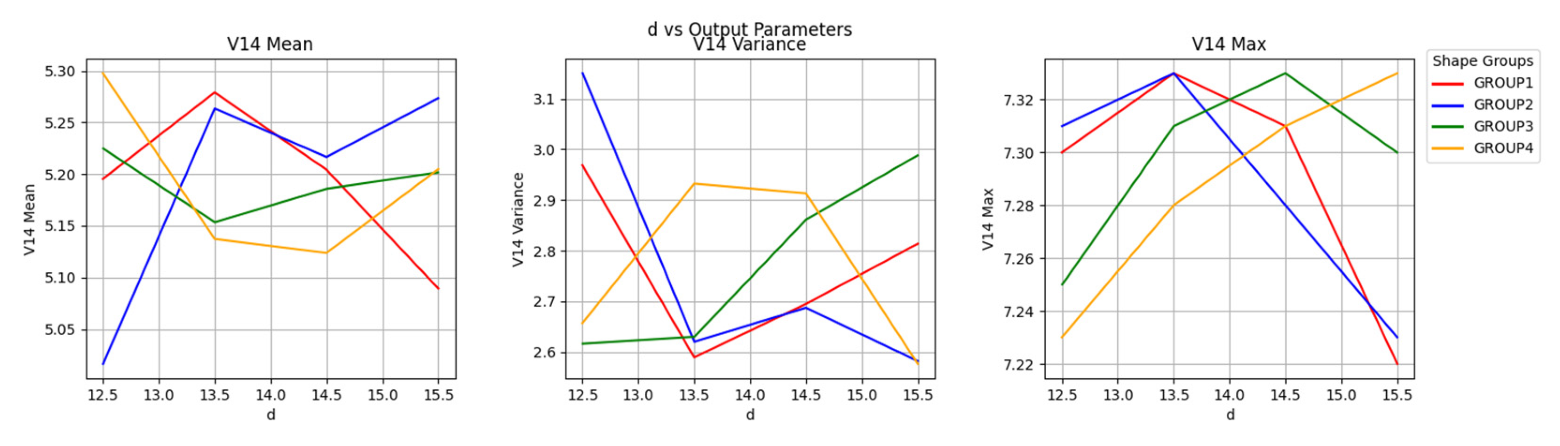
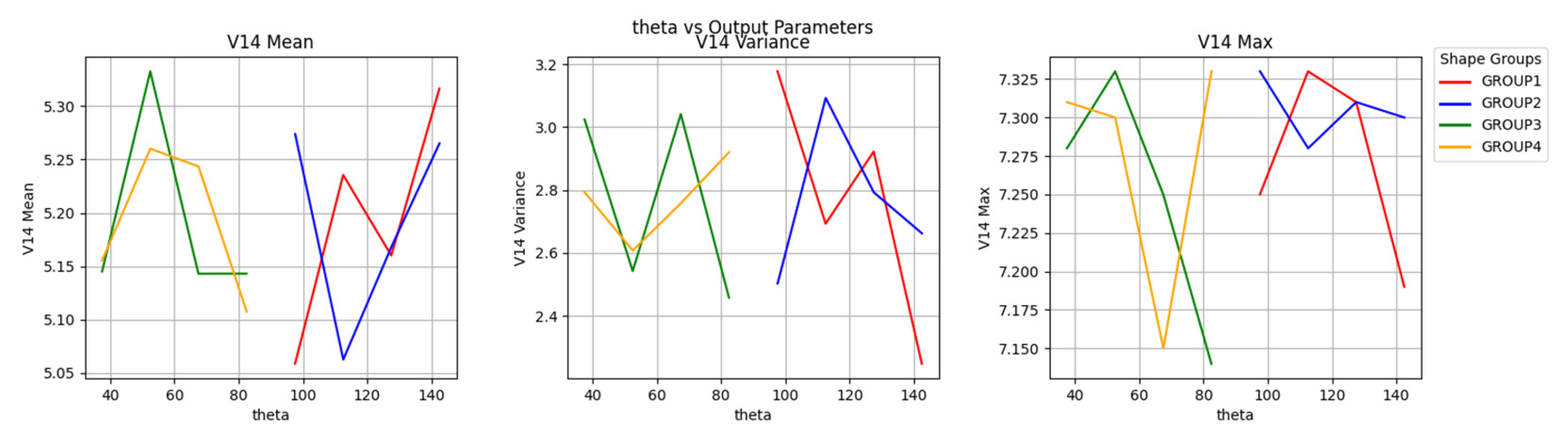
• The results of GRA indicate that the trailing edge angle (θ) and upstream width (d) have the strongest correlation with frequency (r > 0.9). This strong correlation suggests that these parameters play a significant role in determining the vortex shedding frequency, which is a key performance indicator for vortex flowmeters. Specifically, an increase in θ and d leads to an increase in frequency. This finding aligns with the theoretical principles of boundary layer separation and vortex shedding, where the geometry of the bluff body directly influences the formation and stability of vortices.
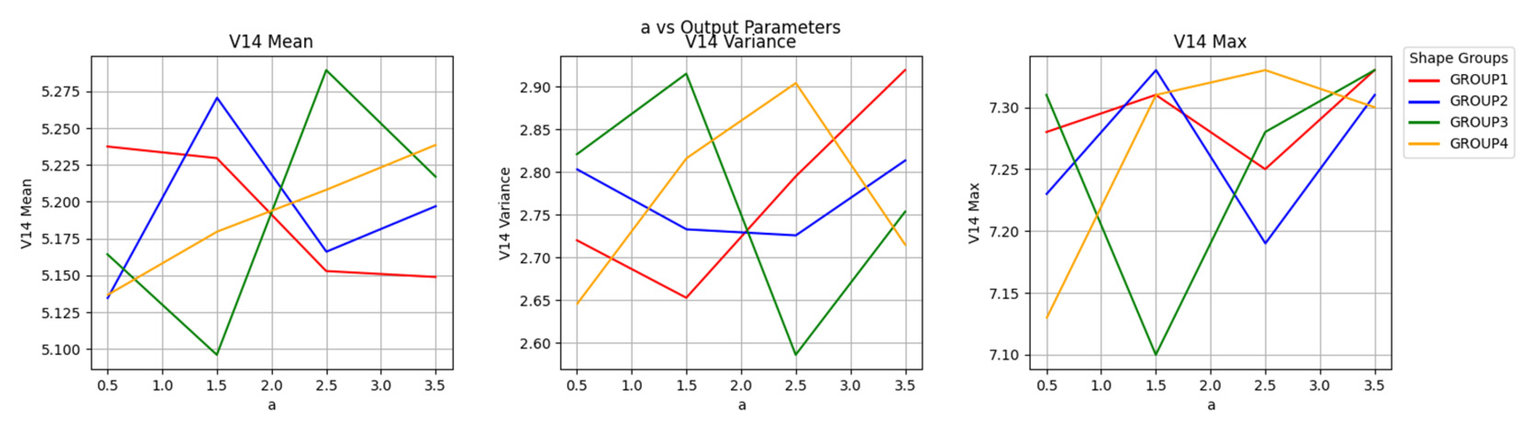
• The transition edge length (a) significantly affects the velocity distribution around the bluff body. The results indicate that increasing a suppresses the influence of the shape of the countercurrent surface, suggesting that the guiding effect of a on the airflow dominates the output performance. This highlights the crucial role of a in directing the flow around the bluff body, thereby influencing overall performance.
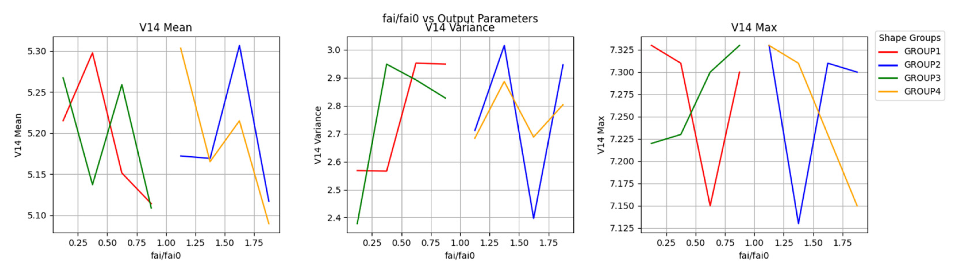
• The bluff body length (b) also significantly affects the velocity distribution and vortex street characteristics. For instance, in some cases, an increase in b to 17 mm results in the maximum value of V14, while in other scenarios, an increase to 19 mm leads to an extreme value of V14. This suggests that the pressure field distribution, influenced by the shape of the bluff body, plays a role in these observations. Therefore, careful consideration of the value of b is necessary to optimize the performance of vortex flowmeters.
• The downstream width (c) also impacts the velocity distribution, especially when the countercurrent surface is concave. The results show that increasing c to 3.5 mm leads to a significant drop in the maximum value of V₁₄, while the mean and variance remain almost unchanged. This suggests that the turbulent separation characteristics change abruptly under this condition, resulting in a sharp drop in the minimum value of V₁₄. This finding underscores the importance of carefully selecting the downstream width to optimize the performance of vortex flowmeters.
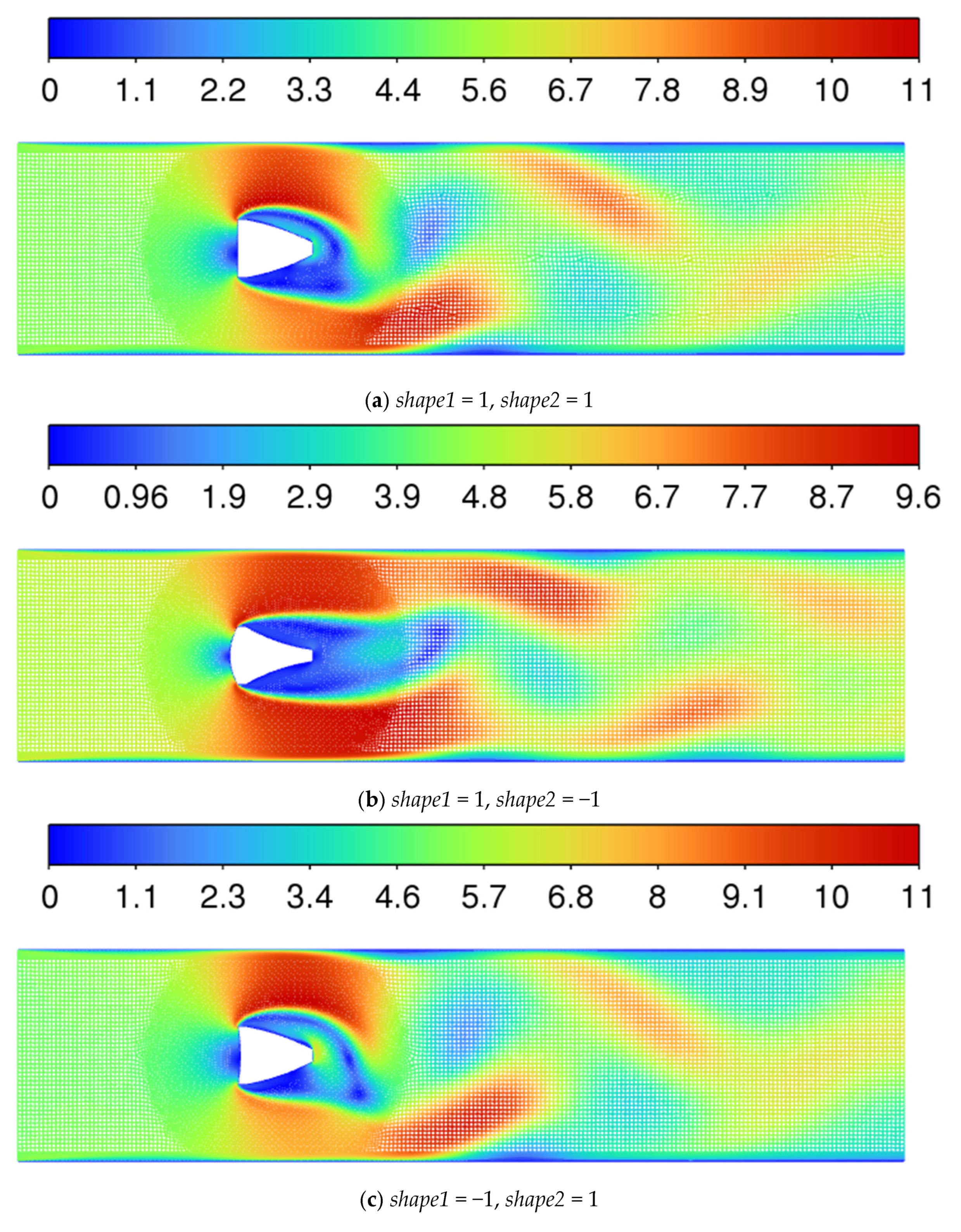
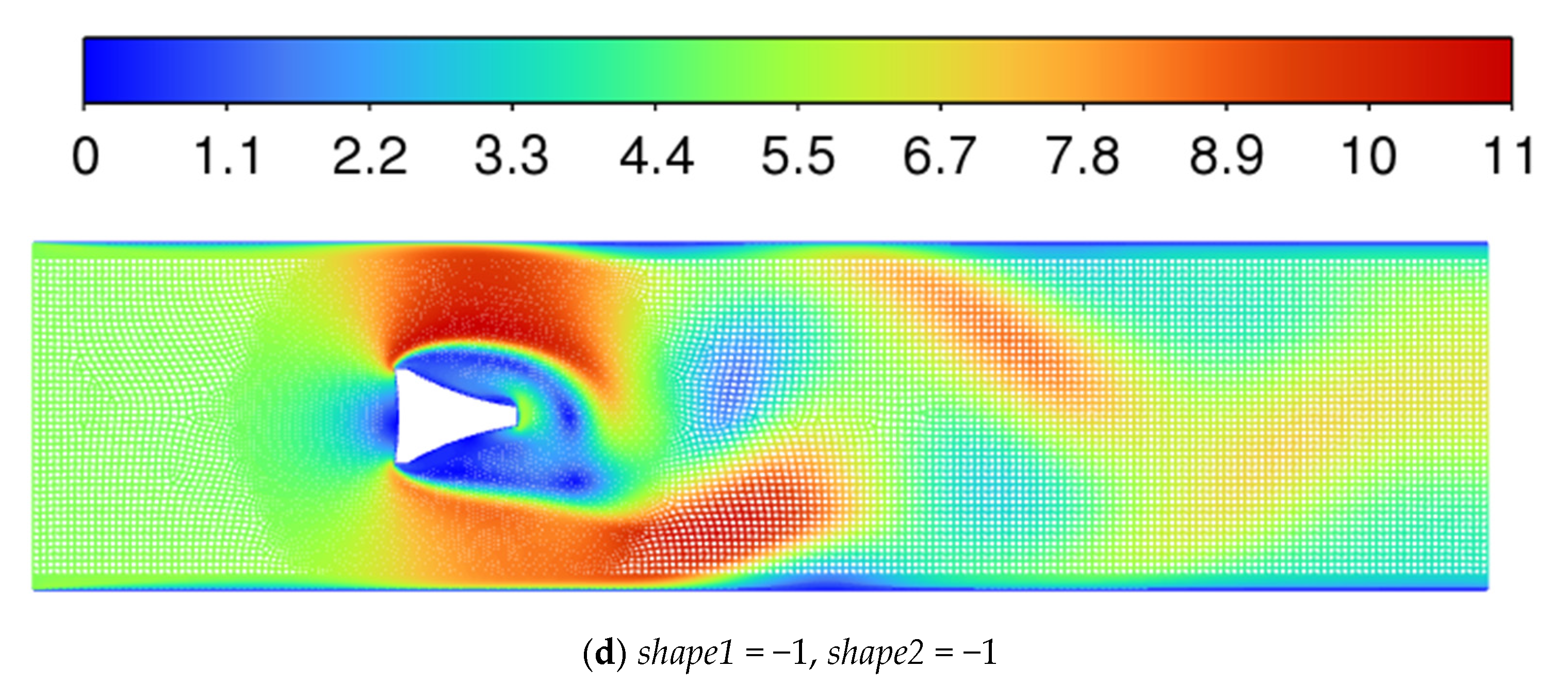
• The shape parameters (shape1 and shape2) define the curvature of the forward and backward arcs of the bluff body, respectively. These parameters influence the flow characteristics around the bluff body, thereby affecting vortex formation and stability. The results show that the shape parameters have a moderate correlation with the performance indicators, indicating that the curvature of the arcs plays a role in determining flow dynamics. For example, a convex forward arc (shape1 = 1) results in a smaller deceleration zone in front of the bluff body and lower maximum velocities on both sides while increasing the width of the vortex street. This suggests that the convex arc may have a better guiding effect on the flow, directing it toward the sides and thereby increasing the actual effective length of the bluff body.
• Similarly, a convex backward arc (shape2 = 1) leads to a smaller low-speed zone behind the bluff body and a larger vortex street length. This indicates that the curvature of the backward arc influences flow separation and reattachment, thereby affecting the overall performance of the vortex flowmeter.

The findings from the correlation analysis provide a solid theoretical foundation for the design and optimization of vortex flowmeters. By understanding the relationships between geometric parameters and performance indicators, engineers can make informed decisions to optimize the design of bluff bodies for specific applications. For example, adjusting the trailing edge angle (θ), upstream width (d), and bluff body length (b) can significantly enhance vortex shedding frequency, thereby improving the accuracy and reliability of the flowmeter.

4. Conclusions

In this paper, the method of batch serial simulation effectively improves the simulation speed, which is beneficial for accelerating the construction of machine learning databases. In this study, by improving machine learning and incorporating iterative methods, a fitting method was successfully found that can accurately fit the relationship between the eight output parameters and eight input parameters of the vortex street. In addition, the influence of different input parameters on the output parameters was analyzed. These findings provide an important theoretical basis for the design and optimization of vortex flowmeter bluff bodies, which can help improve their measurement accuracy and reliability. However, this fitting method may overfit other shapes of bluff bodies. In the future, convolutional neural networks can be used to better fit other shapes of bluff bodies. Meanwhile, this paper only analyzes the relationship and trends between input and output parameters and does not propose a detailed and rigorous mechanism to explain them. In the future, combined with further simulations, a detailed mechanism can be proposed to explain the relationship between shape, structural parameters, and output parameters from the perspective of fluid mechanics.

References

1. Kármán, T.V. Über den Mechanismus des Wiederstandes, den ein bewegter Körper in einer Flüssigkeit erfahrt. Nachrichten Ges. Wiss. Göttingen Math. Phys. Kl. 1912, 1912, 547–556. [Google Scholar]
2. Miau, J.J.; Yang, C.C.; Chou, J.H.; Lee, K.R. A T-shaped vortex shedder for a vortex flow-meter. Flow Meas. Instrum. 1993, 4, 259–267. [Google Scholar] [CrossRef]
3. Coulthard, J.; Yan, Y. Comparisons of Different Bluff Bodies in Vortex Wake Transit Time Measurements. Flow Meas. Instrum. 1993, 4, 273–275. [Google Scholar] [CrossRef]
4. Baker, R.C. Flow Measurement Handbook; Cambridge University Press: New York, NY, USA, 2000. [Google Scholar]
5. Miller, R.W.; De Carlo, J.P.; Gullen, J.T. A vortex flowmeter—Calibration results and application experience. Proc. Flow-Con. 1977, 2, 341–371. [Google Scholar]
6. Kremlevskiy, P.P. Flowmeters and Counters; Mashinostroenie: Leningrad, Russia, 1989. [Google Scholar]
7. Sun, Z. Numerical Simulation and Experimental Study of Vortex Frequency Detection Method for Vortex Flowmeter Based on Differential Pressure Principle. Master’s Thesis, Central South University, Changsha, China, 2004. [Google Scholar]
8. Venugopal, A.; Agrawal, A.; Prabhu, S.V. Influence of blockage and shape of a bluff body on the performance of vortex flowmeter with wall pressure measurement. Measurement 2011, 44, 954–964. [Google Scholar] [CrossRef]
9. Du, P. Numerical Simulation of Vortex Shedding Frequency in Vortex Flowmeter. Master’s Thesis, Northeast Petroleum University, Daqing, China, 2015. [Google Scholar]
10. Venugopal, A.; Agrawal, A.; Prabhu, S.V. On the linearity, turndown ratio, and shape of the bluff body for vortex flowmeter. Measurement 2019, 137, 477–483. [Google Scholar] [CrossRef]
11. Krivonogov, A.; Kartashev, A.; Kartasheva, M. System for Computer Simulation and Optimization of Vortex Flows. In Proceedings of the 2020 International Conference on Industrial Engineering, Applications and Manufacturing (ICIEAM), Sochi, Russia, 15–17 July 2020; pp. 1–6. [Google Scholar]
12. Rzasa, M.R.; Czapla-Nielacna, B. Analysis of the influence of the vortex shedder shape on the metrological properties of the vortex flow meter. Sensors 2021, 21, 4697. [Google Scholar] [CrossRef]
13. Končar, B.; Sotošek, J.; Bajsić, I. Experimental verification and numerical simulation of a vortex flowmeter at low Reynolds numbers. Flow Meas. Instrum. 2022, 88, 102278. [Google Scholar] [CrossRef]
14. Shen, C.; Feng, S.; Zhu, Y.; Jin, K. Numerical simulation of pressure tapping location of precession vortex flowmeter based on CFX. J. Drain. Irrig. Mach. Eng. 2023, 41, 487–492. [Google Scholar]
15. Lur’e, M.S.; Lur’e, O.M.; Slashchinin, D.G.; Frolov, A.S.; Chernov, V.A. Modernization of the Vortex Flowmeter with a Trapezoidal Bluff Body and a Feedback Channel. Steel Transl. 2024, 54, 288–292. [Google Scholar] [CrossRef]
16. Farsad, S.; Parpanchi, S.M.; Rezaei, M. Experimental study of vortex shedding phenomenon induced by various bluff body geometries for use in vortex flowmeters. Eur. J. Mech.—B/Fluids 2025, 111, 188–200. [Google Scholar] [CrossRef]
17. Zhang, W.; Kong, M.; Zhang, Y.; Fathollahi-Fard, A.M.; Tian, G. A revised deep reinforcement learning algorithm for parallel machine scheduling problem under multi-scenario due date constraints. Swarm Evol. Comput. 2025, 92, 101808. [Google Scholar]
18. Ren, Y.; Meng, L.; Tian, G.; Li, Z.; Li, Y. An efficient m-step lookahead rollout algorithm for profit-oriented selective disassembly sequence planning with operation stochastic failure. Eng. Appl. Artif. Intell. 2025, 145, 110173. [Google Scholar] [CrossRef]
19. Ling, J.; Templeton, J. Evaluation of machine learning algorithms for prediction of regions of high Reynolds averaged Navier Stokes uncertainty. Phys. Fluids 2015, 27, 085103. [Google Scholar]
20. Duraisamy, K.; Iaccarino, G.; Xiao, H. Turbulence modeling in the age of data. Annu. Rev. Fluid Mech. 2019, 51, 357–377. [Google Scholar] [CrossRef]
21. Zhu, L.; Zhang, W.; Kou, J.; Liu, Y. Machine learning methods for turbulence modeling in subsonic flows around airfoils. Phys. Fluids 2019, 31, 015105. [Google Scholar] [CrossRef]
22. Hadi, A.A.; Ahmed, S.R.; Abbas, S.K.; Al-Sharify, Z.T.; Fuqdan, A.I.; Ahmad, B.A.; Khider, A.I.; Algburi, S.; Shin, J. Machine Learning Techniques for Turbulence Analysis and Simulation. In Proceedings of the 2024 8th International Symposium on Innovative Approaches in Smart Technologies (ISAS), İstanbul, Türkiye, 12–14 September 2024; pp. 1–7. [Google Scholar]
23. Raibaudo, C.; Zhong, P.; Noack, B.R.; Martinuzzi, R.J. Machine learning strategies applied to the control of a fluidic pinball. Phys. Fluids 2020, 32, 015108. [Google Scholar]
24. Jin, X.; Cheng, P.; Chen, W.-L.; Li, H. Prediction model of velocity field around circular cylinder over various Reynolds numbers by fusion convolutional neural networks based on pressure on the cylinder. Phys. Fluids 2018, 30, 047105. [Google Scholar] [CrossRef]
25. Tang, H.; Rabault, J.; Kuhnle, A.; Wang, Y.; Wang, T. Robust active flow control over a range of Reynolds numbers using an artificial neural network trained through deep reinforcement learning. Phys. Fluids 2020, 32, 053605. [Google Scholar]
26. Li, H.; Tan, J.; Gao, Z.; Noack, B.R. Machine learning open-loop control of a mixing layer. Phys. Fluids 2020, 32, 111701. [Google Scholar]
27. Wu, Z.; Fan, D.; Zhou, Y.; Li, R.; Noack, B.R. Jet mixing optimization using machine learning control. Exp. Fluids 2018, 59, 131. [Google Scholar]
28. Guo, X.; Li, W.; Iorio, F. Convolutional neural networks for steady flow approximation. In Proceedings of the 22nd ACM SIGKDD International Conference on Knowledge Discovery & Data Mining, San Francisco, CA, USA, 13–17 August 2016; pp. 481–490. [Google Scholar]
29. Sekar, V.; Khoo, B.C. Fast flow field prediction over airfoils using deep learning approach. Phys. Fluids 2019, 31, 057103. [Google Scholar]
30. Jiang, C.; Yang, R.; Xu, Q.; Yao, H.; Ho, T.-Y.; Yuan, B. A Cooperative Multiagent Reinforcement Learning Framework for Droplet Routing in Digital Microfluidic Biochips. IEEE Trans. Comput. Aided Des. Integr. Circuits Syst. 2023, 42, 3007–3020. [Google Scholar]
31. Zhang, Y.; Sung, W.-J.; Mavris, D. Application of Convolutional Neural Network to Predict Airfoil Lift Coefficient. J. Aircraft 2018, 55, 1023–1034. [Google Scholar]
32. Thummar, D.; Reddy, Y.J.; Venugopal, A. Machine learning for vortex flowmeter design. IEEE Trans. Instrum. Meas. 2021, 71, 1–8. [Google Scholar]
33. Sudharsan, B.; Peeples, M.; Shomali, M. Hypoglycemia prediction using machine learning models for patients with type 2 diabetes. J. Diabetes Sci. Technol. 2015, 9, 86–90. [Google Scholar]
34. Georga, E.I.; Protopappas, V.C.; Ardigò, D.; Polyzos, D.; Fotiadis, D.I. A glucose model based on support vector regression for the prediction of hypoglycemic events under free-living conditions. Diabetes Technol. Ther. 2013, 15, 634–643. [Google Scholar]
35. Si, X.; Shen, Y.; Bao, J. Simulation study of triangular vortex generator in vortex flowmeter based on CFD. Electron. Meas. Technol. 2020, 43, 6–9. [Google Scholar]
36. Mckay, M.D.; Beckman, R.J.; Conover, W.J. A comparison of three methods for selecting values of input variables in the analysis of output from a computer code. Technometrics 1979, 21, 239–245. [Google Scholar]
37. Venugopal, A.; Agrawal, A.; Prabhu, S.V. Vortex dynamics of a trapezoidal bluff body placed inside a circular pipe. J. Turbul. 2018, 19, 1–24. [Google Scholar]
38. Yang, L.J.; Zhang, B.H.; Ye, X.Z. Fast Fourier Transform (FFT) and its applications. Opto-Electron. Eng. 2004, 2004, 1–3+7. [Google Scholar]
39. Cawley, G.C.; Talbot, N.L.C. Optimizing sparse kernel ridge regression hyperparameters based on leave-one-out cross-validation. In Proceedings of the 2008 IEEE International Joint Conference on Neural Networks, Hong Kong, China, 1–8 June 2008; IEEE: Piscataway, NJ, USA, 2008; pp. 2981–2987. [Google Scholar]
40. Caponnetto, A.; De Vito, E. Optimal rates for the regularized least-squares algorithm. Found. Comput. Math. 2007, 7, 331–368. [Google Scholar] [CrossRef]
41. Vapnik, V.N. The Nature of Statistical Learning Theory; Springer: New York, NY, USA, 1995. [Google Scholar]
42. Orsenigo, C.; Vercellis, C. Kernel ridge regression for out-of-sample mapping in supervised manifold learning. Expert Syst. Appl. 2012, 39, 7757–7762. [Google Scholar] [CrossRef]
43. Cawley, G.C.; Talbot, N.L.C. On over-fitting in model selection and subsequent selection bias in performance evaluation. J. Mach. Learn. Res. 2010, 11, 2079–2107. [Google Scholar]
Figure 1. Schematic diagram of Karman vortex.
Symmetry 17 00510 g001
Figure 2. Boundary layer separation phenomenon in bluff bodies.
Symmetry 17 00510 g002
Figure 3. Size and shape parameters of bluff bodies.
Symmetry 17 00510 g003
Figure 4. Sampling interval.
Symmetry 17 00510 g004
Figure 5. Schematic diagram of flow channel size and coordinate system.
Symmetry 17 00510 g005
Figure 6. Schematic diagram of naming selection.
Symmetry 17 00510 g006
Figure 7. Mesh grid of two-dimensional flow field modeling.
Symmetry 17 00510 g007
Figure 8. Serial simulation verification.
Symmetry 17 00510 g008
Figure 9. Residuals of CFD.
Symmetry 17 00510 g009
Figure 10. Schematic diagram of speed detection point.
Symmetry 17 00510 g010
Figure 11. Process of K-fold cross-validation.
Symmetry 17 00510 g011
Figure 12. Whole researching process flowchart.
Symmetry 17 00510 g012
Figure 13. Data processing flowchart.
Symmetry 17 00510 g013
Figure 14. Model building process.
Symmetry 17 00510 g014
Figure 15. Chart of predicted values and actual values.
Symmetry 17 00510 g015
Figure 16. a-V14 correlation line chart.
Symmetry 17 00510 g016
Figure 17. b-V14 correlation line chart.
Symmetry 17 00510 g017
Figure 18. c-V14 correlation line chart.
Symmetry 17 00510 g018
Figure 19. d-V14 correlation line chart.
Symmetry 17 00510 g019
Figure 20. θ-V14 correlation line chart.
Symmetry 17 00510 g020
Figure 21. φ/φ0-V14 correlation line chart.
Symmetry 17 00510 g021
Figure 22. Velocity contour maps of four shapes.
Symmetry 17 00510 g022aSymmetry 17 00510 g022b