Optimal Control of Stochastic Dynamic Systems with Semi-Markov Parameters

Abstract

This paper extends classical Markov switching models. We introduce a generalized semi-Markov switching framework in which the system dynamics are governed by an Itô stochastic differential equation. Of note, the optimal control synthesis problem is formulated for stochastic dynamic systems with semi-Markov parameters. Further, a system of ordinary differential equations is derived to characterize the Bellman functional and the corresponding optimal control. We investigate the case of linear dynamics in detail, and propose a closed-form solution for the optimal control law. A numerical example is presented to illustrate the theoretical results.

1. Introduction

Optimal control synthesis plays a critical role in managing the dynamics of controlled objects or processes. This is particularly relevant when the dynamic behavior is described by Ito stochastic differential equations (SDEs). The choice of Ito SDE is due to their prevalence as applied models and their widespread use in biology, chemistry, telecommunications, etc. The main type of random perturbations in stochastic differential equations is the symmetric Wiener process, the trajectories of which have the reflection property, which very well characterizes the symmetry of this process. The symmetry of the solution of the stochastic differential equation is also well reflected in the example of this work, where the symmetry of the solution trajectories is traced relative to the so-called averaged trajectory, and optimal control does not violate this property. The paper [1] considers the optimal control of a linear SDE of general type perturbed by a random process with independent increments and a quadratic quality functional. It is shown that under certain conditions the optimal control is linear and can be determined by solving an additional vector quadratic problem. The optimal solution of the deterministic problem with feedback is obtained. In paper [2], the theory of optimal control for stochastic systems whose performance is measured by the exponent of an integral form is developed. In paper [3], the problem of the existence of optimal control for stochastic systems with a nonlinear quality functional is solved. The main model in the work [4] is the linear autonomous SDE in the form

$$g(x,u)=A_{0}x+B_{0}u+w_k(A_{1}x+B_{1}u),$$

(1)

where $w_k\sim i.i.d$ with $E{w}_k=0,Var\left(w_k\right)=1$. Notably, the results of the paper are devoted to the quadratic quality functional and necessary and sufficient conditions for the stability of the systems (1), and the stability conditions are formulated in terms of Riccati-type jumping operator properties. Note that the linear case (1) is most often considered as a first approximation of the dynamics of a real phenomenon, since the optimal control in this case can be found in closed form and the approximations of the optimal control can be compared with the exact values.

In article [5], the main attention is focused on SDE with external switches. In this paper, a number of important remarks are made on the calculation of the product (infinitesimal) operator of a random process given by a SDE with Markov switches.

In article [6], SDE with external switches and Poisson perturbations are discussed. Using the Belman equation, sufficient conditions for the existence of optimal control for a general quality function are found, and a closed form of optimal control is found for the linear case with a quadratic quality function.

The transition from difference equations to differential equations gives rise to a number of complications in the synthesis of optimal control, since it leads to a transition from solving more complex dynamical systems such as the analog of the Lyapunov equation for nonautonomous systems. Further, the presence of random variables of different structures leads to the use of the infinitesimal operator [7,8], the calculation of which depends on the nature of the random variables that affect the calculation of the infinitesimal operator.

In this paper, we will focus on the use of semi-Markov processes [8] as the main source of external random disturbances. Noteworthy, the use of semi-Markov processes significantly extends the range of application of theoretical results for many applied problems, since the condition of exponential distribution of the time spent in the state ${\theta }_n$ for continuous Markov processes $\xi \left(t\right), t\ge 0,$ is very strict for many applied problems. A description based on a Markov process will be incorrect if, for example, an assumption is made about the minimum time spent in a particular state $P({\theta }_n>t_{min})=1$, where $t_{min}$ is the minimum time spent in the state. In this case, the use of semi-Markov processes is more efficient, since it allows us to control the properties of the residence time, the size of the jump ${\widehat{\xi }}_n$ and the interdependence between them based on the semi-Markov kernel $Q(y,B,t)$ [8]. The use of Markov processes greatly simplifies the study of the system, since it requires estimation only on the basis of the intensities of the Markov process $\lambda \left(y\right)$, and usually when studying systems with external Markov disturbances it is assumed that

$$0<{\lambda }_{min}\le \lambda \left(y\right)\le {\lambda }_{max}<\infty ,\forall y\in \mathbf{Y}.$$

In this study, we will not focus on the asymptotic properties of the random process $x\left(t\right)$, $t\ge 0$, but will consider the problem of synthesizing optimal control on a finite interval $[0,T]$, so the article will not consider additional conditions on the semi-Markov process that ensure its ergodicity [7,9,10].

Note that the study of optimal control with semi-Markovian processes has been receiving attention since the last quarter of the 20th century, when it became clear that the exponential distribution cannot be considered as the basic distribution for the transition time in many cases. For example, in the work [11], the optimization of the system in the presence of random shocks, which in turn are described by semi-Markov processes, is considered. The work gives an example of optimal replacement of the levels of the system and constructs a replacement algorithm for a countable set of states of the semi-Markov process. Models for finding the optimal general repair policy are considered in [12], and the semi-Markov process in this case describes construction errors, and the policy change is based on minimizing the budget on the one hand and fulfilling all construction requirements on the other. In [13], the authors considered the possibility of using semi-Markov models to solve the output-feedback control problem for general semi-Markov jump systems with a memory-dynamic event-triggered protocol. The authors of this article proposed a description of the system using a differential equation with a semi-Markovian component for the derivative of the process, i.e., the dynamics of the process will depend integrally on the dynamics of the semi-Markovian process. The main statements of this work provide sufficient conditions for the existence of optimal control for systems with semi-Markov parameters and an example of finding optimal control is given. A somewhat similar result for the case of asynchronous control was investigated in work [14]. The paper also provides several sufficient conditions for stochastic controllability of the system and considers a number of model examples with implementations of the semi-Markov process.

As noted in many works, the use of semi-Markov processes is of great practical importance, since the use of these models allows for a more accurate description of real processes. For example, in work [12] the authors used a semi-Markov process to find the optimal policy in construction, in work [15] the authors used semi-Markov processes with the corresponding problem of optimizing a portfolio of securities. Practically, this explains the use of Markov models with exponential time of stay in states is a good theoretical model, but for practical reasons it has a number of limitations associated with the moments of switching. As noted in paper [12], the policy change occurs at discrete moments of time and has a uniform distribution over a finite horizon, so the use of the Markov model in this case is inappropriate.

Instead, the main attention will be paid to the elementary study of the dynamics of the main process $x\left(t\right),t\in [0,T],$ at a fixed value of the external perturbation $\xi \left(t\right)=y,y\in \mathbf{Y}$, which allows us to more effectively study the optimal control based on the methods proposed for Markov processes. Section 2 of the article describes the problem statement and justifies the existence of a solution that is unique up to stochastic equivalence. In Section 3, sufficient conditions for the existence of a solution to the optimal control problem are established, and in Section 4, a method for finding it in the general case is described. Section 5 is devoted to the synthesis of optimal control for a linear system with a quadratic performance index, and in Section 6, a system of Riccati differential equations is presented for finding the matrix functions that form optimal control. The last section, Section 7, contains a model example that illustrates the stages of optimal control synthesis under the condition that the time spent in a state is determined by ${\theta }_n=t_{min}+Poiss\left(\lambda \left(y\right)\right)$, i.e., the time spent in a state is discrete and with probability 1 greater than $t_{min}$.

2. Problem Statement

Consider a stochastic dynamical system defined on a probabilistic basis $(\Omega ,\mathfrak{F},F,\mathbf{P})$ [7,16]. The system is governed by the stochastic differential equation (SDE):

$$dx\left(t\right)=a(t,\xi \left(t\right),x\left(t\right),u\left(t\right))dt+b(t,\xi \left(t\right),x\left(t\right),u\left(t\right))dw\left(t\right),t\in {\mathbb{R}}_{+},$$

(2)

with initial conditions

$$x\left(0\right)=x_0\in {\mathbb{R}}^m,\xi \left(0\right)=y\in \mathbf{Y}.$$

(3)

Here, $\xi \left(t\right),t\ge 0,$ is a semi-Markov process with values in $\mathbf{Y}$, which is characterised by generator [9]

$$Q(y,B,t)=P(y,B)F_y\left(t\right),y\in \mathbf{Y},B\in {\beta }_{\mathbf{Y}},t\ge 0,$$

(4)

where $P(y,B)$ specifies the distribution of jumps of the nested Markov chain ${\widehat{\xi }}_n,n\ge 0$ [8], $F_y\left(t\right)$ is the conditional distribution of time spent in the state y. The representation of the generator based on the splitting (4) greatly simplifies the main calculations in proving the main theoretical results of this paper, but allows for generalization to the general case of a semi-Markov kernel $Q(y,B,t)$; $x:\left[0,+\infty \right)\times \Omega \to {\mathbb{R}}^m$; $w\left(t\right)$, $t\ge 0,$ is a standard Wiener process; a control $u\left(t\right):=u(t,x\left(t\right)):[0,T]\times {\mathbb{R}}^m\to {\mathbb{R}}^m$ is m-measured function from the set of admissible controls U [17]; and the processes w and $\xi$ are independent [7,16].

As in works [16,18], we assume that the measured by the set of variables functions $a:{\mathbb{R}}_{+}\times \mathbf{Y}\times {\mathbb{R}}^m\times U\to {\mathbb{R}}^m$ and $b:{\mathbb{R}}_{+}\times \mathbf{Y}\times {\mathbb{R}}^m\times U\to {\mathbb{R}}^m$ satisfy the boundedness condition and the Lipschitz condition

$${\left|a(t,y,x,u)\right|}^2+{\left|b(t,y,x,u)\right|}^2\le {C(1+|x|}^2),$$

(5)

$$|a(t,y,x_1,u)-a(t,y,x_2,u){|}^2+|b(t,y,x_1,u)-b(t,y,x_2,u){|}^2\le L{|x_1-x_2|}^2,x_1,x_2\in {\mathbb{R}}^m.$$

(6)

The semi-Markov process $\xi$ has the following effect on the trajectories of the process x. Suppose that on the interval $[t_0=0,t_1)$, the process $\xi$ takes the value $y_1$. Then, the movement will occur due to the system

$$dx\left(t\right)=a(t,y_1,x\left(t\right),u\left(t\right))dt+b(t,y_1,x\left(t\right),u\left(t\right))dw\left(t\right),t\in {\mathbb{R}}_{+},x\left(0\right)=x_0\in {\mathbb{R}}^m.$$

(7)

According to [10,16], if the conditions (5) and (6) are met, the system (7) has on the interval $[0,t_1)$ a unique solution with a finite second moment up to stochastic equivalence.

Then, at time $t_1$, the value of the process $\xi$ changes: $y_1\to y_2$. Then, on the interval $[t_1,t_2)$, the motion will occur due to the system

$$dx\left(t\right)=a(t,y_2,x\left(t\right),u\left(t\right))dt+b(t,y_2,x\left(t\right),u\left(t\right))dw\left(t\right),t\in {\mathbb{R}}_{+},x\left(t_1\right)=x(t_1-)\in {\mathbb{R}}^m.$$

(8)

According to [10,16], if conditions (5) and (6) are met, system (8) has a unique solution with a finite second moment on the interval $[t_1,t_2)$.

Thus, conditions (5) and (6) guarantee the existence of a unique solution to the Cauchy problem, (2), and (3) on the interval $[0,+\infty )={\displaystyle \bigcup _{k=0}^{\infty }}[t_k,t_{k+1}),0=t_0,t_1,\dots ,t_k,\dots$, the second moment for which is finite. Thus, for the existence of a solution on $[0,\infty )$, we will assume that the semi-Markov process is defined on $[0,\infty )$, i.e., $\forall T>0:P\left(\xi \right(T\left)\mathrm{exist}\right)=1$.

3. Sufficient Conditions for Optimality

We introduce a sequence of functions $v_k(t,x):[t_k,T]\times {\mathbb{R}}^m\to {\mathbb{R}}^1,k\ge 0,$ and class $V:=\{v_k(t,x)\in C^{1,2}({\mathbb{R}}_{+}\times {\mathbb{R}}^m)\}$.

On the functions $v_k(t,x)\in V$, we define the weak infinitesimal operator (WIO)

$$\mathcal{L}{v}_k(t,x)=\underset{\Delta \to 0+}{lim}{\displaystyle \frac{1}{\Delta }}\{\mathbf{E}{v}_k(t+\Delta ,x(t+\Delta ,t_k,y,u))-v_k(t,x)\},$$

(9)

where $x\left(t\right)=x(t,t_k,y,u)$ is the strong solution (2) on the interval $t\in [t_k,t_{k+1})$ with control $u=u_k\in U$. Notice that WIO is natural extension of the right-hand side of the ordinary differential equation

$${\displaystyle \frac{dx}{dt}}=f(t,x)$$

in the case of stochastic systems.

The problem of optimal control is to find a control $u_k^0,k\ge 0,$ from the set U that minimizes the scalar quality functional [17]

$$I\left(u_k^0\right)=I^{u_k^0}(t,x)=\underset{u\in U}{inf}\left(\sum _{k=0}^N{\mathbf{E}}_{t_k,x_k}\left\{F\left(x\left(T\right)\right)+\underset{t}{\overset{T}{\int }}G(s,x\left(s\right),u\left(s\right))ds\right\}\right),$$

(10)

for some fixed $T>0$, $F\left(x\right)\ge 0, G(t,x,u)\ge 0$, ${\mathbf{E}}_{t,x}\left\{f\right\}=\mathbf{E}\{f/x\left(t\right)=x\}$, and $N=max\{k:t_k<T\}$.

To obtain sufficient conditions for optimality, we need to prove several auxiliary statements.

Lemma 1.

Let:

(1) 

There exists a unique solution to the Cauchy problem (2), and (3), whose second moment is finite for each t;

(2) 

A sequence of functions $v_k:[0,T]\times {\mathbb{R}}^m\to {\mathbb{R}}^1,k\ge 0,$ from class V exists;

(3) 

For $s\in [t_k,T)$, the WIO $\mathcal{L}{v}_k(s,x)$ is defined on the solutions of (2) and (3).

Then, for $\forall {\tilde{t}}_1,{\tilde{t}}_2\in [t_0,T]$ the following equality holds

$${\mathbf{E}}_{t_k,x_k}{v}_k({\tilde{t}}_2,x\left({\tilde{t}}_2\right))-{\mathbf{E}}_{t_k,x_k}{v}_k({\tilde{t}}_1,x\left({\tilde{t}}_1\right))=\underset{{\tilde{t}}_1}{\overset{{\tilde{t}}_2}{\int }}{\mathbf{E}}_{t_k,x_k}\mathcal{L}{v}_k(s,x\left(s\right))ds.$$

(11)

Proof. 

For the Markov process $x(t,t_k,y,u)$, with respect to the $\sigma$-algebra ${\mathcal{F}}_{{\tilde{t}}_1,{\tilde{t}}_2}$ constructed on the interval $[{\tilde{t}}_1,{\tilde{t}}_2],{\tilde{t}}_1,{\tilde{t}}_2\in [t_k,T]$, the following Dynkin formula [7] holds

$${\mathbf{E}}_{t_k,x_k}{v}_k({\tilde{t}}_1+\tau \left({\tilde{t}}_2\right),x({\tilde{t}}_1+\tau \left({\tilde{t}}_2\right),t_k,y,u))$$

$$=v_k(t,x)+{\mathbf{E}}_{t_k,x_k}\underset{t_0}{\overset{{\tau }_r\left({\tilde{t}}_2\right)}{\int }}\mathcal{L}{v}_k({\tilde{t}}_1+\tau ,x({\tilde{t}}_1+\tau ,t_k,y,u))d\tau ,$$

where ${\tau }_r=\underset{t}{inf}\left\{\right|x\left(t\right)|>r\}$ and ${\tau }_r\left({\tilde{t}}_2\right)=min\{{\tau }_r,{\tilde{t}}_2\}$.

If $\underset{r\to \infty }{lim}{\tau }_r\left({\tilde{t}}_2\right)={\tilde{t}}_2$, then for the solution of the problems (2) and (3), we obtain the following equality

$${\mathbf{E}}_{t_k,x_k}{v}_k({\tilde{t}}_1+{\tilde{t}}_2,x({\tilde{t}}_1+{\tilde{t}}_2,t_k,y,u))=v_k(t,x)+{\mathbf{E}}_{t_k,x_k}\underset{t_0}{\overset{{\tilde{t}}_2}{\int }}\mathcal{L}{v}_k({\tilde{t}}_1+\tau ,x({\tilde{t}}_1+\tau ,t_k,y,u))d\tau .$$

(12)

Similarly, write the Dynkin formula on the interval $[t_0,t_1]$ and, subtracting it from (12), we obtain (11). Lemma 1 is proved. □

Lemma 2.

Let:

(1) 

Conditions (1) and (2) of Lemma 1 are fulfilled;

(2) 

For $\forall t\in [t_0,T]$, $\forall v_k\in V,k\ge 0$ has the sense of the equation

$$\mathcal{L}{v}_k(t,x)+G(t,x,u_k(t,x))=0,$$

(13)

with a boundary condition

$$v_k(T,x)=0,k\ge 0,$$

(14)

where $\mathcal{L}{v}_k(t,x)$ is the WIO defined by (9).

Then, $v_k\in V,k\ge 0$, can be written

$$v_k(t,x)={\mathbf{E}}_{t_k,x_k}\left\{\underset{t}{\overset{T}{\int }}G(s,x,u(s,x))ds\right\},t\in [t_k,T].$$

(15)

Proof. 

Consider the solution $x\left(t\right)\in {\mathbb{R}}^m$ of the problems (2) and (3) for $t\in [t_k,T]$, constructed according to the corresponding initial condition.

We integrate (13) with respect to s from $t_k$ to T and calculate the mathematical expectation. We obtain

$${\mathbf{E}}_{t_k,x_k}\left\{\underset{t_k}{\overset{T}{\int }}\mathcal{L}{v}_k(s,x)ds\right\}+{\mathbf{E}}_{t_k,x_k}\left\{\underset{t_k}{\overset{T}{\int }}G(s,x,u_k(s,x))ds\right\}=0.$$

(16)

According to Lemma 1, there exists a first term (16) that is equal to the increment (11):

$${\mathbf{E}}_{t_k,x_k}\left\{\underset{t_k}{\overset{T}{\int }}\mathcal{L}{v}_k(s,x)ds\right\}={\mathbf{E}}_{t_k,x_k}{v}_k(T,x\left(T\right))-{\mathbf{E}}_{t_k,x_k}{v}_k(t,x)=-v_k(t,x),$$

where ${\mathbf{E}}_{t_k,x_k}{v}_k(T,x\left(T\right))=v_k(T,x\left(T\right))=0$ according to (14), and ${\mathbf{E}}_{t_k,x_k}{v}_k(t,x\left(t\right))=v_k(t,x)$. Thus,

$${\mathbf{E}}_{t_k,x_k}\left\{\underset{t_k}{\overset{T}{\int }}\mathcal{L}{v}_k(s,x)ds\right\}=-v_k(t,x).$$

(17)

Substituting (17) into (16), we obtain the statement of Lemma 2. □

Theorem 1.

Let:

(1) 

There exists a unique solution to the Cauchy problem (2), and (3), whose second moment is finite for each t;

(2) 

There exists a sequence of functions $v_k\in V,k\ge 0,$ and an optimal control $u_k^0\in U,k\ge 0,$ that satisfy the equation

$$\mathcal{L}{v}_k(t,x)+G(t,x,u_k^0(t,x))=0,$$

(18)

with a boundary condition

$$v_k(T,x)=F\left(x\left(T\right)\right);$$

(19)

(3) 

$\forall t\in [0,T]$, $\forall u_k\in U,k\ge 0,$ the following inequality holds

$$\mathcal{L}{v}_k(t,x)+G(t,x,u_k\left(t\right))\ge 0,$$

(20)

where $\mathcal{L}=\mathcal{L}(t,x,u)$ is the WIO (9) on the solutions of (2), (3).

Then, the control $u_k^0$ is optimal, for $\forall t\in [t_0,T],$

$$I^{u_k^0}(t,x)=\underset{u\in U}{inf}{I}^u(t,x)=v_k(t,x).$$

(21)

The sequence of functions $v_k(t,x)$ is called the control cost or Bellman function, and Equation (18) can be written as the Bellman equation

$$\underset{u\in U}{inf}\left[\mathcal{L}(t,x_k,u)v_k(t,x_k)+G(t,x_k,u)\right]=0.$$

(22)

Proof. 

An optimal control is also an admissible control. Therefore, there exists a solution $x(t_k,t_0,y,u_k^0)$ for which (18) takes the form

$$\mathcal{L}{v}_k(t,x(t,t_k,y,u_k^0))+G(t,x(t,t_k,y,u_k^0),u_k^0(t,x))=0,$$

(23)

where $u_k^0$ is taken at the point $(t,x(t,t_k,y,u_k^0)),t\in [t_k,t_{k+1})$.

We integrate (23) from t to T, calculate the mathematical expectation, and, taking into account (19), we obtain

$$v_k(t,x)={\mathbf{E}}_{t_k,x_k}\left\{F\left(x\left(T\right)\right)+\underset{t}{\overset{T}{\int }}\mathcal{L}{v}_k(\tau ,x(\tau ,t_0,y,u_k^0))d\tau \right\}.$$

Now, let $u_k=u_k\left(t\right)$ be an arbitrary control from the class of admissible controls U. Then, according to condition (3) of the theorem, the following inequality holds $\forall u_k\in U,k\ge 0,$

$$\mathcal{L}{v}_k(\tau ,x(\tau ,t_0,y,u_k))+G(\tau ,x(\tau ,t_0,y,u_k),u_k\left(\tau \right))\ge 0,$$

(24)

We integrate (24) over $\tau \in [t_0,T]$, and calculate the mathematical expectation $\mathbf{E}$ at fixed $\tau$ and initial value x. Accounting for Lemmas 1 and 2, we obtain

$$v_k(t,x(t,t_0,y,u_k^0))$$

$$\le {\mathbf{E}}_{t_k,x_k}\left\{F\left(x(T,u_k)\right)+\underset{t_k}{\overset{T}{\int }}G(\tau ,x(\tau ,t_0,y,u_k),u_k\left(\tau \right))d\tau \right\}=v_k(t,x(t,t_0,y,u_k)).$$

And this, in fact, is the definition of optimal control $u_k^0(t,x)$ in the sense of minimizing the quality functional $I^u(t,x)$. Theorem 1 is proved. □

4. General Solution of the Optimal Control Problem

The following theorem holds.

Theorem 2.

The weak infinitesimal operator on the solutions of the Cauchy problem (2), (3) on the functions $v_k(t,x)\in V$ is calculated by the formula

$$\mathcal{L}{v}_k(t,x)={\displaystyle \frac{\partial v_k(t,x)}{\partial t}}+(\nabla v_k(t,x),a(t,y,x,u))$$

$$+{\displaystyle \frac{1}{2}}Sp(b^T(t,y,x,u)·{\nabla }^2{v}_k(t,x)·b(t,y,x,u))$$

$$+\sum _{i\ne j}^N\left[\underset{{\mathbb{R}}^m}{\int }{v}_k(t,z;j)p_{ij}(t,z|x)dz-v_k(t,x;i)\right]q_{ij},$$

(25)

where $(·,·)$ is a scalar product, $(\nabla v_k):={((\partial v_k/\partial x_1),...,(\partial v_k/\partial x_m))}^T$, $\left({\nabla }^2{v}_k\right):={[{\partial }^2{v}_k/\partial x_i\partial x_j]}_{i,j=1}^m$, $k\ge 0$, ${<<}^T>>$ is a transpose sign, $Sp$ is a matrix trace,

$$q_{ij}=\underset{t\downarrow 0}{lim}{\displaystyle \frac{Q(i,j,t)}{t}}=P(i,j)F_x^{\prime }\left(0\right),$$

$p_{ij}(t,z|x)$ is a conditional density of the process $x\left(t\right)$ for $\xi (t-)=i,\xi \left(t\right)=j$:

$$P\left\{x\left(t\right)\in [z,z+dz]\left|x\right(t)=x,\xi (t-)=i,\xi (t)=j\right\}=p_{ij}(t,z|x)dz+o\left(dz\right).$$

(26)

In the last term in the formula (25) in the function $v_k(t,x;i)$, the last argument indicates the value of the semi-Markov process at a given time, i.e., $\xi \left(t\right)=y_i$.

Proof. 

The first three terms can be obtained in the same way as in [19]. We derive the form of the last term, which is related to the semi-Markov parameter $\xi$. To do this, consider the hypotheses $H_{ij}=\{\xi (t-)=i,\xi \left(t\right)=j\},i,j\in \mathbb{Y}$. Considering the hypotheses $H_{ij}$, we determine that the last term will correspond to the hypotheses $H_{ij},i\ne j$, i.e.,

$$\mathbf{E}{v}_k(t+\Delta ,x(t+\Delta ,t_k,y,u))=\sum _{i,j\in \mathbf{Y}}\mathbf{E}\left(v_k(t+\Delta ,x(t+\Delta ,t_k,y,u))I_{H_{ij}}\right)$$

$$=\sum _{i=j\in \mathbf{Y}}\mathbf{E}\left(v_k(t+\Delta ,x(t+\Delta ,t_k,y,u))I_{H_{ij}}\right)+\sum _{i\ne j\in \mathbf{Y}}\mathbf{E}\left(v_k(t+\Delta ,x(t+\Delta ,t_k,y,u))I_{H_{ij}}\right).$$

For the first term, in the absence of a change in the state of the semi-Markov process, the conditions imposed on the coefficients of the initial equation allow us to write

$$\underset{\Delta \to 0}{lim}{\displaystyle \frac{1}{\Delta }}\left(\sum _{i=j\in \mathbf{Y}}\mathbf{E}\left(v_k(t+\Delta ,x(t+\Delta ,t_k,y,u))I_{H_{ij}}\right)-v_k(t,x)\right)$$

$$={\displaystyle \frac{\partial v_k(t,x)}{\partial t}}+(\nabla v_k(t,x),a(t,y,x,u))+{\displaystyle \frac{1}{2}}Sp(b^T(t,y,x,u)·{\nabla }^2{v}_k(t,x)·b(t,y,x,u)).$$

Further, when the state of the semi-Markov process $\xi \left(t\right)$ changes at time t, taking into account the form of the conditional transition probability $P\left\{x\left(t\right)\in [z,z+dz]\left|x\right(t)=x,\xi (t-)=i,\xi (t)=j\right\}$ (26), we obtain

$$\underset{\Delta \to 0}{lim}{\displaystyle \frac{1}{\Delta }}\left(\sum _{i\ne j\in \mathbf{Y}}\mathbf{E}\left(v_k(t+\Delta ,x(t+\Delta ,t_k,y,u))I_{H_{ij}}\right)-v_k(t,x)\right)$$

$$=\sum _{i\ne j}^N\left[\underset{{\mathbb{R}}^m}{\int }{v}_k(t,z;j)p_{ij}(t,z|x)dz-v_k(t,x;i)\right]q_{ij}.$$

Theorem 2 is proved. □

The first equation for finding $v_k^0(t,x),k\ge 0,$ can be obtained by substituting (25) into (18). We obtain

$${\displaystyle \frac{\partial v_k^0(t,x;i)}{\partial t}}+{\left({\displaystyle \frac{\partial v_k^0(t,x;i)}{\partial x}}\right)}^T·a(t,y_i,x,u)$$

$$+{\displaystyle \frac{1}{2}}Sp\left(b^T(t,y_i,x,u)·{\displaystyle \frac{{\partial }^2{v}_k^0(t,x;i)}{\partial x^2}}·b(t,y_i,x,u)\right)$$

$$+\sum _{i\ne j}^N\left[\underset{{\mathbb{R}}^m}{\int }{v}_k^0(t,x;j)p_{ij}(t,z|x)dz-v_k^0(t,x;i)\right]q_{ij}+G(t,x,u)=0$$

(27)

with a boundary condition

$$v_k^0(T,x)=F\left(x\right).$$

(28)

The second equation, for finding the optimal control $u_k^0(t,x)$, can be obtained from (27) by differentiating respect to u, since $u=u_k^0,k\ge 0,$ delivers the minimum of the left-hand side of (27):

$$\left[{\left({\displaystyle \frac{\partial v_k^0(t,x;i)}{\partial x}}\right)}^T·{\displaystyle \frac{\partial a(t,y_i,x,u)}{\partial u}}\right.$$

$$+{\displaystyle \frac{1}{2}}Sp\left[{\left({\displaystyle \frac{\partial b(t,y_i,x,u)}{\partial u}}\right)}^T·{\displaystyle \frac{{\partial }^2{v}_k^0(t,x;i)}{\partial x^2}}·b(t,y_i,x,u)\right.$$

$$+\left.b^T(t,y_i,x,u)·{\displaystyle \frac{{\partial }^2{v}_k^0(t,x;i)}{\partial x^2}}·{\displaystyle \frac{\partial b(t,y_i,x,u)}{\partial u}}\right]$$

$$\left.+{\displaystyle \frac{\partial G(t,x,u)}{\partial u}}\right]{|}_{u=u_k^0}=0,$$

(29)

where $(\partial a/\partial u)$ is a $m\times m$-Jacobian, which consists of the elements $\{(\partial a_n/\partial u_s)$, $n=\overline{1,m},s=\overline{1,m}\}$ ($(\partial b/\partial u)$—similarly), $(\partial G/\partial u)\equiv ((\partial G/\partial u_1),\cdots ,(\partial G/\partial u_r))$, $k\ge 0$.

The solution of the systems (27) and (29) is a very difficult task even with the use of modern computer technologies. Therefore, it is advisable to consider a simplified version of the problems (2), (3), and (10); namely, a linear system with a quadratic quality functional.

5. Synthesis of Optimal Control for a Linear Stochastic System

When studying complex systems, the main approach is to break these systems into simpler components, thus considering simple idealized objects that will reveal many of their properties [20]. The uniqueness and exceptional importance of the linear case for stochastic systems, as an “idealization” approach, is explained by a number of reasons.

First, in this case, as already mentioned, there is always the possibility of obtaining the form of the control function in a closed form. As well as the application of various methods for studying the properties of the solution, such as stability, etc.

Secondly, in theoretical articles, such as ours, the most important aspect is the analysis and justification of the stochastic components. They can be most clearly observed in linear systems—the solutions of which are sufficiently smooth—and the reader will clearly understand that all fluctuations in the solution are due exclusively to stochastic components.

Thirdly, it is linear systems that are usually systems of first approximation, which under certain conditions are a reflection of the behavior (stability or instability) of the solution of the general system.

Consider the problem of optimal control for a linear stochastic dynamical system given by the stochastic differential equation

$$dx\left(t\right)=[A(t,\xi \left(t\right))x\left(t\right)+B(t,\xi \left(t\right))u\left(t\right)]dt+\sigma (t,\xi \left(t\right))x\left(t\right)dw\left(t\right),t\in {\mathbb{R}}_{+},$$

(30)

with the initial conditions

$$x\left(0\right)=x_0\in {\mathbb{R}}^m,\xi \left(0\right)=y\in \mathbf{Y}.$$

(31)

Here $A,B,\sigma$ are piecewise continuous integral-matrix functions of appropriate dimension.

The problem of optimal control for the systems (30) and (31) is to find a control $u_k^0$, $k\ge 0,$ from the set of admissible controls U so that minimizes the quadratic quality functional

$$I\left(u_k\right)=I^{u_k}(t,x)=\sum _{k=0}^{\overline{N}}{\mathbf{E}}_{t_k,x_k}\left\{x^T\left(T\right)M_0\left(\xi \left(t\right)\right)x\left(T\right)\right.$$

$$\left.+\underset{t}{\overset{T}{\int }}[u^T\left(s\right)M_1(s,\xi \left(s\right))u\left(s\right)+x^T\left(s\right)M_2(s,\xi \left(s\right))x\left(s\right)]ds\right\},$$

(32)

$M_1(t,\xi \left(t\right))$ is a uniformly positive definite with respect to the $t\in [0,T]$$m\times m$ matrix, and $M_0\left(\xi \left(t\right)\right)$ and $M_2(t,\xi \left(t\right))$ are non-negatively definite $m\times m$ matrices. To simplify, we introduce the notation

$$A_i\left(t\right)=A(t,y_i),B_i\left(t\right)=B(t,y_i),{\sigma }_i\left(t\right)=\sigma (t,y_i),$$

$$M_{0i}=M_0\left(y_i\right),M_{1i}\left(t\right)=M_1(t,y_i),M_{2i}\left(t\right)=M_2(t,y_i).$$

Theorem 3.

The optimal control for the problem (30)–(32) has the following form:

$$u_k^0(t,x;i)=-M_{1i}^{-1}\left(t\right)B_i^T\left(t\right)P_i\left(t\right)x\left(t\right),$$

(33)

where the non-negatively definite $m\times m$ matrix $P_i\left(t\right)=P(t,\xi \left(t\right))$ defines the Bellman functional

$$v_k^0(t,x;i)=x^T\left(t\right)P_i\left(t\right)x\left(t\right)+g\left(t\right),v_k^0(T,x;i)=x^T\left(t_k\right)M_{0i}x\left(t_k\right).$$

(34)

Here, g is a non-negative scalar function.

Proof. 

Bellman’s equation for (30)–(32) has the form

$$\underset{u\in U}{inf}[\mathcal{L}{v}_k^0(t,x;i)+u_k^T(t,x;i)M_{1i}\left(t\right)u_k(t,x;i)+x^T\left(t\right)M_{2i}\left(t\right)x\left(t\right))]=0,$$

(35)

where

$$\mathcal{L}{v}_k^0(t,x;i)={\displaystyle \frac{\partial v_k^0(t,x;i)}{\partial t}}+\dot{g}\left(t\right)+{[A_i\left(t\right)x\left(t\right)+B_i\left(t\right)u_k(t,x;i)]}^T\nabla v_k^0(t,x;i)$$

$$+{\displaystyle \frac{1}{2}}Sp({\sigma }_i^T\left(t\right)·{\nabla }^2{v}_i^0(t,x;i)·{\sigma }_i\left(t\right))$$

$$+\sum _{i\ne j}^N\left[v_k^0(t,x;j)-v_k^0(t,x;i)\right]q_{ij}.$$

(36)

Substitute (36) into (35):

$${\displaystyle \frac{\partial v_k^0(t,x;i)}{\partial t}}+\dot{g}\left(t\right)+{[A_i\left(t\right)x\left(t\right)+B_i\left(t\right)u_k(t,x;i)]}^T\nabla v_k^0(t,x;i)$$

$$+{\displaystyle \frac{1}{2}}Sp({\sigma }_i^T\left(t\right)·{\nabla }^2{v}_k^0(t,x;i)·{\sigma }_i\left(t\right))$$

$$+\sum _{i\ne j}^N\left[v_k^0(t,x;j)-v_k^0(t,x;i)\right]q_{ij}+u_k^T(t,x;i)M_{1i}\left(t\right)u_k(t,x;i)+x^T\left(t\right)M_{2i}\left(t\right)x\left(t\right))=0.$$

(37)

The form of the optimal control is obtained by differentiating (37), since $u_k(t,x;i)=u_k^0(t,x;i)$ minimizes the left side (37):

$$u_k^0(t,x;i)=-{\displaystyle \frac{1}{2}}{M}_{1i}^{-1}\left(t\right)B_i^T\left(t\right)\nabla v_k^0(t,x;i),$$

where

$$\nabla v_k^0(t,x;i)=2P_i\left(t\right)x\left(t\right).$$

Therefore,

$$u_k^0(t,x;i)=-M_{1i}^{-1}\left(t\right)B_i^T\left(t\right)P_i\left(t\right)x\left(t\right).$$

Theorem 3 is proved. □

6. Construction of the Bellman Equation

Substituting (33) and (34) into Equation (35), we obtain the following equation for $\forall t\in [t_k,t_{k+1})$:

$$x^T\left(t\right){\displaystyle \frac{d{P}_i\left(t\right)}{dt}}x\left(t\right)+\dot{g}\left(t\right)$$

$$+2[A_i\left(t\right)x\left(t\right)-B_i\left(t\right)M_{1i}^{-1}\left(t\right)B_i^T\left(t\right)x\left(t\right)]P_i\left(t\right)x\left(t\right)+Sp\left({\sigma }_i^T\left(t\right)P_i\left(t\right){\sigma }_i\left(t\right)\right)$$

$$+\sum _{i\ne j}^N\left[x^T\left(t\right)P_j\left(t\right)x\left(t\right)-x^T\left(t\right)P_i\left(t\right)x\left(t\right)\right]q_{ij}$$

$$+{\left[M_{1i}^{-1}\left(t\right)B_i^T\left(t\right)P_i\left(t\right)x\left(t\right)\right]}^T{M}_{1i}\left(t\right)M_{1i}^{-1}\left(t\right)B_i^T\left(t\right)P_i\left(t\right)x\left(t\right)+x^T\left(t\right)M_{2i}\left(t\right)x\left(t\right)=0.$$

(38)

Equating to zero the quadratic form in x and expressions that do not depend on x, and taking into account the matrix equality $2x^T{P}_{i}x=x^T(P_i{A}_i+A_i^T{P}_i)x$, we obtain a system of differential equations for finding the matrices $P_i\left(t\right),t\in [t_k,t_{k+1}),k\ge 0$:

$${\displaystyle \frac{d{P}_i\left(t\right)}{dt}}+A_i^T\left(t\right)P_i\left(t\right)+P_i\left(t\right)A_i\left(t\right)-B_i\left(t\right)M_{1i}^{-1}\left(t\right)B_i^T\left(t\right)P_i\left(t\right)+\sum _{i\ne j}^N\left[P_j\left(t\right)-P_i\left(t\right)\right]q_{ij}$$

$$+{\left[M_{1i}^{-1}\left(t\right)B_i^T\left(t\right)P_i\left(t\right)\right]}^T{B}_i^T\left(t\right)P_i\left(t\right)+M_{2i}\left(t\right)=0,$$

(39)

$$Sp\left({\sigma }_i^T\left(t\right)P_i\left(t\right){\sigma }_i\left(t\right)\right)+\dot{g}\left(t\right)=0,$$

(40)

with a boundary condition

$$P_i\left(T\right)=M_{0i}.$$

(41)

Thus, we can formulate the following theorem.

Theorem 4.

If the quality functional for the systems (30) and (31) is (32), and the control cost is (34), then the system of differential equations for finding the matrices $P_i\left(t\right),t\in [t_k,t_{k+1}),k\ge 0,$ has the form (39)–(41).

Next, we will prove the solvability of the system (39)–(41). We use the Bellman iteration method [21]. We consider the interval $[t_k,t_{k+1})$ where $\xi \left(t\right)=y_i)$ and omit the index k for $v,u$ and P. We define the zero approximation

$$u_0(t,x)=-M_1^{-1}\left(t\right)B^T\left(t\right)P_0\left(t\right)x\left(t\right),$$

(42)

where $P_0\left(t\right)\ge 0$ is a bounded piecewise continuous matrix. Substitute (42) into (27) and find the value of $v_1(t,x)$ from the resulting equation, which corresponds to the control of (42).

Next, we substitute $v_1(t,x)$ into the Bellman equation (22) and find the control $u_1(t,x)$ that minimizes (22).

Continuing this process, we obtain a sequence of controls $u_n(t,x)$ and functional $v_n(t,x)$ in the form

$$u_n(t,x)=-M_1^{-1}\left(t\right)B^T\left(t\right)P_n\left(t\right)x\left(t\right),v_n(t,x)=x^T\left(t\right)P_n\left(t\right)x\left(t\right),v_n(T,x)=x^T\left(t_k\right)M_{0}x\left(t_k\right),$$

(43)

where $P_n\left(t\right),t\in [t_k,t_{k+1})$ is the solution of the boundary-value problem (39)–(41) for $T:=t_{k+1}$.

For $\forall n\ge 0$, the next estimate is correct:

$$v_{n-1}(t,x)\ge v_n(t,x),\forall t\in [t_k,t_{k+1}).$$

(44)

The convergence of the functions $v_n(t,x)$ to $v^0(t,x)$, the controls $u_n(t,x)$ to $u^0(t,x)$, and the convergence of the sequence of matrices $P_n\left(t\right)$ to $P\left(t\right)$ can be proved using (44) [17].

The next estimate is correct:

$$\underset{t\in [t_k,t_{k+1})}{max}\parallel P\left(t\right)-P_n\left(t\right)\parallel \le {\displaystyle \frac{C}{n!}},C<+\infty ,k\ge 1.$$

(45)

Thus, we state the following theorem.

Theorem 5.

The approximate solution of the optimal control synthesis problem for the problem (30)–(32) is carried out using successive Bellman approximations, where the n-th approximation of the optimal control and the Bellman functional for each interval $[t_k,t_{k+1}),k\ge 0,$ is given by the formula (43). In this case, the error is estimated by the inequality (46).

7. Model Example

Consider the system

$$dx\left(t\right)=[a\left(\xi \left(t\right)\right)x\left(t\right)+b\left(\xi \left(t\right)\right)u\left(t\right)]dt+\sigma \left(\xi \left(t\right)\right)x\left(t\right)dw\left(t\right),t\in {\mathbb{R}}_{+},$$

(46)

with the initial condition

$$x\left(0\right)=1,\xi \left(0\right)=y_1.$$

(47)

Here, $\xi$ is a semi-Markov process with two states $y_1=1, y_2=2$ with transition probabilities for a nested Markov chain $q_{12}=q_{21}=1$ and time in state ${\theta }_n=0.2+Pois\left(\lambda \left(y_i\right)\right)$, where $\lambda \left(y_1\right)=0.5, \lambda \left(y_2\right)=1.3$. $a\left(y_1\right)=a_1=1, a\left(y_2\right)=a_2=0.1, b\left(y_1\right)=b_1=2$, $b\left(y_2\right)=b_2=0.5, \sigma \left(y_1\right)={\sigma }_1=0.5, \sigma \left(y_2\right)={\sigma }_2=0.8$.

The matrices from the quality functional (32) are assumed to be equal to

$$M_{01}=3,M_{02}=1,M_{11}=M_{12}=2,M_{21}=1,M_{22}=2$$

The Bellman functional will be found in the form

$$v_k^0(t,x;i)=x^2\left(t\right)P_i+g\left(t\right).$$

(48)

In this case, the system (39)–(41) has the form

$$2a_i{P}_i-b_i^2{M}_{1i}^{-1}{P}_i+\left[P_j\left(t\right)-P_i\left(t\right)\right]q_{ij}+M_{1i}^{-1}{b}_i^2\left(t\right)P_i^2+M_{2i}\left(t\right)=0,i,j=1,2,i\ne j,$$

$${\sigma }_i^2{P}_i+\dot{g}\left(t\right)=0,$$

with a boundary condition

$$x^2\left(T\right)P_i+g\left(T\right)=x^2\left(T\right)M_{0i}.$$

Or

$$2P_1^2-P_1+P_2+1=0,0.125P_2^2-0.925P_2+P_1+2=0,$$

where $P_1\approx 0.847,P_2\approx 1.587$.

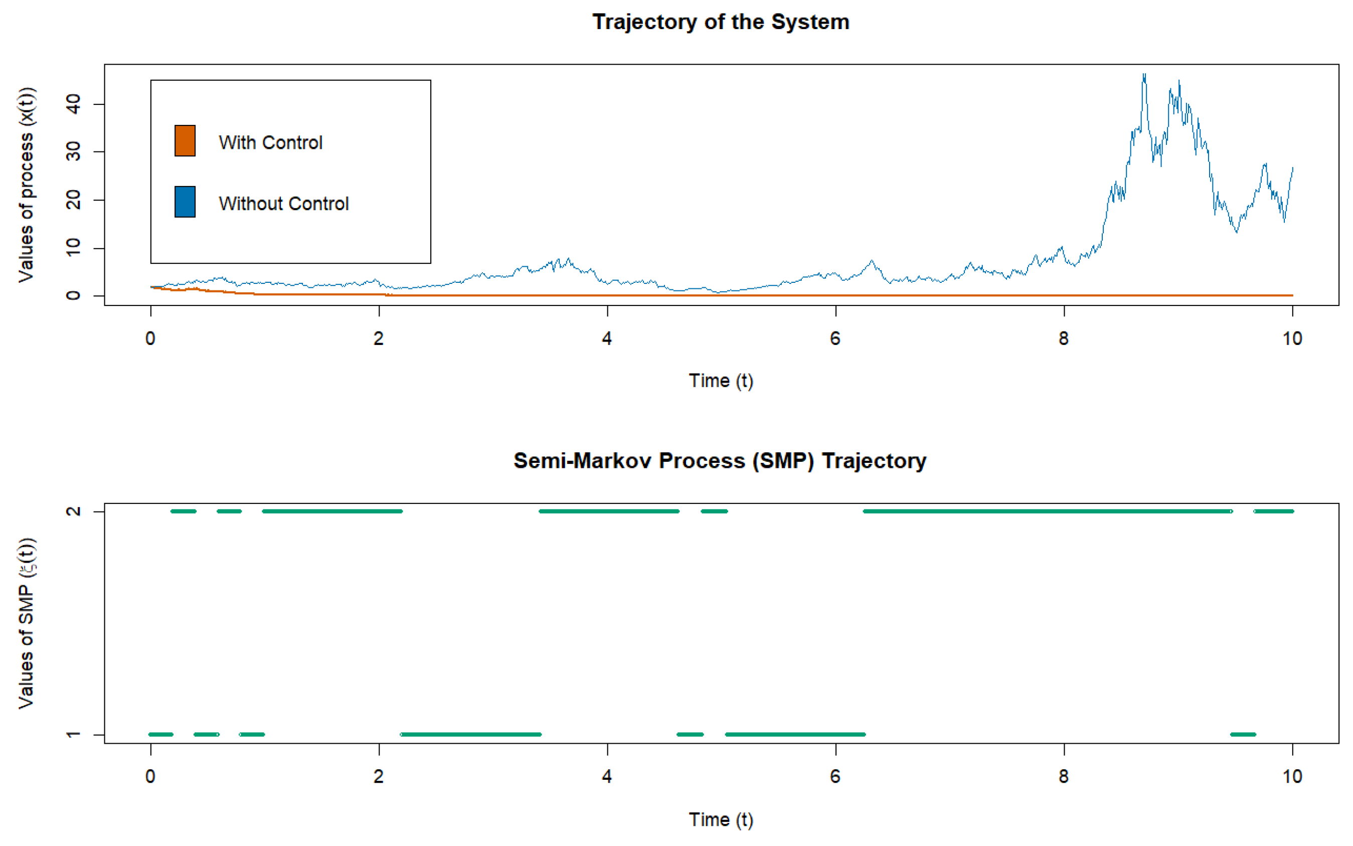
The optimal control is as follows

$$u_k^0(t,x;1)=-0.847x\left(t\right),u_k^0(t,x;2)=-0.397x\left(t\right).$$

(49)

Simulated trajectory of the solution (46) and (47) without control and under the influence of optimal control is shown in Figure 1.

8. Discussion

The main focus of this paper is on theoretical derivations of the optimal control system for stochastic differential equations in the presence of external perturbations described by semi-Markov processes. This generalization allows us to more accurately describe the dynamics of real processes under various restrictions on the spend time ${\theta }_n$ in states, which is impossible in the case of a Markov process. In Theorem 2, we find an explicit form of the infinitesimal operator, which is determined on the basis of the coefficients of the original equation and the characteristics of the semi-Markov process. This representation allows us to synthesize the optimal control $u^0(t,x)$ based on the Bellman equation (18) with the boundary condition (19). For the linear case of the system of the form (30), the search for optimal control is carried out on the basis of solving the Riccati equation (39), which also arises in the case of the presence of a Markovian external perturbation.

As we can see from Figure 1, the controlled solution visually resembles an asymptotically stable one, but from Figure 2 it is clear that the solution is not. Thus, asymptotic stability may not be achieved by constructing an optimal control. The problem of stability and stability of the solution will be the subject of research in subsequent articles.

The main focus in the following works for dynamical systems with semi-Markovian external perturbations will be on taking into account the ergodic properties of the semi-Markovian process $\xi \left(t\right),t\ge 0$ when analyzing the asymptotic behavior of the system. In contrast to systems with Markovian external switches, where the ergodic properties of $\xi \left(t\right)$ were described on the basis of intensities $\lambda \left(y\right)$, for the semi-Markovian case, conditions on the times of steady state and jumps will play an important role. Thus, the parameter estimate of model (2) will have not only an estimate of the parameters $a(·),b(·)$, but also an estimate of the distribution of the residence time in the states. Therefore, the following algorithm can be proposed for system analysis and parameter estimation:

• Estimation of switching moments

  $${\tau }_n=\sum _{i=1}^n{\theta }_n;$$
  This estimation can be realized using a generalized unit-root test developed for time series [22];
• Estimation state space for semi-Markov process $\xi \left(t\right)$,

  $$\mathbf{Y}=\{1,2,...,N\};$$
• Estimation coefficients $a(·),b(·)$ for SDE (2);

The presented framework of stochastic dynamic systems with semi-Markov parameters offers a promising tool for systems biology and systems medicine. In systems biology, it can help model complex molecular interactions, such as oxidative stress and mitochondrial dysfunction, influenced by stochastic perturbations. In systems medicine, this approach supports personalized treatment strategies by capturing patient-specific dynamics. For instance, it can predict disease progression and optimize therapies in conditions like Parkinson’s Disease. By integrating theoretical modeling with clinical data, this framework bridges the gap between understanding disease mechanisms and advancing precision medicine.

9. Conclusions

We propose optimal control strategies for stochastic dynamical systems with semi-Markov parameters. A linear optimization algorithm is derived and its convergence substantiated. This work focused primarily on the generalization of the Markov model, which would allow for a more accurate description of real processes in which switching occurs at random times, not subject to an exponential distribution. The developed theory currently has a number of advantages, but there are a variety of limitations to consider when interpreting the results. First, semi-Markov switching models require defining a distribution of switching times, which complicates estimation of model parameters. Second, the use of the semi-Markov process requires the verification of the finiteness of the necessary moments, and in the case of the Markov switching process, this verification was reduced to the inequality $0<{\lambda }_{min}<{\lambda }_{max}<\infty$, where ${\lambda }_{min},{\lambda }_{max}$—minimal and maximal intensity for the Markov switching process. Future work in this direction will develop algorithms for estimating optimal control for nonlinear systems with quadratic and quadratic-exponential performance functions.