Discrete-Time Dynamical Systems on Structured State Spaces: State-Transition Laws in Finite-Dimensional Lie Algebras

Abstract

The present paper elaborates on the development of a theory of discrete-time dynamical systems on finite-dimensional structured state spaces. Dynamical systems on structured state spaces possess well-known applications to solving differential equations in physics, and it was shown that discrete-time systems on finite- (albeit high-) dimensional structured state spaces possess solid applications to structured signal processing and nonlinear system identification, modeling and control. With reference to the state-space representation of dynamical systems, the present contribution tackles the core system-theoretic problem of determining suitable laws to express a system’s state transition. In particular, the present contribution aims at formulating a fairly general class of state-transition laws over the Lie algebra associated to a Lie group and at extending some properties of classical dynamical systems to process Lie-algebra-valued state signals.

1. Introduction

According to a widely deployed definition of a discrete-time signal, which emphasizes the role of its informational content, a signal is a time-varying function that carries on information about the features of some phenomena [1,2]. A signal is denoted as $k\mapsto x_k$, where $k\in \mathbb{Z}$ denotes a discrete index that distinguishes one sample of the signal x from another. The nature and meaning of the values $x_k$ may be arbitrary, and the information content conveyed by a signal emerges from the statistical distribution of the samples within a signal’s domain or from the temporal features of the signal. Likewise, a discrete-time system is any (no matter how abstract) set of components that takes an input signal (no matter how structured) and yields an output signal (not necessarily in the same domain).

In classical system theory [3,4], a signal takes values in an unstructured domain such as the real line $\mathbb{R}$ or in the multidimensional space ${\mathbb{R}}^n$, and the discrete-time system that processes this signal is designed to input, treat and output real-valued samples. Whenever the attributes of the phenomenon underlying the observed signal are subjected to any constraints, the signal takes values on a structured domain (the more complicated the constraints, the more structured the signals, the more involved the design of systems able to process such signals.) A category of dynamical systems possessing a structured state space is given by the class of graph dynamical systems [5]. Largely diffused are models of complex systems that take, as state spaces, curved manifolds (or state manifolds) as well as Lie groups [6,7,8,9,10].

A structured signal may be, for instance, a sequence of real-valued, positive numbers $x_k>0$ (such as a sequence of temperatures expressed by the Kelvin scale) or a complex-valued sequence $x_k\in \mathbb{C}$ [11], $k\in \mathbb{Z}$, or a quaternionic sequence [12]. A structured signal may also appear, for example, under the form of a sequence of square matrices whose entries obey mutual constraints. This is the case encountered in robotics and avionics [13] or in bio-mechanics [14]. From a practitioner standpoint, Lie-group theory provides powerful mathematical tools to perform computations and to design numerical algorithms on a “nonlinear” Lie group by means of linear tools on its associated Lie algebra.

Over the last decade, there has been a flourishing of contributions in system theory and control that evidenced how sequences of finite-dimensional Lie-algebra elements (namely, Lie-algebra signals) call for appropriate processing system design. An example is illustrated in the paper [9], whose authors developed a Kalman-like filtering algorithm on a group of symmetric, positive-definite matrices for objects tracking. Following early contributions to the theory of structured state-space system regulation [15], recent research efforts deepened its understanding and practice [16,17,18,19,20].

Aside from the remarkable, purely theoretical, contributions on the subject of Lie-algebra state-space system modeling and control [13,21,22,23,24,25], applications of structured state-space systems range from switched electrical networks [26] to quantum dynamics [27,28,29,30], from motion tracking and control [31,32,33,34] to bioengineering [35], and from machinery and structural engineering [36,37,38] to unconventional robotics and unmanned vehicle engineering [39,40].

The present contribution aims at extending some classical tools of linear system theory [3,4] to Lie-algebra systems. In particular, the present paper is organized as follows. Section 2 introduces Lie-algebra signals and discrete-time linear systems on finite-dimensional Lie algebras, both being considered as essential building blocks in a larger theory of Lie-group signals/systems. Section 3 lays out prominent features and properties of Lie-algebra signals and Lie-algebra dynamical systems. Then, Section 4 treats a special system as a case study and traces its structural properties. Finally, Section 5 concludes this paper and lays some future research directions.

2. Lie-Algebra Signals and Discrete-Time Linear Systems on Finite-Dimensional Lie Algebras

This section presents the main definitions, with the notations used in this paper presented in Section 2.1. In addition, Section 2.2 introduces the notion of discrete-time linear systems on finite-dimensional Lie algebras and the notion of Lie-algebra signals, as well as auxiliary mathematical tools such as the Z-transform, the discrete-time Fourier transform and the cross-correlation function of Lie-algebra signals.

2.1. Notation and Definitions

A Lie algebra is a vector space $\mathfrak{g}$ over some field $\mathbb{F}$, together with a binary operation $[·,·]:\mathfrak{g}\times \mathfrak{g}\to \mathfrak{g}$ called the Lie bracket, that satisfies the following axioms:

• Bilinearity: $[\alpha x+\beta y,z]=\alpha [x,z]+\beta [y,z]$, $[z,\alpha x+\beta y]=\alpha [z,x]+\beta [z,y]$ for all scalars $\alpha ,\beta \in \mathbb{F}$ and all elements $x,y,z\in \mathfrak{g}$.
• Alternativity: $[x,x]=0$ for all $x\in \mathfrak{g}$.
• The Jacobi identity: $[x,[y,z\left]\right]+[z,[x,y\left]\right]+[y,[z,x\left]\right]=0$ for all $x,y,z\in \mathfrak{g}$.

Upon using the property of bilinearity to expand the Lie bracket $[x+y,x+y]$ together with the property of alternativity leads to $[x,y]+[y,x]=0$ for all elements $x,y\in \mathfrak{g}$, showing that bilinearity and alternativity together imply the anticommutativity property, namely $[x,y]=-[y,x]$, for all elements $x,y\in \mathfrak{g}$.

The dimension of a Lie algebra is its dimension as a vector space over the field $\mathbb{F}$. The Lie bracket is not associative in general, meaning that $\left[\right[x,y],z]$ need not equal $[x,[y,z\left]\right]$. A subspace $\mathfrak{h}\subseteq \mathfrak{g}$ that is closed under the Lie bracket is called a Lie subalgebra.

Example 1.

As an example, take the following structured discrete-time signal:

$$X_k:=\left[\begin{array}{ccc}0& a_k& b_k\\ -a_k& 0& c_k\\ -b_k& -c_k& 0\end{array}\right],$$

with $a_k,b_k,c_k\in \mathbb{R}$ for any $k\in \mathbb{Z}$. Such a signal appears as a sequence $k\mapsto X_k$ of $3\times 3$ matrices, such that $X_k^T=-X_k$ for any $k\in \mathbb{Z}$, namely each matrix $X_k\in \mathfrak{so}\left(3\right)$, where $\mathfrak{so}\left(3\right)$ denotes the Lie algebra of all the $3\times 3$ skew-symmetric matrices. In this example, the entries of each matrix $X_k$ satisfy mutual linear constraints. By the Lie-group theory, it is known that skew-symmetric matrices like $X_k$ are precisely associated with the Lie group $\mathrm{SO}\left(3\right)$ of three-dimensional rotations.

The space $\mathfrak{so}\left(3\right)$ is apparently a linear space of dimension 3. The Lie bracket is defined as $[X,Y]:=XY-YX$, for every pair $X,Y\in \mathfrak{so}\left(3\right)$, and coincides with the commutator operator for matrices. When dealing with the dynamics of a rigid body, a $\mathfrak{so}\left(3\right)$-signal arises naturally from the evolution of the angular velocity matrix associated to the spatial attitude of the body (see, e.g., the example of a spacecraft [40]).

A homomorphism $f:\mathfrak{g}\to {\mathfrak{g}}^{\prime }$ between two Lie algebras (over the same base field) is a linear map that is compatible with the respective Lie brackets, namely $f\left({[x,y]}_{\mathfrak{g}}\right)={[f\left(x\right),f\left(y\right)]}_{{\mathfrak{g}}^{\prime }}$, for all elements $x,y\in \mathfrak{g}$.

Given two subsets ${\mathfrak{s}}_1\subset \mathfrak{g}$ and ${\mathfrak{s}}_2\subset \mathfrak{g}$ of a finite-dimensional Lie algebra $\mathfrak{g}$, their sum is defined as ${\mathfrak{s}}_1+{\mathfrak{s}}_2:=\{x+y | x\in {\mathfrak{s}}_1, y\in {\mathfrak{s}}_2\}$. Given a finite number of subsets ${\mathfrak{s}}_i\subset \mathfrak{g}$, their summation ${\mathfrak{s}}_1+{\mathfrak{s}}_2+\cdots$ is denoted by ${\sum }_i{\mathfrak{s}}_i$.

A finite-dimensional Lie algebra on the field $\mathbb{C}$ is a vector space that can be endowed with an inner product ${(·,·)}_{\mathfrak{g}}:\mathfrak{g}\times \mathfrak{g}\to \mathbb{C}$. The following distinguishing properties of the inner product are worth recalling: given any two elements $x,y\in \mathfrak{g}$ and any constant $c\in \mathbb{C}$, (1) it holds that ${(cx,y)}_{\mathfrak{g}}=c{(x,y)}_{\mathfrak{g}}$, which is termed linearity in the first argument; (2) it holds that ${(x,y)}_{\mathfrak{g}}={(y,x)}_{\mathfrak{g}}^{*}$, where the superscript $*$ denotes complex conjugation; and (3) it holds that ${(x,x)}_{\mathfrak{g}}\ge 0$ with equality only for $x=0$. The properties (1) and (2) imply that ${(x,cy)}_{\mathfrak{g}}=c^{*}{(x,y)}_{\mathfrak{g}}$. An inner product ${(·,·)}_{\mathfrak{g}}$ induces a norm ${\parallel ·\parallel }_{\mathfrak{g}}$, defined as ${\parallel x\parallel }_{\mathfrak{g}}^2:={(x,x)}_{\mathfrak{g}}$, for every $x\in \mathfrak{g}$.

Let ${\mathfrak{g}}^{\mathrm{s}}$ denote the set of sequences of elements of a Lie algebra $\mathfrak{g}$, namely $\mathbb{Z}\ni k\mapsto x_k\in \mathfrak{g}$. A Lie-algebra sequence in ${\mathfrak{g}}^{\mathrm{s}}$ is denoted by $x_{•}$.

Let $\mathrm{End}\left(\mathfrak{g}\right)$ denote the set of endomorphisms of $\mathfrak{g}$, namely, the set of all the $\mathbb{C}$-linear maps from the Lie algebra to itself. Given an endomorphism $\mathrm{a}\in \mathrm{End}\left(\mathfrak{g}\right)$ and an element $x\in \mathfrak{g}$, the application of the endomorphism to the element is denoted, in the present paper, by $\mathrm{a}\diamond x$. The notation $\mathrm{a}\diamond \mathfrak{g}$ refers to the set $\{\mathrm{a}\diamond x | x\in \mathfrak{g}\}$. The composition of endomorphisms is also denoted by the symbol ⋄, namely, given any two endomorphisms $\mathrm{a},\mathrm{b}\in \mathrm{End}\left(\mathfrak{g}\right)$, their composition is an endomorphism, i.e., $\mathrm{a}\diamond \mathrm{b}\in \mathrm{End}\left(\mathfrak{g}\right)$.

Example 2.

Below is a partial exemplary list of Lie-algebra endomorphisms:

• Identity endomorphism: It is denoted by ${\mathrm{id}}_{\mathfrak{g}}$ and is defined by ${\mathrm{id}}_{\mathfrak{g}}\diamond x=x$, for every $x\in \mathfrak{g}$.
• Scaling endomorphism: It is denoted by ${\mathrm{af}}_c$ and is defined by ${\mathrm{af}}_c=c{\mathrm{id}}_{\mathfrak{g}}$, for any given $c\in \mathbb{C}$.
• Inverse of an endomorphism: Given an endomorphism $\mathrm{a}\in \mathrm{End}\left(\mathfrak{g}\right)$, its inverse is denoted by ${\mathrm{a}}^{-1}$ and is such that ${\mathrm{a}}^{-1}\diamond \mathrm{a}=\mathrm{a}\diamond {\mathrm{a}}^{-1}={\mathrm{id}}_{\mathfrak{g}}$. The notion of inverse of an endomorphism may be generalized in several ways. For example, the g-inverse of an endomorphism $\mathrm{a}\in \mathrm{End}\left(\mathfrak{g}\right)$ is denoted by ${\mathrm{a}}^{-}\in \mathrm{End}\left(\mathfrak{g}\right)$ and is such that $\mathrm{a}\diamond {\mathrm{a}}^{-}\diamond \mathrm{a}=\mathrm{a}$ [41].
• Adjoint endomorphism: It is denoted by ${\mathrm{ad}}_v$ and is defined by ${\mathrm{ad}}_v\diamond x:=[v,x]$, for a given element $v\in \mathfrak{g}$. (In matrix Lie algebras, the Lie brackets coincide with the matrix commutator.)
• Adjoint of an endomorphism induced by the inner product structure. Given an element $\mathrm{a}\in \mathrm{End}\left(\mathfrak{g}\right)$, its adjoint with respect to the inner product is the unique element ${\mathrm{a}}^{†}\in \mathrm{End}\left(\mathfrak{g}\right)$ such that ${(\mathrm{a}\diamond x,y)}_{\mathfrak{g}}={(x,{\mathrm{a}}^{†}\diamond y)}_{\mathfrak{g}}$ for every $x,y\in \mathfrak{g}$. Given two endomorphisms $\mathrm{a},\mathrm{b}\in \mathrm{End}\left(\mathfrak{g}\right)$, it holds that ${(\mathrm{a}\diamond \mathrm{b})}^{†}={\mathrm{b}}^{†}\diamond {\mathrm{a}}^{†}$.
• Linear combination of endomorphisms: The $\mathbb{C}$-linear combination of two endomorphisms is a new endomorphism, namely, given two scalars $c_1,c_2\in \mathbb{C}$, it holds that $c_1\mathrm{a}+c_2\mathrm{b}\in \mathrm{End}\left(\mathfrak{g}\right)$. In fact, the space $\mathrm{End}\left(\mathfrak{g}\right)$ is closed under multiplication by a complex-valued constant and under addition.

Since every Lie-algebra endomorphism is a homomorphism of the Lie algebra to itself, every endomorphism preserves the Lie brackets, namely $\mathrm{a}\diamond [u,v]=[\mathrm{a}\diamond u,\mathrm{a}\diamond v]$, for every $\mathrm{a}\in \mathrm{End}\left(\mathfrak{g}\right)$ and $u,v\in \mathfrak{g}$.

The algebraic structure $\left(\mathrm{End}\right(\mathfrak{g}),\diamond ,+)$ is a unital algebraic ring, where the ring multiplication is $\mathrm{a}\diamond \mathrm{b}\in \mathrm{End}\left(\mathfrak{g}\right)$, the ring identity is ${\mathrm{id}}_{\mathfrak{g}}$ and the ring addition is $\mathrm{a}+\mathrm{b}$ for every $\mathrm{a},\mathrm{b}\in \mathrm{End}\left(\mathfrak{g}\right)$. The set $\mathrm{End}\left(\mathfrak{g}\right)$ is an Abelian group under addition; the group multiplication ⋄ is associative and distributive over the group addition +.

The present paper also deals with sequences of endomorphisms. One such sequence is denoted by ${\mathrm{a}}_{•}$, whereas the symbol ${\mathrm{a}}_k$ denotes the $k^{\mathrm{th}}$ element of a sequence ${\mathrm{a}}_{•}$, with $k\in \mathbb{Z}$. The space of the sequences of endomorphisms in $\mathrm{End}\left(\mathfrak{g}\right)$ is denoted as ${\mathrm{End}}^{\mathrm{s}}\left(\mathfrak{g}\right)$. The unit impulse sequence is denoted as ${\mathrm{d}}_{•}\in {\mathrm{End}}^{\mathrm{s}}\left(\mathfrak{g}\right)$ and is defined by

$${\mathrm{d}}_k:=\left\{\begin{array}{ccc}{\mathrm{id}}_{\mathfrak{g}}\hfill & if& k=0,\hfill \\ {\mathrm{af}}_0\hfill & if& k\ne 0.\hfill \end{array}\right.$$

(1)

The convolution operator between sequences of endomorphisms and its inverse operation are defined as follows.

Definition 1.

Given two sequences of endomorphisms ${\mathrm{g}}_{•},{\mathrm{h}}_{•}\in {\mathrm{End}}^{\mathrm{s}}\left(\mathfrak{g}\right)$, their convolution is defined as ${({\mathrm{g}}_{•}\otimes {\mathrm{h}}_{•})}_k:={\sum }_i{\mathrm{g}}_i\diamond {\mathrm{h}}_{k-i}$. The convolution produces a sequence of endomorphisms, namely, ${\mathrm{g}}_{•}\otimes {\mathrm{h}}_{•}\in {\mathrm{End}}^{\mathrm{s}}\left(\mathfrak{g}\right)$. The inverse operation is termed deconvolution. The deconvolution of a sequence ${\mathrm{g}}_{•}\in {\mathrm{End}}^{\mathrm{s}}\left(\mathfrak{g}\right)$ is denoted as ${\mathrm{g}}_{•}^{\Delta }\in {\mathrm{End}}^{\mathrm{s}}\left(\mathfrak{g}\right)$ and is defined by ${\mathrm{g}}_{•}\otimes {\mathrm{g}}_{•}^{\Delta }={\mathrm{g}}_{•}^{\Delta }\otimes {\mathrm{g}}_{•}={\mathrm{d}}_{•}$.

Even the structure $({\mathrm{End}}^{\mathrm{s}}\left(\mathfrak{g}\right),\otimes ,+)$ is a unital algebraic ring. The ring multiplication is ${\mathrm{a}}_{•}\otimes {\mathrm{b}}_{•}\in {\mathrm{End}}^{\mathrm{s}}\left(\mathfrak{g}\right)$, the ring identity is the unit impulse sequence ${\mathrm{d}}_{•}\in {\mathrm{End}}^{\mathrm{s}}\left(\mathfrak{g}\right)$, while the ring addition is ${\mathrm{a}}_{•}+{\mathrm{b}}_{•}$, for every ${\mathrm{a}}_{•},{\mathrm{b}}_{•}\in {\mathrm{End}}^{\mathrm{s}}\left(\mathfrak{g}\right)$. The set ${\mathrm{End}}^{\mathrm{s}}\left(\mathfrak{g}\right)$ is an Abelian group under addition; the multiplication ⊗ is associative as well as distributive over the addition.

2.2. Finite-Dimensional Lie-Algebra Signals and Lie-Algebra Linear Systems

In system theory, a discrete-time dynamical system is typically represented in either the input–output form or in the input–state–output form [3]. The representation considered in the present subsection only involves the input and the state signals, while the output signal and the subsystem that transforms the state into the output are hidden.

An example of finite-dimensional Lie-algebra system is recalled below.

Example 3.

Let us consider Brockett’s “double bracket” dynamical system discussed in [42]. Its discrete-time version reads

$$H_k=H_{k-1}+[H_{k-1},[N,H_{k-1}]],$$

where $H_k$ denotes a sequence of symmetric matrices of finite, although arbitrary, dimension, the Lie bracket denotes matrix commutator and N denotes a fixed symmetric matrix. The space of symmetric matrices is clearly a linear space under standard matrix operations, and, when endowed with a pair of Lie brackets, it forms a Lie algebra.

As it is apparent from the above example, iterated Lie brackets are encountered in Lie-algebra dynamical systems. It is therefore of use to recall the following definition that helps in characterizing a class of systems known as nilpotent.

Definition 2.

Let $\mathfrak{h}$ denote a subset of $\mathfrak{g}$. The set of elements $x\in \mathfrak{g}$ such that $[x,s]=0$ for all $s\in \mathfrak{h}$ forms a subalgebra called the centralizer of $\mathfrak{h}$. The centralizer of a Lie algebra itself is called its center. Similarly, if $\mathfrak{h}$ is a subspace of a Lie algebra $\mathfrak{g}$, then the set of elements $x\in \mathfrak{g}$ such that $[x,s]\in \mathfrak{h}$ for all $s\in \mathfrak{h}$ forms a subalgebra called the normalizer of $\mathfrak{h}$. More generally, a Lie algebra $\mathfrak{g}$ is nilpotent if the succession

$$\mathfrak{g}, [\mathfrak{g},\mathfrak{g}], \left[\right[\mathfrak{g},\mathfrak{g}],\mathfrak{g}], \left[\right[[\mathfrak{g},\mathfrak{g}],\mathfrak{g}],\mathfrak{g}], \dots$$

eventually becomes zero.

A class of finite-dimensional Lie algebra dynamical systems is defined as follows.

Definition 3.

A discrete-time, linear, time-invariant system on a finite-dimensional Lie algebra $\mathfrak{g}$, denoted by LA·LTI ($p,q$) is defined by the following recursive scheme:

$$x_k=\sum _{i=1}^p{\mathrm{a}}_i\diamond x_{k-i}+\sum _{j=0}^q{\mathrm{b}}_j\diamond u_{k-j},$$

(2)

where the symbol $k\in \mathbb{Z}$ denotes a discrete-time index; the discrete-time sequence $x_{•}\in {\mathfrak{g}}^{\mathrm{s}}$ denotes the state of the LA·LTI system; the discrete-time sequence $u_{•}\in {\mathfrak{g}}^{\mathrm{s}}$ denotes the input of the LA·LTI system; the ${\mathrm{a}}_i,{\mathrm{b}}_i$ are elements of $\mathrm{End}\left(\mathfrak{g}\right)$; the term ${\sum }_{i=1}^p{\mathrm{a}}_i\diamond x_{k-i}$ is called the autoregressive part of the LA·LTI model, where the finite integer p is the order of the autoregressive part; and the term ${\sum }_{j=0}^q{\mathrm{b}}_i\diamond u_{k-j}$ is called the moving-average part of the LA·LTI model, where the finite integer q is the order of the moving average part.

In classical system theory, the input space and the state space do not need to be coincident [3]. Such a choice could also be implemented in the present context, but most of the notation would change to a more complicated one (for example, the operator $\mathrm{b}$ will not be a $\mathfrak{g}$-endomorphism any longer). To solve this problem, that arises, for example, in Lie-group signal filtering (see, e.g., the camera-tracking problem tackled in [43]), it is necessary to add a further equation that transforms the Lie-group input signal into a Lie-algebra input signal $u_k$. The full system equations, involving the Lie-group input and output sequences as well as the Lie-algebra input and state sequences, are currently under investigation and will be presented in a forthcoming contribution.

The fundamental, structural linearity and time-invariance properties of the dynamical system (2) may be expressed as follows.

Property 1.

The system (2) is linear and time-invariant. In fact, the response of the superposition of two input sequences $u_{•}^{\prime }\in {\mathfrak{g}}^{\mathrm{s}}$ and $u_{•}^{″}\in {\mathfrak{g}}^{\mathrm{s}}$ is the superposition of the two responses, because ${\mathrm{h}}_{•}\otimes (u_{•}^{\prime }+u_{•}^{″})={\mathrm{h}}_{•}\otimes u_{•}^{\prime }+{\mathrm{h}}_{•}\otimes u_{•}^{″}$, for any ${\mathrm{h}}_{•}\in {\mathrm{End}}^{\mathrm{s}}\left(\mathfrak{g}\right)$. Moreover, for any ${\mathrm{h}}_{•}\in {\mathrm{End}}^{\mathrm{s}}\left(\mathfrak{g}\right)$ and $u_{•}\in {\mathfrak{g}}^{\mathrm{s}}$, the response of an input sequence shifted by a fixed lag $n\in \mathbb{Z}$, namely $u_{•+n}\in {\mathfrak{g}}^{\mathrm{s}}$, is the shifted response to the un-shifted input, because ${\mathrm{h}}_{•}\otimes u_{•+n}=x_{•+n}$, where $x_{•}:={\mathrm{h}}_{•}\otimes u_{•}$.

A fundamental mathematical tool to design and analyze discrete-time, linear and time-invariant dynamical systems is the Z-transform of Lie-algebra sequences.

Definition 4.

Let $\mathfrak{g}$ denote a finite-dimensional Lie algebra on the field of complex numbers $\mathbb{C}$. The Z-transform operator${\mathcal{Z}}_{\mathfrak{g}}:{\mathfrak{g}}^{\mathrm{s}}\times \mathbb{C}\to \mathfrak{g}$ on the Lie algebra $\mathfrak{g}$ is defined as

$${\mathcal{Z}}_{\mathfrak{g}}\left\{x_{•}\right\}\left(z\right):=\sum _{k\in \mathbb{Z}}{x}_k{z}^{-k},$$

(3)

where $x_{•}\in {\mathfrak{g}}^{\mathrm{s}}$ and $z\in \mathbb{C}$ is a variable. The region of convergence (ROC) of the Z-transform of a sequence $x_{•}$ is defined as the maximal subset of the complex plane where the series (3) converges to a finite value, namely

$${\mathrm{ROC}}_x:=\left\{z\in \mathbb{C}\left|{∥\sum _k{x}_k{z}^{-k}∥}_{\mathfrak{g}}<+\infty \right.\right\}.$$

(4)

The ROC of any given sequence exhibits an annular shape, because it is of the form $\mathrm{ROC}=\{z\in \mathbb{C} | R_1\le | z | \le R_2\}$. An ROC includes the unit circle of the complex plane only if $R_1\le 1$ and $R_2\ge 1$. The Z-transform on a finite-dimensional Lie algebra over the field $\mathbb{C}$ is a $\mathbb{C}$-linear operator.

In the present context, it is necessary to define a similar operator applicable to sequences of endomorphisms.

Definition 5.

Given a sequence ${\mathrm{h}}_{•}\in {\mathrm{End}}^{\mathrm{s}}\left(\mathfrak{g}\right)$, its Z-transform ${\mathcal{Z}}_{\mathrm{End}\left(\mathfrak{g}\right)}:{\mathrm{End}}^{\mathrm{s}}\left(\mathfrak{g}\right)\times \mathbb{C}\to \mathrm{End}\left(\mathfrak{g}\right)$ is defined as

$${\mathcal{Z}}_{\mathrm{End}\left(\mathfrak{g}\right)}\left\{{\mathrm{h}}_{•}\right\}\left(z\right):=\sum _{k\in \mathbb{Z}}{\mathrm{h}}_k{z}^{-k},$$

(5)

where $z\in \mathbb{C}$ is a variable and, since the space $\mathrm{End}\left(\mathfrak{g}\right)$ is closed under addition and multiplication by a complex-valued scalar, ${\mathcal{Z}}_{\mathrm{End}\left(\mathfrak{g}\right)}\left\{{\mathrm{h}}_{•}\right\}\left(z\right)$, for any fixed value of z, is an element of $\mathrm{End}\left(\mathfrak{g}\right)$.

Prominent properties of the Z-transform of a Lie-algebra-valued sequence and of a Lie-algebra endomorphism sequence are laid out as follows.

Property 2.

The Z-transform on a Lie-algebra enjoys the following important properties:

Time-delay formula: The The Z-transform of a delayed sequence obeys the rule ${\mathcal{Z}}_{\mathfrak{g}}\left\{x_{•-n}\right\}\left(z\right)={\mathcal{Z}}_{\mathfrak{g}}\left\{x_{•}\right\}\left(z\right)z^{-n}$, for every Lie-algebra sequence $x_{•}\in {\mathfrak{g}}^s$ and any lag $n\in \mathbb{Z}$.

Time/Z-domain duality: The Z-transform of a convolution of endomorphism sequences obeys the rule ${\mathcal{Z}}_{\mathrm{End}\left(\mathfrak{g}\right)}\{{\mathrm{h}}_{•}\otimes {\mathrm{g}}_{•}\}\left(z\right)={\mathcal{Z}}_{\mathrm{End}\left(\mathfrak{g}\right)}\left\{{\mathrm{g}}_{•}\right\}\left(z\right)\diamond {\mathcal{Z}}_{\mathrm{End}\left(\mathfrak{g}\right)}\left\{{\mathrm{h}}_{•}\right\}\left(z\right)$, for every ${\mathrm{h}}_{•},{\mathrm{g}}_{•}\in {\mathrm{End}}^{\mathrm{s}}\left(\mathfrak{g}\right)$.

In order to define a measure of similarity of two Lie-algebra sequences, building on the classical system theory, we define their cross-correlation function as follows.

Definition 6.

Given two sequences $x_{•},y_{•}$ in ${\mathfrak{g}}^{\mathrm{s}}$, their complex-valued cross-correlation function is defined as

$$R_{xy}(m,n):=\sum _k{(x_{k+m},y_{k+n})}_{\mathfrak{g}},$$

(6)

where the integers $m,n\in \mathbb{Z}$ are termed lags at which the cross-correlation is evaluated. It holds that $R_{yx}(n,m)=R_{xy}^{*}(m,n)$. The autocorrelation function associated to a sequence $x_{•}\in {\mathfrak{g}}^{\mathrm{s}}$ is denoted by $R_{xx}(m,n)$ and measures the temporal self-similarity of a sequence. If the function $R_{xx}(m,n)$ is constant for every pair $m,n$ such that $m-n$ is constant (namely, the matrix representation of the autocorrelation $R_{xx}$ is Toepliz), then the autocorrelation is specified by its first row (or column) and is denoted by $R_{xx}\left(n\right):={\sum }_k{(x_k,x_{k+n})}_{\mathfrak{g}}$. The quantity $R_{xx}\left(0\right)={\sum }_k{\parallel x_k\parallel }_{\mathfrak{g}}^2$ is termed energy of the sequence $x_{•}$ and is clearly real-valued and non-negative.

If a sequence has nonzero finite energy, its autocorrelation coefficients may be defined as

$${\rho }_{xx}\left(n\right):={\displaystyle \frac{R_{xx}\left(n\right)}{R_{xx}\left(0\right)}}\in \mathbb{C}.$$

(7)

Since $| R_{xx}\left(n\right) | \le R_{xx}\left(0\right)$, for every n, the autocorrelation coefficients lay within the unit disk of $\mathbb{C}$ (border included). Also, it holds that $R_{xx}(-n)=R_{xx}^{*}\left(n\right)$. A sequence $x_{•}\in {\mathfrak{g}}^{\mathrm{s}}$ is termed uncorrelated if $R_{xx}\left(n\right)=0$ for every lag $n\ne 0$.

3. Structural Properties of the LA·LTI System

The present section aims to illustrate prominent structural properties of the LA·LTI system (2). Such properties are expressed intrinsically (or in coordinate-free fashion), without recurring to any specific choice of a basis of the Lie algebra $\mathfrak{g}$.

Section 3.1 defines and comments on properties such as the system transfer endomorphism, a counterpart of the system transfer function of classical system theory [3,4], along with its zeros and poles, and its associated impulse response endomorphism sequence. Section 3.2 introduces structural notions such as the properties of interconnected LA·LTI systems, the bounded-input/bounded-state stability and the property of causality. Section 3.3 studies the properties of the autocorrelation and of the cross-correlation functions of state sequences of LA·LTI systems along with their spectra.

3.1. System Transfer Endomorphism, Zeros, Poles and Impulse Response

Applying the Z-transform to both sides of the LA·LTI Equation (2) yields

$${\mathcal{Z}}_{\mathfrak{g}}\left\{x_{•}\right\}=\sum _{i=1}^p{\mathcal{Z}}_{\mathfrak{g}}\{{\mathrm{a}}_i\diamond x_{•-i}\}+\sum _{j=0}^q{\mathcal{Z}}_{\mathfrak{g}}\{{\mathrm{b}}_j\diamond u_{•-j}\}.$$

The endomorphisms ${\mathrm{a}}_i$ and ${\mathrm{b}}_i$ commute with the Z-transform; therefore,

$${\mathcal{Z}}_{\mathfrak{g}}\left\{x_{•}\right\}=\sum _{i=1}^p{\mathrm{a}}_i\diamond {\mathcal{Z}}_{\mathfrak{g}}\left\{x_{•-i}\right\}+\sum _{j=0}^q{\mathrm{b}}_j\diamond {\mathcal{Z}}_{\mathfrak{g}}\left\{u_{•-j}\right\}.$$

By using the time-delay property of the Z-transform (cf. Property 2) and upon defining the functions $X,U:\mathbb{C}\to \mathfrak{g}$ as

$$X\left(z\right):={\mathcal{Z}}_{\mathfrak{g}}\left\{x_{•}\right\}\left(z\right), U\left(z\right):={\mathcal{Z}}_{\mathfrak{g}}\left\{u_{•}\right\}\left(z\right),$$

(8)

the input–state relationship in the z-domain may be written as

$$\begin{array}{ccc}\hfill X\left(z\right)& =& \sum _{i=1}^p{\mathrm{a}}_i\diamond \left(X\left(z\right)z^{-i}\right)+\sum _{j=0}^q{\mathrm{b}}_j\diamond \left(U\left(z\right)z^{-j}\right),\hfill \\ & =& \left(\sum _{i=1}^p{z}^{-i}{\mathrm{a}}_i\right)\diamond X\left(z\right)+\left(\sum _{j=0}^q{z}^{-j}{\mathrm{b}}_j\right)\diamond U\left(z\right).\hfill \end{array}$$

It is convenient to define the two characteristic endomorphisms $\mathrm{A}\left(z\right),\mathrm{B}\left(z\right)\in \mathrm{End}\left(\mathfrak{g}\right)$ (for any fixed $z\in \mathbb{C}$) as

$$\mathrm{A}\left(z\right):=\sum _{i=1}^p{\mathrm{a}}_i{z}^{-i}, \mathrm{B}\left(z\right):=\sum _{j=0}^q{\mathrm{b}}_j{z}^{-j}.$$

(9)

Hence, the input–state relationship in the z-domain becomes

$$X\left(z\right)=\mathrm{A}\left(z\right)\diamond X\left(z\right)+\mathrm{B}\left(z\right)\diamond U\left(z\right).$$

(10)

The endomorphisms $\mathrm{A}\left(z\right)$ and $\mathrm{B}\left(z\right)$ are polynomials in the complex-valued variable $z^{-1}$ (with coefficients in $\mathrm{End}\left(\mathfrak{g}\right)$).

Property 3.

The transformed state-transition law (10) may be written in a way that resembles the familiar transfer-function representation in the z-domain, namely

$$X\left(z\right)=\mathrm{H}\left(z\right)\diamond U\left(z\right),$$

(11)

upon defining the quantity

$$\mathrm{H}(z):={({\mathrm{id}}_{\mathfrak{g}}-\mathrm{A}(z\left)\right)}^{-1}\diamond \mathrm{B}\left(z\right).$$

(12)

Since $\mathrm{A}\left(z\right)$ is a linear map, then ${({\mathrm{id}}_{\mathfrak{g}}-\mathrm{A}(z\left)\right)}^{-1}$ is also a linear map; therefore, $\mathrm{H}\left(z\right)\in \mathrm{End}\left(\mathfrak{g}\right)$ is termed system transfer endomorphism. Moreover, the system transfer endomorphism is a rational function of the complex-valued variable z.

The relationship (11) represents a fundamental result in system theory. The system transfer endomorphism models the system state for each possible input. Whenever the input sequence is provided, and its Z-transform is available in closed form, the state sequence may be computed by inverse-transforming the product (11). Moreover, the system transfer endomorphism summarizes a number of relevant information about an LTI system relative to its input-to-state relationship.

The notions of zeros and poles of the system transfer endomorphism of an LA·LTI system may be recovered by appropriate definitions.

Definition 7.

A value $z\in \mathbb{C}$ is termed a zero of an LA·LTI system if it is a root of the polynomial $\mathrm{B}\left(z\right)$, in addition to the eventual zeros at the origin. A value $z\in \mathbb{C}$ is termed the pole of an LA·LTI system if it makes the endomorphism ${\mathrm{id}}_{\mathfrak{g}}-\mathrm{A}\left(z\right)$ become singular.

The suggestive notation $det({\mathrm{id}}_{\mathfrak{g}}-\mathrm{A}(z))=0$ may be used to express the singularity of the endomorphism ${\mathrm{id}}_{\mathfrak{g}}-\mathrm{A}\left(z\right)$.

The notion of system impulse response may be recovered as well from the classical theory of linear time-invariant systems [3]. In fact, since the system transfer endomorphism $\mathrm{H}\left(z\right)$ is a rational function of the complex-valued variable z, it may be expanded in a Laurent-like [44] series:

$$\mathrm{H}(z)=\sum _i{\mathrm{h}}_i{z}^{-i},$$

(13)

where the endomorphisms ${\mathrm{h}}_i\in \mathrm{End}\left(\mathfrak{g}\right)$ play the role of coefficients of the system impulse response $h_{•}\in {\mathrm{End}}^{\mathrm{s}}\left(\mathfrak{g}\right)$. The input sequence $u_{•}\in \mathfrak{g}$, the state sequence $x_{•}\in \mathfrak{g}$ and the system impulse response endomorphisms of an LA·LTI system may be related by a convolution operation. Substituting the relationship (13) in Equation (11) yields

$$\sum _k{x}_k{z}^{-k}=\left(\sum _i{\mathrm{h}}_i{z}^{-i}\right)\diamond \left(\sum _j{u}_j{z}^{-j}\right)=\sum _j\sum _i{\mathrm{h}}_i\diamond u_j{z}^{-j-i}.$$

Applying the variable change $j=k-i$ in the double sum on the right-hand side gives

$$\sum _k{x}_k{z}^{-k}=\sum _k\sum _i{\mathrm{h}}_i\diamond u_{k-i}{z}^{-k}.$$

Hence, the input sequence, the state sequence and the system impulse response sequence relate by

$$x_{•}={\mathrm{h}}_{•}\otimes u_{•}:=\sum _i{\mathrm{h}}_i\diamond u_{•-i}.$$

(14)

The name “impulse response” is retained for convenience of description. It does not seem to possess an interpretation as the “response to an impulse” as it does in the classical theory of LA·LTI systems [3]. In addition, note that the convolution between a sequence of endomorphisms and a sequence of Lie-algebra elements has been denoted again with the symbol ⊗. Although one such choice is apparently a slight abuse of notation, it does not cause any confusion.

In the case that the ROC of the system transfer endomorphism $\mathrm{H}\left(z\right)$ includes the unit circle of the complex plane, the quantity $\mathrm{H}\left(e^{j\omega }\right)$ may be evaluated, where j denotes the imaginary unit and $\omega \in [0, 2\pi )$ is termed angular frequency. The quantity $\mathrm{H}\left(e^{j\omega }\right)$, for any fixed value of the angular frequency $\omega$, is termed the system frequency response endomorphism.

3.2. Canonical Interconnections of Systems, “bibs” Stability and Causality

The classical interconnection schemes [3], namely the cascade connection, the parallel connection and the feedback connection, may be extended to LA·LTI systems as explained in the following. The properties of these connections arise, substantially, by the property of the algebraic structure $({\mathrm{End}}^{\mathrm{s}}\left(\mathfrak{g}\right),\otimes ,+)$ to be a unital ring.

Definition 8.

The principal interconnections of LA·LTI systems are individuated as follows:

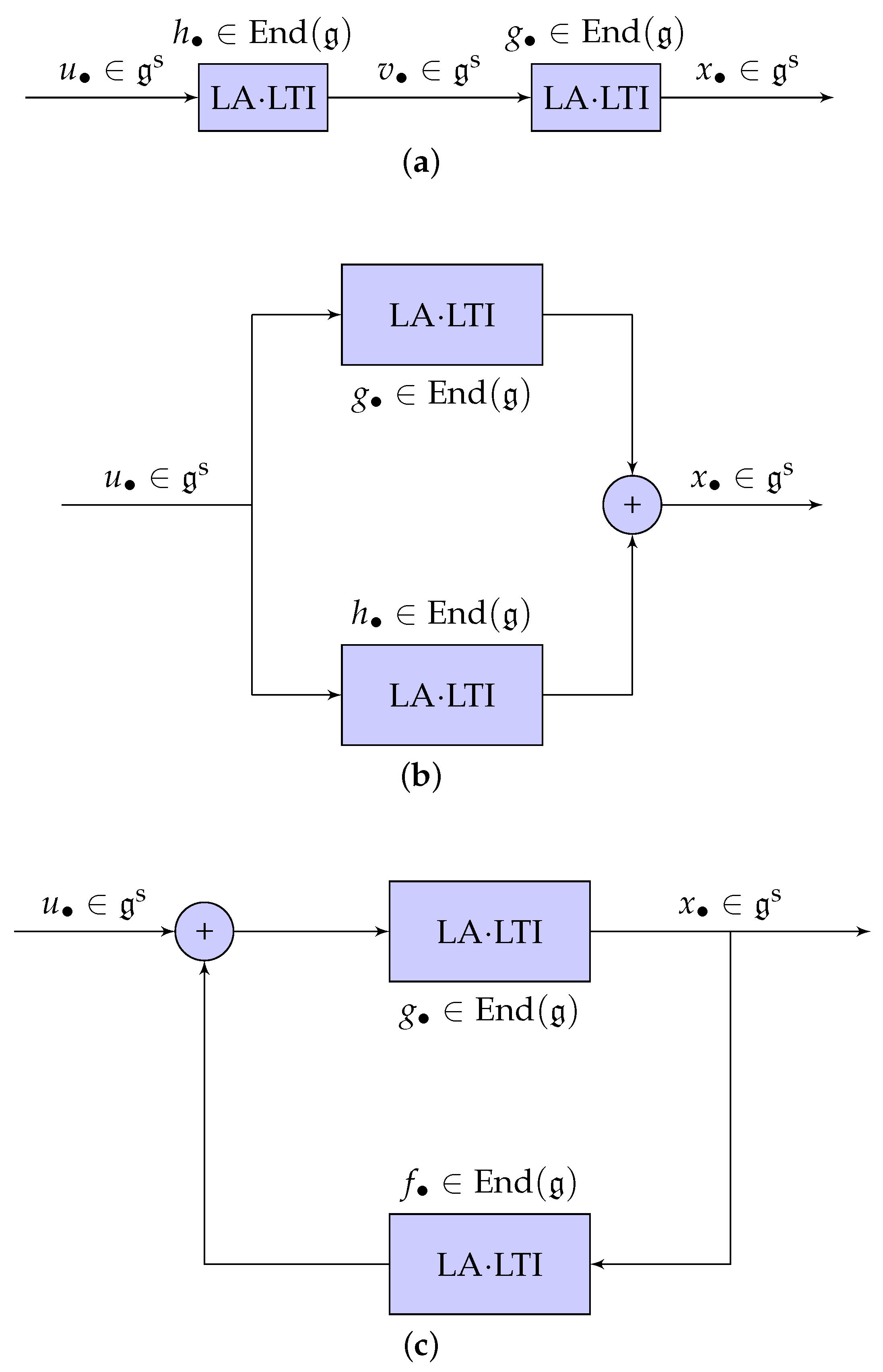
• Cascade connection: Given two LA·LTI subsystems with impulse responses ${\mathrm{h}}_{•}$ and ${\mathrm{g}}_{•}$, their cascade connection, presented in Figure 1a, is an LA·LTI system with impulse response ${\mathrm{g}}_{•}\otimes {\mathrm{h}}_{•}$. The system transfer endomorphism of a cascade is given by $\mathrm{G}\left(z\right)\diamond \mathrm{H}\left(z\right)$.
• Parallel connection: Given two LA·LTI subsystems with impulse responses ${\mathrm{h}}_{•}$ and ${\mathrm{g}}_{•}$, their parallel connection, presented in Figure 1b, is an LA·LTI system with impulse response ${\mathrm{g}}_{•}+{\mathrm{h}}_{•}$.The system transfer endomorphism of a parallel connection is given by $\mathrm{G}\left(z\right)+\mathrm{H}\left(z\right)$.
• Feedback connection: Given two LA·LTI subsystems with impulse responses ${\mathrm{g}}_{•}$ and ${\mathrm{f}}_{•}$, their feedback connection, presented in Figure 1c, is an LA·LTI system with impulse response ${({\mathrm{d}}_{•}-{\mathrm{g}}_{•}\otimes {\mathrm{f}}_{•})}^{\Delta }\otimes {\mathrm{g}}_{•}$. In fact, the overall state sequence is related with the overall input sequence by $x_{•}={\mathrm{g}}_{•}\otimes (u_{•}+{\mathrm{f}}_{•}\otimes x_{•})$. The system transfer endomorphism of a feedback connection is given by ${({\mathrm{id}}_{\mathfrak{g}}-\mathrm{G}(z)\diamond \mathrm{F}(z\left)\right)}^{-1}\diamond \mathrm{G}(z)$.

The feedback connection is a typical control structure for the direct system with impulse response ${\mathrm{g}}_{•}$. Whenever the input sequence of a feedback system is identicallyzero and the system is unstable, it may be used as an autonomous oscillator. This theory is known under the name of the Barkhausen oscillation criterion (see, e.g., [45]), which, in the present case, could be formulated in terms of the roots of the quantity $det({\mathrm{id}}_{\mathfrak{g}}-\mathrm{G}(z)\diamond \mathrm{F}(z\left)\right)$.

Define the norm of an endomorphism $\mathrm{a}\in \mathrm{End}\left(\mathfrak{g}\right)$ as follows:

$${\parallel \mathrm{a}\parallel }_{\mathrm{End}\left(\mathfrak{g}\right)}:=\underset{x\in \mathfrak{g}}{sup}\left\{{\displaystyle \frac{{\parallel \mathrm{a}\diamond x\parallel }_{\mathfrak{g}}}{{\parallel x\parallel }_{\mathfrak{g}}}}\right\}.$$

(15)

It holds that ${\parallel \mathrm{a}\diamond x\parallel }_{\mathfrak{g}}\le {\parallel \mathrm{a}\parallel }_{\mathrm{End}\left(\mathfrak{g}\right)}{\parallel x\parallel }_{\mathfrak{g}}$ for every $x\in \mathfrak{g}$. On the basis of the definition (15), one may recover the notion of bounded-input/bounded-state stability as follows.

Definition 9.

The LA·LTI system (2) is bounded-input/bounded-state (bibs)-stable provided that the energy ${\sum }_i{\parallel {\mathrm{h}}_i\parallel }_{\mathrm{End}\left(\mathfrak{g}\right)}$ of its impulse response is bounded. In fact, assume that the input sequence $u_k$ is bounded, namely that there exists a finite scalar $\overline{u}\ge 0$ such that $\parallel u_k{\parallel }_{\mathfrak{g}}\le \overline{u}$ for every k. Then,

$${\parallel x_k\parallel }_{\mathfrak{g}}={∥\sum _i{\mathrm{h}}_i\diamond u_{k-i}∥}_{\mathfrak{g}}\le \overline{u}\sum _i{\parallel {\mathrm{h}}_i\parallel }_{\mathrm{End}\left(\mathfrak{g}\right)}.$$

Likewise, it is quite straightforward to recover the notion of a causal LA·LTI system, as shown in the following definition.

Definition 10.

If the impulse response endomorphisms of an LA·LTI system are such that ${\mathrm{h}}_k={\mathrm{af}}_0$ for every $k<0$, the LA·LTI system is termed causal. In this case, in fact, the state $x_k$ depends only on the past values (as well as on the current value) of the input.

Figure 1. Lie-algebra input–state interconnection schemes of LA·LTI systems. (a) Cascade connection. The sequence $u_{•}$ denotes the overall input, the sequence $v_{•}$ denotes the intermediate state and the sequence $x_{•}$ denotes the overall state. (b) Parallel conenction. The sequence $u_{•}$ denotes the overall input and the sequence $x_{•}$ denotes the overall state. (c) Feedback connection. The sequence $u_{•}$ denotes the overall input and the sequence $x_{•}$ denotes the overall state. The LA·LTI system with impulse response ${\mathrm{f}}_{•}$ is a state feedback for the direct LA·LTI system with impulse response ${\mathrm{g}}_{•}$.

Figure 1. Lie-algebra input–state interconnection schemes of LA·LTI systems. (a) Cascade connection. The sequence $u_{•}$ denotes the overall input, the sequence $v_{•}$ denotes the intermediate state and the sequence $x_{•}$ denotes the overall state. (b) Parallel conenction. The sequence $u_{•}$ denotes the overall input and the sequence $x_{•}$ denotes the overall state. (c) Feedback connection. The sequence $u_{•}$ denotes the overall input and the sequence $x_{•}$ denotes the overall state. The LA·LTI system with impulse response ${\mathrm{f}}_{•}$ is a state feedback for the direct LA·LTI system with impulse response ${\mathrm{g}}_{•}$.

3.3. Correlation Functions and Power Spectra

The autocorrelation function $R_{xx}(m,n)$ of the state sequence of an LA·LTI system may be represented by $R_{xx}(m-n,0)=R_{xx}(m-n)$. In fact,

$$\begin{array}{cc}& R_{xx}(m,n)={\sum }_k{(x_{k+m},x_{k+n})}_{\mathfrak{g}}=\\ & {\sum }_k{\left({\sum }_{i=1}^p{\mathrm{a}}_i\diamond x_{k-i+m}+{\sum }_{j=0}^q{\mathrm{b}}_j\diamond u_{k-j+m},{\sum }_{i=1}^p{\mathrm{a}}_i\diamond x_{k-i+n}+{\sum }_{j=0}^q{\mathrm{b}}_j\diamond u_{k-j+n}\right)}_{\mathfrak{g}}.\end{array}$$

The variable change $k=k^{\prime }-n$ yields

$$\begin{array}{cc}& R_{xx}(m,n)=\\ & {\sum }_{k^{\prime }}{\left({\sum }_{i=1}^p{\mathrm{a}}_i\diamond x_{k^{\prime }-i+m-n}+{\sum }_{j=0}^q{\mathrm{b}}_j\diamond u_{k^{\prime }-j+m-n},{\sum }_{i=1}^p{\mathrm{a}}_i\diamond x_{k^{\prime }-i}+{\sum }_{j=0}^q{\mathrm{b}}_j\diamond u_{k^{\prime }-j}\right)}_{\mathfrak{g}}=\\ & R_{xx}(m-n,0).\end{array}$$

The Z-transform of an autocorrelation function $R_{xx}\left(n\right)$ may be calculated as follows:

$$\begin{array}{ccc}\hfill \sum _n{R}_{xx}\left(n\right)z^{-n}& =& \sum _n\sum _k{(x_{k+n},x_k)}_{\mathfrak{g}}{z}^{-n}=\sum _k{\left(\sum _n{x}_{n+k}{z}^{-n},x_k\right)}_{\mathfrak{g}}\hfill \\ & =& \sum _k{\left(X\left(z\right)z^k,x_k\right)}_{\mathfrak{g}}={\left(X\left(z\right),\sum _k{x}_k{\left(z^{*}\right)}^k\right)}_{\mathfrak{g}}\hfill \\ & =& {\left(X\left(z\right),X\left({\displaystyle \frac{1}{z^{*}}}\right)\right)}_{\mathfrak{g}}.\hfill \end{array}$$

By using the relationship $X\left(z\right)=\mathrm{H}\left(z\right)\diamond U\left(z\right)$, it is possible to relate the Z-transform of the autocorrelation function of the state with the Z-transform of the input sequence. In fact,

$$\begin{array}{ccc}\hfill \mathcal{Z}\left\{R_{xx}\right\}\left(z\right)& =& {\left(\mathrm{H}(z)\diamond U(z),\mathrm{H}\left({\displaystyle \frac{1}{z^{*}}}\right)\diamond U\left({\displaystyle \frac{1}{z^{*}}}\right)\right)}_{\mathfrak{g}},\hfill \\ & =& {\left(U(z),{\mathrm{H}}^{†}(z)\diamond \mathrm{H}\left({\displaystyle \frac{1}{z^{*}}}\right)\diamond U\left({\displaystyle \frac{1}{z^{*}}}\right)\right)}_{\mathfrak{g}}.\hfill \end{array}$$

(16)

Definition 11.

If the ROC of the Z-transform of the autocorrelation function contains the unit circle of the complex plane, the above relationship may be particularized to the power spectral density of the state sequence:

$$P_{xx}\left(\omega \right):=\mathcal{Z}\left\{R_{xx}\right\}\left(e^{j\omega }\right)={\left(U\left(e^{j\omega }\right),{\mathrm{H}}^{†}\left(e^{j\omega }\right)\diamond \mathrm{H}\left(e^{j\omega }\right)\diamond U\left(e^{j\omega }\right)\right)}_{\mathfrak{g}}.$$

(17)

It is perhaps worth recalling that the power spectral density represents a signal’s distribution of power at different frequencies. Power spectral density allows one to characterize stochastic broadband signals. The above definition relates to the classical Wiener–Khintchine theorem [4].

Property 4.

The power spectral density of the state sequence is a real-valued, non-negative function $P_{xx}:[-\pi , \pi )\to {\mathbb{R}}_0^{+}$; in fact, from the relationship (17), it follows that

$$P_{xx}\left(\omega \right)=\parallel \mathrm{H}(e^{j\omega })\diamond U(e^{j\omega }){\parallel }_{\mathfrak{g}}^2={\parallel X\left(e^{j\omega }\right)\parallel }_{\mathfrak{g}}^2\ge 0.$$

(18)

The non-negativity result (18) together with the definition (17) informs us that the weighting kernel in the frequency domain ${\mathrm{H}}^{†}\left(e^{j\omega }\right)\diamond \mathrm{H}\left(e^{j\omega }\right)$ is a positive definite endomorphism (note that ${\mathrm{H}}^{†}\left(e^{j\omega }\right)\diamond \mathrm{H}\left(e^{j\omega }\right)$ is self-adjoint). Analogously, the power spectral density of the input sequence may be defined, and calculated, as follows:

$$P_{uu}(\omega ):=\mathcal{Z}\{R_{uu}\}(e^{j\omega })={\left.{\left(U(z),U\left({\displaystyle \frac{1}{z^{*}}}\right)\right)}_{\mathfrak{g}}\right|}_{z=e^{j\omega }}={\parallel U\left(e^{j\omega }\right)\parallel }_{\mathfrak{g}}^2.$$

(19)

Similarly to what happens in classical system theory [4], the frequency transform of the autocorrelation function of the state sequence depends only on the product ${\mathrm{H}}^{†}\left(e^{j\omega }\right)\diamond \mathrm{H}\left(e^{j\omega }\right)$. A relationship between the power spectral density of the input sequence and the power spectral density of the state sequence is given by the inequality:

$$P_{xx}(\omega )\le {\parallel \mathrm{H}\left(e^{j\omega }\right)\parallel }_{\mathrm{End}\left(\mathfrak{g}\right)}^2{P}_{uu}(\omega ).$$

(20)

If the input sequence is uncorrelated, then the power spectral density is constant, namely $P_{uu}(\omega )=R_{uu}(0)$. The expression (16) reveals that the Z-transform of the autocorrelation function of the state sequence can be computed as a weighted norm of the Z-transform of the input sequence $U\left(z\right)$, with a weighting kernel given by ${\mathrm{H}}^{†}(z)\diamond \mathrm{H}\left({\displaystyle \frac{1}{z^{*}}}\right)$.

In a more abstract sense, assume that one has in their hands two square-summable, discrete-time sequences $x_{•}\in \mathfrak{g}$ and $y_{•}\in \mathfrak{g}$ on a finite-dimensional Lie algebra $\mathfrak{g}$. Square-summability implies that their energy ($R_{xx}\left(0\right)$ and $R_{yy}\left(0\right)$) is finite. A measure ${\delta }_{xy}$ of dissimilarity between the two sequences is defined as

$${\delta }_{xy}^2:=\sum _k{\parallel x_k-y_k\parallel }_{\mathfrak{g}}^2.$$

(21)

A fundamental observation is that a Lie algebra is a vector space; therefore, Lie-algebra-valued state sequences may be compared easily to one another by using linear comparison constructs (difference, norms). This is only true for the state sequence of a Lie-group system, because the overall Lie-group-system input and the overall-output sequences will likely belong to nonlinear spaces where comparing objects is a much more involved operation. The expansion of the dissimilarity index (21) in terms of inner products gives

$$\sum _k{\parallel x_k-y_k\parallel }_{\mathfrak{g}}^2=\sum _k{(x_k,x_k)}_{\mathfrak{g}}+\sum _k{(y_k,y_k)}_{\mathfrak{g}}-\sum _k{(x_k,y_k)}_{\mathfrak{g}}-\sum _k{(y_k,x_k)}_{\mathfrak{g}}.$$

In terms of autocorrelation and cross-correlation values, the dissimilarity (21) may be, therefore, written as

$${\delta }_{xy}^2=R_{xx}(0,0)+R_{yy}(0,0)-2\Re \left\{R_{xy}(0,0)\right\},$$

(22)

where the symbol $\Re \{·\}$ denotes the real part of its complex-valued argument.

4. A Case Study: The LA·LTI ($1,0$) System

The present section studies the LA·LTI discrete-time system LA·LTI ($1,0$) on a finite-dimensional Lie algebra $\mathfrak{g}$. One such system is expressed as

$$x_k=\mathrm{a}\diamond x_{k-1}+\mathrm{b}\diamond u_k, k\in \mathbb{Z},$$

(23)

where $x_{•},u_{•}\in {\mathfrak{g}}^{\mathrm{s}}$ and $\mathrm{a},\mathrm{b}\in \mathrm{End}\left(\mathfrak{g}\right)$. The operator $\mathrm{a}\in \mathrm{End}\left(\mathfrak{g}\right)$ will be referred to as an autoregressive endomorphism.

Example 4.

The system (23) reduces to a classical ${\mathbb{C}}^n$-LTI($1,0$) system [3] if $\mathfrak{g}:={\mathbb{C}}^n$, $\mathrm{a}\diamond x_k:=A{x}_k$ and $\mathrm{b}\diamond u_k:=B{u}_k$, with $A,B\in {\mathbb{C}}^{n\times n}$. Namely, the recurrence Equation (23) is a generalization of the classical discrete-time, LTI systems’ state-transition law $x_k=A{x}_{k-1}+B{u}_k$.

The system (23) may be solved explicitly once an initial state $x_0\in \mathfrak{g}$ and an input sequence $u_{·}\in {\mathfrak{g}}^{\mathrm{s}}$ are given. In particular, by solving the recurrence, it is found that

$$x_k={\mathrm{a}}^k\diamond x_0+\sum _{i=1}^k{\mathrm{a}}^{k-i}\diamond \mathrm{b}\diamond u_i, k>0,$$

(24)

where ${\mathrm{a}}^k:=\mathrm{a}\diamond \mathrm{a}\diamond \cdots \diamond \mathrm{a}\in \mathrm{End}\left(\mathfrak{g}\right)$ (composed k times with itself).

The response (24) is regarded as the superposition of two partial responses.

Definition 12.

The term ${\mathrm{a}}^k\diamond x_0$ represents the free evolution of the state. It only depends on the initial state $x_0$ and is independent of the input to the system. The term ${\sum }_{i=1}^k{\mathrm{a}}^{k-i}\diamond \mathrm{b}\diamond u_i$ represents the forced evolution of the state. It depends on the input to the system and is independent of the initial state.

4.1. Discussion on Stability

The asymptotic stability of the system (24) is an important structural property that concerns the behavior of the system subjected to a null input but a non-null initial state. The system (23) is asymptotically stable if the free evolution peters out as $k\to \infty$. The free evolution is controlled by the eigenvalues of the autoregressive endomorphism.

Definition 13.

A vector $v\in \mathfrak{g}$ is an generalized eigenvector of an endomorphism $\mathrm{a}\in \mathrm{End}\left(\mathfrak{g}\right)$ with eigenvalue $\lambda \in \mathbb{C}$ if, for some integer $r\ge 1$, it holds that

$${(\mathrm{a}-{\mathrm{af}}_{\lambda })}^r\diamond v=0.$$

(25)

The pair $(v_i,{\lambda }_i)$ denotes any eigenpair of the autoregressive endomorphism $\mathrm{a}$.

The following important asymptotic stability criterion holds.

Property 5.

Let $(v_i,{\lambda }_i)\in \mathfrak{g}\times \mathbb{C}$ denote any eigenpair of the autoregressive endomorphism and let us expand the initial state as $x_0={\sum }_i{c}_i{v}_i$, with $c_i\in \mathbb{C}$ being principal-mode coefficients. Then, the following will hold:

$${\mathrm{a}}^k\diamond x_0=\sum _i{c}_i{\lambda }_i^k{v}_i.$$

(26)

It follows that the free evolution peters out asymptotically if all $\left|{\lambda }_i\right|<1$.

Some special cases are surveyed in the following.

Example 5.

A special case that may be identified arises when the autoregressive endomorphism is nilpotent. Recall that and endomorphism $\mathrm{a}\in \mathrm{End}\left(\mathfrak{g}\right)$ is termed nilpotent if there exists an integer $r\ge 0$ such that ${\mathrm{a}}^r={\mathrm{af}}_0$. In this case, the transient response vanishes exactly after r time steps.

Example 6.

A further special case arises when the initial state belongs to a Cartan subalgebra of $\mathfrak{g}$. Let $\mathfrak{h}$ denote a Cartan subalgebra of the system algebra $\mathfrak{g}$. A root is a functional ${\chi }_v:\mathfrak{h}\to \mathbb{C}$, with the corresponding root vector $v\in \mathfrak{g}$ that satisfies ${\mathrm{ad}}_v\left(x\right)={\chi }_v\left(x\right)v$ for all $x\in \mathfrak{h}$. If the autoregressive endomorphism is chosen as $\mathrm{a}={\mathrm{ad}}_v$ for some root vector v and the initial state $x_0$ belongs to the Cartan subalgebra $\mathfrak{h}$, the first step of the free response takes the state of the system to the value ${\mathrm{ad}}_v\diamond x_0={\chi }_v\left(x_0\right)v$; the second step takes the state to the value ${\mathrm{ad}}_v^2\diamond x_0={\mathrm{ad}}_v\diamond \left({\chi }_v\left(x_0\right)v\right)={\chi }_v\left(x_0\right)[v,v]=0$. Hence, all the initial states within a Cartan subalgebra of the system algebra take the free response to zero in two steps.

4.2. Discussion on Attainability

The characteristic polynomial (or secular function) of an endomorphism $\mathrm{a}\in \mathrm{End}\left(\mathfrak{g}\right)$ on a Lie algebra $\mathfrak{g}$ over the field $\mathbb{C}$ is defined as

$${\psi }_{\mathrm{a}}\left(\lambda \right):=det(\mathrm{a}-{\mathrm{af}}_{\lambda }), \lambda \in \mathbb{C}.$$

(27)

Denote by d the degree of the characteristic polynomial of the endomorphism $\mathrm{a}\in \mathrm{End}\left(\mathfrak{g}\right)$, namely, $d:=\mathrm{deg}\left({\psi }_{\mathrm{a}}\right)$. By a Cayley–Hamilton theorem [46], the endomorphism ${\mathrm{a}}^k$, for $k\ge d$, may be written as a linear combination of operators ${\mathrm{a}}^k$ for $k=0,\dots ,d-1$. Therefore, in the forced evolution term, only the following d endomorphisms

$$\mathrm{b}, \mathrm{a}\diamond \mathrm{b}, {\mathrm{a}}^2\diamond \mathrm{b}, {\mathrm{a}}^3\diamond \mathrm{b}, \dots , {\mathrm{a}}^{d-1}\diamond \mathrm{b}$$

will contribute. This observation has an important role in the analysis of LA·LTI ($1,0$) systems, namely, any input sequence $u_k$ may drive the state $x_k$, starting from a null state $x_0=0$, only within a certain subset of the state set $\mathfrak{g}$. A way to formalize the above observation is to define the subset of attainable states at step $k\ge 1$ as

$${\mathfrak{a}}_k:=\mathrm{b}\diamond \mathfrak{g}+\mathrm{a}\diamond \mathrm{b}\diamond \mathfrak{g}+\cdots +{\mathrm{a}}^{k-1}\diamond \mathrm{b}\diamond \mathfrak{g}=\sum _{i=0}^{k-1}{\mathrm{a}}^i\diamond \mathrm{b}\diamond \mathfrak{g}\subset \mathfrak{g}.$$

(28)

The definition of the subset ${\mathfrak{a}}_k$ helps in expressing the fact that any given LA·LTI system’s state space may possess some unattainable regions that can never be reached, no matter what input the system is fed with.

Definition 14.

The attainability endomorphism at step kof the system (23) is defined as

$${\mathrm{r}}_k:=\left({\mathrm{id}}_{\mathfrak{g}}+\sum _{i=1}^{k-1}{\mathrm{a}}^i\right)\diamond \mathrm{b}\in \mathrm{End}\left(\mathfrak{g}\right).$$

(29)

The states attainable at step k are elements of the set ${\mathfrak{a}}_k={\mathrm{r}}_k\diamond \mathfrak{g}$. If it holds that

$${\mathrm{r}}_d\diamond \mathfrak{g}=\mathfrak{g}$$

(30)

or, equivalently, the attainability endomorphism ${\mathrm{r}}_d$ is full rank, then the system is completely attainable. In general, the attainability set $\mathfrak{a}:={\mathfrak{a}}_d$ coincides with the image of the system algebra $\mathfrak{g}$ under the attainability endomorphism ${\mathrm{r}}_d$.

4.3. System Transfer Endomorphism

The system transfer endomorphism and its adjoint endomorphism, in the case of an LA·LTI ($1,0$) system, read as follows:

$$\mathrm{H}(z)={({\mathrm{id}}_{\mathfrak{g}}-z^{-1}\mathrm{a})}^{-1}\diamond \mathrm{b}, {\mathrm{H}}^{†}\left(z\right)={\mathrm{b}}^{†}\diamond {\left({\mathrm{id}}_{\mathfrak{g}}-z^{-*}{\mathrm{a}}^{†}\right)}^{-1},$$

(31)

respectively; hence, the weighting kernel in the expression (16) reads as

$${\mathrm{H}}^{†}\left(z\right)\diamond \mathrm{H}\left({\displaystyle \frac{1}{z^{*}}}\right)={\mathrm{b}}^{†}\diamond {\left({\mathrm{id}}_{\mathfrak{g}}-z^{*}\mathrm{a}-z^{-*}{\mathrm{a}}^{†}+\mathrm{a}\diamond {\mathrm{a}}^{†}\right)}^{-1}\diamond {\mathrm{b}}^{†},$$

(32)

where the property ${(\mathrm{a}\diamond \mathrm{b})}^{-1}={\mathrm{b}}^{-1}\diamond {\mathrm{a}}^{-1}$ has been made use of.

Example 7.

When matrix Lie algebras are dealt with, namely $\mathfrak{g}:={\mathbb{C}}^{n\times n}$, the Lie brackets read as $[A,B]=AB-BA$ for any $A,B\in {\mathbb{C}}^{n\times n}$. Classical matrix Lie algebra are (1) $\mathfrak{so}\left(n\right):=\{X\in {\mathbb{R}}^{n\times n} | X^T+X=0_n\}$, that is, the space of skew-symmetric matrices; (2) $\mathfrak{su}\left(n\right):=\{X\in {\mathbb{C}}^{n\times n} | X^H+X=0_n and\mathrm{tr}\left(X\right)=0\}$, that is, the space of traceless, skew-Hermitian matrices; (3) ${\mathfrak{s}}^{+}\left(n\right):=\{X\in {\mathbb{R}}^{n\times n} | X^T-X=0_n\}$, that is, the space of symmetric matrices; and (4) $\mathfrak{sp}\left(2n\right):=\{X\in {\mathbb{R}}^{2n\times 2n} | X^T{J}_{2n}X=J_{2n}\}$, where $J_{2n}=\left[\begin{array}{cc}{0}_n& I_n\\ -I_n& 0_n\end{array}\right]$, that is, the space of Hamiltonian matrices, whose applications were surveyed in the papers [47,48,49,50].

Selecting $\mathrm{a}={\mathrm{ad}}_A$, with $A\in \mathfrak{g}$, and $\mathrm{b}={\mathrm{id}}_{\mathfrak{g}}$ on any of the above matrix-type Lie algebras yields the following LA·LTI system:

$$X_k=[A,X_{k-1}]+U_k.$$

(33)

It holds that $\mathrm{A}(z)=z^{-1}{\mathrm{ad}}_A$ and $\mathrm{B}(z)={\mathrm{af}}_c$. The system transfer endomorphism reads

$$\mathrm{H}(z)={(z{\mathrm{id}}_{\mathfrak{g}}-{\mathrm{ad}}_A)}^{-1}\diamond \left(z{\mathrm{af}}_c\right).$$

(34)

The system has a zero in the origin of the complex plane and, in fact, the poles of the system coincide with the eigenvalues of the operator ${\mathrm{ad}}_A$.

More examples of adjoint-endomorphism-based state-transition laws may be found, for instance, in [51].

5. Conclusions and Future Directions

The present paper introduces the first part of a more articulated research endeavor focused on the understanding of dynamical systems whose input, state and output spaces are either finite-dimensional Lie groups or their associated Lie algebras [52]. In particular, the present contribution aimed at defining and analytically characterizing fundamental features of the state-transition subsystems for discrete-time dynamical systems whose state spaces take the shape of finite-dimensional Lie algebra.

An aspect of the more general theory is currently being investigated by the present author, namely the completion of a input–state–output model by selecting appropriate input-to-state and state-to-output transformation (nonlinear) equations that are fully compatible with the Lie-group structure of the output space.

Foreseen applications of the full theory are (a) the application of a discrete-time Lie-group-type nonlinear dynamical system to generate trajectories over Lie groups, with specific temporal characteristics (as, for instance, chaotic sequences); (b) the application of a discrete-time Lie-group-type nonlinear dynamical system as a filter to improve the quality of signals acquired through sensors (such as, for instance, gyroscopic signals acquired through inertial measurement units); and (c) the application to understand and characterize the features of numerical schemes on Lie groups that are increasingly widespread throughout all branches of science.

For further applications and theoretical developments, interested readers may want to consult the papers published in the present special issue.

References

1. Hsu, P. Schaum’s Theory and Problems: Signals and Systems; McGraw-Hill: New York, NY, USA, 1995. [Google Scholar]
2. Lathi, B. Signal Processing & Linear Systems; Berkeley-Cambridge Press: New York, NY, USA, 1998. [Google Scholar]
3. Kalman, R.; Falb, P.; Arbib, M.A. Topics in Mathematical System Theory; McGraw Hill: New York, NY, USA, 1969. [Google Scholar]
4. Oppenheim, A.; Schafer, R. Digital Signal Processing; Prentice Hall: Hoboken, NJ, USA, 1975. [Google Scholar]
5. Macauley, M.; Mortveit, H. Cycle equivalence of graph dynamical systems. Nonlinearity 2009, 22, 421–436. [Google Scholar] [CrossRef]
6. Fiori, S. Model formulation over Lie groups and numerical methods to simulate the motion of gyrostats and quadrotors. Mathematics 2019, 7, 935. [Google Scholar] [CrossRef]
7. Jurdjevic, V. Optimal control on Lie groups and integrable Hamiltonian systems. Regul. Chaotic Dyn. 2011, 16, 514–535. [Google Scholar] [CrossRef]
8. Leonard, N.; Krishnaprasad, P. Control of Switched Electrical Networks Using Averaging on Lie Groups. In Proceedings of the 33rd IEEE Conference on Decision and Control, Lake Buena Vista, FL, USA, 14–16 December 1994; pp. 1919–1924. [Google Scholar]
9. Tyagi, A.; Davis, J. A recursive filter for linear systems on Riemannian manifolds. In Proceedings of the 2008 IEEE Conference on Computer Vision and Pattern Recognition, Anchorage, AK, USA, 23–28 June 2008; pp. 1–8. [Google Scholar] [CrossRef]
10. Zhang, Z.; Sarlette, A.; Ling, Z. Integral control on Lie groups. Syst. Control Lett. 2015, 80, 9–15. [Google Scholar] [CrossRef]
11. Navarro-Moreno, J. ARMA prediction of widely linear systems by using the innovations algorithm. IEEE Trans. Signal Process. 2008, 56, 3061–3068. [Google Scholar] [CrossRef]
12. Took, C.; Mandic, D. The quaternion LMS algorithm for adaptive filtering of hypercomplex processes. IEEE Trans. Signal Process. 2009, 57, 1316–1327. [Google Scholar] [CrossRef]
13. Campoamor-Stursberg, O.R.; Gascon, F.G.; Peralta-Salas, D. Dynamical systems embedded into Lie algebras. J. Math. Phys. 2001, 42, 5741–5752. [Google Scholar] [CrossRef]
14. Seifert, L.; Orth, D.; Boulanger, J.; Dovgalecs, V.; Hérault, R.; Davids, K. Climbing skill and complexity of climbing wall design: Assessment of jerk as a novel indicator of performance fluency. J. Appl. Biomech. 2014, 30, 619–625. [Google Scholar] [CrossRef]
15. Jurdjevic, V.; Sussmann, H. Control systems on Lie groups. J. Differ. Equ. 1972, 12, 313–329. [Google Scholar] [CrossRef]
16. Jouan, P. Equivalence of control systems with linear systems on Lie groups and homogeneous spaces. ESAIM Control Optim. Calc. Var. 2010, 16, 956–973. [Google Scholar] [CrossRef]
17. Liu, Y.; Geng, Z. Finite-time optimal tracking control for dynamic systems on Lie groups. Asian J. Control 2015, 17, 994–1005. [Google Scholar] [CrossRef]
18. Maithripala, D.; Dayawansa, W.; Berg, J. Intrinsic observer-based stabilization for simple mechanical systems on Lie groups. SIAM J. Control Optim. 2005, 44, 1691–1711. [Google Scholar] [CrossRef]
19. Monroy-Pérez, F.; Anzaldo-Meneses, A. Optimal control on nilpotent Lie groups. J. Dyn. Control Syst. 2002, 8, 487–504. [Google Scholar] [CrossRef]
20. Saccon, A.; Hauser, J.; Aguiar, A. Optimal control on Lie groups: The projection operator approach. IEEE Trans. Autom. Control 2013, 58, 2230–2245. [Google Scholar] [CrossRef]
21. Ayala, V.; Santana, A.J.; Stelmastchuk, S.N.; Verdi, M.A. Solutions of linear control systems on Lie groups. Open Math. 2024, 22, 20240098. [Google Scholar] [CrossRef]
22. Ayala, V.; Todco, M.T. Boundedness control sets for linear systems on Lie groups. Open Math. 2018, 16, 370–379. [Google Scholar] [CrossRef]
23. Banks, S. The Lie algebra of a nonlinear dynamical system and its application to control. Int. J. Syst. Sci. 2001, 32, 157–174. [Google Scholar] [CrossRef]
24. Jouan, P. Controllability of linear systems on Lie groups. J. Dyn. Control Syst. 2011, 17, 591–616. [Google Scholar] [CrossRef]
25. Vershik, A.M. Lie algebras generated by dynamical systems. Algebra Anal. 1992, 4, 103–113. [Google Scholar]
26. Agrachev, A.; Liberzon, D. Lie-algebraic conditions for exponential stability of switched systems. In Proceedings of the 38th IEEE Conference on Decision and Control (Cat. No.99CH36304), Phoenix, AZ, USA, 7–10 December 1999; Volume 3, pp. 2679–2684. [Google Scholar] [CrossRef]
27. Albertini, F.; D’Alessandro, D. The Lie algebra structure and controllability of spin systems. Linear Algebra Its Appl. 2002, 350, 213–235. [Google Scholar] [CrossRef]
28. Dominguez, J.C.; de Farias, I.; Morales, J.A. Toward a Quantum Computing Formulation of the Electron Nuclear Dynamics Method via Fukutome Unitary Representation. Symmetry 2025, 17, 303. [Google Scholar] [CrossRef]
29. Lecamwasam, R.; Iakovleva, T.; Twamley, J. Quantum metrology with linear Lie algebra parameterizations. Phys. Rev. Res. 2024, 6, 043137. [Google Scholar] [CrossRef]
30. Qvarfort, S.; Pikovski, I. Solving Quantum Dynamics with a Lie-Algebra Decoupling Method. PRX Quantum 2025, 6, 010201. [Google Scholar] [CrossRef]
31. Coelho, P.; Nunes, U. Lie algebra application to mobile robot control: A tutorial. Robotica 2003, 21, 483–493. [Google Scholar] [CrossRef]
32. Guo, N.; Zhang, H.; Li, X.; Cui, X.; Liu, Y.; Pan, J.; Song, Y.; Zhang, Q. Enhancing Continuum Robotics Accuracy Using a Particle Swarm Optimization Algorithm and Closed-Loop Wire Transmission Model for Minimally Invasive Thyroid Surgery. Appl. Sci. 2025, 15, 2170. [Google Scholar] [CrossRef]
33. Torres Alberto, N.; Joseph, L.; Padois, V.; Daney, D. A linearization method based on Lie algebra for pose estimation in a time horizon. In Proceedings of the ARK 2022—18th International Symposium on Advances in Robot Kinematics, Bilbao, Spain, 26–30 June 2022. [Google Scholar]
34. Zhou, Y.; Polyakov, A.; Zheng, G. Homogeneous Finite-time Tracking Control on Lie Algebra so(3). In Proceedings of the ECC 2022— European Control Conference, London, UK, 12–15 July 2022. [Google Scholar]
35. Hussain, A.; Usman, M.; Zidan, A.M.; Sallah, M.; Owyed, S.; Rahimzai, A.A. Dynamics of invariant solutions of the DNA model using Lie symmetry approach. Sci. Rep. 2024, 14, 11920. [Google Scholar] [CrossRef]
36. Chen, J.; Huang, Z.; Tian, Q. A multisymplectic Lie algebra variational integrator for flexible multibody dynamics on the special Euclidean group SE(3). Mech. Mach. Theory 2022, 174, 104918. [Google Scholar] [CrossRef]
37. Holzinger, S.; Arnold, M.; Gerstmayr, J. Evaluation and implementation of Lie group integration methods for rigid multibody systems. Multibody Syst. Dyn. 2024, 62, 273–306. [Google Scholar] [CrossRef]
38. Litvinov, V. Variational formulation of the problem on vibrations of a beam with a moving spring-loaded support. Theor. Math. Phys. 2023, 215, 709–715. [Google Scholar] [CrossRef]
39. Fiori, S. Lie-group modeling and simulation of a spherical robot, actuated by a yoke–pendulum system, rolling over a flat surface without slipping. Robot. Auton. Syst. 2024, 175, 104660. [Google Scholar] [CrossRef]
40. Fiori, S.; Sabatini, L.; Rachiglia, F.; Sampaolesi, E. Modeling, simulation and control of a spacecraft: Automated reorientation under directional constraints. Acta Astronaut. 2024, 216, 214–228. [Google Scholar] [CrossRef]
41. Zekraoui, H. Index of a generalized inverse of an endomorphism. Appl. Sci. 2013, 15, 118–124. [Google Scholar]
42. Brockett, R. Dynamical systems that sort lists, diagonalize matrices, and solve linear programming problems. Linear Algebra Its Appl. 1991, 146, 79–91. [Google Scholar] [CrossRef]
43. Bourmaud, G.; Mègret, R.; Arnaudon, M.; Giremus, A. Continuous-discrete extended Kalman filter on matrix Lie groups using concentrated Gaussian distributions. J. Math. Imaging Vis. 2015, 51, 209–228. [Google Scholar] [CrossRef]
44. Hazewinkel, M. Laurent Series; Encyclopedia of Mathematics; Springer: Berlin/Heidelberg, Germany, 2001. [Google Scholar]
45. Balaz, I.; Brezovic, Z.; Minarik, M.; Kudjak, V.; Stofanik, V. Barkhausen criterion and another necessary condition for steady state oscillations existence. In Proceedings of the 2013 23rd International Conference Radioelektronika (RADIOELEKTRONIKA), Pardubice, Czech Republic, 16–17 April 2013; pp. 151–155. [Google Scholar] [CrossRef]
46. Atiyah, M.; MacDonald, I. Introduction to Commutative Algebra; Westview Press: Boulder, CO, USA, 1969. [Google Scholar]
47. Fiori, S. Extended Hamiltonian learning on Riemannian manifolds: Theoretical aspects. IEEE Trans. Neural Netw. 2011, 22, 687–700. [Google Scholar] [CrossRef]
48. Fiori, S. Solving minimal-distance problems over the manifold of real symplectic matrices. SIAM J. Matrix Anal. Appl. 2011, 32, 938–968. [Google Scholar] [CrossRef]
49. Fiori, S. Extended Hamiltonian learning on Riemannian manifolds: Numerical aspects. IEEE Trans. Neural Netw. Learn. Syst. 2012, 23, 7–21. [Google Scholar] [CrossRef]
50. Fiori, S.; Tanaka, T. An algorithm to compute averages on matrix Lie groups. IEEE Trans. Signal Process. 2009, 57, 4734–4743. [Google Scholar] [CrossRef]
51. Tam, T.Y. Gradient flows and double bracket equations. Differ. Geom. Its Appl. 2004, 20, 209–224. [Google Scholar] [CrossRef]
52. Serre, J.P. Lie Algebras and Lie Groups, 2nd ed.; Springer: Berlin/Heidelberg, Germany, 2006. [Google Scholar]
Disclaimer/Publisher’s Note: The statements, opinions and data contained in all publications are solely those of the individual author(s) and contributor(s) and not of MDPI and/or the editor(s). MDPI and/or the editor(s) disclaim responsibility for any injury to people or property resulting from any ideas, methods, instructions or products referred to in the content.