Abstract
This study examines water wave dispersion relationships to provide accurate estimates of wave height and wavelength under real-world engineering conditions. It is essential for optimizing the design of port breakwaters, channel depths, and dock structures, ensuring they can withstand wave forces and improve long-term port stability. By enhancing the predictability of wave characteristics, the study contributes to more resilient and cost-effective marine infrastructure. The research compares theoretical models with flume test data, deriving simplified formulas for direct wave number determination and eliminating the need for iterative solutions. The results show that while theoretical models effectively describe the wavelength–frequency relationship for long wavelengths, nonlinear dispersion equations are required for smaller wave numbers. Eckart’s formula and the modified Fenton and McKee formula provide high accuracy (with a maximum relative error of about 0.3%) across all water depths. Logarithmic fitting improves accuracy in deep water (with a relative error of about 0.2%), while Nielsen’s optimized equations perform reliably in shallow water (with around 0.1% error). However, as wave number increases, Eckart’s formula shows significant deviations in shallow water, indicating the need for further refinement. The HUNT formula, the N-S formula, and the fourth-order equation offer superior accuracy (with a relative error of about 0.05%) and are recommended for solving nonlinear dispersion relationships. Of these, the fourth-order equation is particularly well suited for practical applications, providing precise results across varying water depths, while Taylor expansion solutions perform well only in shallow water.
1. Introduction
In engineering applications such as dam design [1,2], marine engineering, and port design, the behavior of water waves can directly affect the safety and functionality of structures. Accurately calculating wavelength not only significantly enhances the safety and economy of engineering design, but also lays a solid foundation for further research in wave dynamics and hydrodynamics. By refining the dispersion relation models, the research seeks to provide engineers with more accurate tools for predicting wave behavior, including wave height, wavelength, and period variations. This will be critical for optimizing the design of port breakwaters, channel depths, and dock structures, ensuring they can effectively withstand the dynamic forces exerted by waves and enhance the long-term stability of port facilities. By improving the predictability of wave characteristics, the study will contribute to more resilient and cost-effective marine infrastructure design. Meanwhile, simplifying the dispersion relationship of water waves into explicit, precise formulas enables the direct calculation of wave numbers at any coastal water depth, avoiding the cumbersome iteration, which has extremely high practical value [3].
Despite the fact that the dispersion relationship derived from the linear water wave theory is still commonly employed for calculating wavelength in irregular waves under ideal monochromatic wave conditions, its applicability is limited in complex marine environments [4]. The interplay among water flow, waves, and seabed, along with the nonlinear characteristics of the marine environment, all exert significant influences on wave propagation [5,6]. These factors are often not fully accounted for in traditional models, which can lead to inaccuracies in real-world scenarios. Therefore, it becomes particularly important to explore wavelength calculation methods under different conditions [7]. The wave dispersion relationship derived under the assumption of no vortex flow and linear waves has certain applicability, but often faces challenges in practical applications [8]. For example, existing models struggle to accurately predict wave behavior under varying water depths and current conditions, which limits their real-world utility. To verify whether the linear or nonlinear relationship between frequency and wavelength can be accurately described by the new dispersion relationship equation in actual situations, this paper will measure the actual wavelength and height through experimental measurements and study the applicability and differences of each formula [9]. In particular, when designing coastal engineering projects in shallow water areas, it is important to use appropriate dispersion relationship formulas [10,11]. Nevertheless, the conventional iterative approach for resolving the issue is frequently not expedient, as it can be computationally expensive and time consuming. Thus, simplifying the calculation process and obtaining formulas applicable to shallow water, intermediate water, and deep water become pivotal.
The existing explicit formulas are mainly obtained by expanding and approximating the tangent hyperbolic function using various methods, including the Taylor expansion method [12], Newton’s approximation method [13], and the logarithmic approximation method [14]. While these methods have been widely applied, they often introduce errors due to their assumptions of linearity, neglecting the complex interactions present in natural marine environments. For example, the Taylor expansion method assumes that the function can be well approximated by a polynomial in a small region, but this assumption fails to capture the nonlinearity in wave propagation and can lead to significant errors when applied to large wave amplitudes or varying environmental conditions. Similarly, Newton’s approximation method, while effective for solving nonlinear equations iteratively, may struggle with convergence issues or slow convergence in cases of extreme wave conditions or large changes in water depth. The logarithmic approximation method, on the other hand, simplifies the hyperbolic tangent function using a logarithmic approach, but this can become inaccurate in shallow water or very deep water, where the behavior of waves deviates significantly from the idealized assumptions of the method. In addition, Hunt et al. obtained an explicit solution using the Pada approximation method [15], which is useful for improving convergence compared to other methods. However, this approach can still be limited when dealing with highly irregular wave patterns or non-uniform seabeds, where the approximation may not accurately capture wave behavior. Nielsen et al. used the Taylor expansion method [16], but as mentioned, the limitations of this method persist when it comes to handling highly nonlinear or dynamic conditions. Guo et al. used the logarithmic matching method [17], which is generally efficient but fails to account for complex interactions between waves, currents, and the seabed in real-world marine environments. While these approaches provide valuable insights, they are not without limitations when applied to complex wave conditions. The explicit formula proposed by Eckart et al. is derived from different wave theories [18], but like the other methods, it may struggle with real-world conditions where wave interactions, water depth, and seabed effects are highly variable.
This paper aims to summarize the solutions of direct dispersion equations and compare the approximate formulas with experimental measurement data to evaluate their relative errors [19]. The objective of this research is to derive simplified yet accurate approximate formulas for wavelength calculation, emphasizing that these formulas can be directly applied using wave period and water depth, thereby bypassing the need for complex iterative processes [20]. This approach not only enhances computational efficiency but also provides engineers with practical tools for calculations in complex marine environments, thereby facilitating the optimization of design solutions and improving the effectiveness of implementation [21,22]. Furthermore, by simplifying the calculation process, the method better meets the practical requirements of engineering projects, while also enhancing the reliability and cost-effectiveness of design. Consequently, the findings of this research will offer valuable references and guidance for the fields of coastal and marine engineering, contributing to technological advancements and the development of engineering practices in related domains.
This study mainly focused on the dispersion relationship of water waves in shallow and medium water depths, so the results may not be directly applicable to deep water or high-turbulence conditions, where factors such as wind waves, ocean currents, or salinity could influence wave behavior. Additionally, the models used in this study assumed ideal conditions, such as an incompressible, non-viscous fluid with constant water density and surface tension, which may not fully represent the variability in real-world marine environments [23]. These idealized assumptions neglect the effects of viscosity, compressibility, and variations in water properties such as density and temperature, which can significantly impact wave dynamics in natural conditions [24]. The experimental data used for model validation covered only a specific range of wave frequencies and did not include extreme or rare wave events [25]. Furthermore, to improve computational efficiency, simplified numerical methods were used in this study, which may have overlooked more complex nonlinear interactions between waves.
In terms of formula derivation, the models initially utilized an ideal fluid assumption, and future research could introduce additional nonlinear terms to gradually transition toward more realistic representations of wave dispersion. This approach would more accurately reflect the complexities of natural wave behavior and improve model reliability. Future studies should extend the range of test conditions, account for environmental variability, and explore more advanced computational techniques to capture the full complexity of wave dispersion under real-world conditions.
2. Methods
The dispersion relation describes the relationship between the frequency and wave number of a wave, illustrating how wave speed changes with wavelength. For water waves, this relationship is influenced by water depth and wavelength. In deep water, where the water depth is much greater than the wavelength, wave speed is mainly determined by gravity. In shallow water, wave speed decreases as the water depth decreases. In intermediate depths, wave speed is affected by both the water depth and the wave number. For nonlinear waves, such as large amplitude solitary waves, the dispersion relation includes additional terms to account for nonlinear effects. These relations are crucial in fields like ocean engineering, meteorology, and environmental science, as they help model wave propagation, predict wave behavior, and design structures to withstand wave forces.
2.1. Previous Studies on the Dispersion Equation of Water Waves
As a fundamental theory for investigating the propagation characteristics of water surface waves, the dispersion relation of these waves has profoundly elucidated the intrinsic relationship between wave frequency and wavelength. In engineering applications, attention is typically focused on linear waves at the liquid interface, which can be meticulously analyzed through linear wave theory. To streamline this analysis, we assume that the fluid in question is irrotational, incompressible, and inviscid while being solely influenced by gravitational forces; this implies that the amplitude of the wave is significantly smaller than its wavelength. In wave theory, shallow water and deep water are defined based on the relationship between water depth () and wavelength (). Shallow water refers to conditions where the water depth is much less than the wavelength, typically when . In shallow water, wave propagation is strongly influenced by the seafloor, and the wave speed is largely dependent on the water depth. The wave amplitude is often larger, and the shape of the wave is significantly affected by the bottom. Deep water refers to conditions where the water depth is much greater than half the wavelength, typically when . In deep water, wave propagation is not significantly affected by the seafloor, and the wave speed is primarily determined by the wave frequency rather than the depth.
For linear water waves, there is a dispersion relationship between the wavelength , the wave period , and the water depth , which can be expressed by the following Equation (1) [26]:
To simplify the calculation, the following two quantities are introduced:
In 1972, Berkhout [27] first studied the refraction, reflection, and diffraction of linear surface waves and derived the original mild slope equation (MSE) by ignoring rotation, bottom friction, and breaking factors, laying the foundation for subsequent studies. In 1975, Smith and Sprinkle [14] used asymptotic theory to further derive the time-dependent MSE, enabling a more accurate description of wave evolution over time. For single-frequency, single-color waves, the equation can be simplified to its original form, making it easy to apply. In particular, through the simplified MSE, researchers were able to study the problem of surface wave scattering by complex terrain such as conical islands. This method reduces the complexity of calculations while focusing on the understanding and analysis of key physical processes, which has significant advantages in practical applications and provides powerful theoretical support for hydrodynamics and coastal engineering. To effectively simulate these complex effects, researchers widely use the MSE. Equation (4) [15] concerns the surface wave of a liquid at different depths at the bottom of the liquid, assuming that the length of the wave is relatively small compared to the change underwater, and a first-order approximation similar to the approximate equation of the MSE is obtained.
In this equation, represents the effective depth of the liquid, represents the angular frequency of the surface wave, and represents the vertical displacement of the liquid surface. is the wave number.
2.2. Research Process
This paper investigates water wave dispersion relationships, focusing on wavelengths of 0.1 m, 0.15 m, and 0.2 m and frequencies ranging from 0.5 to 1.5 Hz, using flume testing. The aim is to compare experimental results with existing dispersion formulas to assess their applicability across various scenarios. The study evaluates the relative errors of dispersion equations proposed by Eckart, Hunt, Guo, and Nielsen, and fourth-order explicit solutions, with the goal of identifying an efficient model that can approximate wave dispersion based on wave period and water depth, thus eliminating the need for complex iterative processes (Figure 1).
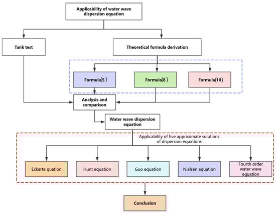
Figure 1.
Research flow frame diagram.
Taking into account the diversity of previous derivations of the dispersion relationship equation for water waves, this paper compares and analyzes several different methods to explore their applicable scope.
- (1)
- When studying the dispersion relationship of surface waves in a liquid, Formula (4) can be transformed into a dispersion relationship formula, Formula (5) [28,29], involving angular frequency, wave number, and water depth.
- (2)
- By considering factors such as the surface tension of the liquid, the shallow depth of the liquid, and the high frequency of surface waves, Formula (4) for water wave dispersion can be transformed into Formula (6) [28,29]. In this case, the dispersion relationship between the angular frequency of water waves, wave number, and water depth can be expressed as Formula (7) [28,29]. By further inserting the formula for the capillary length of water, it can be transformed into Formula (8) [28,29].
- (3)
- Given the nonlinear relation between the frequency of surface waves and their wavelength, Formula (4) can be transformed into Equation (9) [28,29] when In such a case, the dispersion relationship between the angular frequency and wave number of water waves is provided by Equation (10) [28,29]. This equation is applicable to shallow water depths and low frequencies of micro-amplitude waves.
In the Equations (6)–(10), represents the density of free-surface liquid, is the surface tension of the liquid, is the capillary length of water, and is the wave number.
3. Error Analysis of Approximate Solutions of Water Wave Dispersion Equations
3.1. Approximate Method Based on Eckart Formula
In 1952, Eckart [30] proposed an approximate direct solution formula for the dispersion equation of water waves:
Despite the fact that the given formula (i.e., Equation (11)) can quickly calculate the value of based on wave period and water depth, its maximum relative error reaches 5%, which may be considered as not precise enough in some application scenarios [31]. The relative error here is defined as Relative Error = , where represents the approximate solution obtained from each formula and represents the precise solution computed through iteration by the computer.
In order to improve the accuracy of this formula, relevant corrections were made, with the expectation of raising the precision of the formula to 0.05%, thus making it more reliable in actual applications. It is worth mentioning that the improved formula maintains consistent effectiveness throughout the entire relative water depth range. The improved form of the Eckart dispersion relationship is defined as where is the approximate value given by Equation (11), is a suitable correction function, and and are constants. The form of , which tends to zero for both and , is as follows:
Here, and are normal numbers, which are determined by minimizing the numerical solution of the exact dispersion relationship and the improved approximate result.
The least squares method is used to process the 1000 points ranging from with a least squares method, and for convenience of use, the results are rounded to four decimal places to obtain and by substituting the data into the transformation to obtain Equation (13).
In this formula, represents the newly improved dispersion relationship approximation, and is the maximum relative error of −0.044% when the relative water depth approaches zero or infinity, and the formula takes the form of:
We can then determine , and to obtain and substitute them into the following formula to obtain a simplified function:
3.2. McKee Method
McKee [32], based on Eckart’s formula, proposed that the following variant can be obtained:
Here, using in place of , the angular frequency used is , so:
If , then . Hence, in this case, the wave speed, represented by , is:
Then, using the limit properties of hyperbolic functions, we obtain:
For deep water or short wave scenarios, the Eckart approximate formula (Equation (23)) for the limit is:
Eckart’s approximation approximates wave depth to within a factor of about 7, with the maximum error in wavelength being approximately 5%. Formula (23) yields results as good as or better than Formula (11), possibly with an advantage in overestimating wavelength to take into account the nonlinear effects.
It is worth mentioning that all the approximations suggested by Formula (23) can be expressed in the form below:
When = 2, this formula becomes Formula (11). After numerical analysis, Fenton and McKee found that when = 1.49, the maximum relative error between the approximate formula and the exact solution obtained from the dispersion equation is smallest. Therefore, they approximately took = 3/2 and obtained the following simplified form:
By substituting , and , we can obtain:
3.3. Hunt Method
The Hunt [4] method considers the most commonly used iterative equation for calculating k in Formula (3). Using this method, an improved k estimate can be calculated from the equation:
A given set of different values can then be used to construct the data (). A second-degree regression curve is fitted to the constructed data points to obtain .
If , it can be approximated by Padé approximation as:
Later, in 1979, Hunt [5] adopted a more advanced 6th-order Padé approximation to obtain a more accurate dispersion equation approximation formula, which takes the following form:
In the equation, D1 = 0.6667, D2 = 0.3556, D3 = 0.1608, D4= 0.0632, D5 = 0.0217, and D6 = 0.0065.
3.4. Nielsen Method
The general form of the approximation is as follows:
Because of and , , then
The shallow water coefficient is given by the group velocity
Continuing on, we can derive:
For many practical refraction calculations, it is assumed that the terrain has straight and parallel contours, thus making Snell’s law [5] applicable.
If , it means that we start from deep water.
If and are both within , we can obtain.
Considering only the energy loss due to friction, the energy flux equation is:
From , , we have:
From , , we have:
If , then given .
Then, , which can be simplified to:
In any water depth condition, the relative error of Equation (57) is between 0.5% and 0.12%. In 2002, Nielsen [33] further optimized Equation (57) as follows:
3.5. Logarithmic Fitting Approximation Method
Guo used the logarithmic fitting method to approximate the dispersion equation in 2002 [34]. He proposed that for a nonlinear curve, if the expressions of its two asymptotes could be found, it could be combined into a single expression using the logarithmic fitting method. Guo considered two limiting cases (), and used the logarithmic fitting method to combine the expressions, obtaining:
According to Taylor’s formula [35], the fourth-order dispersion relationship can be derived as follows, assuming .
From , we have:
We can further obtain:
Then, . It can be deduced that the momentum equation is:
From , where represents the velocity of the still water, the following equation is derived from the above formula:
Equation (71) can be simplified to:
By eliminating from the above two equations, we get:
If , then the dispersion relation is as follows:
If , then:
By rearranging Equation (77), we ultimately arrive at:
4. Experimental Verification
Verifying the approximate solutions of the dispersion relationship is crucial for providing a scientific foundation for engineering design and minimizing potential risks. The purpose of the experiments is to assess the accuracy and reliability of these solutions under different water depth conditions. This ensures the selection of the most appropriate dispersion relationship for solving the equation, tailored to specific engineering requirements. In the context of natural disaster prediction, the propagation characteristics of water waves are closely linked to phenomena such as floods and storm surges.
4.1. Experiment Equipment
The verification experiment was conducted in a long tank measuring 60 m in length, 1.2 m in width, and 1.0 m in height. The objective was to achieve conditions conducive to long wave propagation, thereby enabling a more accurate study of the wave’s propagation characteristics. At one end of the tank, a water wave generator (model WA-9899) with a frequency range of 1–50 Hz was installed (see Figure 2C). The WA-9899 waveform generator is manufactured by Rigol Technologies, a leading company based in Beijing, China. This device is driven by a mechanical push rod and is capable of producing true plane incident waves, which ensures both stability and repeatability of the waveform. By adjusting the frequency of the WA-9899 water wave generator, various wavelengths could be produced to comprehensively examine the dispersion characteristics of the waves. To ensure measurement accuracy, we employed a high-precision DY300 digital wave height meter. The DY300 Digital is manufactured by Hantek, based in Shenzhen, China, a renowned producer of electronic test equipment, including oscilloscopes and waveform generators, known for offering affordable and reliable solutions for educational, laboratory, and industrial applications. The DY300 digital wave height meter operates by using sensors, such as capacitive, resistive, or ultrasonic transducers, placed at a certain depth below the water surface to detect fluctuations in the water level caused by waves. As waves pass over the sensors, they measure the changes in distance or pressure and transmit the data to the digital processor. The analog signals are then converted into digital form through an analog-to-digital converter (ADC), ensuring high accuracy. This instrument’s multi-channel concentrator can simultaneously collect data from up to 128 channels at a sampling rate of 1 kHz per channel while maintaining very high accuracy. The system calculates various wave parameters, such as significant wave height and peak wave height, based on the recorded fluctuations, and displays the results on a digital screen. Additionally, the DY300 often includes a data logging feature, allowing wave height data to be stored and accessed for further analysis, making it a valuable tool for monitoring wave behavior over time in marine environments.
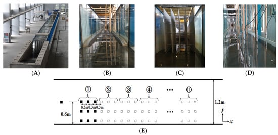
Figure 2.
Experimental water tank and test equipment. (A) The panorama of the test water tank layout shows that the length of the water tank is 60 m, the width is 1.2 m, and the height is 1 m; (B) The elevation of the test tank layout shows that the sides are supported by wooden frames; (C) A water wave generator of model WA-9899 with a frequency range of 1–50 HZ; (D) DY300 digital wave height meter; (E) In the schematic diagram of the test water tank layout, 0.6 m represents three rows of wave altimeters, each row is 0.3 m apart, the total width of the three rows is 0.6 m, and 0.3 m is the transverse interval of the wave altimeter. The squares here represent the wave height meter. Numbers 1–11 represent groups of three columns, and a total of 11 groups were measured.
4.2. Experiment Methods
In this experiment, in order to study the influence of different frequencies and water depths on the characteristics of water waves, we used a WA-9899 model water wave generator to generate stable sine shape waves. The experimental steps are as follows: First, the working parameters of the water wave generator are set, and the frequency is adjusted from 0.5 to 1.5 Hz to cover the influence of low-frequency to medium-frequency waves. For each frequency, three different water depths 0.1 m, 0.15 m, and 0.2 m are selected to examine how these water depths influence wave propagation characteristics and dispersion relations, and the characteristics are observed.
We used the DY300 digital wave height meter to measure the wavelength accurately, which can record the wave height change with high precision and feedback the wave parameters immediately. The distribution of waveforms showed a clear symmetry, with the waves being evenly distributed on both sides of the water tank’s width. This symmetry implies that the wave patterns on one side of the tank mirror those on the other, creating a balanced wave field. As a result, in the experiment, it was sufficient to measure only the waveform corresponding to half the width of the water tank. This approach not only simplifies the data collection process but also ensures that the measurements accurately represent the entire wave behavior, as the other half of the tank will exhibit an identical waveform.
The wave height sensor was set at the front end of the waveguide at a distance of 3 m and then three wave height sensors were set in each row towards the groove wall at a spacing of 0.3 m in the middle of the water tank. Nine wave altimeters formed a group of three rows. After measuring the waveform at the original position of the measure equipment using a wave height sensor, the wave height sensor needed to be moved to the next position. Afterwards, the above method was used to measure all wave heights in the experimental areas ① to ⑪ again. The position distribution of the wave height meter shown in Figure 2E refers to the experimental images measured by the wave height meter.
4.3. Measurement Errors and Experimental Errors
To ensure the reliability of the data, the experiment was repeated at least three times for each water depth and frequency condition. This repetition allowed for a more comprehensive analysis and helped to account for any variations or inconsistencies in the results. Throughout the experimental process, each dataset was collected multiple times to capture the dynamic characteristics of wave propagation and to minimize the impact of random errors. After the data were acquired, it underwent a thorough processing phase. This included filtering out any noise or interference that could distort the results, followed by calculating the average wavelength for each test condition. The corresponding values for different frequencies and water depths were then carefully recorded, ensuring that the data accurately reflected the influence of these variables on the wave behavior. This rigorous approach enhanced the precision and reliability of the findings, providing a solid foundation for further analysis. High-precision measurement instruments, such as wave height meters and pressure sensors, should be used, and measurements should be taken at multiple points and with high-frequency sampling to improve accuracy. Data should be processed through smoothing and averaging to reduce random fluctuations, and appropriate theoretical models should be used for interpretation. Regular calibration of instruments and comparison with known theoretical or experimental results help verify reliability.
To reduce experimental errors in water wave experiments and ensure the accuracy and reliability of results, several key strategies should be employed. The models employed in this study were based on idealized conditions, assuming an incompressible, non-viscous fluid with constant water density and surface tension. First, precise control of experimental conditions is essential, including maintaining uniform water depth, clean water quality, and stable temperature. The wave source should be stable, with accurate control of frequency and amplitude to generate consistent waves. External disturbances, such as air flow or vibrations, should be minimized by isolating the experimental setup. Initial conditions, such as a calm water surface and stable waveforms, must be carefully controlled, and boundary conditions should be optimized to avoid reflection errors.
Additionally, viscosity effects and turbulence interactions should be considered, and multiple repetitions of the experiment can help reduce random errors. To reduce water viscosity during experiments, several methods can be applied. Heating the water to around 30 °C lowers viscosity, but temperature changes should be controlled to avoid affecting other conditions. Using purified or deionized water helps remove impurities that may increase viscosity. Avoid adding substances like salts or sugars that can thicken the water, and minimize air bubbles by adding water slowly or using degassing equipment. Keeping the water clean by filtering it regularly and using low-concentration solutions will also help maintain consistent viscosity. In some cases, low-viscosity liquids can be used as an alternative to water to reduce the impact of fluid resistance in experiments. These liquids, such as alcohols or specially formulated fluids, flow more easily and have a lower resistance to deformation compared to higher-viscosity substances like water with higher impurity levels. The use of low-viscosity liquids can simplify the analysis of fluid dynamics, as they reduce frictional effects and minimize the occurrence of turbulent flow, which may interfere with accurate wave measurements. These liquids are also less likely to exhibit complex behavior, such as excessive drag or energy dissipation, making wave propagation studies more predictable and straightforward. This approach not only enhances the precision of the experiments but also supports the development of more robust models and conclusions in fluid dynamics research.
4.4. Eexperimental Data
By incorporating the experimental data into Figure 3, a comprehensive analysis of water wave propagation characteristics can be conducted. A distinct trend emerges: as the frequency increases from 0.5 to 1.5, an inverse relationship between frequency and wavelength is observed at water depths of 0.1 m, 0.15 m, and 0.2 m. Specifically, when the water depth is set at 0.1 m, the wavelength decreases from 1.95 m to 0.57 m, resulting in an amplitude reduction of approximately 70.77%. At a water depth of 0.15 m, the wavelength decreases from 2.42 m to 0.63 m, representing a reduction of approximately 73.97%. For a water depth of 0.2 m, it reduces from 2.68 m to 0.65 m, reflecting a decline of approximately 75.75%.
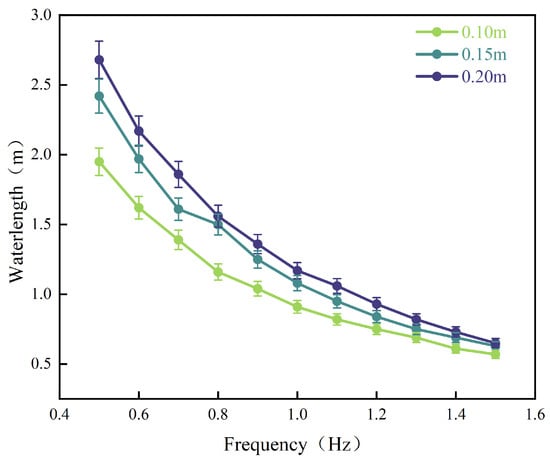
Figure 3.
Variation curves of different frequencies and water depths, corresponding to actual wavelengths.
These findings show that as frequency increases, the wavelength rapidly shortens, highlighting the dispersion properties inherent in water waves. Additionally, it is clear that water depth plays a significant role in determining wavelength behavior. Specifically, wavelengths tend to increase as water depth increases—an observation closely tied to the dynamics of wave propagation in different water depths. In deeper waters, where disruptions are minimal, conditions favor longer wavelengths, while in shallower areas, the restrictions imposed by the shallowness lead to shorter wavelengths.
5. Comparison of Results
5.1. Comparison of Previous Dispersion Formulas and Experimental Data
Through a comparative analysis of previous theories and the relationships among wavelength, frequency, and water depth, we can gain a deeper understanding of the characteristics of water wave propagation. Figure 4 illustrates the relationship between angular frequency and wave number in different water conditions as derived from earlier theories and the dispersion formula for water waves. In these diagrams, the horizontal axis represents angular frequency while the vertical axis denotes wave number. Wave number is defined as the number of waves per unit length and is commonly employed to describe wave propagation characteristics. Conversely, angular frequency is associated with wave frequency and effectively reflects the dynamic behavior of waves.
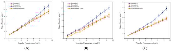
Figure 4.
Relationship between Angular Frequency and Wave Number based on different formulas and experimental value in different water depth respectively. (A).water depth h = 0.1 m. (B) water depth h = 0.15 m. (C) water depth h = 0.2 m.
By analyzing the data in Figure 4, we can conclude that there is an intrinsic correlation between the incident frequency of water waves and their wavelength. These charts visually show how theoretical formulas, namely Formulas (5), (8), and (10), compare to actual measurements at different water depths and different frequencies. Under different water depth conditions, the test values and Equations (5) and (8) show highly consistent trends and similar data sizes, especially under short wavelength conditions, the three almost perfectly coincide. With the increase of wave number 3 to 11, the data gap between the corresponding angular frequency of Formula (10) and Formulas (5) and (8) and the actual measured value gradually increases, showing that the degree of dispersion becomes more obvious with the increase of water depth.
The above conservation demonstrates that using Formulas (5) and (8) to describe the dispersion relationship in a shallow water environment is not only straightforward but also highly accurate when addressing nonlinear water wave problems. These formulas provide a simplified yet reliable approach to understanding wave behavior in shallow waters, where traditional, more complex methods may be computationally intensive or difficult to apply. By utilizing these formulas, one can efficiently model wave propagation, taking into account the unique characteristics of shallow water, such as the influence of the seafloor and water depth. Furthermore, the accuracy of these formulas across different shallow water conditions ensures their practical applicability in real-world scenarios, offering a robust tool for both theoretical analysis and engineering applications. This makes them particularly useful for studies on coastal dynamics, marine infrastructure design, and environmental impact assessments related to water waves.
However, in the experimental data, Formula (10) exhibits noticeable deviations, particularly as the wave number increases. Notably, as the water depth also increases, the deviation becomes more pronounced. This trend indicates that Formula (10) may not fully account for the complexities of wave dynamics under varying conditions, especially at higher wave numbers and deeper water depths. This observation suggests that, under certain conditions—such as low wave numbers where capillary effects are minimal—it may be reasonable to ignore the capillary phenomenon. By neglecting these effects in such scenarios, the model can be simplified, making it more efficient and easier to apply. This simplification could lead to more practical and accurate results in many real-world applications, such as coastal engineering and wave forecasting. However, for more precise predictions in environments with higher wave numbers or when capillary forces play a significant role, further refinement of the model would be necessary. Thus, adjusting the model based on specific conditions, such as water depth and wave number, could enhance its applicability and accuracy in a wider range of practical situations.
5.2. Relative Error Analysis
The MATLAB 2020b (Version 9.9) software program was employed to iteratively solve the aforementioned transcendental equation. The selection and configuration of the transcendental equation represent a critical step in the iterative calculation process. Within the MATLAB environment, a specialized script is developed that leverages its robust numerical computation capabilities to establish initial conditions, iteration accuracy, and convergence criteria. The Newton iteration method or alternative numerical solutions are utilized to ensure high efficiency and precision throughout the iterative procedure. During the iterative calculations, each step’s results are closely monitored to assess convergence. In every iteration, MATLAB computes a new output value based on the current input value and compares it with the previous result to determine whether it falls within the specified error range. This iterative process continues until a predetermined level of accuracy is achieved. Upon completion of the iterations, experimental measurements were conducted to obtain actual data regarding wavelength, frequency, and water depth. By comparing these experimental results with those derived from MATLAB calculations, we can conduct an in-depth analysis of the relative error between direct solution formulas and theoretical derivation formulas. To this end, we calculated the relative error between experimental outcomes and theoretical values, which has been organized into Table 1 below.

Table 1.
Relative error (100%) between iterative values and approximate solutions obtained from the various methods.
Table 1 clearly shows that the calculation errors for Eckart’s Formula (11) and McKee’s modified Formula (28) are minimal across different water depths, with a maximum relative error of approximately 0.3%. These formulas demonstrate high accuracy in predicting wave dispersion under various conditions. While the relative error of Formula (59), derived from logarithmic fitting, is larger, it becomes notably more accurate when the viscosity coefficient of water is higher, especially in deep water. Under these conditions, the error can be reduced to as low as 0.2%. In shallow water, Formulas (57), (58) and (78) show very small relative errors of about 0.1%, confirming their reliability and high precision. These formulas are not only computationally efficient but also exhibit strong performance in practical engineering applications.
The results highlight that Eckart’s and McKee’s formulas provide excellent accuracy across varying water depths, while the logarithmic fitting formula proves particularly effective for deep water conditions where viscosity plays a more significant role. Furthermore, Formulas (57), (58) and (78) offer exceptional accuracy in shallow water, ensuring they are reliable tools for engineers working with wave dispersion in coastal and marine environments.
According to the data presented in Figure 5A, Eckart’s formula exhibits some accuracy deviation, particularly under conditions of high wave numbers. This suggests that Eckart’s formula may not be the optimal choice in such cases, as its results differ significantly from those of the other methods. However, it is important to note that all other methods, except for Eckart’s, show a high degree of accuracy and consistency. These methods maintain stable computational performance in the high wave number range, producing similar results. This consistency not only validates the reliability of these methods but also provides valuable support and reference for research in related fields.
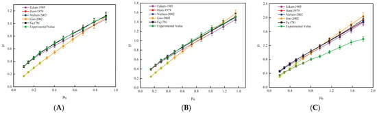
Figure 5.
Comparison of the four direct solution formulas of the dispersion relationships. (A) The relative error analysis between Eckart’s formula and the HUNT, N-S, and GUO formulas. (B) The relative error analysis between Eckart’s formula and the N-S, GUO, and fourth-order formulas. (C) The relative error analysis between the iterative algorithm and the N-S, fourth-order, and HUNT formulas.
Figure 5B compares the wave dispersion equation from the fourth-order explicit solution of Equation (78) with three different formulas: GUO, N-S, and HUNT. The comparison reveals that the results of Equation (78) align closely with the solutions obtained from the other formulas. This strong agreement further demonstrates the accuracy of Equation (78) and its effectiveness as a fourth-order explicit solution to the wave dispersion equation. This consistency ensures that Equation (78) provides a reliable and practical solution for wave dispersion analysis in real-world applications.
Figure 5C presents a comparison between the exact solution obtained through a computer iterative algorithm and the results from the other three direct solution formulas. From this comparison, we can draw several key conclusions: when the wave number is small (i.e., the wavelength is long and the water depth is relatively shallow compared to the wavelength), Formula (56) derived in this study, along with the N-S formula from the Taylor series expansion, shows a high degree of agreement with the iterative results. This confirms their applicability under these specific conditions. As the wavelength decreases and the water depth-to-wavelength ratio increases, it is observed that while the aforementioned formulas begin to show limitations in directly solving the dispersion relationship, they still maintain a wide range of applicability and reliability in the long wave range considered in this study. This finding underscores the importance of clearly defining the applicable range of each formula under different working conditions and offers a valuable reference when compared to the iterative solution.
To further validate the practical utility of these direct solution formulas, a wave generation experiment was conducted in the experimental tank. In this phase, experimental data collected under various water depth conditions were integrated into the calculation model, which included the five direct solution formulas discussed earlier. This approach facilitated a comparative analysis between the measured data and theoretical predictions, allowing for a rigorous assessment of the accuracy of these formulas.
The detailed comparative analysis in Figure 6 presents a thorough comparison between the experimental measurement data under various water depth conditions and the analytical solutions obtained from the distributed direct solution formulas. Notably, the formula proposed by Guo shows a significant deviation from the actual measured curves after applying the logarithmic fitting method. This clearly indicates that the applicability of this formula is limited under long wave conditions, as there is a substantial error between the predicted results and the measured values. This considerable discrepancy undermines the reliability of the formula for practical applications.
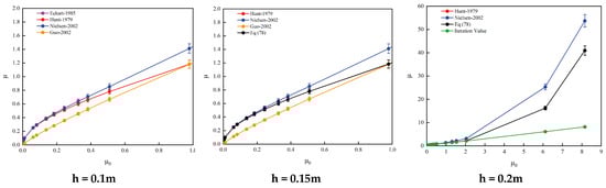
Figure 6.
Comparison of experimental data with five direct solution formulas of water depth h = 0.1 m, h = 0.15 m, and h = 0.2 m, respectively.
Similarly, the residual curves from other analytical methods under long wave conditions also fail to match the measured data closely, with notable errors remaining. Additionally, as the wave number increases, the deviation between the predicted results and the measured data from Eckart’s formula becomes more pronounced, especially under shallow water conditions. This suggests that the Eckart formula requires optimization and adjustment within the context of the current research to enhance its prediction accuracy in shallow water scenarios.
In contrast, several other formulas derived in this study, including the Hunt formula, the N-S formula, and the fourth-order equation, exhibit high prediction accuracy. These formulas demonstrate a good agreement with the measured data, confirming their validity and accuracy in solving the nonlinear dispersion relation of water waves.
6. Discussion and Conclusions
This paper mainly discusses the water wave dispersion relation, aiming to calculate the water wave height and wavelength accurately by comparing the improved dispersion relation formula with the conventional three dispersion relation formulas. According to the study, three conclusions can be drawn:
- (1)
- Under long wave conditions, Equations (5) and (8) provide a more accurate representation of the relationship between wavelength and frequency, while also accounting for the actual effects of capillarity and surface tension. This aligns well with empirical observations. However, Equation (10) exhibits a significant deviation from experimental data when the wave number is small, suggesting that water waves no longer adhere to the linear dispersion relationship under these circumstances. Consequently, in engineering applications, the nonlinear dispersion Equation (5) can be employed to effectively describe the dispersion characteristics of water waves.
- (2)
- Eckart’s Formula (11) and Fenton and McKee’s modified Formula (28) perform well in terms of calculation error, with a maximum relative error of only about 0.3%, which is applicable to any water depth range. Formula (59) gradually becomes accurate under deep water conditions, with a minimum relative error of 0.2%. The relative errors of Equations (57), (58), and (78) in shallow water waves are all maintained at about 0.1%, and these formulas are suitable for the calculation of water wave height in the water wave dispersion relationship under engineering conditions, with high efficiency and high precision.
- (3)
- As the wave number increases, the deviation of the Eckart formula becomes pronounced under shallow water conditions, indicating that further optimization of this formula is necessary to enhance the accuracy of analytical solutions. In contrast, the HUNT formula, the N-S formula, and the fourth-order Equation (78) derived in this study demonstrate high accuracy and can be regarded as optimal formulas for addressing the nonlinear dispersion relationship of water waves. In practical applications, considering nonlinear factors, Equation (78) will be employed to establish the correspondence between frequency and wavelength. Furthermore, while the explicit solution obtained through Taylor expansion exhibits high accuracy in shallow water conditions, its accuracy diminishes in intermediate depths and fails to hold in deep water scenarios.
This study provides valuable insights into the dispersion relationship of water waves, particularly in shallow and medium water depths. However, there are several limitations that should be addressed in future research. The findings may not be directly applicable to deep water or high-turbulence conditions, as these environments often involve additional factors such as wind waves, ocean currents, or variations in salinity that can influence wave behavior. Furthermore, the models used in this study were based on idealized assumptions, such as constant water density and surface tension, which may not accurately represent the complexity and variability of real-world marine environments. The experimental data used for model validation were also limited to a specific range of wave frequencies, excluding extreme or rare wave events that could exhibit different wave dynamics. Additionally, to improve computational efficiency, simplified numerical methods were employed, which may have overlooked more complex nonlinear interactions between waves. Future research should aim to expand the range of experimental conditions to include deeper water and high-turbulence scenarios, account for environmental variability, and incorporate more advanced computational techniques to better capture the full complexity of wave dispersion. This would improve the accuracy of the models and extend their applicability to a wider range of real-world situations. Exploring the influence of varying fluid properties and nonlinear wave interactions would also be crucial for developing more reliable and comprehensive models.
Building on the findings of this study, there are several promising avenues for future research and practical engineering applications. In terms of engineering applications, the improved dispersion relation formulas can significantly enhance the design and optimization of marine infrastructure, particularly in the construction of port breakwaters, jetties, and dock structures. By accurately predicting wave behavior, these formulas can help engineers design structures that are better able to withstand dynamic wave forces, ensuring the long-term stability and resilience of coastal and offshore facilities. Furthermore, the study’s insights into the nonlinear wave behavior and the limitations of existing formulas, particularly in shallow and medium water depths, can inform more precise and efficient designs for coastal protection and harbor development projects. The formulas derived from this research can also be integrated into hydrodynamic models to improve predictions of wave height and wavelength in various marine environments, ultimately contributing to safer, more sustainable infrastructure.
For future research, the exploration of real-world conditions, such as varying water properties (e.g., salinity, temperature) and complex environmental factors (e.g., wind waves, ocean currents), would further strengthen the models’ applicability to a broader range of scenarios. Additionally, integrating more advanced computational methods [36], such as computational fluid dynamics (CFD) [37,38] or machine learning techniques, could enhance the modeling of nonlinear interactions between waves, currents, and seabed conditions.
In summary, this research not only offers valuable tools for more accurate wave predictions but also lays the foundation for further innovations in coastal engineering and oceanographic research. It highlights the importance of refining existing models to account for environmental complexities and provides a clear pathway for future studies to improve both the theoretical and practical aspects of wave dispersion analysis.
Author Contributions
Conceptualization, S.Z. and G.L.; methodology, S.Z.; software, S.Z. and G.L; validation, G.L.; formal analysis, S.Z.; investigation, G.L.; resources, G.L.; data curation, G.L.; writing—original draft preparation, S.Z.; writing—review and editing, G.L. and S.Z.; visualization, S.Z.; supervision, G.L.; project administration, S.Z. and G.L.; funding acquisition, G.L. All authors have read and agreed to the published version of the manuscript.
Funding
We would like to express our sincere gratitude to the National Natural Science Foundation for their support of the project titled “Damage Monitoring Research of Offshore Wind Power Single-Pile Support Structure Based on High Order Statistics” (Project Number: 51779224), as well as the project “Study on Bearing Capacity Characteristics of Large Diameter Grouting Casing for Offshore Wind Power Under Complex Load” (Project No. 51579221). Additionally, We extend our appreciation to the Zhejiang Provincial Department of Science and Technology for their funding under the Zhejiang Province Spearhead Research and Development Plan (Project Number: 2024C03031), which has facilitated our experiments at Zhejiang University. Furthermore, We are I am deeply grateful to the professors and experts from the School of Civil Engineering and Architecture at Zhejiang University for their invaluable guidance, as well as to the institution itself for providing us with this methodology.
Data Availability Statement
Data are contained within the article.
Conflicts of Interest
The authors declare no conflicts of interest.
References
- Kharfia, B.; El-Amine, C.; Eslamian, S. Modeling the Propagation of the Submersion Wave in Case of a Dam Break: Case of the Gargar Dam, Algeria. In Flood Handbook; CRC Press: Boca Raton, FL, USA, 2022; pp. 509–518. [Google Scholar]
- Kharfia, B.; Amine, C.E. Flood risk assessment and management in urban areas: A case study in Bechar City, South Western Algeria. Int. J. Hydrol. Sci. Technol. 2020, 10, 346–363. [Google Scholar] [CrossRef]
- Rattanapitikon, W.Y.; Suwimol, K. Verification and modification of empirical formulas for computing wave shoaling. Ocean Eng. 2018, 152, 145–153. [Google Scholar] [CrossRef]
- Hunt, J.N. Direct solution of wave dispersion equation. J. Waterw. Port Coast. Ocean Eng. 1979, 105, 457–459. [Google Scholar] [CrossRef]
- Nielsen, P. Explicit formulae for practical wave calculations. Coast. Eng. 1982, 6, 389–398. [Google Scholar] [CrossRef]
- Nielsen, P. Explicit solutions to practical wave problems. Coast. Eng. 1984, 1, 66. [Google Scholar] [CrossRef]
- You, Z.J. A close approximation of wave dispersion relation for direct calculation of wavelength in any coastal water depth. Appl. Ocean Res. 2008, 30, 113–119. [Google Scholar] [CrossRef]
- Guo, J. Simple and explicit solution of wave dispersion equation. Coast. Eng. 2002, 45, 71–74. [Google Scholar] [CrossRef]
- You, Z.J. A simple model of sediment initiation under waves. Coast. Eng. 2000, 41, 399–412. [Google Scholar] [CrossRef]
- You, Z.J.; Hanslow, D. Statistical distribution of nearbed wave orbital velocity under irregular waves. In Coasts & Ports 2001: Proceedings of the 15th Australasian Coastal and Ocean Engineering Conference, the 8th Australasian Port and Harbour Conference, Gold Coast, QLD, Australia, 25–28 September 2001; Institution of Engineers: Barton, Australia, 2001. [Google Scholar]
- Eckart, C. The propagation of gravity waves from deep to shallow water. J. Bacteriol. 1952, 172, 3849–3858. [Google Scholar]
- Berkhoff, J.C.W. Mathematical Models for Simple Harmonic Linear Water Waves: Wave Diffraction and Refraction. Ph.D. Thesis, Delft University of Technology, Delft, The Netherlands, 1976. [Google Scholar]
- Berkhoff, J.C.W. Computation of combined refraction-diffraction. Coast. Eng. 1972, 1973, 471–490. [Google Scholar] [CrossRef]
- Chamberlain, P.G.; Porter, D. The modified mild-slope equation. J. Fluid Mech. 1995, 291, 393–407. [Google Scholar] [CrossRef]
- Booij, N. A note on the accuracy of the mild-slope equation. Coast. Eng. 1983, 7, 191–203. [Google Scholar] [CrossRef]
- Porter, D.; Staziker, D.J. Extensions of the mild-slope equation. J. Fluid Mech. 1995, 300, 367–382. [Google Scholar] [CrossRef]
- Agnon, Y. Linear and nonlinear refraction and Bragg scattering of water waves. Phys. Rev. E 1999, 59, R1319–R1322. [Google Scholar] [CrossRef]
- Dl, F.; Batelaan, H. Bragg scattering of free electrons using the Kapitza-Dirac effect—Art. no. 283602. Phys. Rev. Lett. 2002, 28, 89. [Google Scholar]
- Zhou, H. A Higher-Order Depth-Integrated Model for Water Waves and Currents Generated by Underwater Landslides. Ph.D. Thesis, University of Hawaii at Manoa, Honolulu, HI, USA, 2008. [Google Scholar]
- Wang, P.; Lu, D.Q. Homotopy-based analytical approximation to nonlinear short-crested waves in a fluid of finite depth. J. Hydrodyn. 2015, 3, 11. [Google Scholar] [CrossRef]
- Beji, S.; Battjes, J.A. Experimental investigation of wave propagation over a bar. Coast. Eng. 1993, 19, 151–162. [Google Scholar] [CrossRef]
- Beji, S. Improved explicit approximation of linear dispersion relationship for gravity waves. Coast. Eng. 2013, 73, 11–12. [Google Scholar] [CrossRef]
- Kendall, J.; Monroe, K.P. The viscosity of liquids. II. The viscosity-composition curve for ideal liquid mixtures. J. Am. Chem. Soc. 1917, 39, 1787–1802. [Google Scholar] [CrossRef]
- Hutter, K.; Wang, Y. Hydrodynamics of Ideal Liquids. In Fluid and Thermodynamics: Volume 1: Basic Fluid Mechanics; Springer: Cham, Switzerland, 2016; pp. 57–158. [Google Scholar]
- Landau, L.; Lifshitz, E. Chapter I—Ideal Fluids. In Fluid Mechanics; Pergamon: Oxford, UK, 1987; pp. 30–31. [Google Scholar]
- Mei, C.C.; Black, J.L. Scattering of surface waves by rectangular obstacles in waters of finite depth. J. Fluid Mech. 1969, 38, 499–511. [Google Scholar] [CrossRef]
- Porter, D. The mild-slope equations. J. Fluid Mech. 2003, 494, 51–63. [Google Scholar] [CrossRef]
- Mei, C.C.; Nlata, M. Harmonic generation in shallow water waves. In Waves on Beaches and Resulting Sediment Transport; Academic Press: New York, NY, USA, 1972; pp. 181–202. [Google Scholar]
- Mei, C.C.; Liu, P.L. Surface waves and coastal dynamics. Annu. Rev. Fluid Mech. 1993, 25, 215–240. [Google Scholar] [CrossRef]
- Eckart, C. The scattering of sound from the sea surface. J. Acoust. Soc. Am. 1953, 25, 566–570. [Google Scholar]
- Zhang, Y.; Liu, Y. Direct solution of water wave dispersion equation. J. Waterw. Harb. 2015, 36, 8–11+20. [Google Scholar]
- Fenton, J.D.; McKee, W.D. On calculating the lengths of water waves. Coast. Eng. 1990, 14, 499–513. [Google Scholar] [CrossRef]
- Nielsen, P. Teaching Notes on Coastal and Estuarine Processes. Ph.D. thesis, The University of Queensland, Department of Civil Engineering, Brisbane, QLD, Australia, 2002. [Google Scholar]
- Guo, J. Reply to discussion of “Simple and explicit solution to the wave dispersion equation”. Coast. Eng. 2003, 48, 137. [Google Scholar] [CrossRef]
- Zou, Z.L. A new form of higher order Boussinesq equations. Ocean Eng. 2000, 27, 557–575. [Google Scholar] [CrossRef]
- Gao, R.; Wang, W.; Zhou, K.; Zhao, Y.; Yang, C.; Ren, Q. Optimization of a multiphase mixed flow field in backfill slurry preparation based on multiphase flow interaction. ACS Omega 2023, 8, 34698–34709. [Google Scholar] [CrossRef]
- Li, Y.; Nielsen, P.V. CFD and ventilation research. Indoor Air 2011, 21, 442–453. [Google Scholar] [CrossRef]
- Samstag, R.W.; Ducoste, J.J.; Griborio, A.; Nopens, I.; Batstone, D.J.; Wicks, J.D.; Saunders, S.; Wicklein, E.A.; Kenny, G.; Laurent, J. CFD for wastewater treatment: An overview. Water Sci. Technol. 2016, 74, 549–563. [Google Scholar] [CrossRef]
Disclaimer/Publisher’s Note: The statements, opinions and data contained in all publications are solely those of the individual author(s) and contributor(s) and not of MDPI and/or the editor(s). MDPI and/or the editor(s) disclaim responsibility for any injury to people or property resulting from any ideas, methods, instructions or products referred to in the content. |
© 2025 by the authors. Licensee MDPI, Basel, Switzerland. This article is an open access article distributed under the terms and conditions of the Creative Commons Attribution (CC BY) license (https://creativecommons.org/licenses/by/4.0/).