Geometric Properties of the m-Leaf Function and Connected Subclasses ^†

Abstract

In this study, we introduce and explore the properties of the m-leaf function ${\mathcal{Q}}_m$ defined in the open unit disk $\mathbb{D}$, where $m\in \mathbb{N}$, and this function is defined by the relation ${\mathcal{Q}}_m\left(z\right):=1+{\displaystyle \frac{m+1}{m+2}}z+{\displaystyle \frac{1}{m+2}}{z}^{m+1}$. We determine the main geometrical characterization of this function, focusing on its univalency and its sharp bounds for the real and imaginary modulus. Also, we find radius of convexity, and we give a subordination and inclusion result. Using this function, we introduce a new subclass of analytic functions normalized as usual in $\mathbb{D}$ denoted by ${\mathcal{A}}_m^{r,s}$, and an investigation of this class reveals some interesting properties.

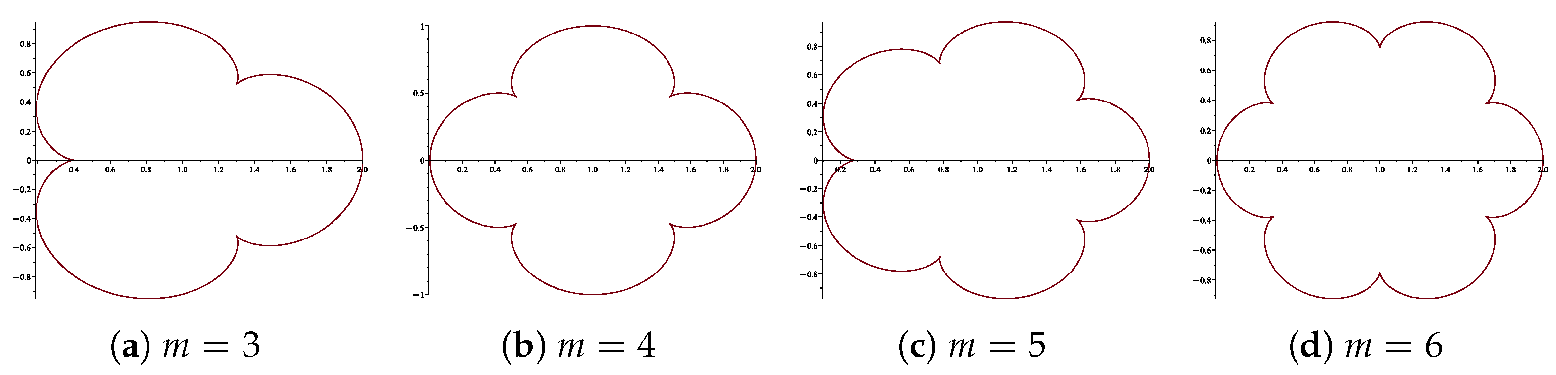
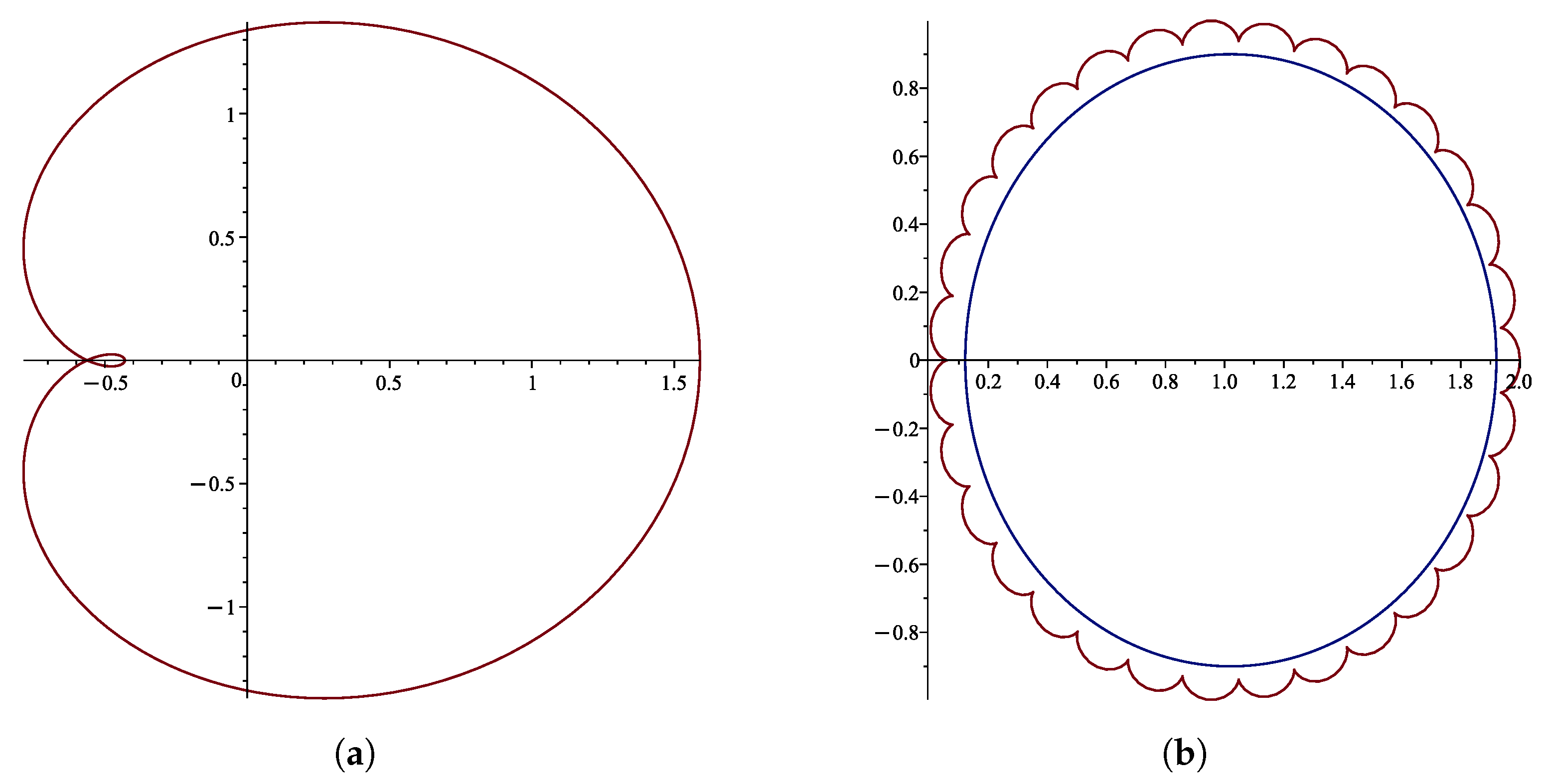
1. Introduction and Preliminary Results for the m-Leaf Function

For $m\in \mathbb{N}:=\{1,2,\dots \}$, we define the m-leaf function by

$${\mathcal{Q}}_m\left(z\right):=1+{\displaystyle \frac{m+1}{m+2}}z+{\displaystyle \frac{1}{m+2}}{z}^{m+1},z\in \mathbb{D},$$

(1)

where $\mathbb{D}:=\{z\in \mathbb{C}:\left|z\right|<1\}$ is the open unit disk in the complex plane. Since ${\mathcal{Q}}_m$ is a polynomial function of degree “$m+1$”, it is obvious that it is analytic in $\mathbb{D}\subset \mathbb{C}$.

We will extend the above function ${\mathcal{Q}}_m$ for $m=0$ by

$${\mathcal{Q}}_0\left(z\right)=1+z,z\in \mathbb{D},$$

and let

$$\mathcal{Q}\left(z\right):=\underset{m\to \infty }{lim}{\mathcal{Q}}_m\left(z\right)=\underset{m\to \infty }{lim}1+{\displaystyle \frac{m+1}{m+2}}z+{\displaystyle \frac{1}{m+2}}{z}^{m+1}=1+z=Q_0\left(z\right),z\in \mathbb{D},$$

(2)

and this function is analytic in $\mathbb{C}$ as a polynomial function.

Remark 1. 

In [1], the author defined and studied a subclass of bounded turning functions connected to a three-leaf function ${\mathcal{Q}}_3\left(z\right):=1+{\displaystyle \frac{4}{5}}z+{\displaystyle \frac{1}{5}}{z}^4$, $z\in \mathbb{D}$. Also, in [2,3], the authors introduced and investigated the properties of different subclasses of analytic functions defined by using the subordination to the four-leaf function given by ${\mathcal{Q}}_4\left(z\right):=1+{\displaystyle \frac{5}{6}}z+{\displaystyle \frac{1}{6}}{z}^5$, $z\in \mathbb{D}$.

In the field of Geometric Function Theory, the geometric image of $\mathbb{D}$ by the different functions is relevant; therefore, many previous papers have dealt with cardioids, limaçons, nephroids, Bernoulli’s lemniscate, etc. Functions that map $\mathbb{D}$ include these types of domains. Since the three-leaf and four-leaf functions were already defined and studied in the above mentioned papers, our first goal is to generalize these previous “leaf-type” functions to the m-leaf function, $m\in \mathbb{N}$, and to underline their main properties.

More generally, the name of the m-leaf function for ${\mathcal{Q}}_m$ stems from the next reasons. Setting $z={\mathrm{e}}^{i\theta }$ with $0\le \theta <2\pi$, that is, $\left|z\right|=1$, we obtain

$${\mathcal{Q}}_m\left({\mathrm{e}}^{i\theta }\right)=1+{\displaystyle \frac{m+1}{m+2}}cos\theta +{\displaystyle \frac{cos\left(m+1\right)\theta }{m+2}}+i\left({\displaystyle \frac{m+1}{m+2}}sin\theta +{\displaystyle \frac{sin\left(m+1\right)\theta }{m+2}}\right),$$

hence

$$Re{\mathcal{Q}}_m\left({\mathrm{e}}^{i\theta }\right)=1+{\displaystyle \frac{m+1}{m+2}}cos\theta +{\displaystyle \frac{cos\left(m+1\right)\theta }{m+2}}=:u\left(\theta \right),$$

(3)

and

$$Im{\mathcal{Q}}_m\left({\mathrm{e}}^{i\theta }\right)={\displaystyle \frac{m+1}{m+2}}sin\theta +{\displaystyle \frac{sin\left(m+1\right)\theta }{m+2}}=:v\left(\theta \right).$$

(4)

For $m\in \mathbb{N}$, let $u:=u\left(\theta \right)$ and $v:=v\left(\theta \right)$. Then, ${\mathcal{Q}}_m\left({\mathrm{e}}^{i\theta }\right)$ is a closed Jordan curve ${\Gamma }_m$ whose parametric equations are

$$\left({\Gamma }_m\right):\left\{\begin{array}{c}u=1+{\displaystyle \frac{m+1}{m+2}}cos\theta +{\displaystyle \frac{cos\left(m+1\right)\theta }{m+2}},\hfill \\ v={\displaystyle \frac{m+1}{m+2}}sin\theta +{\displaystyle \frac{sin\left(m+1\right)\theta }{m+2}},0\le \theta <2\pi ,\hfill \end{array}\right.$$

(5)

and the domain ${\mathcal{Q}}_m\left(\mathbb{D}\right)$ lies inside of ${\Gamma }_m$, with the boundary $\partial {\mathcal{Q}}_m\left(\mathbb{D}\right)={\Gamma }_m$.

We will prove that the curve ${\Gamma }_m$ has “m” cusps at the corresponding points for ${\theta }_k={\displaystyle \frac{\left(2k-1\right)\pi }{m}}$, $k\in \{1,\dots ,m\}$. Thus, from the above parametric equations, we obtain the equation system

$$\left\{\begin{array}{c}{\displaystyle \frac{du}{d\theta }}=-{\displaystyle \frac{m+1}{m+2}}\left(sin\theta +sin\left(m+1\right)\theta \right)=0,\hfill \\ {\displaystyle \frac{dv}{d\theta }}={\displaystyle \frac{m+1}{m+2}}\left(cos\theta +cos\left(m+1\right)\theta \right)=0\hfill \end{array}\right.\iff \left\{\begin{array}{c}sin{\displaystyle \frac{\left(m+2\right)\theta }{2}}cos{\displaystyle \frac{m\theta }{2}}=0,\hfill \\ cos{\displaystyle \frac{\left(m+2\right)\theta }{2}}cos{\displaystyle \frac{m\theta }{2}}=0\hfill \end{array}\right.$$

that is equivalent to

$$\left\{\begin{array}{c}sin{\displaystyle \frac{\left(m+2\right)\theta }{2}}=0\mathit{or}cos{\displaystyle \frac{m\theta }{2}}=0,\hfill \\ cos{\displaystyle \frac{\left(m+2\right)\theta }{2}}=0\mathit{or}cos{\displaystyle \frac{m\theta }{2}}=0,\hfill \end{array}\right.$$

and we conclude that this last equation system has the solutions ${\theta }_k={\displaystyle \frac{\left(2k-1\right)\pi }{m}}$, $k\in \{1,\dots ,m\}$, hence the points $u\left({\theta }_k\right)+iv\left({\theta }_k\right)$, $k\in \{1,\dots ,m\}$ represent the “m” cusps of the curve ${\Gamma }_m$.

In Figure 1a–d, we present the images of ${\Gamma }_m$ for $m\in \{3,\dots ,6\}$, and for the previously mentioned reasons, these show that the domains ${\mathcal{Q}}_m$ look like a leaf with m petals. Note that all of the figures in this article were made by using MAPLE™ (2024 free trial edition) computer software.

Figure 1. The images of ${\Gamma }_m$, $m\in \{3,4,5,6\}$.

If F is an analytic function in $\mathbb{D}$, we say that F is a starlike function with respect to the point $w_0=F\left(0\right)$ if F is univalent in $\mathbb{D}$, and $F\left(\mathbb{D}\right)$ is a starlike domain with respect to $w_0$, that is, the segment $\left[w_0,F\left(z\right)\right]$ is enclosed in $F\left(\mathbb{D}\right)$ for all $z\in \mathbb{D}$:

$$\left\{\lambda F\left(0\right)+(1-\lambda )F\left(z\right):\lambda \in [0,1],z\in \mathbb{D}\right\}\subset F\left(\mathbb{D}\right).$$

It is well known that the function F is starlike with respect to the point $w_0=F\left(0\right)$ if and only if $F^{\prime }\left(0\right)\ne 0$ and

$$Re{\displaystyle \frac{z{F}^{\prime }\left(z\right)}{F\left(z\right)-w_0}}>0,z\in \mathbb{D}.$$

(see, for example, [4], [5] (pp. 167, 202), [6] (p. 42)).

Remark 2. 

1. For all $m\in \mathbb{N}$, the function ${\mathcal{Q}}_m$ is univalent in $\mathbb{D}$.

2. The m-leaf function ${\mathcal{Q}}_m$ is starlike (univalent) in $\mathbb{D}$ with respect to $w_0=1$, and the domain ${\mathcal{Q}}_m\left(\mathbb{D}\right)$ is symmetric with respect to the real axis.

Proof. 

1. For $m\in \mathbb{N}$, let $z_1,z_2\in \mathbb{D}$, such that

$${\mathcal{Q}}_m\left(z_1\right)={\mathcal{Q}}_m\left(z_2\right),$$

which is equivalent to $\left(m+1\right)\left(z_1-z_2\right)=z_2^{m+1}-z_1^{m+1}$. Assuming that $z_1\ne z_2$, then the previous equality is equivalent to

$$m+1=-\left(z_1^m+z_1^{m-1}{z}_2+\cdots +z_2^m\right)$$

which implies

$$m+1=\left|z_1^m+z_1^{m-1}{z}_2+\cdots +z_2^m\right|.$$

(6)

Using the triangle inequality, we easily obtain

$$\left|z_1^m+z_1^{m-1}{z}_2+\cdots +z_2^m\right|\le {\left|z_1\right|}^m+{\left|z_1\right|}^{m-1}\left|z_2\right|+\cdots +{\left|z_2\right|}^m<m+1,z\in \mathbb{D},$$

hence the equality (6) does not hold for any $z_1,z_2\in \mathbb{D}$ with $z_1\ne z_2$. Thus, our initial assumption implies that $z_1=z_2$, and consequently, ${\mathcal{Q}}_m$ is univalent in $\mathbb{D}$.

2. Since ${\mathcal{Q}}_m\left(0\right)=1$, ${\mathcal{Q}}_m^{\prime }\left(0\right)={\displaystyle \frac{m+1}{m+2}}\ne 0$, and

$$\begin{array}{c}Re{\displaystyle \frac{z{\mathcal{Q}}_m^{\prime }\left(z\right)}{{\mathcal{Q}}_m\left(z\right)-{\mathcal{Q}}_m\left(0\right)}}=\left(m+1\right)Re{\displaystyle \frac{1+z^m}{m+1+z^m}}=\left(m+1\right)\left(1-mRe{\displaystyle \frac{1}{m+1+z^m}}\right)\\ \ge \left(m+1\right)\left(1-m\left|{\displaystyle \frac{1}{m+1+z^m}}\right|\right)\ge \left(m+1\right)\left(1-{\displaystyle \frac{m}{m+1-{\left|z\right|}^m}}\right)>0,z\in \mathbb{D},\end{array}$$

it follows that the m-leaf function ${\mathcal{Q}}_m$ is starlike (univalent) in $\mathbb{D}$ with respect to $w_0=1$.

From the fact that $\overline{{\mathcal{Q}}_m}\left(z\right)={\mathcal{Q}}_m\left(\overline{z}\right)$, $z\in \mathbb{D}$, it follows that the domain ${\mathcal{Q}}_m\left(\mathbb{D}\right)$ is symmetric with respect to the real axis. □

2. Main Results

Some remarkable geometric properties of the m-leaf function will be presented in the next four theorems. These results deal with covering, distortion, and bound inequalities, and are followed by one connected with the radius of convexity for this function.

Theorem 1. 

$\left(i\right)$ The next covering inequalities for ${\mathcal{Q}}_m$ hold for all $m\in \mathbb{N}$:

$$1-{\displaystyle \frac{m+1}{m+2}}\rho -{\displaystyle \frac{1}{m+2}}{\rho }^{m+1}\le |{\mathcal{Q}}_m\left(z\right)|\le 1+{\displaystyle \frac{m+1}{m+2}}\rho +{\displaystyle \frac{1}{m+2}}{\rho }^{m+1},\left|z\right|\le \rho <1.$$

(7)

$\left(ii\right)$ If $m\in \mathbb{N}$, we have the next distortion result:

$${\displaystyle \frac{m+1}{m+2}}\left(1-{\rho }^m\right)\le |{\mathcal{Q}}_m^{\prime }\left(z\right)|\le {\displaystyle \frac{m+1}{m+2}}\left(1+{\rho }^m\right),\left|z\right|\le \rho <1.$$

(8)

$\left(iii\right)$ For $m\in \mathbb{N}$, the inequality $Re{\mathcal{Q}}_m\left(z\right)>0$ holds for all $z\in \mathbb{D}$.

Proof. 

$\left(iii\right)$ Using some well-known elementary inequalities, the last result follows easily, as is shown below:

$$\begin{array}{cc}\hfill Re{\mathcal{Q}}_m\left(z\right)& =Re\left(1+{\displaystyle \frac{m+1}{m+2}}z+{\displaystyle \frac{1}{m+2}}{z}^{m+1}\right)=1+Re\left({\displaystyle \frac{m+1}{m+2}}z+{\displaystyle \frac{1}{m+2}}{z}^{m+1}\right)\hfill \\ \hfill & \ge 1-\left|{\displaystyle \frac{m+1}{m+2}}z+{\displaystyle \frac{1}{m+2}}{z}^{m+1}\right|\ge 1-{\displaystyle \frac{m+1}{m+2}}\left|z\right|-{\displaystyle \frac{1}{m+2}}{\left|z\right|}^{m+1}\hfill \\ \hfill & >1-{\displaystyle \frac{m+1}{m+2}}-{\displaystyle \frac{1}{m+2}}=0,z\in \mathbb{D}.\hfill \end{array}$$

(i) We easily see that for $\left|z\right|\le \rho <1$, we have

$$\begin{array}{cc}\hfill |{\mathcal{Q}}_m\left(z\right)|=\left|1+{\displaystyle \frac{m+1}{m+2}}z+{\displaystyle \frac{1}{m+2}}{z}^{m+1}\right|& \le 1+{\displaystyle \frac{m+1}{m+2}}\left|z\right|+{\displaystyle \frac{1}{m+2}}{\left|z\right|}^{m+1}\hfill \\ \hfill & \le 1+{\displaystyle \frac{m+1}{m+2}}\rho +{\displaystyle \frac{1}{m+2}}{\rho }^{m+1},\hfill \end{array}$$

and

$$\begin{array}{cc}\hfill |{\mathcal{Q}}_m\left(z\right)|=\left|1+{\displaystyle \frac{m+1}{m+2}}z+{\displaystyle \frac{1}{m+2}}{z}^{m+1}\right|& \ge 1-{\displaystyle \frac{m+1}{m+2}}\left|z\right|-{\displaystyle \frac{1}{m+2}}{\left|z\right|}^{m+1}\hfill \\ \hfill & \ge 1-{\displaystyle \frac{m+1}{m+2}}\rho -{\displaystyle \frac{1}{m+2}}{\rho }^{m+1},\hfill \end{array}$$

which prove the double inequality (7).

(ii) From (1), we have

$${\mathcal{Q}}_m^{\prime }\left(z\right)={\displaystyle \frac{m+1}{m+2}}\left(1+z^m\right),z\in \mathbb{D},$$

and using a similar proof like those of the item $\left(i\right)$, we easily obtain the distortion result given by (8). □

Remark 3. 

Taking $\rho \to 1^{-}$ in the right-hand sides of the inequalities (7) and (8), we see that for all $m\in \mathbb{N}$, the following inequalities hold:

$$|{\mathcal{Q}}_m\left(z\right)|<2,z\in \mathbb{D},\left|{\mathcal{Q}}_m^{\prime }\left(z\right)\right|<{\displaystyle \frac{2(m+1)}{m+2}},z\in \mathbb{D}.$$

Therefore, ${\mathcal{Q}}_m$ is a bounded function while the second inequality represents a distortion property in $\mathbb{D}$.

Theorem 2. 

The following sharp (i.e., best possible) inequalities hold for $m\in \mathbb{N}$:

$$\begin{array}{cccc}0\le Re{\mathcal{Q}}_m\left({\mathrm{e}}^{i\theta }\right)\le 2,\hfill & \mathit{if}\hfill & m\hfill & \mathit{is}\mathit{even},\hfill \\ 1-cos{\displaystyle \frac{\pi }{m+2}}\le Re{\mathcal{Q}}_m\left({\mathrm{e}}^{i\theta }\right)\le 2,\hfill & \mathit{if}\hfill & m\hfill & \mathit{is}\mathit{odd},\hfill \end{array}$$

and

$$\left|Im{\mathcal{Q}}_m\left({\mathrm{e}}^{i\theta }\right)\right|\le \left\{\begin{array}{ccc}1,\hfill & \mathit{if}\hfill & m=4p,\hfill \\ cos{\displaystyle \frac{\pi }{2(m+2)}},\hfill & \mathit{if}\hfill & m=4p-1,\hfill \\ cos{\displaystyle \frac{\pi }{m+2}},\hfill & \mathit{if}\hfill & m=4p-2,\hfill \\ cos{\displaystyle \frac{\pi }{2(m+2)}},\hfill & \mathit{if}\hfill & m=4p-3,\hfill \end{array}\right.$$

where $p\in \mathbb{N}$.

Proof. 

Using the notation of (5), from (3) and the previous computations, we see that $u=u$ attains the extremal values at the solutions of the equation

$$sin{\displaystyle \frac{\left(m+2\right)\theta }{2}}cos{\displaystyle \frac{m\theta }{2}}=0$$

that are

$${\theta }_k={\displaystyle \frac{2k\pi }{m+2}}\mathrm{and}{\widehat{\theta }}_l={\displaystyle \frac{(2l+1)\pi }{m}},k,l\in \mathbb{Z}.$$

(9)

Since $0\le \theta <2\pi$, it follows that $k\in \{0,1,\dots ,m+1\}$ and $l\in \{0,1,\dots ,m-1\}$, hence

$${\displaystyle \frac{du\left(\theta \right)}{d\theta }}=0\iff \theta \in \left\{{\theta }_k,{\widehat{\theta }}_l:k\in \{0,1,\dots ,m+1\},l\in \{0,1,\dots ,m-1\}\right\},$$

where ${\theta }_k$ and ${\widehat{\theta }}_l$ are given by (9). The values of the function u at these critical points are

$$u\left({\theta }_k\right)=1+{\displaystyle \frac{m+1}{m+2}}cos{\displaystyle \frac{2k\pi }{m+2}}+{\displaystyle \frac{1}{m+2}}cos{\displaystyle \frac{2\left(m+1\right)k\pi }{m+2}},$$

and using the fact that for all $m\in \mathbb{N}$ and $k\in \{0,1,\dots ,m+1\}$, we have $cos{\displaystyle \frac{2\left(m+1\right)k\pi }{m+2}}=cos{\displaystyle \frac{2k\pi }{m+2}}$, we obtain

$$u\left({\theta }_k\right)=1+cos{\displaystyle \frac{2k\pi }{m+2}}.$$

(10)

Also,

$$u\left({\widehat{\theta }}_l\right)=1+{\displaystyle \frac{m+1}{m+2}}cos{\displaystyle \frac{(2l+1)\pi }{m}}+{\displaystyle \frac{1}{m+2}}cos{\displaystyle \frac{\left(m+1\right)(2l+1)\pi }{m}},$$

and because for $m\in \mathbb{N}$ and $l\in \{0,1,\dots ,m-1\}$ the equality $cos{\displaystyle \frac{\left(m+1\right)(2l+1)\pi }{m}}=-cos{\displaystyle \frac{(2l+1)\pi }{m}}$ holds, we have

$$u\left({\widehat{\theta }}_l\right)=1+{\displaystyle \frac{m}{m+2}}cos{\displaystyle \frac{\left(2l+1\right)\pi }{m}}.$$

(11)

First, we will determine the bounds for $Re{\mathcal{Q}}_m\left({\mathrm{e}}^{i\theta }\right)$.

A. If m is an even number, from (10) and (11) and according to the monotonicity of the function cosine on $[0,2\pi )$, we deduce the following relations.

1. We know that $u\left({\theta }_k\right)$ attains its maximum value at $k=0$ and its minimum at $k={\displaystyle \frac{m}{2}}+1$, hence

$$\begin{array}{cc}\hfill & m_{1\mathrm{even}}:=min\left\{u\left({\theta }_k\right):k\in \{0,1,\dots ,m+1\}\right\}=u\left({\theta }_{{\displaystyle \frac{m}{2}}+1}\right)=1+cos\pi =0,\hfill \\ \hfill & M_{1\mathrm{even}}:=max\left\{u\left({\theta }_k\right):k\in \{0,1,\dots ,m+1\}\right\}=u\left({\theta }_0\right)=1+cos0=2.\hfill \end{array}$$

2. The value $u\left({\widehat{\theta }}_l\right)$ attains its minimum at $l={\displaystyle \frac{m}{2}}$ and $l={\displaystyle \frac{m}{2}}+1$, and its maximum at $l=0$ and $l=m-1$, hence

$$\begin{array}{cc}\hfill & m_{2\mathrm{even}}:=min\left\{u\left({\widehat{\theta }}_l\right):l\in \{0,1,\dots ,m-1\}\right\}=u\left({\widehat{\theta }}_{{\displaystyle \frac{m}{2}}}\right)=u\left({\widehat{\theta }}_{{\displaystyle \frac{m}{2}}+1}\right)=1-{\displaystyle \frac{m}{m+2}}cos{\displaystyle \frac{\pi }{m}},\hfill \\ \hfill & M_{2\mathrm{even}}:=max\left\{u\left({\widehat{\theta }}_l\right):l\in \{0,1,\dots ,m-1\}\right\}=u\left({\widehat{\theta }}_0\right)=u\left({\widehat{\theta }}_{m-1}\right)=1+{\displaystyle \frac{m}{m+2}}cos{\displaystyle \frac{\pi }{m}}.\hfill \end{array}$$

Since ${\displaystyle \frac{m}{m+2}}\in (0,1)$ for all $m>0$ and $cos{\displaystyle \frac{\pi }{m}}\in [-1,1)$ whenever $m\ge 1$, we conclude that

$$\begin{array}{cc}\hfill m_{\mathrm{even}}:=& min\left\{m_{1\mathrm{even}};m_{2\mathrm{even}}\right\}=min\left\{0;1-{\displaystyle \frac{m}{m+2}}cos{\displaystyle \frac{\pi }{m}}\right\}=0,\hfill \\ \hfill M_{\mathrm{even}}:=& max\left\{M_{1\mathrm{even}};M_{2\mathrm{even}}\right\}=max\left\{2;1+{\displaystyle \frac{m}{m+2}}cos{\displaystyle \frac{\pi }{m}}\right\}=2,\hfill \end{array}$$

hence it follows that

$$0\le Re{\mathcal{Q}}_m\left({\mathrm{e}}^{i\theta }\right)\le 2,\mathrm{if}m\mathrm{is}\mathrm{even}.$$

B. If m is an odd number, from (10), by using (11) and similar reasons as above, we deduce the following relations.

1. We know that $u\left({\theta }_k\right)$ attains its minimum value at $k={\displaystyle \frac{m+1}{2}}$ and $k={\displaystyle \frac{m+3}{2}}$ and its maximum at $k=0$, hence

$$\begin{array}{cc}\hfill & m_{1\mathrm{odd}}:=min\left\{u\left({\theta }_k\right):k\in \{0,1,\dots ,m+1\}\right\}=u\left({\theta }_{{\displaystyle \frac{m+1}{2}}}\right)=u\left({\theta }_{{\displaystyle \frac{m+3}{2}}}\right)=1-cos{\displaystyle \frac{\pi }{m+2}},\hfill \\ \hfill & M_{1\mathrm{odd}}:=max\left\{u\left({\theta }_k\right):k\in \{0,1,\dots ,m+1\}\right\}=u\left({\theta }_0\right)=1+cos0=2.\hfill \end{array}$$

2. The value $u\left({\widehat{\theta }}_l\right)$ attains its minimum at $l={\displaystyle \frac{m-1}{2}}$ and its maximum at $l=0$ and $l=m-1$, hence

$$\begin{array}{cc}\hfill & m_{2\mathrm{odd}}:=min\left\{u\left({\widehat{\theta }}_l\right):l\in \{0,1,\dots ,m-1\}\right\}=u\left({\widehat{\theta }}_{{\displaystyle \frac{m-1}{2}}}\right)=1-{\displaystyle \frac{m}{m+2}},\hfill \\ \hfill & M_{2\mathrm{odd}}:=max\left\{u\left({\widehat{\theta }}_l\right):l\in \{0,1,\dots ,m-1\}\right\}=u\left({\widehat{\theta }}_0\right)=u\left({\widehat{\theta }}_{m-1}\right)=1+{\displaystyle \frac{m}{m+2}}cos{\displaystyle \frac{\pi }{m}}.\hfill \end{array}$$

From similar reasons to the previous case, we conclude that

$$\begin{array}{cc}\hfill & m_{\mathrm{odd}}:=min\left\{m_{1\mathrm{odd}};m_{2\mathrm{odd}}\right\}=min\left\{1-cos{\displaystyle \frac{\pi }{m+2}};1-{\displaystyle \frac{m}{m+2}}\right\},\hfill \\ \hfill & M_{\mathrm{odd}}:=max\left\{M_{1\mathrm{odd}};M_{2\mathrm{odd}}\right\}=max\left\{2;1+{\displaystyle \frac{m}{m+2}}cos{\displaystyle \frac{\pi }{m}}\right\}=2,\hfill \end{array}$$

(12)

hence it follows that

$$m_{\mathrm{odd}}\le Re{\mathcal{Q}}_m\left({\mathrm{e}}^{i\theta }\right)\le 2,\mathrm{if}m\mathrm{is}\mathrm{odd}.$$

Now we will determine the value of $m_{\mathrm{odd}}$ given by (12) by proving that the following inequality holds:

$$cos{\displaystyle \frac{\pi }{m+2}}>{\displaystyle \frac{m}{m+2}},m\in \mathbb{N},$$

(13)

or more generally than (13), that

$$cos{\displaystyle \frac{\pi }{s+2}}>{\displaystyle \frac{s}{s+2}},s\ge 1.$$

(14)

Thus, denoting

$$u:={\displaystyle \frac{\pi }{s+2}},$$

the inequality (14) is equivalent to

$$\mathrm{\Phi }\left(u\right):=cosu-{\displaystyle \frac{\pi -2u}{\pi }}>0,u\in \left(0,{\displaystyle \frac{\pi }{3}}\right].$$

(15)

A simple computation shows that

$${\mathrm{\Phi }}^{\prime }\left(u\right)={\displaystyle \frac{2}{\pi }}-sinu,u\in \left(0,{\displaystyle \frac{\pi }{3}}\right],$$

hence

$${\mathrm{\Phi }}^{\prime }\left(u\right)={\displaystyle \frac{2}{\pi }}-sinu=0\iff u=arcsin{\displaystyle \frac{2}{\pi }},$$

and consequently the function $\mathrm{\Phi }$ will be strictly increasing on $\left(0,arcsin{\displaystyle \frac{2}{\pi }}\right]$ and strictly decreasing on $\left[arcsin{\displaystyle \frac{2}{\pi }},{\displaystyle \frac{\pi }{3}}\right]$. Since

$$\underset{u\to 0^{+}}{lim}\mathrm{\Phi }\left(u\right)=0,\mathrm{\Phi }\left({\displaystyle \frac{\pi }{3}}\right)={\displaystyle \frac{1}{6}},$$

it follows that the inequality (15) holds; therefore, (13) is true. Therefore, according to (12), we obtain

$$m_{\mathrm{odd}}=min\left\{m_{1\mathrm{odd}};m_{2\mathrm{odd}}\right\}=min\left\{1-cos{\displaystyle \frac{\pi }{m+2}};1-{\displaystyle \frac{m}{m+2}}\right\}=1-cos{\displaystyle \frac{\pi }{m+2}},$$

hence it follows that

$$1-cos{\displaystyle \frac{\pi }{m+2}}\le Re{\mathcal{Q}}_m\left({\mathrm{e}}^{i\theta }\right)\le 2,\mathrm{if}m\mathrm{is}\mathrm{odd}.$$

Secondly, to prove the required inequalities for $\left|Im{\mathcal{Q}}_m\left({\mathrm{e}}^{i\theta }\right)\right|$ from (4) and using the computations of Remark 1, we see that $v=v$ attains its extremal values at the solutions of the equation

$$cos{\displaystyle \frac{\left(m+2\right)\theta }{2}}cos{\displaystyle \frac{m\theta }{2}}=0$$

that are

$${\tilde{\theta }}_k={\displaystyle \frac{(2k+1)\pi }{m+2}}\mathrm{and}{\widehat{\theta }}_l={\displaystyle \frac{(2l+1)\pi }{m}},k,l\in \mathbb{Z}.$$

(16)

Using the fact that $0\le \theta <2\pi$, we find that $k\in \{0,1,\dots ,m+1\}$ and $l\in \{0,1,\dots ,m-1\}$; therefore,

$${\displaystyle \frac{dv\left(\theta \right)}{d\theta }}=0\iff \theta \in \left\{{\tilde{\theta }}_k,{\widehat{\theta }}_l:k\in \{0,1,\dots ,m+1\},l\in \{0,1,\dots ,m-1\}\right\},$$

where ${\tilde{\theta }}_k$ and ${\widehat{\theta }}_l$ are given by (16). It is easy to check that the values of v at these critical points are

$$\begin{array}{cc}\hfill & v\left({\tilde{\theta }}_k\right)=sin{\displaystyle \frac{\left(2k+1\right)\pi }{m+2}},k\in \{0,1,\dots ,m+1\},\hfill \end{array}$$

(17)

$$\begin{array}{cc}\hfill & v\left({\widehat{\theta }}_l\right)={\displaystyle \frac{m}{m+2}}sin{\displaystyle \frac{\left(2l+1\right)\pi }{m}},l\in \{0,1,\dots ,m-1\}.\hfill \end{array}$$

(18)

Like we showed in Remark 2, the domain ${\mathcal{Q}}_m\left(\mathbb{D}\right)$ is symmetric with respect to the real axis. It follows that it is sufficient to determine

$$\mathcal{M}:=max\left\{Im{\mathcal{Q}}_m\left({\mathrm{e}}^{i\theta }\right):0\le \theta <2\pi \right\},$$

and then

$$min\left\{Im{\mathcal{Q}}_m\left({\mathrm{e}}^{i\theta }\right):0\le \theta <2\pi \right\}=-\mathcal{M}.$$

I. If $m=4p$, $p\in \mathbb{N}$, from (17) and (18), we can deduce that

$$v\left({\widehat{\theta }}_{{\displaystyle \frac{3m}{4}}+1}\right)=-1,v\left({\widehat{\theta }}_{{\displaystyle \frac{m}{4}}}\right)=1,\left|v\left({\widehat{\theta }}_l\right)\right|<1,l\in \{0,1,\dots ,m-1\},$$

thus

$$-1\le Im{\mathcal{Q}}_m\left({\mathrm{e}}^{i\theta }\right)\le 1,\mathrm{if}m=4p,p\in \mathbb{N}.$$

II. For $m=4p-1$, $p\in \mathbb{N}$, we find that

$${\displaystyle \frac{(2k+1)\pi }{m+2}}<{\displaystyle \frac{\pi }{2}}<{\displaystyle \frac{(2k+3)\pi }{m+2}}\iff p-{\displaystyle \frac{5}{4}}<k<p-{\displaystyle \frac{1}{4}},$$

hence the only $k\in \mathbb{N}$ that satisfies the above double inequality is $k_{*}=p-1={\displaystyle \frac{m-3}{4}}$, thus ${\tilde{\theta }}_{k_{*}}<{\displaystyle \frac{\pi }{2}}<{\tilde{\theta }}_{k_{*}+1}$. A simple computation shows that $\left|{\displaystyle \frac{\pi }{2}}-{\tilde{\theta }}_{k_{*}+1}\right|<\left|{\displaystyle \frac{\pi }{2}}-{\tilde{\theta }}_{k_{*}}\right|$, and using the monotonicity of the function sin on $[0,2\pi )$, we obtain

$$\begin{array}{c}\hfill M_1:=max\left\{v\left({\tilde{\theta }}_k\right):k\in \{0,1,\dots ,m+1\}\right\}=v\left({\tilde{\theta }}_{k_{*}+1}\right)=v\left({\tilde{\theta }}_{{\displaystyle \frac{m+1}{4}}}\right)\\ \hfill =sin{\displaystyle \frac{(m+3)\pi }{2(m+2)}}=cos{\displaystyle \frac{\pi }{2(m+2)}}.\end{array}$$

Similarly,

$${\displaystyle \frac{(2l+1)\pi }{m}}<{\displaystyle \frac{\pi }{2}}<{\displaystyle \frac{(2l+3)\pi }{m}}\iff p-{\displaystyle \frac{7}{4}}<l<p-{\displaystyle \frac{3}{4}},$$

thus the only $l\in \mathbb{N}$ that satisfies the above double inequality is $l_{*}=p-1={\displaystyle \frac{m-3}{4}}$, hence ${\widehat{\theta }}_{k_{*}}<{\displaystyle \frac{\pi }{2}}<{\widehat{\theta }}_{l_{*}+1}$. It is easy to check that $\left|{\displaystyle \frac{\pi }{2}}-{\widehat{\theta }}_{l_{*}+1}\right|\le \left|{\displaystyle \frac{\pi }{2}}-{\widehat{\theta }}_{l_{*}}\right|$, and using the monotonicity of the function sin on $[0,2\pi )$, we obtain

$$M_2:=max\left\{v\left({\widehat{\theta }}_l\right):l\in \{0,1,\dots ,m-1\}\right\}=v\left({\widehat{\theta }}_{l_{*}+1}\right)=v\left({\widehat{\theta }}_{{\displaystyle \frac{m+1}{4}}}\right)={\displaystyle \frac{m}{m+2}}cos{\displaystyle \frac{3\pi }{2m}}.$$

We will determine the value of $\mathcal{M}:=max\left\{M_1;M_2\right\}$ by proving now that

$$cos{\displaystyle \frac{\pi }{2(m+2)}}>{\displaystyle \frac{m}{m+2}}cos{\displaystyle \frac{3\pi }{2m}},m\in \mathbb{N}.$$

(19)

First, for $m\in \{1,2,3\}$, this inequality is obvious. It is easy to check that for $m\ge 4$ we have $0<{\displaystyle \frac{\pi }{2(m+1)}}<{\displaystyle \frac{3\pi }{2m}}<{\displaystyle \frac{\pi }{2}}$, and using the fact that the function cosine is strictly decreasing on $\left[0,{\displaystyle \frac{\pi }{2}}\right]$, we obtain that the inequality (19) holds; consequently,

$$\mathcal{M}=cos{\displaystyle \frac{\pi }{2(m+2)}}.$$

From the above proof, we conclude that

$$-cos{\displaystyle \frac{\pi }{2(m+2)}}\le Im{\mathcal{Q}}_m\left({\mathrm{e}}^{i\theta }\right)\le cos{\displaystyle \frac{\pi }{2(m+2)}},\mathrm{if}m=4p-1,p\in \mathbb{N}.$$

III. In the case $m=4p-2$, $p\in \mathbb{N}$, for similar reasons, we find that

$${\displaystyle \frac{(2k+1)\pi }{m+2}}<{\displaystyle \frac{\pi }{2}}<{\displaystyle \frac{(2k+3)\pi }{m+2}}\iff p-{\displaystyle \frac{3}{2}}<k<p-{\displaystyle \frac{1}{2}},$$

hence the only $k\in \mathbb{N}$ that satisfies the above double inequality is $k_{*}=p-1={\displaystyle \frac{m-2}{4}}$, thus ${\tilde{\theta }}_{k_{*}}<{\displaystyle \frac{\pi }{2}}<{\tilde{\theta }}_{k_{*}+1}$. Also, since $v\left({\tilde{\theta }}_{k_{*}}\right)=v\left({\tilde{\theta }}_{k_{*}+1}\right)$, from the monotonicity of the function sin on $[0,2\pi )$, we obtain

$$\begin{array}{c}\hfill M_1:=max\left\{v\left({\tilde{\theta }}_k\right):k\in \{0,1,\dots ,m+1\}\right\}=v\left({\tilde{\theta }}_{k_{*}}\right)=v\left({\tilde{\theta }}_{{\displaystyle \frac{m-2}{4}}}\right)\\ \hfill =sin{\displaystyle \frac{m\pi }{2(m+2)}}=cos{\displaystyle \frac{\pi }{m+2}}.\end{array}$$

Also, a simple computation shows that

$$M_2:=max\left\{v\left({\widehat{\theta }}_l\right):l\in \{0,1,\dots ,m-1\}\right\}=v\left({\widehat{\theta }}_{{\displaystyle \frac{m-2}{4}}}\right)={\displaystyle \frac{m}{m+2}},$$

and we will determine the value of $\mathcal{M}:=max\left\{M_1;M_2\right\}$ by proving the inequality

$$cos{\displaystyle \frac{\pi }{m+2}}>{\displaystyle \frac{m}{m+2}},m\in \mathbb{N},$$

(20)

or, more generally, that

$$cos{\displaystyle \frac{\pi }{s+2}}>{\displaystyle \frac{s}{s+2}},s\ge 1.$$

(21)

Thus, if we denote

$$r:={\displaystyle \frac{\pi }{s+2}}$$

the inequality (21) is equivalent to

$$\mathrm{\Psi }\left(r\right):=cosr-{\displaystyle \frac{\pi -2r}{\pi }}>0,r\in \left(0,{\displaystyle \frac{\pi }{3}}\right].$$

(22)

A simple computation shows that

$${\mathrm{\Psi }}^{\prime }\left(r\right)=-sinr+{\displaystyle \frac{2}{\pi }},r\in \left(0,{\displaystyle \frac{\pi }{3}}\right],$$

hence

$${\mathrm{\Psi }}^{\prime }\left(r\right)=0\iff r:=r_{*}\simeq 0.6901070914\dots ,$$

where the above computation was made using MAPLE™ computer software. Consequently, the function $\mathrm{\Psi }$ will be strictly increasing on $\left(0,r_{*}\right]$ and strictly decreasing on $\left[r_{*},{\displaystyle \frac{\pi }{3}}\right]$. Since

$$\underset{r\to 0^{+}}{lim}\mathrm{\Psi }\left(u\right)=0,\mathrm{\Phi }\left({\displaystyle \frac{\pi }{3}}\right)={\displaystyle \frac{1}{6}},$$

it follows that the inequality (22) holds; therefore, if (20) is true, then

$$\mathcal{M}=cos{\displaystyle \frac{\pi }{m+2}},$$

and we conclude that

$$-cos{\displaystyle \frac{\pi }{m+2}}\le Im{\mathcal{Q}}_m\left({\mathrm{e}}^{i\theta }\right)\le cos{\displaystyle \frac{\pi }{m+2}},\mathrm{if}m=4p-1,p\in \mathbb{N}.$$

IV. Finally, assuming that $m=4p-3$, $p\in \mathbb{N}$, $p\ge 2$, we deduce

$${\displaystyle \frac{(2k+1)\pi }{m+2}}<{\displaystyle \frac{\pi }{2}}<{\displaystyle \frac{(2k+3)\pi }{m+2}}\iff p-{\displaystyle \frac{7}{4}}<k<p-{\displaystyle \frac{3}{4}},$$

hence the only $k\in \mathbb{N}$ that satisfies the above double inequality is $k_{*}=p-1={\displaystyle \frac{m-1}{4}}$, thus ${\tilde{\theta }}_{k_{*}}<{\displaystyle \frac{\pi }{2}}<{\tilde{\theta }}_{k_{*}+1}$. It is easy to check that $\left|{\displaystyle \frac{\pi }{2}}-{\tilde{\theta }}_{k_{*}}\right|<\left|{\displaystyle \frac{\pi }{2}}-{\tilde{\theta }}_{k_{*}+1}\right|$, and using the monotonicity of the function sin on $[0,2\pi )$, we obtain

$$\begin{array}{c}\hfill M_1:=max\left\{v\left({\tilde{\theta }}_k\right):k\in \{0,1,\dots ,m+1\}\right\}=v\left({\tilde{\theta }}_{k_{*}}\right)=v\left({\tilde{\theta }}_{{\displaystyle \frac{m-1}{4}}}\right)\\ \hfill =sin{\displaystyle \frac{(m+1)\pi }{2(m+2)}}=cos{\displaystyle \frac{\pi }{2(m+2)}}.\end{array}$$

Similarly,

$${\displaystyle \frac{(2l+1)\pi }{m}}<{\displaystyle \frac{\pi }{2}}<{\displaystyle \frac{(2l+3)\pi }{m}}\iff p-{\displaystyle \frac{9}{4}}<l<p-{\displaystyle \frac{5}{4}},$$

thus the only $l\in \mathbb{N}$ that satisfies the above double inequality is $l_{*}=p-2={\displaystyle \frac{m-5}{4}}$, hence ${\widehat{\theta }}_{l_{*}}<{\displaystyle \frac{\pi }{2}}<{\widehat{\theta }}_{l_{*}+1}$. It is easy to verify that $\left|{\displaystyle \frac{\pi }{2}}-{\widehat{\theta }}_{l_{*}+1}\right|<\left|{\displaystyle \frac{\pi }{2}}-{\widehat{\theta }}_{l_{*}}\right|$, and from the monotonicity of the function sin on $[0,2\pi )$, we obtain

$$M_2:=max\left\{v\left({\widehat{\theta }}_l\right):l\in \{0,1,\dots ,m-1\}\right\}=v\left({\widehat{\theta }}_{{\displaystyle \frac{m-5}{4}}}\right)={\displaystyle \frac{m}{m+2}}cos{\displaystyle \frac{3\pi }{2m}}.$$

Since we have already proved that the inequality (19) holds for all $m\ge 4$, we deduce that

$$\mathcal{M}:=max\left\{M_1;M_2\right\}=cos{\displaystyle \frac{\pi }{2(m+2)}};$$

therefore,

$$-cos{\displaystyle \frac{\pi }{2(m+2)}}\le Im{\mathcal{Q}}_m\left({\mathrm{e}}^{i\theta }\right)\le cos{\displaystyle \frac{\pi }{2(m+2)}},\mathrm{if}m=4p-3,p\in \mathbb{N},p\ge 2.$$

(23)

If $p=1$, then $m=1$, and for the function ${\mathcal{Q}}_1$, we have

$$v\left({\tilde{\theta }}_k\right)=sin{\displaystyle \frac{\left(2k+1\right)\pi }{3}},k\in \{0,1,2,3\},v\left({\widehat{\theta }}_l\right)={\displaystyle \frac{1}{3}}sin\left(2l+1\right)\pi =0,l=0,$$

which implies

$$-cos{\displaystyle \frac{\pi }{6}}\le Im{\mathcal{Q}}_1\left({\mathrm{e}}^{i\theta }\right)\le cos{\displaystyle \frac{\pi }{6}},$$

thus the inequality (23) is also valid for $m=1$. □

If U and V are two analytic functions in $\mathbb{D}$, and if there exists a function $\omega$ analytic in $\mathbb{D}$ with $\omega \left(0\right)=0$ and $\left|\omega \right(z\left)\right|<1$ in $\mathbb{D}$, such that $V=U\circ \omega$, then we say that U is subordinated to V, and it is written as $U\left(z\right)\prec V\left(z\right)$. This notion was first defined in [7], while many fundamental results regarding the subordinations can be found in [8,9,10,11] and [5] (pp. 368–369).

Using the well-known Schwarz lemma, it is easy to prove that $U\left(z\right)\prec V\left(z\right)$ implies $U\left(\mathbb{D}\right)\subset V\left(\mathbb{D}\right)$, and assuming that V is univalent in $\mathbb{D}$ with $U\left(0\right)=V\left(0\right)$, then the next equivalence holds (see [6] (p. 36, Lemma 2.1)):

$$U\left(z\right)\prec V\left(z\right)\iff U\left(\mathbb{D}\right)\subset V\left(\mathbb{D}\right).$$

(24)

Theorem 3. 

For all $m\in \mathbb{N}$, the following inclusions hold:

$$\left\{w\in \mathbb{C}:\left|w-1\right|<{\displaystyle \frac{m}{m+2}}\right\}\subset {\mathcal{Q}}_m\left(\mathbb{D}\right)\subset \left\{w\in \mathbb{C}:\left|w-1\right|<1\right\}.$$

(25)

Moreover, the above disks are the smallest, and the biggest disks with the center in $w_1=1$ are included or include the set ${\mathcal{Q}}_m\left(\mathbb{D}\right)$, respectively (i.e., the above inclusions are precise).

Consequently, the above inclusions could be written in the form of subordination, like

$$1+{\displaystyle \frac{m}{m+2}}z\prec {\mathcal{Q}}_m\left(z\right)\prec 1+z,$$

and both of these subordinations are precise.

Proof. 

Using the same notations as in Remark 1, the extremal values of the function

$$\begin{array}{c}\phi \left(\theta \right):=\left|{\mathcal{Q}}_m\left({\mathrm{e}}^{i\theta }\right)-1\right|=\left|u\left(\theta \right)+iv\left(\theta \right)-1\right|\\ =\sqrt{{\left({\displaystyle \frac{m+1}{m+2}}cos\theta +{\displaystyle \frac{cos\left(m+1\right)\theta }{m+2}}\right)}^2+{\left({\displaystyle \frac{m+1}{m+2}}sin\theta +{\displaystyle \frac{sin\left(m+1\right)\theta }{m+2}}\right)}^2}\end{array}$$

occur at the same points as the extremals of ${\phi }^2\left(\theta \right):=\varpi \left(\theta \right)$, and

$$\varpi \left(\theta \right)={\displaystyle \frac{2\left(m+1\right)cos\left(\theta m\right)}{{\left(m+2\right)}^2}}+{\displaystyle \frac{m^2+2m+2}{{\left(m+2\right)}^2}}.$$

A simple computation shows that

$${\displaystyle \frac{d\varpi \left(\theta \right)}{d\theta }}=-{\displaystyle \frac{2m\left(m+1\right)sin\left(\theta m\right)}{{\left(m+2\right)}^2}}=0$$

if and only if ${\theta }_k={\displaystyle \frac{k\pi }{m}}$, $k\in \mathbb{Z}$. Since $0\le \theta <2\pi$, it follows that $k\in \{0,1,\dots ,2m-1\}$, hence

$${\displaystyle \frac{d\varpi \left(\theta \right)}{d\theta }}=0\iff \theta \in \left\{{\theta }_k:k\in \{0,1,\dots ,2m-1\}\right\}.$$

Therefore, the values of $\varpi$ at these critical points ${\theta }_k$ are

$$\varpi \left({\displaystyle \frac{k\pi }{m}}\right)={\displaystyle \frac{\left(2m+2\right)cos\left(k\pi \right)+m^2+2m+2}{{\left(m+2\right)}^2}}=\left\{\begin{array}{cccc}1,\hfill & \mathrm{if}\hfill & k\hfill & \mathrm{is}\mathrm{even},\hfill \\ {\displaystyle \frac{m^2}{{\left(m+2\right)}^2}},\hfill & \mathrm{if}\hfill & k\hfill & \mathrm{is}\mathrm{odd},\hfill \end{array}\right.$$

(26)

and consequently,

$$\left\{w\in \mathbb{C}:\left|w-1\right|<{\displaystyle \frac{m}{m+2}}\right\}\subset \phi \left(\theta \right)\subset \left\{w\in \mathbb{C}:\left|w-1\right|<1\right\},\theta \in [0,2\pi ).$$

Since ${\mathcal{Q}}_m\left(\mathbb{D}\right)$ is the bounded domain with the boundary $\partial {\mathcal{Q}}_m\left(\mathbb{D}\right)=\left\{\phi \left(\theta \right):\theta \in [0,2\pi )\right\}$, this fact proves the double inclusion (25). From (26), it follows that the above double inclusion is the best possible, hence the double inclusion (25) is precise. □

Theorem 4. 

For $m\in \mathbb{N}$, the radius of convexity for ${\mathcal{Q}}_m$ is ${\rho }_c={(m+1)}^{-1/m}$, which is the positive root of the equation

$$1-\left(m+1\right){\rho }^m=0.$$

Proof. 

For $m\in \mathbb{N}$ and $\left|z\right|\le \rho <1$, we obtain

$$Re\left(1+{\displaystyle \frac{z{\mathcal{Q}}_m^{\prime \prime }\left(z\right)}{{\mathcal{Q}}_m^{\prime }\left(z\right)}}\right)=Re\left(1+{\displaystyle \frac{m{z}^m}{1+z^m}}\right)=1+mRe{\displaystyle \frac{z^m}{1+z^m}},\left|z\right|\le \rho <1.$$

Considering the circular transform

$$\psi \left(\zeta \right):={\displaystyle \frac{\zeta }{1+\zeta }},\left|\zeta \right|\le {\rho }^m<1,$$

it is easy to check that

$$min\left\{Re\psi \left(\zeta \right):\left|\zeta \right|\le {\rho }^m\right\}=\psi \left(-{\rho }^m\right)=-{\displaystyle \frac{{\rho }^m}{1-{\rho }^m}},$$

and combining this fact with the first relation of this proof, we obtain

$$Re\left(1+{\displaystyle \frac{z{\mathcal{Q}}_m^{\prime \prime }\left(z\right)}{{\mathcal{Q}}_m^{\prime }\left(z\right)}}\right)=1+mRe{\displaystyle \frac{z^m}{1+z^m}}\ge 1-m{\displaystyle \frac{{\rho }^m}{1-{\rho }^m}},\left|z\right|\le \rho <1.$$

Therefore,

$$Re\left(1+{\displaystyle \frac{z{\mathcal{Q}}_m^{\prime \prime }\left(z\right)}{{\mathcal{Q}}_m^{\prime }\left(z\right)}}\right)\ge 1-{\displaystyle \frac{m{\rho }^m}{1-{\rho }^m}},\left|z\right|\le \rho <1,$$

and the right-hand side of the above inequality is positive whenever $\left|z\right|<{\rho }_c$, where ${\rho }_c={(m+1)}^{-1/m}$ is the unique positive root of the equation $1-\left(m+1\right){\rho }^m=0$. Since for $z_c:=-{\rho }_c$ we have

$$Re\left(1+{\displaystyle \frac{z{\mathcal{Q}}_m^{\prime \prime }\left(z_c\right)}{{\mathcal{Q}}_m^{\prime }\left(z_c\right)}}\right)=0,$$

from the above last inequality, it follows that ${\rho }_c$ is the radius of convexity for ${\mathcal{Q}}_m$. □

Let $\mathcal{A}$ denote the class of all analytic functions defined in the open unit disk $\mathbb{D}$ with the power series expansion of the form

$$f\left(z\right)=z+\sum _{n=2}^{\infty }{a}_n{z}^n,z\in \mathbb{D}.$$

(27)

Also, let $\mathcal{S}$ denote the subclass of functions from $\mathcal{A}$ which are univalent in the open unit disk $\mathbb{D}$.

Gandhi in [1] introduced a set of bounded turning functions connected to a three-leaf function. In 2022, in the articles [2,3] the authors introduced and studied different subclasses of analytic functions associated with the four-leaf function. Very recently, Gunasekar et al. [12] defined and studied a subclass of analytic functions connected by subordination with the four-leaf function. With the aid of the m-leaf function, we define a subclasses of $\mathcal{A}$ using the notion of subordination, as follows.

For $r\ge 0$ and $s\in [0,1]$, we define

$${\alpha }_n:=1+\left(n-1\right)\left(r+s\right)+\left(n^2+1\right)rs,n\in \mathbb{N}.$$

(28)

It is evident that ${\alpha }_n\ge 1$ and ${\alpha }_{n+1}\ge {\alpha }_n$, $n\in \mathbb{N}$, because

$${\alpha }_{n+1}-{\alpha }_n=\left(1+\left(2n+1\right)s\right)r+s\ge 0.$$

Definition 1. 

For $r\ge 0$ and $s\in [0,1]$, define the function ${\mathrm{\Psi }}_{r,s}$ by

$${\mathrm{\Psi }}_{r,s}f\left(z\right):=\left(1-r\right)\left(1-s\right){\displaystyle \frac{f\left(z\right)}{z}}+\left(s+r(1+s)\right)f^{\prime }\left(z\right)+rs\left(z{f}^{\prime \prime }\left(z\right)-2\right),z\in \mathbb{D},$$

where $f\in \mathcal{A}$.

It is easy to check that if $f\in \mathcal{A}$ has the form (27), then

$${\mathrm{\Psi }}_{r,s}f\left(z\right)=1+\sum _{n=2}^{\infty }{\alpha }_n{a}_n{z}^{n-1},z\in \mathbb{D},$$

where ${\alpha }_n$ are given by (28) for all $n\in \mathbb{N}$.

Using the notion of the subordination, next we will define a new subclass of analytic functions connected with the m-leaf function.

Definition 2. 

1. A function $f\in \mathcal{A}$ is said to be in the class ${\mathcal{A}}_m^{r,s}$ if the next subordination holds

$${\mathrm{\Psi }}_{r,s}f\left(z\right)\prec {\mathcal{Q}}_m\left(z\right),$$

(29)

with $r\ge 0$, $s\in [0,1]$ and $m\in \mathbb{N}$.

2. Let

$${\mathcal{A}}_{*}^{r,s}:=\left\{f\in \mathcal{A}:{\mathrm{\Psi }}_{r,s}f\left(z\right)\prec 1+{\displaystyle \frac{z}{2}}\right\}$$

and according to (2), we define the subclass ${\mathcal{A}}^{r,s}\subset \mathcal{A}$ by

$${\mathcal{A}}^{r,s}:=\left\{f\in \mathcal{A}:{\mathrm{\Psi }}_{r,s}f\left(z\right)\prec \mathcal{Q}\left(z\right)\right\}.$$

Remark 4. 

Some relevant special cases of the class ${\mathcal{A}}_m^{r,s}$ could be obtained as follows:

(i) For $s=0$ and $r\ge 0$, the class ${\mathcal{A}}_m^{r,0}$ will be

$${\mathcal{A}}_m^{r,0}=\left\{f\in \mathcal{A}:(1-r){\displaystyle \frac{f\left(z\right)}{z}}+r{f}^{\prime }\left(z\right)\prec {\mathcal{Q}}_m\left(z\right)\right\}.$$

(ii) Putting $s=0$ and $r=1$ in (29), we obtain the class ${\mathcal{A}}_m^{1,0}$ that was introduced and studied by Sunthrayuth et al. [2], that is

$${\mathcal{A}}_m^{1,0}=\left\{f\in \mathcal{A}:f^{\prime }\left(z\right)\prec {\mathcal{Q}}_m\left(z\right)\right\}.$$

From the inequality (7) of Theorem 1, together with the subordination condition (29), it follows immediately the next bounds of $\left|{\mathrm{\Psi }}_{r,s}f\right|$ for the functions $f\in {\mathcal{A}}_m^{r,s}$:

Theorem 5. 

If $f\in {\mathcal{A}}_m^{r,s}$, then

$$1-{\displaystyle \frac{m+1}{m+2}}\rho -{\displaystyle \frac{1}{m+2}}{\rho }^{m+1}\le \left|{\mathrm{\Psi }}_{r,s}f\left(z\right)\right|\le 1+{\displaystyle \frac{m+1}{m+2}}\rho +{\displaystyle \frac{1}{m+2}}{\rho }^{m+1},\left|z\right|\le \rho <1.$$

Using the subordination principle [13] (ex. 7, p. 25) and Theorem 3, it the next two results follow immediately:

Theorem 6. 

If $f\in {\mathcal{A}}_m^{r,s}$, then

$$\left|{\mathrm{\Psi }}_{r,s}f\left(\rho z\right)-1\right|<\rho ,z\in \mathbb{D},$$

for all $\rho \in (0,1]$.

Theorem 7. 

If $f\in \mathcal{A}$ and $m\in \mathbb{N}$, then

$$\left|{\mathrm{\Psi }}_{r,s}f\left(z\right)-1\right|<{\displaystyle \frac{m}{m+2}},z\in \mathbb{D},$$

implies $f\in {\mathcal{A}}_m^{r,s}$.

Remark 5. 

1. We will show that the class ${\mathcal{A}}_m^{r,s}$ is non-empty. If we consider the function ${\tilde{f}}_a\left(z\right):=z+{\displaystyle \frac{m}{a\left(m+2\right){\alpha }_2}}{z}^2\in \mathcal{A}$ where $a\ge 1$ and $m\in \mathbb{N}$, since ${\alpha }_2=5rs+r+s+1$ is given by (28) we easily get

$${\mathrm{\Psi }}_{r,s}{\tilde{f}}_a\left(z\right)-1={\displaystyle \frac{mz\left(5rs+r+s+1\right)}{a\left(m+2\right){\alpha }_2}}={\displaystyle \frac{m}{a\left(m+2\right)}}z,$$

hence

$$\left|{\mathrm{\Psi }}_{r,s}{\tilde{f}}_a\left(z\right)-1\right|<{\displaystyle \frac{m}{a\left(m+2\right)}}\le {\displaystyle \frac{m}{m+2}},z\in \mathbb{D}.$$

According to Theorem 7, the above inequality implies ${\tilde{f}}_a\in {\mathcal{A}}_m^{r,s}$ for all $a\ge 1$ and $m\in \mathbb{N}$; therefore, ${\mathcal{A}}_m^{r,s}\ne \varnothing$.

2. If we define the function $\widehat{f}\left(z\right)=z+{\displaystyle \frac{2}{{\alpha }_2}}{z}^2\in \mathcal{A}$, then ${\mathrm{\Psi }}_{r,s}\widehat{f}\left(z\right)=1+2z$. Since

$$\underset{\underset{\left|z\right|<1}{z\to 1}}{lim}{\mathrm{\Psi }}_{r,s}\widehat{f}\left(z\right)=3>2,z\in \mathbb{D},$$

it follows that there exists a neighborhood $\mathrm{U}(1;\varrho ):=\left\{z\in \mathbb{C}:|z-1|<\varrho \right\}$ such that

$$\left|{\mathrm{\Psi }}_{r,s}\widehat{f}\left(z\right)\right|>2,z\in \mathbb{D}\cap \mathrm{U}(1;\varrho )\subset \mathbb{D}.$$

From the right-hand side inclusion of Theorem 3 and Definition 2, the above inequality shows that $\widehat{f}\notin {\mathcal{A}}_m^{r,s}$ for all $r\ge 0$, $s\in [0,1]$ and $m\in \mathbb{N}$; therefore, $\mathcal{A}\not\subset {\mathcal{A}}_m^{r,s}$ for $r\ge 0$, $s\in [0,1]$ and $m\in \mathbb{N}$.

3. Let us now consider the function $f^{*}\left(z\right):=z+{\displaystyle \frac{1}{3{\alpha }_2}}{z}^2$. If $z_1,z_2\in \mathbb{D}$ such that $f^{*}\left(z_1\right)=f^{*}\left(z_2\right)$; it follows that

$$3{\alpha }_2\left|z_1-z_2\right|=\left|z_2^2-z_1^2\right|.$$

Assuming that $z_1\ne z_2$, then the above equality is equivalent to $\left|z_1+z_2\right|=3{\alpha }_2\ge 3$, which is not possible for any $z_1,z_2\in \mathbb{D}$. Thus, it follows that $z_1=z_2$, hence $f^{*}$ is univalent in $\mathbb{D}$, that is, $f^{*}\in \mathcal{S}$. Also,

$$\left|{\mathrm{\Psi }}_{r,s}{f}^{*}\left(z\right)-1\right|={\displaystyle \frac{1}{3}}\left|z\right|<{\displaystyle \frac{1}{3}}\le {\displaystyle \frac{m}{m+2}},z\in \mathbb{D},m\in \mathbb{N},$$

and according to Theorem 7, we deduce that $f^{*}\in {\mathcal{A}}_m^{r,s}$, hence ${\mathcal{A}}_m^{r,s}\cap \mathcal{S}\ne \varnothing$.

4. If we let $f_{\mathit{☾}}\left(z\right):=z+{\displaystyle \frac{1}{2}}{z}^2$, using a similar proof to that above, we deduce that $f_{\mathit{☾}}$ is univalent in $\mathbb{D}$, that is, $f_{\mathit{☾}}\in \mathcal{S}$. Because ${\mathrm{\Psi }}_{r,s}{f}_{\mathit{☾}}\left(z\right)=1+{\displaystyle \frac{{\alpha }_2}{2}}z$, we obtain

$$\left|{\mathrm{\Psi }}_{r,s}{f}_{\mathit{☾}}\left(z\right)-1\right|={\displaystyle \frac{{\alpha }_2}{2}}\left|z\right|\ge {\displaystyle \frac{m}{m+2}}\iff {\displaystyle \frac{2m}{{\alpha }_2(m+2)}}\le \left|z\right|<1.$$

Since $0<{\displaystyle \frac{2m}{m+2}}<2$, $m\in \mathbb{N}$, using the fact that

$${\displaystyle \frac{2m}{{\alpha }_2(m+2)}}<{\displaystyle \frac{2}{{\alpha }_2}}\le 1\iff 0\le s\le 1,r\ge {\displaystyle \frac{1-s}{5s+1}}=:r_{\mathit{☾}},m\in \mathbb{N},$$

if $r\ge r_{\mathit{☾}}$ using Theorem 7 and Definition 2, we conclude $f_{\mathit{☾}}\notin {\mathcal{A}}_m^{r,s}$ for any $r\ge r_{\mathit{☾}}$, $s\in [0,1]$ and $m\in \mathbb{N}$. Therefore, $\mathcal{S}\not\subset {\mathcal{A}}_m^{r,s}$ for any $r\ge r_{\mathit{☾}}$, $s\in [0,1]$ and $m\in \mathbb{N}$.

5. There exist non-univalent functions that belong to ${\mathcal{A}}_m^{r,s}$ for some values of the parameters. Letting $f_{\mathit{☽}}\left(z\right):=\mathrm{z}+0.58z^2+0.01z^3$ and $r=0.1$, $s=0.3$ and $m=31$, we get ${\mathrm{\Psi }}_{r,s}{f}_{\mathit{☽}}\left(z\right)=1+0.8990z+0.0210z^2$. From Figure 2a, we see that $f_{\mathit{☽}}$ is not univalent in $\mathbb{D}$, while Figure 2b shows that ${\mathrm{\Psi }}_{r,s}{f}_{\mathit{☽}}\left(\mathbb{D}\right)\subset {\mathcal{Q}}_{31}\left(\mathbb{D}\right)$, and according to the equivalence (24), we have $f_{\mathit{☽}}\in {\mathcal{A}}_{31}^{0.1,0.3}$. Therefore, in general, $\left(\mathcal{A}\setminus \mathcal{S}\right)\cap {\mathcal{A}}_m^{r,s}\ne \varnothing$ for appropriate values of the parameters.

Figure 2. Figures for Remark 5. (a) The image of $f_{\mathit{☽}}\left({\mathrm{e}}^{it}\right)$, $t\in [0,2\pi )$; (b) Images of ${\mathrm{\Psi }}_{r,s}{f}_{\mathit{☽}}\left({\mathrm{e}}^{it}\right)$ (blue) and ${\mathcal{Q}}_{31}\left({\mathrm{e}}^{it}\right)$ (red), $t\in [0,2\pi )$.

6. According to Theorem 3, we have $1+{\displaystyle \frac{m}{m+2}}z\prec {\mathcal{Q}}_m\left(z\right)\prec 1+z$, which implies

$${\mathcal{A}}_m^{r,s}\subset {\mathcal{A}}^{r,s},m\in \mathbb{N},$$

and

$${\mathcal{A}}_{*}^{r,s}\subset {\mathcal{A}}_m^{r,s},m\in \mathbb{N},$$

respectively.

For all $n\in \mathbb{N}\setminus \left\{1\right\}$, $m\in \mathbb{N}$, and $\gamma \in \mathbb{C}$ with $\left|\gamma \right|=1$, if we define the function

$$f_{m,n-2}\left(z\right):=z+{\displaystyle \frac{m+1}{(m+2){\alpha }_n}}{\gamma }^{n-1}{z}^n+{\displaystyle \frac{1}{(m+2){\alpha }_{mn-m+n}}}{\gamma }^{mn-m+n-1}{z}^{mn-m+n},z\in \mathbb{D},$$

then

$${\mathrm{\Psi }}_{r,s}{f}_{m,n-2}\left(z\right)=1+{\displaystyle \frac{m+1}{m+2}}{\left(\gamma z\right)}^{n-1}+{\displaystyle \frac{1}{m+2}}{\left(\gamma z\right)}^{mn-m+n-1}={\mathcal{Q}}_m\left({\left(\gamma z\right)}^{n-1}\right)\prec {\mathcal{Q}}_m\left(z\right),$$

hence $f_{m,n-2}\in {\mathcal{A}}_m^{r,s}$.

For the n-th degree polynomials with missing coefficients, we easily get the following result.

Theorem 8. 

If $f\left(z\right)=z+a_n{z}^n$, $n\ge 2$, then $\left|a_n\right|\le {\displaystyle \frac{m}{\left(m+2\right){\alpha }_n}}$ implies $f\in {\mathcal{A}}_m^{r,s}$.

Proof. 

Considering $f\left(z\right)=z+a_n{z}^n$, $n\ge 2$, then

$$\left|{\mathrm{\Psi }}_{r,s}f\left(z\right)-1\right|={\alpha }_n\left|a_n\right|{\left|z\right|}^n<{\alpha }_n\left|a_n\right|,z\in \mathbb{D}.$$

If $\left|a_n\right|\le {\displaystyle \frac{m}{\left(m+2\right){\alpha }_n}}$, then the right-hand side of the above inequality is less than or equal to ${\displaystyle \frac{m}{m+2}}$, and according to Theorem 7, we conclude that $f\in {\mathcal{A}}_m^{r,s}$. □

3. Conclusions

We conclude that our research offers a significant advancement in understanding the behaviour of the m-leaf function ${\mathcal{Q}}_m$ and its various characteristics. The study of its univalency and of the bounds for the modulus and for the real and imaginary part, together with the precision of these estimations, gives valuable results regarding this function. The fact of defining and studying the new subclass ${\mathcal{A}}_m^{r,s}$ has enlarged the significance of this function in Geometric Function Theory. The actual study of these classes has revealed some interesting properties, while these new results not only contribute to the existing ones, but also open new research directions in this field. We believe that our work will serve as a starting point for further additional investigations and applications in the theory of analytic functions.

References

- Gandhi, S. Radius estimates for three leaf function and convex combination of starlike functions. In Mathematical Analysis I: Approximation Theory. ICRAPAM 2018; Deo, N., Gupta, V., Acu, A., Agrawal, P., Eds.; Springer Proceedings in Mathematics & Statistics, vol. 306; Springer: Singapore, 2020; pp. 173–184. [Google Scholar]
- Sunthrayuth, P.; Jawarneh, Y.; Naeem, M.; Iqbal, N.; Kafle, J. Some sharp results on coefficient estimate problems for four-feaf-type bounded turning functions. J. Funct. Spaces 2022, 2022, 8356125. [Google Scholar] [CrossRef]
- Alshehry, A.S.; Shah, R.; Bariq, A. The second Hankel determinant of logarithmic coefficients for starlike and convex functions involving four-leaf-shaped domain. J. Funct. Spaces 2022, 2022, 2621811. [Google Scholar] [CrossRef]
- Nevanlinna, R. Über die konforme Abbildund Sterngebieten. Oversikt Fin. Soc. Forh. 1921, 63, 48–403. [Google Scholar]
- Goluzin, G.M. Geometric Theory of Functions of a Complex Variable; American Mathematical Society: Providence, RI, USA, 1969; Volume 26. (In Russian) [Google Scholar]
- Pommerenke, C. Univalent Functions; Vandenhoeck and Ruprecht: Göttingen, Germany, 1975. [Google Scholar]
- Lindelöf, E. Mémoire sur certaines inégalités dans la théorie des fonctions monogènes et sur quelques propriétés nouvelles de ces fonctions dans le voisinage d’un point singulier essentiel. Acta Soc. Sci. Fenn. 1909, 35, 1–35. [Google Scholar]
- Littlewood, J.E. On inequalities in the theory of functions. Proc. Lond. Math. Soc. 1925, 23, 481–519. [Google Scholar] [CrossRef]
- Littlewood, J.E. Lectures on the Theory of Functions; Oxford University Press: London, UK, 1944. [Google Scholar]
- Rogosinski, W. On subordinate functions. Proc. Camb. Philos. Soc. 1939, 35, 1–26. [Google Scholar] [CrossRef]
- Rogosinski, W. On the coefficients of subordinate functions. Proc. Lond. Math. Soc. 1943, 48, 48–82. [Google Scholar] [CrossRef]
- Gunasekar, S.; Sudharsanan, B.; Ibrahim, M.; Bulboacă, T. Subclasses of analytic functions subordinated to the four-leaf function. Axioms 2024, 13, 155. [Google Scholar] [CrossRef]
- Duren, P.L. Univalent Functions. In Grundlehren der Mathemalischen Wissenstfhaften; Springer: New York, NY, USA, 1983; Volume 259. [Google Scholar]
Disclaimer/Publisher’s Note: The statements, opinions and data contained in all publications are solely those of the individual author(s) and contributor(s) and not of MDPI and/or the editor(s). MDPI and/or the editor(s) disclaim responsibility for any injury to people or property resulting from any ideas, methods, instructions or products referred to in the content. |
© 2025 by the authors. Licensee MDPI, Basel, Switzerland. This article is an open access article distributed under the terms and conditions of the Creative Commons Attribution (CC BY) license (https://creativecommons.org/licenses/by/4.0/).