HUnet++: An Efficient Method for Vein Mask Extraction Based on Hierarchical Feature Fusion

Abstract

With the development of biometric recognition technology, the technology of vein-based verification has garnered growing interest within the domain of biometric recognition. Nonetheless, the difficulties in differentiating between the background and the vein patterns, as well as the multi-branching, irregularity, and high-precision requirements of the vein structure, often make it difficult to achieve high precision and speed in vein mask extraction. To address this problem, we propose HUnet++, a novel vein recognition method based on the symmetric network structure of the Unet++ model, which enhances the speed of vein mask extraction while maintaining accuracy. The HUnet++ model consists of two main parts: a Feature Capture (FC) module for hierarchical feature extraction, and a Feature Fusion (FF) module for multi-scale feature integration. This structural design bears a striking resemblance to the symmetrical architecture of the Unet++ model, playing a crucial role in ensuring the balance between feature processing and integration. Experimental results show that the proposed method achieves precision rates of 91.4%, 84.1%, 78.07%, and 89.5% on the manually labeled dataset and traditionally labeled datasets (SDUMLA-HMT, FV-USM, Custom dataset), respectively. For a single image with a size of 240 pixels, the feature extraction time is 0.0131 s, which is nearly twice as fast as the original model.

1. Introduction

As biometric recognition technology progresses, vein verification has garnered growing attention due to its superior security, enhanced resistance to spoofing, and non-contact live capture capabilities, which offer distinct advantages over traditional biometric modalities such as fingerprint and iris recognition [1,2].

The unique location of vein distribution means it is not influenced by skin pigmentation, abrasion, aging, and scratches. As ordinary imaging collection devices cannot capture vein images, people often use the characteristic of hemoglobin in human blood absorbing near-infrared light to collect images. Therefore, when the finger is exposed to near-infrared light, the hemoglobin in the vein vessels of the finger has a strong absorption ability for the near-infrared light, while the other parts of the finger are penetrated by the near-infrared light, causing the vein vessel area to darken and the other parts of the finger to brighten. The finger part to be collected is irradiated with infrared light as the light source, and the returned vein image is collected by a special image collection device (such as a CMOS camera) [3].

1.1. Related Work

Extraction technology of vein masks (also referred to as feature extraction), which is the initial and most crucial phase in vein recognition technology, is typically accomplished through segmentation techniques of image. Nonetheless, due to the challenges in differentiating the veins from the background, coupled with the multi-branching, and irregular nature of vein patterns, as well as the need for high precision, the existing approaches for vein mask extraction can generally be categorized into two main types: traditional} non-deep learning methods and deep learning-based methods.

Non-deep learning methods are traditional algorithms that extract vein patterns by detecting valley-like features, such as repeated Line Tracking (RLT) [4], Local Maximum Curvature Points (MC) [5], Principal Curvatures (PC) [6], Wide Line Detector (WLD) [7], SIFT [8], LBP [9], Gabor [10], and methods based on Active Contours [11], etc.

Figure 1 illustrates finger vein extraction results using five traditional methods—Gabor, MC, PC, RLT, and WLD. The first row shows a vein pattern extracted from an SDUMLA-HMT image, while the second and third rows show FV-USM images processed similarly. In the experiments conducted in this study, we also observed that traditional vein extraction methods relied on image quality. These methods often utilize information such as contrast and intensity from the original finger vein images to extract vein features [12]. Each method extracts vein features along with varying levels of image noise, making it challenging to distinguish vein structures from noise. When the image quality is low, as illustrated in the second row, the extracted vein patterns are difficult to correlate with the original finger vein images.

With the advancement of deep learning, CNN-based methods have shown promising results in vein mask extraction. These approaches can be broadly categorized into two main streams: general CNN architectures and Unet-based models. General CNN approaches include (EIFNet) [13] for finger vein verification. He and colleagues introduced a semi-supervised 3D fine renal artery segmentation framework, DPA-DenseBiasNet, to generate a complete 3D mask of the renal artery tree [14]. In methods proposed by researchers such as H. Qin and Jalilian [15,16], FCN networks are utilized to extract vein patterns from finger vein images. In the study conducted by Peng et al. [17], an improved road segmentation algorithm based on the Deeplabv3+ network was proposed, aiming to reduce model parameters and computational complexity while enhancing segmentation accuracy. That approach may have certain implications for the extraction of finger vein masks. W. Yang [18] and other researchers proposed a method based on Cycle GAN named FVGAN to extract vein patterns from finger vein images. Shen and others employed the self-attention mechanism in the CNN-Transfer hybrid network for microvascular segmentation [19]. Since the introduction of the Unet model with a symmetric structure, a class of models categorized under the Unet family with symmetric structures has been widely applied to vascular feature extraction, particularly in tasks such as vein segmentation in the medical field. This remarkable performance in vascular feature extraction may be attributed to the symmetric structure of these models. Wang and colleagues, in their pursuit of high-precision segmentation of farmland boundaries (i.e., the network formed by farmland boundaries), proposed a multi-task deformable Unet composite enhancement (MDE-UNet) network for farmland boundary segmentation [20]. Zhou and team used the Unet++ integrated algorithm to segment plaques in 2D carotid ultrasound images [21]. David developed a Unet system that first preprocesses color retinal images to generate enhanced grayscale images, followed by extracting image blocks surrounding vessel pixels, which are then reused to enhance the Unet architecture [22]. A comparative study of the Unet series conducted by Suri [23] and colleagues highlight that over the past five years, Unet-based models have found extensive application in the domain of medical image segmentation image segmentation.

Although the Unet-series models are widely used in the medical field due to their high-accuracy characteristics, their effectiveness in the finger vein recognition domain remains uncertain. Key questions include whether these models can effectively extract finger vein masks given the limited number of annotated datasets (ranging from dozens to around a hundred images) and whether they can balance speed and accuracy for real-time tasks. These issues remain central to our ongoing exploration.

1.2. Contributions

Although Unet-based models perform excellently in vascular feature extraction and are widely used in medical image processing, their major challenge in real-time recognition tasks lies in their efficiency and lightweight design. Therefore, in this study, we reveal the HUnet++ model based on Unet++ [24] in Unet series, aiming to improve the speed of the model’s processing of vein images while ensuring accuracy.

The contributions of this work include:

• We propose the HUnet++ method and employ structural reparameterization to optimize the architecture of HUnet++. This model is then rigorously validated through a series of experiments and assessment techniques.
• In our study, both manually annotated finger vein images and images labeled by traditional finger vein extraction methods are used. Utilizing these two labeling approaches as references strengthens the credibility of the final experimental results of our model.
• We provide a manually annotated vein image dataset for training in vein mask extraction in [25].

2. Method

Unet++ is an enhanced version of Unet, which is widely used in finger vein recognition tasks, while Unet++ is primarily employed for image segmentation tasks [26]. Additionally, the application of the Unet++ model in real-time tasks, such as finger vein recognition, remains relatively limited. The ultimate goal of this study was to fully leverage the superior segmentation performance of that model in the field of vein segmentation, enabling the real-time extraction of vein masks to support subsequent recognition tasks. This required high accuracy and speed. The entire process of recognizing a single image should be completed within a few hundred milliseconds to a few seconds. Otherwise, users will experience noticeable delays during practical use. Real-time operation is especially crucial for recognition tasks, and thus, it is essential to minimize the time spent on both model training and vein mask generation processes. When using Unet++ as the model for generating vein masks, we summarize the following three situations:

• Unet++ introduces nested skip pathways on the basis of the original Unet structure, thus achieving a richer multi-scale feature representation. Therefore, for vein segmentation tasks that demand high precision, Unet++ can achieve excellent results.
• Unet++ inherits the advantage of Unet, which can still achieve good results on small sample training sets. Due to the need for manual annotation of the finger vein training set, the number of training samples is relatively small (ranging from dozens to hundreds); this advantage is particularly beneficial for a finger vein training set.
• As a part of the identification process, Unet++ is not fast enough. For identification tasks, the model requires good transferability, that is, the model should not occupy too much GPU memory during operation, and the model’s weight file needs to be smaller.

Based on these three points and Unet++, to achieve faster and better feature extraction performance, we propose and introduce a network for finger vein segmentation: HUnet++ (half Unet++). We designed two main modules for HUnet++ and detail the structure and function of each module in the following. On the trained HUnet++ model, we used structural reparameterization methods [27] to compress the model.

In addition, this paper also provides a manually annotated dataset, NCEPU, for model training.

2.1. Model Structure

Based on the Unet++ model, HUnet++ is a network designed for the extraction of finger vein mask. It consists of two main components: the Feature Capture module (FC) and the Feature Fusion module (FF). Overall structure of HUnet++ is shown in Figure 2.

2.1.1. Feature Capture Module

The core of the Feature Capture module consists of six encoding blocks, where the first four blocks are RSU blocks and the last two are RSU4F blocks. Each RSU or RSU4F block essentially has the structure of a complete Unet. The structure diagram of the Feature Capture module is shown in Figure 3, where En_1, En_2, En_3, and En_4 are RSU blocks, and En_5 and En_6 are RSU4F blocks. The difference between RSU and RSU4F is that the latter replaces upsampling and downsampling with dilated convolutions. This practice refers to the original Unet++ model, allowing the model to expand the receptive field, retain spatial resolution, reduce information loss, and alleviate the vanishing gradient problem [28,29].

The main function of the Feature Capture module is to extract feature maps Xn at different levels from the original finger vein image. First, the original finger vein image is inputted into the Feature Capture module, and the six encoding blocks En_n in the Feature Capture module extract feature maps Xn at different levels from the original finger vein image (at that time, the number of channels of feature maps at each level is 64). These feature maps are then inputted into their corresponding Side(n) modules. Each Side(n) module consists of a convolution layer, aiming to reduce the computational complexity during actual operation by decreasing the number of channels in feature maps of different sizes, thus speeding up the model during training and prediction. The feature map Xn becomes a feature map with one channel after passing through the corresponding Side(n) module. Finally, the channel concatenation technique is used to concatenate the feature maps at six different levels into a feature map with six channels, which is then outputted to the Feature Fusion module.

2.1.2. Feature Fusion Module

The Feature Fusion module consists only of a single decoding block (RSU), where the setup depth, number of hidden layers, and output channel number are the same as those in En_1 of the Feature Capture module. The only difference is that the input channel number for the Feature Fusion module is six. Each encoding block in the Feature Capture module outputs a feature map of one level, and six encoding blocks output feature maps of six levels. These feature maps need to be channel-concatenated and used as the input to the Feature Fusion module, thus the input channel number of the Feature Fusion module should be consistent with the number of encoding blocks, which is also six.

The main function of the Feature Fusion module is to fuse feature maps of different levels, output a feature map with 64 channels, and then use a convolution layer to transform the feature map’s channel number to 1. During model training, after the conclusion of each epoch, the loss values are calculated for the feature maps outputted by the Feature Capture module and the Feature Fusion module, respectively, then the average of these seven loss values is back-propagated. During finger vein segmentation, the feature maps of 6 levels (now with 6 channels) are merged via a channel concatenation technique, and after passing through a sigmoid function, it outputs an image matrix with values between 0 and 1. Each element in the matrix represents the probability that the pixel at that location belongs to the finger vein area. The larger the element value, the greater the probability that the pixel is classified as part of the finger vein area.

Similar to the Unet++ model, in the HUnet++ model, besides the encoder and decoder parts, all encoding and decoding blocks usually have a conv+BN layer added before the encoder. This layer serves to allocate weights to the input data according to the channels. In the Feature Fusion module, the main function of this structure is to allocate weights to the feature maps of six different levels.

From Figure 4, the original model generates multi-level feature maps by passing the outputs of all decoder layers through a “Sides” structure, which consists of convolutional blocks corresponding to the number of decoders. These feature maps are then concatenated across channels to form the final model output. In this study, we modified the model by reducing the decoders to a single block. Instead of processing multi-level decoder outputs, we directly passed the feature maps from different encoder levels through the Sides structure. The output of that structure was then concatenated and fed into the single decoder block, while the final output consisted of the concatenated multi-level features from the Sides structure and the output of the decoder block.

2.2. Image Dataset

To enhance the model’s generalization capabilities, the dataset used in this study was a fusion of randomly selected image data from three different datasets; another dataset provided labels generated using traditional finger vein extraction methods from three datasets, which are described in detail in the data preprocessing section. The detailed information of the dataset is shown in

Table 1. Parameter configuration and result of each model for manual labels.

Dataset	Manually Annotated Datasets	Datasets Annotated by Traditional Method
		SD_Data	FV_Data	CD_Data
Train	107	2916	4510	798
Test	33	901	1394	246

. The abbreviations SD_data, FV_data, and CD_data represent the SDUMLA-HMT, FV-USM, and Custom datasets, respectively.

In this study, the positive and negative samples in the dataset corresponded to the foreground region pixels (vein region) and the background region pixels (non-vein region), respectively. The number of positive and negative samples in finger vein images is inherently imbalanced, as the number of pixels in the vein region is often smaller than that in the background region (this is visually apparent in the images). Moreover, when the vein region pixels in finger vein images fail to form coherent geometric shapes, it becomes challenging to extract geometrically consistent vein feature maps using either deep learning or traditional methods. To address this issue, this study employed image morphology techniques and adjusted the weights in the loss function. The detailed process is explained in Section 3.2.

2.2.1. FV-USM

The FV-USM dataset [30] consists of images collected from 123 volunteers, comprising 83 males and 40 females. The participants’ age ranged from 20 to 52 years old. Each participant contributed images of four fingers: the index and middle fingers of both left and right hands, resulting in a total of 492 finger categories. The captured images provided two essential features: geometric shapes and vein patterns. Each finger was imaged six times in a single session, with each participant undergoing two sessions, spaced more than two weeks apart. A total of 2952 images (123 × 4 × 6) were collected, from two sessions, yielding a total of 5904 images from 492 finger classes.

2.2.2. SDUMLA-HMT

SDUMLA-HMT [31] comprising a finger vein database. The device used to capture finger vein images was developed by the Joint Laboratory for Intelligent Computing and Intelligent Systems at Wuhan University. During the image collection process, each participant was instructed to supply images of the index, middle, and ring fingers from both hands, with six separate captures for each of the six fingers, resulting in six sets of finger. As a result, the database contained a total of 3816 images. Each image was stored in the bmp format, with dimensions of 320 × 240 pixels, leading to a total database size of approximately 0.85 GB.

2.2.3. Custom Dataset

Utilizing the principle of hemoglobin in human red blood cells absorbing near-infrared light, a CMOS camera was used to photograph the part of the finger to be collected. After processing by the finger vein collection system, the custom dataset, NCEPU-data, was generated. This dataset collected the fingers of 58 participants. During the data collection process, images of the index, middle, and ring fingers from both hands were obtained from each participant, with each of the six fingers was captured three times, resulting in images of six fingers. Each image was stored in the bmp format, with dimensions of 320 × 240 pixels, .

3. Evaluation and Preprocessing

3.1. Evaluation Method

To evaluate the comprehensive performance of the model in terms of speed and accuracy, we developed a weighted evaluation method. In the experiments of this study, the final evaluation criteria for the model mainly included three aspects: MAE (Mean Absolute Error; this method quantifies the accuracy of model predictions by calculating the average of the absolute differences between actual values and predicted values), $MaxF1$ ($MaxF1$ commonly refers to the optimization of the $F1$ score), and the model’s training time. To make the final evaluation results more intuitive, this study used a comprehensive weighted evaluation as the final result of the model evaluation, weighting the training time and model accuracy in the same proportion, as shown in Formula (1):

$$f={\displaystyle \frac{(1-\mathrm{MAE}+MaxF1)}{4}}+{\displaystyle \frac{(1-\frac{(ti-tmin)}{(tmax-tmin)})}{2}}.$$

(1)

where t represents the model training duration, indicating that the model training time significantly impacts the final model evaluation result. As time increases, the quality of the model gradually becomes influenced by the values of the training time. Formula (2) was used for the MAE:

$$\mathrm{MAE}={\displaystyle \frac{1}{\mathbf{N}}}\sum _{t=1}^N\left|y_t-\widehat{y_t}\right|$$

(2)

$MaxF1$ is a metric used to evaluate the balance between precision and recall in binary classification models. Formula (3) was used for $F1$s:

$$\mathrm{F}1=2\times {\displaystyle \frac{\mathrm{Precision}\times \mathrm{Recall}}{\mathrm{Precision}+\mathrm{Recall}}}$$

(3)

The higher the accuracy of the model training, the smaller the MAE value. Consequently, the value of $0.25$ × $(1-\mathrm{MAE})$ becomes larger, gradually approaching 0.25. The larger the $MaxF1$ value, the larger $0.25$ × $MaxF1$ becomes, gradually approaching 0.25. The longer the model training time, as training time increases, if there is no significant improvement in MAE and $MaxF1$, the final result of f will primarily be influenced by training duration.

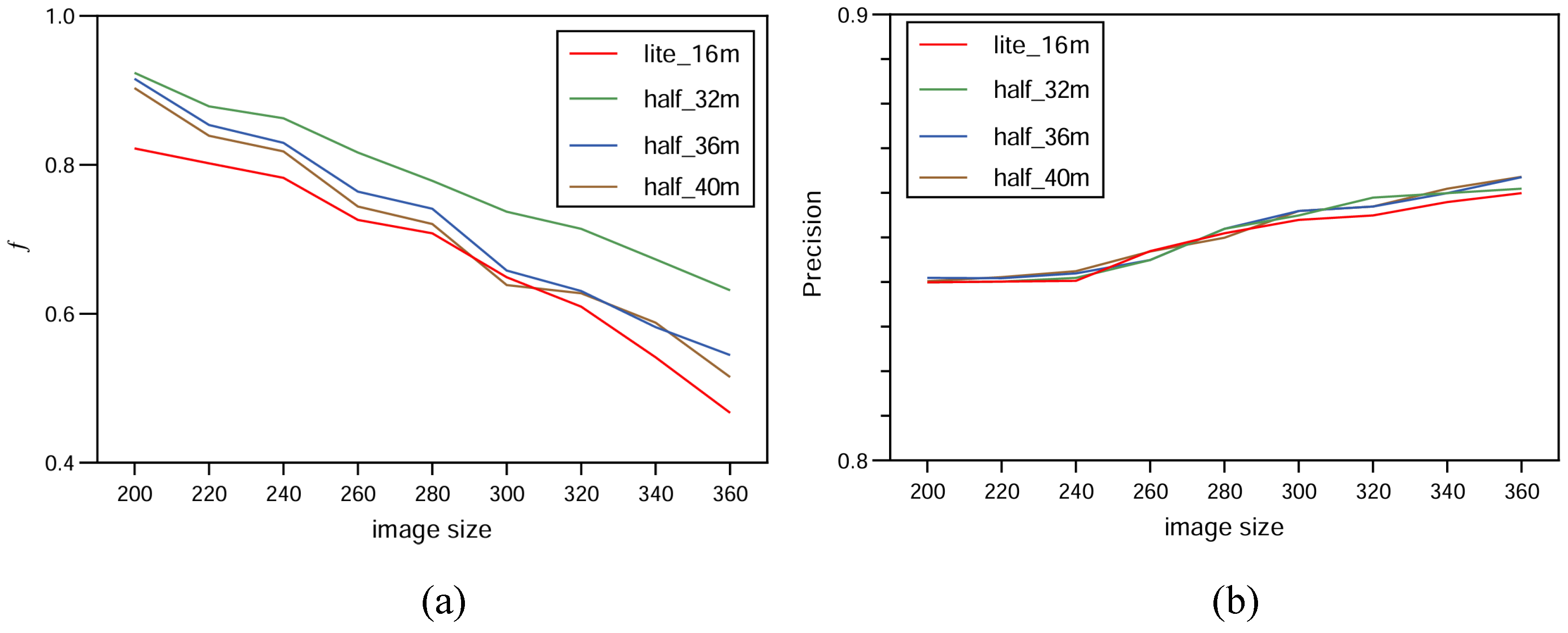
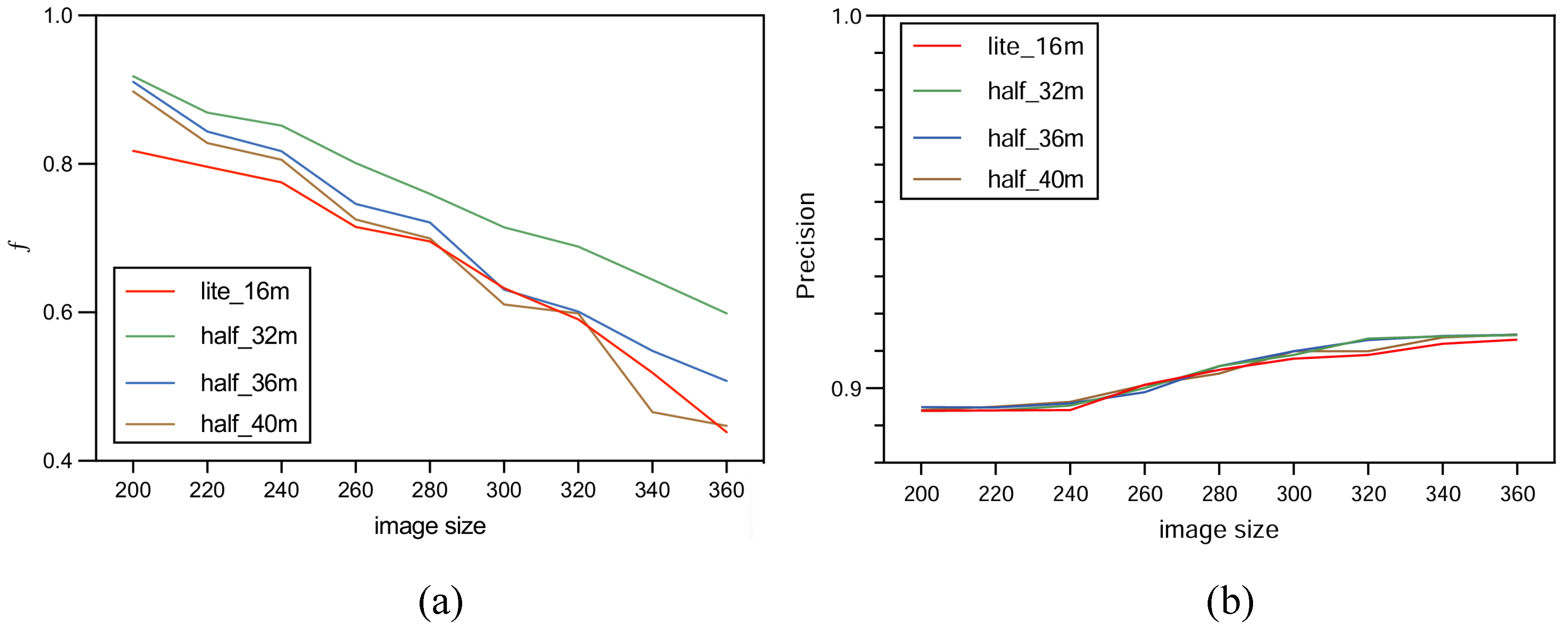
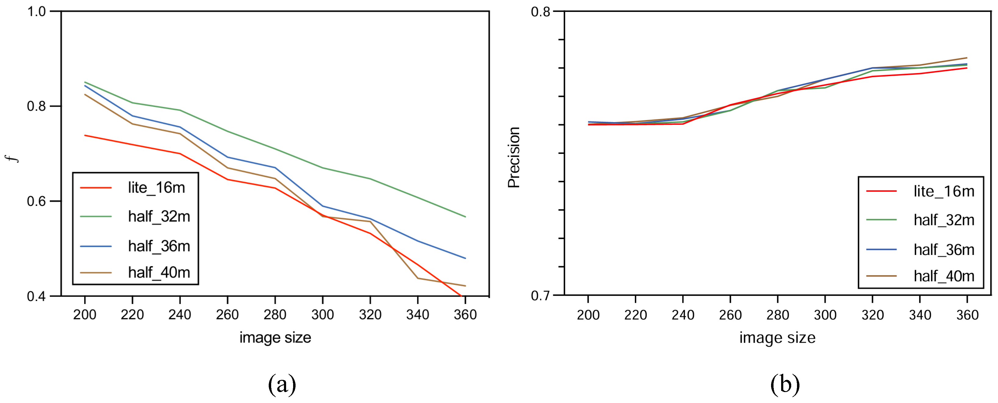
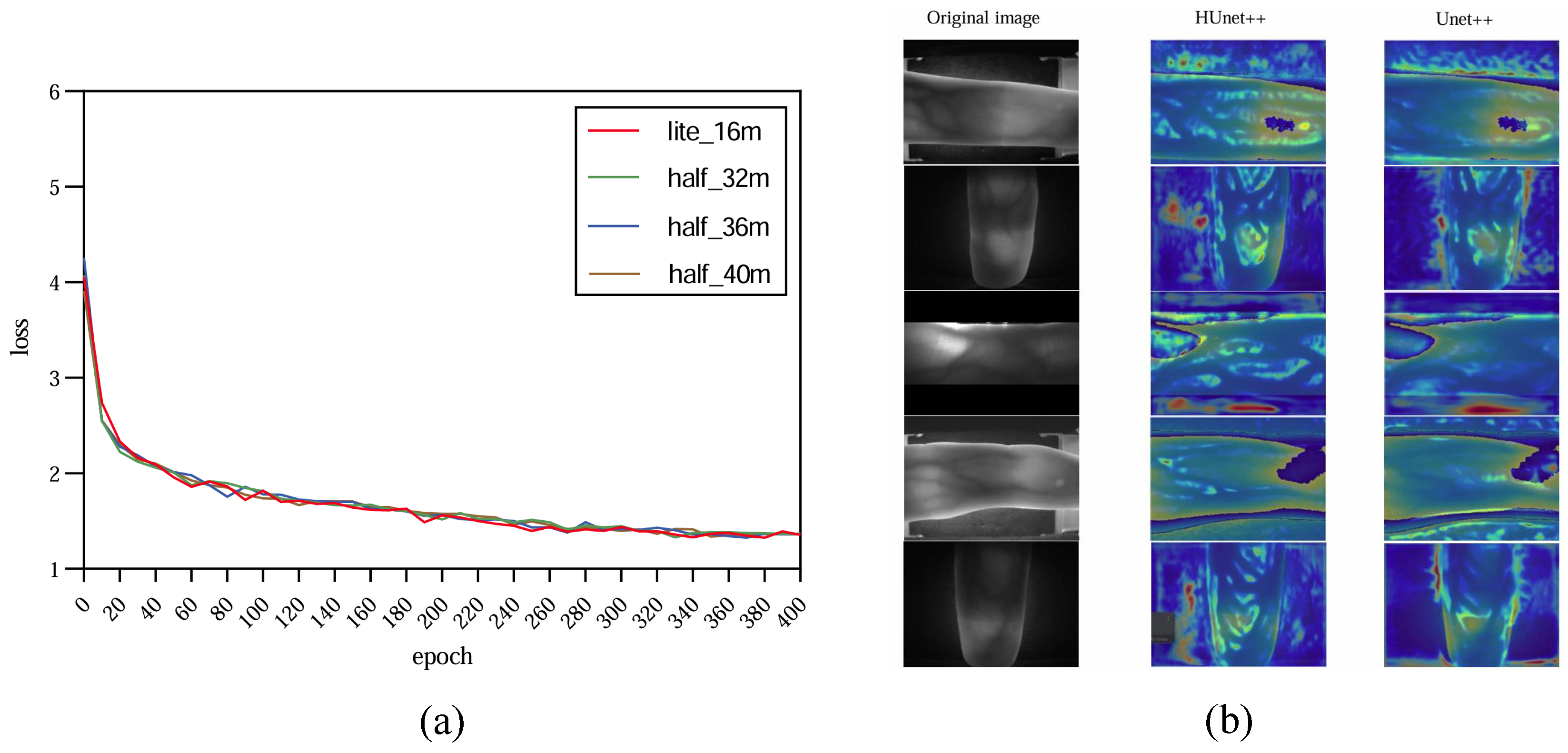
In order to increase confidence in the experiment, this study carried out multiple tests with HUnet++ and Unet++ on images of different sizes. Among these, HUnet++ was further divided into experiments with different hidden layers and compared with the lightweight version of Unet++. The final results are presented in the form of a line graph.

3.2. Data Preprocessing

The manual training set utilized in this study was formed by the fusion of three datasets, and manual annotation was conducted on the finger vein images within the combined dataset, comprising database of the University of Science, Malaysia (FV-USM) [30], the Shandong University dataset [31], and the self-built dataset (NCEPU-data). The composition of that dataset ensured the coverage of data with different sizes, lighting conditions, and resolutions, thereby further enhancing the model’s robustness. The training dataset included a total of 140 original images collected by finger vein devices and 140 annotated images corresponding to the original images, where the labels were binary images annotated manually. Out of these, 107 images were used for model training and the remaining 33 for testing the model. The specific processing workflow was as follows: Initially, all vein images were transformed into grayscale. Subsequently, based on the basis of the grayscale images, the vein regions were manually labeled as black (with a pixel value of 0), while the non-vein regions were designated as white (with a pixel value of 225). The aim of this preprocessing step was to minimize computational load during model execution by reducing the number of image channels. Before the model was trained, these images used for training and the labels used for model backpropagation underwent image normalization, data format conversion, and data augmentation operations. This then generated the data loader for subsequent model training.

For labels annotated using traditional finger vein extraction methods, five finger vein images were first generated using Gabor, MC, PC, RLT, and WLD techniques, with vein regions set to pixel value 1 and background to 0. These images were added element-wise to produce a fusion image, where elements with values >3 were set to 255, and others to 0. Formula (4) for fusing an image is shown below:

$$Fusion=Gabor+MC+2\times PC+RLT+WLD$$

(4)

Median blur and morphological opening were then applied to connect sparse vein regions, removing residual noise and enhancing the model’s ability to learn vein features. Figure 5 is the end result. During actual training, the vein region pixel values of all images were set to 0, while the background region was set to 255. This was carried out partly to maintain consistency with the manually annotated vein images and partly to ensure that the labels more closely resembled the original vein images. Based on the conclusions of Jalilian et al. [16] and the scale of the manually annotated dataset, we set the scale of all traditional-method-annotated finger vein datasets used for model training to be consistent with that of the manually annotated dataset.

The finger vein masks extracted using traditional methods contained both explicit geometric features and implicit non-geometric features (i.e., the non-geometrization and discontinuity of vein patterns). To optimize the model’s performance, we applied a weighting strategy during the training process on datasets annotated by traditional methods. This approach involved increasing the weight of the foreground region and decreasing the weight of the background region. For each dataset, the final weights for the foreground and background regions were determined through experiments, with the specific weights varying according to the characteristics of each dataset.

3.3. Model Parameter Configuration

The experiment was performed on the Google Colab platform with the following configuration: GPU: Tesla K80; RAM: 16 GB; operating system: Ubuntu 22.04.2 LTS; system memory: 12.7 GB; system kernel: 5.15.120+; disk space: 78.2 GB. The environment was set up with CUDA 12.0 and driver version 525.105.17. During the model training phase, experiments were conducted using three variations of the HUnet++ model, each with different numbers of hidden layers. In each experiment, the number of hidden layers in the convolutional layer of the encoding and decoding blocks of HUnet++ were 32, 36, and 40, respectively. Each experiment was conducted on nine different image sizes. Lastly, one experiment was conducted with the hidden layers of the Unet++ (lightweight) model set to 16. In that experiment, training comparisons were also made on nine different image sizes.

As illustrated in

Table 2. Parameter configuration of Unet++ and HUnet++ models (the structure of De_n and En_n in each model is identical, differing only in their parameters).

Module		Unet++	HUnet_32m	HUnet_36m	HUnet_40m
		hid,in,out	hid,in,out	hid,in,out	hid,in,out
Encoder	En_1	16,1,64	32,1,64	36,1,64	40,1,64
	En_2	16,64,64	32,64,64	36,64,64	40,64,64
	En_3	16,64,64	32,64,64	36,64,64	40,64,64
	En_4	16,64,64	32,64,64	36,64,64	40,64,64
	En_5	16,64,64	32,64,64	36,64,64	40,64,64
	En_6	16,64,64	32,64,64	36,64,64	40,64,64
Decoder	De_1	16,128,64	-	-	-
	De_2	16,128,64	-	-	-
	De_3	16,128,64	-	-	-
	De_4	16,128,64	-	-	-
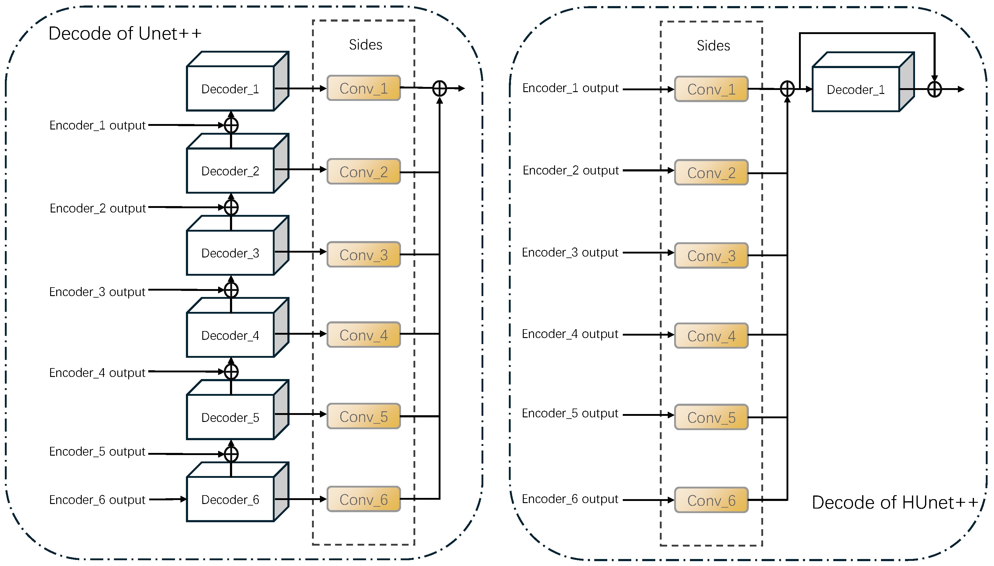
	De_5	16,128,64	32,6,64	36,6,64	40,6,64

, this study compared the parameter configurations of four models: Unet++, HUnet_32m, HUnet_36m, and HUnet_40m. In these models, the “hid, in, out” column represents the “hidden, input, output” of each module, and the “n” of En_n is the depth of each module. Specifically, in each of these models, the encoder component consisted of six En_n units. Regarding the decoder architecture, the Unet++ model included five De_n units, whereas the other three models contained only one De_5 unit.

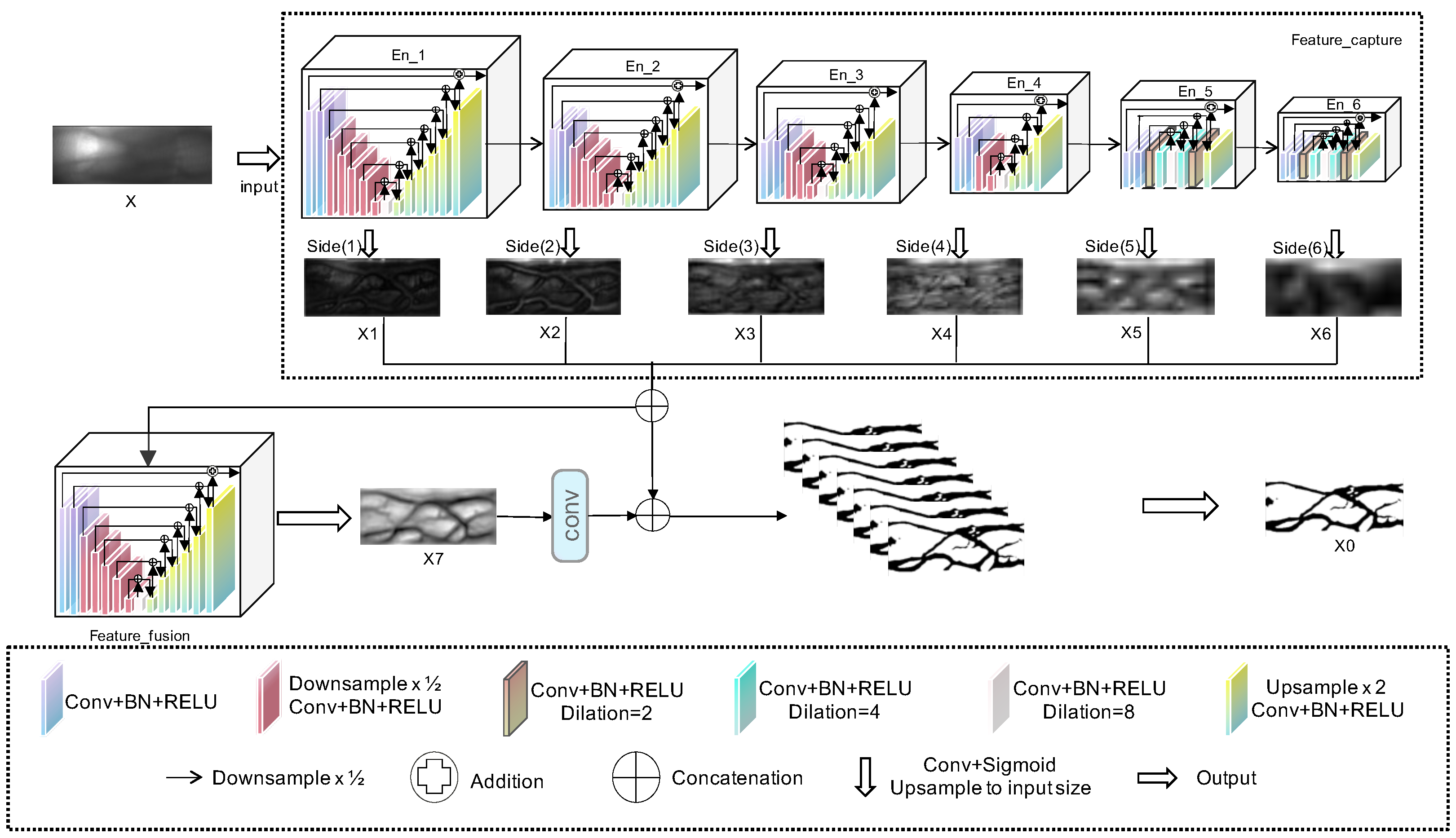
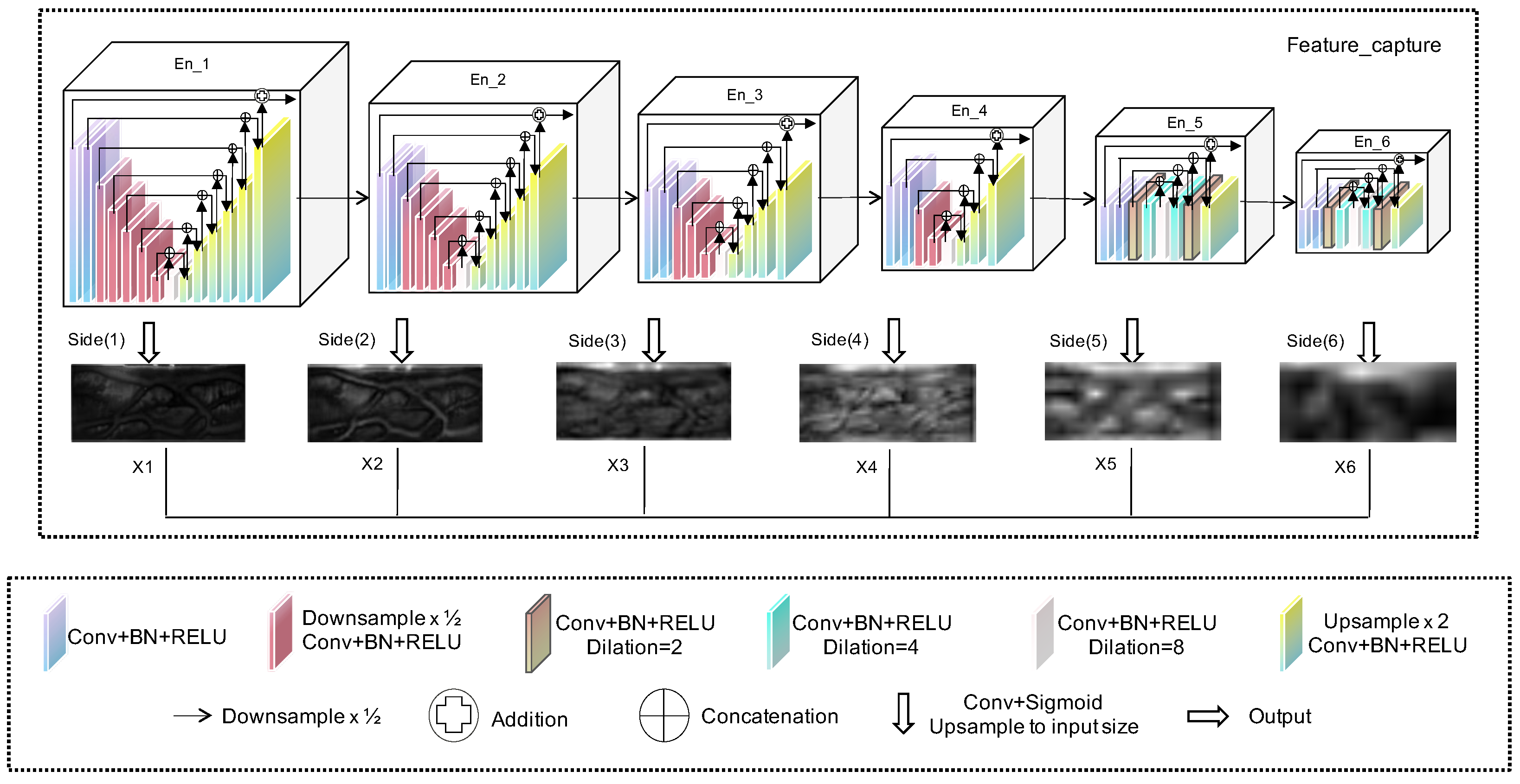
According to the data presented in Table 2, each En_n unit corresponds to the En_n shown in Figure 2. The De_5 unit corresponds to the Feature Fusion structure depicted in the same figure. Additionally, the structure of De_m (where m ranged from 1 to 4) was similar to that of its corresponding En_m (also ranging from 1 to 4), although their functions differed. Notably, in the three HUnet models, the decoder consisted solely of a De_5 unit. In contrast to the original Unet++ model, where the De_5 has an input channel of 128, in these models, the De_5 had an input channel of 6. This design was intended to integrate the finger vein features extracted by decoders at six different levels. Due to space constraints, this article uses the En_1 structure of the encoder in the HUnet++ model from Table 2 as an example to illustrate the significance of the En_n and De_n structure parameters detailed in Table 2.

Table 3. Parameter details for the En_1 structure within the encoder of the HUnet_32m model are provided.

Module		kernel,input,output	stride,padding	Dilation	BN (Input)	Relu
Encoder	conv_in	$3\times 3$,1,64	(1,1),(1,1)	-	64	✓
	encoder_1	$3\times 3$,64,32	(1,1),(1,1)	-	32	✓
	encoder_2	$3\times 3$,32,32	(1,1),(1,1)	-	32	✓
	encoder_3	$3\times 3$,32,32	(1,1),(1,1)	-	32	✓
	encoder_4	$3\times 3$,32,32	(1,1),(1,1)	-	32	✓
	encoder_5	$3\times 3$,32,32	(1,1),(1,1)	-	32	✓
	encoder_6	$3\times 3$,32,32	(1,1),(1,1)	-	32	✓
	encoder_7	$3\times 3$,32,32	(1,1),(2,2)	(2,2)	32	✓
Decoder	decoder_1	$3\times 3$,32,32	(1,1),(1,1)	-	32	✓
	decoder_2	$3\times 3$,32,32	(1,1),(1,1)	-	32	✓
	decoder_3	$3\times 3$,32,32	(1,1),(1,1)	-	32	✓
	decoder_4	$3\times 3$,32,32	(1,1),(1,1)	-	32	✓
	decoder_5	$3\times 3$,32,32	(1,1),(1,1)	-	32	✓
	decoder_6	$3\times 3$,32,64	(1,1),(1,1)	-	64	✓

elaborates on the parameter configuration of the En_1 unit within the encoder structure of the HUnet_32m model, as referenced in Table 2. Specifically, within the encoder structure of the HUnet_32m model in Table 2, the hidden, input, and output parameters of the En_1 unit are specified as (32, 1, 64). The input channels count corresponds to the input channels of the conv_in module within the encoder structure in Table 3. The output channels’ count aligns with the output channels of the last module, decoder_6, in the decoder structure of Table 3. The hidden layer parameters are consistent with the output channel numbers of all encoder_n units and all decoder_n units, except for decoder_6. Additionally, in Table 2, the depth associated with the En_1 unit in the encoder structure of HUnet_32m is 7, which corresponds to the highest number, encoder_7, in the encoder_n structure in Table 3. Across all En_n structures, the total number of decoder_n units is always one less than the total number of encoder_n units. Note that in all En_n structures, the convolutional layer in the final encoder_n module employs dilated convolution.

In the experiments involving the HUnet++ and Unet++ model, AdamW was adopted as the optimizer used throughout, with a weight-decay value of 1 $\times {10}^{-4}$. After training the models, the one with the best performance was compressed using the method of structural reparameterization. Structural reparameterization is a technique that enables the compression of model parameters while preserving accuracy, thus enhancing the model's prediction speed. This method typically involves merging convolution branches or convolution+BN blocks into a single convolution with an added bias term. To implement this, a new compressed model must be constructed, which, compared to the original model, only lacks the BN or convolution branch components. Afterward, the compressed weight file is loaded into the new model. The primary goal of this approach is to accelerate prediction, enabling real-time performance. In the experiments conducted in this study, the convolution+BN blocks were primarily compressed. The output of the matrix after passing through both the convolution block $wi$ and the BN block is equivalent to the output of a newly created convolution block $w{i}^{\prime }$ with an added bias term $\theta i$. As explained by Ding et al. [27], the value of the new convolution block $w{i}^{\prime }$ can be represented by Formula (5):

$${wi}^{\prime }=wi·{\displaystyle \frac{\gamma i}{\sqrt{\sigma i^2+ϵ}}}$$

(5)

The value of bias $\theta i$ is Formula (6):

$$\theta i=\beta i-{\displaystyle \frac{\mu i·\gamma i}{\sqrt{\sigma i^2+ϵ}}}$$

(6)

By substituting the original $wi$ and the weights of the BN layer with $w{i}^{\prime }$ and $\theta i$, the resulting model was compressed. Subsequently, the compressed model was evaluated against the original Unet++ (a lightweight variant of the Unet++ architecture) model for vein mask extraction on the test set, with a focus on comparing the extraction speed of vein masks between the two models.

4. Experiments and Results

4.1. Feature Extraction Diagram at Different Levels

Figure 6 clearly shows that the six encoders focused on extracting features at different levels. (a), (b), and (c) belong to shallow feature information, while (e), (f), and (g) belong to deep feature information. (d) is the result image after the feature fusion module combined the features of six different levels. The model balanced the feature maps at different levels, eliminating some unnecessary shallow features (such as fingerprints, uneven lighting, etc.) in the fused feature map, likely preserving the necessary venous network features of the vein.

4.2. Result of the Evaluation

4.2.1. Comparison Between the Original Model and the New Model

To validate the speed advantage of the proposed model in this paper, we performed training experiments on four models (original model: lite_16m, new model: half_nm) against nine different image sizes, and based on Formula (1), we plotted the line charts of the performance trends of several models as the image size increased.

In Figure 7, Figure 8, Figure 9 and Figure 10, in (a), “lite_16m” represents the Unet++ model with 16 hidden layers, “half_32m” represents the HUnet++ model with 32 hidden layers, “half_36m” represents the HUnet++ model with 36 hidden layers, and “half_40m” represents the HUnet++ model with 40 hidden layers. Since nearly half of the original model structure was removed, the initial number of hidden layers in the HUnet++ model was set to twice that of the original model (32 layers) based on our experimental results. Further experiments gradually increased the hidden layer count starting from that baseline.

From Figure 7a, it can be seen that the HUnet++ model with 32 hidden layers performed the best. From Figure 7b, it can be concluded that the overall precision of all models increased with the increasing image size after training on image data of different sizes. The difference in precision between models was within the range of −0.002 to 0.002, and the accuracy improved compared to the original model, but the effect was not very significant. Figure 8, Figure 9 and Figure 10 demonstrate similar effects, showing that, apart from the fact that the proposed model consumed less training time, the final training performance on the manually labeled dataset was superior to that on the dataset labeled by traditional methods. The training results across the four datasets demonstrated that the HUnet++ model with 32 hidden layers exhibited stable performance on all datasets. As the number of hidden layers increased, the final performance of the HUnet++ model gradually converged to that of the Unet++ model, particularly as the image size increased.

In

Table 4. Time for extracting vein mask from a single vein image(s).

Image Size (px)	200	220	240	260	280	300	320	340	360
Unet++	0.0252	0.0268	0.0264	0.0281	0.0291	0.0298	0.0299	0.032	0.0324
HUnet++	0.0118	0.015	0.0131	0.0142	0.0151	0.0168	0.0178	0.02	0.0218

, the prediction time per image for both models is also averaged across the four datasets, illustrating the models’ average prediction efficiency under varying dataset conditions.

Therefore, combining the comparisons of these aspects (Figure 7a–Figure 10a), this article ultimately adopted the HUnet++ model with 32 hidden layers as the model for the extraction of the vein mask and conducted structural reparameterization on that model. In Table 4, with a range of image sizes from 200 to 360 pixels, by comparing the time taken by the compressed HUnet++ and the original Unet++ model to extract the vein mask from a single image, it was found that the time for compressed HUnet++ to extract the vein mask was at least two-fifths of the time taken by the original Unet++ model, and at most two-thirds of the time taken by the original Unet++ model. Furthermore, the time consumed by the compressed HUnet++ model for image processing was between 0.01 and 0.02 s before the image pixel size reached 340, which was sufficient to meet real-time requirements for typical vein images.

Figure 11a shows the loss curves of the original model and the HUnet++ model with varying numbers of hidden layers. The results demonstrate that the proposed models achieved convergence speeds comparable to the original model, with negligible differences in their final loss values. During the training process, to prevent overfitting, all models incorporated the AdamW optimizer combined with a dynamic learning rate adjustment strategy. Such an approach allowed the models to undergo a learning rate warmup phase at the training’s initiation, followed by gradual adjustments throughout the training progression. This strategy effectively mitigated gradient oscillation issues caused by an excessively large initial learning rate and accelerated the convergence of the models.

Figure 11b shows the Grad-CAM [32] visualizations of the last decoding block for both the HUnet++ model (HUnet++ model with 32 hidden layers) and the original model. While both models effectively focused on finger vein regions, the Grad-CAM visualizations of HUnet++ demonstrates more precise activation areas, better highlighting the critical parts of the finger veins. However, HUnet++ was more susceptible to background interference compared to the original model. In contrast, the Grad-CAM visualizations of the Unet++ model display more dispersed attention in the finger vein regions while remaining unaffected by the background regions. These findings suggest that although the HUnet++ model demonstrated slightly lower robustness to background regions compared to the original model, it achieved superior performance in extracting and localizing vascular features within finger vein images.

4.2.2. Comparison Between the HUnet Model and Other Models

Six models, FCN [33] (the FCN_32s model was utilized here), Deeplab_v3 [29], LR_ASPP (MoblieNet_v3) [34], Unet [35], Unet++, and HUnet++, were trained on the dataset proposed in this paper, and three vein images were randomly selected for vein mask extraction. The extraction results are shown in Figure 12. During the training of the models, FCN, LR_ASPP, Deeplab_v3, and Unet utilized the SGD optimizer, while Unet++ and HUnet++ employed the AdamW optimizer. All models followed the same learning rate adjustment strategy during training, and the binary cross-entropy loss function was used for all models.

In order to make the comparison of the extraction results of various models more obvious, we thresholded the extraction result images output by the FCN, Deeplab_v3, LR_ASPP (MobileNetV3), and Unet models. The ultimate goal of extracting vein image masks for finger vein recognition is identity verification. Given the emphasis on speed and lightweight requirements, MobileNetV3’s advantages in mobile and edge computing devices align well with this purpose. Therefore, this study included MobileNetV3 in comparative experiments due to its efficiency in these scenarios. The lightweight Unet++ (Unet++_lite in the Figure 12) and HUnet++ models mapped all element values in the vein mask matrix output by the model to the range between 0 and 255. As seen in Figure 12, the effectiveness of different models for finger vein segmentation was analyzed under two distinct training scenarios: one where the labels were manually annotated (a), and the other where labels were derived using traditional vein extraction methods (b). The results demonstrated that the performance of the models varied notably depending on the type of labels used. When manually annotated labels were employed (a), models such as DeepLab_v3, Unet, Unet++ and HUnet++ showed relatively high consistency and detailed vein structure preservation, especially for complex vein patterns. In contrast, models like LR_ASPP and FCN exhibited noticeable discrepancies in some regions, possibly due to sensitivity to finer structural variations or inherent limitations in capturing vein intricacies. In scenario (b), where traditional extraction methods were used to generate labels, the overall segmentation quality showed a decline across most models. This was particularly evident in models such as Deeplab_v3, FCN, LR_ASPP and Unet, where the extracted vein masks tended to lose fine-grained details or introduce structural artifacts. This decline suggests that the noise or inaccuracies inherent in traditional labeling methods might propagate during model training, thereby affecting the final segmentation output. Nonetheless, some models, such as Unet++ and HUnet++, demonstrated better robustness in retaining vein patterns even under less accurate label conditions.

For the sake of objectivity, the final results of all models on different datasets presented in Figure 12 are summarized in

Table 5. Result of comparing the performance of our method on four datasets. Image size was 240 × 240. The unit of Pred is milliseconds (ms).

Model	Manually Annotated Dataset			SD_Data			FV_Data			CD_Data
	MaxF1	Pred	Precision	MaxF1	Pred	Precision	MaxF1	Pred	Precision	MaxF1	Pred	Precision
FCN	0.654	31.6	60.1%	0.791	28.7	79.9%	0.623	33.2	58.4%	0.853	27.3	81.7%
Deeplab	0.831	35.22	80.19%	0.767	36.17	73.36%	0.602	37.58	55.2%	0.795	35.93	74.92%
LR_ASPP	0.669	9.3	63.11%	0.799	9.94	75.94%	0.626	10.1	60.43%	0.855	9.4	79.12%
Unet	0.904	9.6	88.46%	0.826	10.2	78.96%	0.76	11.2	70.1%	0.871	9.7	82.7%
Unet++	0.948	26.4	91.4%	0.894	29.9	84.03	0.825	30.1	78.09%	0.93	27.1	89.4%
HUnet++	0.946	13.1	91.4%	0.895	13.3	84.1%	0.824	13.1	78.07%	0.933	12.9	89.5%

. The Manually Annotated Dataset corresponds to (a) in Figure 12, while FV_data, SD_data, and CD_data correspond to the three rows of images in (b), from top to bottom.

In Table 5, Pred represents the time the model required to predict a single image on the dataset. Table 5 provides the forecast time, $MaxF1$, and precision for the six models. In terms of the time taken to extract a vein mask, the LR_ASPP model was the fastest. Its performance on datasets annotated using traditional methods surpassed that on manually annotated datasets, but the results were highly susceptible to image quality. Moreover, it is evident from the result that the FV_data dataset exhibited the poorest performance among all datasets. This may be attributed to the lower image quality and the coexistence of two different image formats within the dataset. However, the HUnet++ model achieved higher precision while only on average being 0.00317 s slower than the LR_ASPP model in prediction time across the four datasets. Looking at the training speed, the HUnet++ model improved upon the speed of the lightweight Unet++ model. The data in Table 5 also reveal that the Unet++ and HUnet++ models outperformed the other models on each dataset.

In

Table 6. Comparison of model parameters between Unet++ and HUnet++.

Model	Total Params	Total Memory	Total MAdd	Total Flops	Total MemR+W
Unet++	4.3 MB	1.34 GB	22.4 GMAdd	11.21 GFlops	803.71 MB
RUnet++	4.28 MB	961 MB	22.16 GMAdd	11.09 GFlops	621.78 MB
HUnet++	4.31 MB	1.16 GB	18.43 GMAdd	9.22 GFlops	797.13 MB
RHunet++	4.29 MB	833 MB	18.23 GMAdd	9.11 GFlops	615.16 MB

, RUnet++ refers to the Unet++ model compressed using the structural reparameterization method, while RHUnet++ refers to the HUnet++ model compressed with the same method. As can be clearly seen from the Table 6, the proposed model in this paper showed reductions in model parameters, total memory size, and total MemR+W compared to the original Unet++ model. Furthermore, after structural reparameterization, the proposed model achieved a more significant reduction in these metrics compared to the original model. In comparison to the direct structural reparameterization of the Unet++ model, the proposed model demonstrated superior performance after reparameterization.

4.3. Discussion

Although Unet-series models perform excellently in vascular feature extraction and are widely used in medical image processing, their main challenge in real-time recognition tasks lies in efficiency and lightweight design. In order to resolve this problem, we proposed the HUnet++ model based on the Unet++ architecture and conducted a series of experiments using that model.

In the analysis of the results (

Table 7. Result of comparing the performance of our method on four datasets. Image size was 240*240. The unit of Pred is milliseconds.

Model	Params	Manually Annotated Dataset		SD_Data		FV_Data		CD_Data
		Pred	Precision	Pred	Precision	Pred	Precision	Pred	Precision
FCN	35.3 MB	0.316 s	60.1%	0.287 s	79.9%	0.332 s	58.4%	0.273 s	81.7%
Deeplab	41.98 MB	0.352 s	80.19%	0.362 s	73.36%	0.376 s	55.2%	0.359 s	74.92%
LR_ASPP	3.22 MB	0.093 s	63.11%	0.099 s	75.94%	0.101 s	60.43%	0.094 s	79.12%
Unet	4.32 MB	0.096 s	88.46%	0.102 s	78.96%	0.112 s	70.1%	0.091 s	82.7%
Unet++	4.3 MB	0.264 s	91.4%	0.299 s	84.03%	0.301 s	78.09%	0.271 s	89.4%
HUnet++	4.29 MB	0.131 s	91.4%	0.133 s	84.1%	0.131 s	78.07%	0.129 s	89.5%

), we observed that different methods of vein annotation had varying impacts on model performance. In this study, vein images annotated using traditional methods tended to have scattered vein region pixels and contained more noise, which led to poorer model performance on the traditional-method-annotated dataset compared to the manually annotated dataset. On the other hand, the final extracted vein masks clearly showed that the Unet-series models outperformed other models. As for the LR_ASPP model, it demonstrated significant advantages over other models in terms of prediction speed and memory consumption. Moreover, the vein masks extracted from all datasets except the FV_data dataset exhibited a linear distribution, indicating that the LR_ASPP model still holds potential for further research and optimization in the field of vein feature extraction and recognition.

Additionally, the approach proposed in this study demonstrated that appropriate pruning and increasing the number of hidden layers could reduce model training time while maintaining accuracy. This provides an effective way to lower the cost of the model training process.

In our study, we found that although the finger vein masks generated from manually annotated datasets exhibited better geometric performance compared to those annotated using traditional methods, this alone was not sufficient to prove that manually annotated datasets outperformed traditional-method-annotated datasets in finger vein recognition. To comprehensively compare the advantages and disadvantages of the two approaches, more experiments focused on finger vein mask-based recognition are necessary. Furthermore, we recognize that if both annotation methods have their respective strengths, it is worth exploring whether there exists a way to effectively integrate the final results from both methods. This remains a direction for further research and investigation. In addition to referencing methods related to vein segmentation, we also paid attention to studies on path and curve segmentation. We believe that our approach may also have potential applications in these areas.

5. Conclusions

In this study, we first manually annotated 140 finger vein images to construct a training dataset containing vein masks. After annotation, we performed cross-validation by multiple annotators to verify the labels, ensuring the dataset’s validity and reliability. Subsequently, we employed five traditional finger vein feature extraction methods to extract features from two publicly available datasets and our custom-built dataset. Finally, by performing a weighted sum of the finger vein masks (with pixel values of zero or one) obtained from the five methods, a mask with a weighted sum greater than or equal to three was considered as the final finger vein mask extracted using traditional methods. The experimental results demonstrated that the proposed model performed excellently on datasets with both annotation methods and outperformed other models in terms of finger vein mask extraction speed.

In terms of model performance evaluation, we considered not only precision but also prediction speed, and we assessed the performance of various models using a weighted value method. The higher the value of the performance evaluation function f defined in this study, the better the model’s performance. This approach consolidated multiple evaluation metrics into a single function f, facilitating an intuitive comparison of model efficacy and thus clarifying the comparison among different models.

Based on the Unet++ model, this paper proposed the HUnet++ approach, which was experimentally validated to improve training speed across images of various sizes. After training the HUnet++ model with different numbers of hidden layers, experimental results indicated that the HUnet++ model with 32 hidden layers exhibited the best comprehensive performance in terms of trend changes, training duration, and accuracy. We employed structural reparameterization to compress the model with 32 hidden layers, significantly enhancing the speed of finger vein mask extraction. Consequently, we selected the HUnet++ model with 32 hidden layers as the tool for extracting finger vein masks. After structural reparameterization, the model demonstrated that the speed of extracting vein masks from common-sized finger vein images was at least 1.5 times faster than the lightweight Unet++ original model, with actual processing times ranging from 0.01 to 0.024 s, the proposed method achieved precision rates of 91.4%, 84.1%, 78.07%, and 89.5% on the manually labeled dataset and the traditionally labeled datasets (SDUMLA-HMT, FV-USM, Custom dataset), sufficiently meeting real-time processing demands. Therefore, the method proposed in this paper not only preserved the accuracy of the original model in finger vein feature extraction but also significantly improved the model’s training speed and the feature extraction speed for individual images. The only limitation was that the finger vein masks generated from manually annotated datasets exhibited better geometric performance compared to those annotated by traditional methods, so more experiments are still needed to determine which one performs better in recognition tasks. Our research achieved efficiency optimization and model compression for high-precision models, providing new insights for the field of finger vein recognition. Furthermore, it holds significant importance for the implementation of real-time recognition tasks across various devices and the exploration of applications in related domains.