A Hybrid Tree Convolutional Neural Network with Leader-Guided Spiral Optimization for Detecting Symmetric Patterns in Network Anomalies

Abstract

In the realm of cybersecurity, detecting Distributed Denial of Service (DDoS) attacks with high accuracy is a critical task. Traditional machine learning models often fall short in handling the complexity and high dimensionality of network traffic data. This study proposes a hybrid framework leveraging symmetry in feature distribution, network behavior, and model optimization for anomaly detection. A Tree Convolutional Neural Network (Tree-CNN) captures hierarchical symmetrical dependencies, while a deep autoencoder preserves latent symmetrical structures, reducing noise for better classification. A Leader-Guided Velocity-Based Spiral Optimization Algorithm is proposed to optimize the parameters of the system and achieve better performance. A Leader-Guided Velocity-Based Spiral Optimization Algorithm is introduced to maintain a symmetrical balance between exploration and exploitation, optimizing the autoencoder, Tree-CNN, and classification thresholds. Validation using three datasets—UNSW-NB15, CIC-IDS 2017, and CIC-IDS 2018—demonstrates the framework’s superiority. The model achieves 96.02% accuracy on UNSW-NB15, 99.99% on CIC-IDS 2017, and 99.96% on CIC-IDS 2018, with near-perfect precision and recall. Despite a slightly higher computational cost, the symmetrically optimized framework ensures high efficiency and superior detection, making it ideal for real-time complex networks. These findings emphasize the critical role of symmetrical network patterns and feature selection strategies for enhancing intrusion detection performance.

1. Introduction

The rapid evolution of network technologies and the exponential growth in the number of internet-connected devices have led to a sharp increase in cyber threats [1]. Among these, Distributed Denial of Service (DDoS) attacks have risen to become one of the most frequent and destructive challenges. They can severely impact critical infrastructure and disrupt services, thereby making the detection of such attacks with high accuracy and reliability a critical component of network security [2]. However, the traditional approaches of machine learning fail to address the issues of the high-dimensionality, complexity, and dynamic nature of network traffic data effectively. It is, therefore, required to develop novel frameworks that can extract attack-specific symmetrical patterns, reduce noise, and adaptively detect anomalies with precision.

DDoS attacks can be categorized into various types, and each attack targets specific network query patterns. The main categories are volumetric attacks, which attack the available network bandwidth; protocol attacks, which target servant’s resources; application layer attacks, that target resources at the application level; amplification attacks, that take advantage of protocols to multiply incoming traffic; and low-and-slow attacks that use restricted bandwidth but target weakness [3]. However, volumetric and resource consumption DDoS attacks are more disruptive as they overwhelm network and server resources on a large scale, thus making them harder to detect and mitigate quickly. Because of their ease of execution, they are more prevalent than application layer attacks. Thus, our study focuses on both types of attacks and seeks to offer a promising solution.

It is known that simple statistical methods are inappropriate in describing different attack characteristics, and many of the systems show high false-positive rates, especially for low-intensity attacks [4]. Also, traditional methods do not have the edge of the real-time processing involved in high-speed networks. Thus, they are inappropriate for addressing large-volume or high-speed modern DDoS attacks threatening an organization’s server. The methods based on deep learning provide practical solutions to these challenges. Hence, these advanced techniques are thus very flexible, enabling them to learn patterns from the data and classify new attack types without being hard-coded. Deep learning models can handle large volumes of data and offer near-real-time responses due to the availability of appropriate hardware [5]. In addition, these models are capable of learning continuously; they can update themselves in real time based on shifting state and attack patterns. However, these approaches also possess some limitations, such as a lack of dynamic feature adaptation, which hinders their ability to monitor the varying attack patterns, and the absence of a multi-instance learning framework, which leads to suboptimal decision-making when handling complex, multi-faceted network traffic data [6].

One of the most critical challenges in DDoS attack classification is the huge volume and asymmetric nature of the query patterns that are generated in the course of an attack. Networks under DDoS attacks are flooded with gigantic volumes of traffic, making it challenging for traditional security systems to process and analyze the data in a real-time manner [7]. This high data volume complicates real-time monitoring while straining computational resources, requiring more-efficient and scalable solutions. This brings forth yet another complexity arising from the fact that DDoS attacks evolve and change; they keep changing. Since they continuously modify their ways to go unseen, they engage in obfuscating their traffic and also in spoofing [8]. Due to this aspect, classifiers need to learn adaptability to new changes; thus, a new change requires continuous modification, updating and refining detection models. This dynamic aspect makes static detection methods inadequate, highlighting the need for adaptive and flexible classification systems.

Class imbalance poses another critical challenge. When normal traffic dominates the traffic sample while attack traffic becomes relatively infrequent, creating a skew that impacts overall classification model performance, things become tricky. A learning model developed from such data might over-represent the dominating class, thereby causing an inferior detection rate of classes that appear less frequently, like various attack types. The need for proper identification and classification requires creating balanced models. With more challenging adversarial attacks that bring in further difficulties towards solving the DDoS classification problem, an adversary may deploy misleading and confusing techniques, creating techniques to fool and puzzle detection algorithms and evading being detected based on the exploitation of the models’ vulnerability. Such manipulative strategies may produce false negatives or lower the accuracy of detection, which shows the requirement for strong models that could resist such attacks [9]. The potential for the detection and opposition of adversarial attacks helps maintain the reliability and effectiveness of the classification systems.

The main goal of this work is to propose a new anomaly detection framework that can greatly improve attack detection rate with a balanced time complexity. To this end, we set the following goals: (1) hierarchical multi-scale feature extraction to learn high-granularity network traffic patterns, (2) compact latent learning for effective noise-free representation, and (3) hybrid optimization strategies for the best parameter tuning and enhanced model efficiency. In order to achieve these goals, we propose a Tree Convolutional Neural Network (T-CNN) that mines multi-scale hierarchical features, which allows for the detection of subtle anomalies easily missed by traditional models. A deep autoencoder also learns low-dimensional noise-free latent codes from high-dimensional data, efficiently denoising and retaining significant patterns for higher classification accuracy.

To further refine performance, we integrated a Leader-Guided Velocity-Based Spiral Optimization Algorithm that maximizes exploration–exploitation by merging the strength of the Pelican Optimization Algorithm and Particle Swarm Optimization. A hybrid method allows for optimal parameter tuning of the system, with improved model efficiency without the imposition of high time complexity. Additionally, an ensemble metaclassifier is introduced to aggregate predictions from multiple models, increasing robustness and generalizability in anomaly detection tasks. The proposed method has been rigorously tested on three benchmark datasets, namely UNSW-NB15, CIC-IDS 2017, and CIC-IDS 2018. Comparative analysis with state-of-the-art techniques demonstrates that the framework can gain superior accuracy, precision, recall, and F1 scores for all the datasets. These results confirm the robustness and adaptability of the proposed methodology for various network security scenarios.

Our contribution can be summarized by the following points:

• We introduced a hierarchical T-CNN architecture that extracts multi-scale features from network traffic. It allows for the detection of slight anomalies that other models may miss. This architecture improves the granularity of features for better detection accuracy.
• We used a deep autoencoder to learn compact, noise-free latent representations of high-dimensional network data, thereby reducing data noise while keeping important patterns for classification and highly boosting the quality of feature representation towards anomaly detection.
• A hybrid optimization technique was developed, which combined the strengths of exploration by the Pelican Optimization Algorithm and exploitation by Particle Swarm Optimization. It enhanced the fine-tuning of system parameters and improved model efficiency. Optimization enhances adaptability across various network scenarios.
• We integrated an ensemble metaclassifier to aggregate predictions from multiple models, which improved robustness. It reduced overfitting and enhanced generalizability, especially in imbalanced datasets. It ensured consistent performance across different anomaly detection tasks.
• We validated the framework on the UNSW-NB15, CIC-IDS 2017, and CIC-IDS 2018 datasets. The comparison analysis indicated better accuracy, precision, recall, and F1-score. This validated the robustness and scalability of the framework in multiple network environments.

This paper is organized as follows. Section 2 discusses current anomaly detection and optimization methods, their shortcomings, and the necessity for enhancement. Section 3 introduces the proposed framework, explaining the Tree-CNN for multi-scale feature learning, the autoencoder for noise-free latent learning, and the Leader-Guided Velocity-Based Spiral Optimization for effective parameter tuning. Section 4 explains the experimental setup, dataset choice, benchmarking, and comparative analysis, proving the framework’s better performance. Lastly, Section 5 presents the main conclusions, addresses practical implications, and defines avenues for future research.

2. Related Work

This section presents the existing works related to this domain, specifying the methods used, the results attained, the accuracy achieved, and the drawbacks (See

Table 1. A summary of a few recently published articles on DDOS detection.

Index	Reference	Limitations Addressed	Proposed Methodology	Limitation
1	Yin et al. (2018) [10]	Lack of scalability in low-resource environments	DDoS detection in IoT using cosine similarity	Unsuitable for low-resource environments
2	Khatri et al. (2023) [11]	Poor performance on real cloud traffic	ANN-based DDoS detection in cloud environments	Struggles with dynamic cloud traffic
3	Parmar et al. (2023) [12]	Complexity of metric used for anomaly classification	Sequential autoencoder for anomaly detection	Complex metric limits distinction between benign and DDoS traffic
4	Wang et al. (2023) [13]	Limited to specific attack types, lacking generalizability to new patterns	Multi-scale CNN for multilevel DDoS detection	Limited novelty
5	Bala and Bahal (2024) [14]	Analysis of multiclass DDoS classification in IoT	Systematic review of AI-based IoT DDoS approaches	Limited studies involved
6	Hnamte et al. (2024) [15]	Applicability and scalability of DDoS detection on real-world datasets	Scalable DNN framework for analyzing network traffic	High applicability but needs testing in other real-world datasets
7	Anley et al. (2024) [16]	Limited to binary and multi-label DDoS classification	Customized CNN and pre-trained architectures for DDoS detection	Limited to specific types of classification tasks
8	Zhao et al. (2023) [17]	Struggles with scaling data size and learning novel attack patterns	CNN–Bidirectional LSTM to preserve spatial and temporal data characteristics	Issues with large data sizes and new attack paradigms
9	Presekal et al. (2023) [18]	Limited performance comparison across other architectures	Hybrid GC-LSTM and deep CNN for time-series-based anomaly detection	Lacked robustness across diverse datasets
10	Aktar and Nur (2024) [19]	No dynamic adaptation to evolving attack patterns	Contractive autoencoder-based anomaly detection	Performance limited to specific datasets
11	Jiyad et al. (2024) [20]	Limited generalization for unknown attack categories	Synthetic oversampling with ensemble learning	Poor performance to unknown attacks
12	Qaddos et al. (2024) [21]	Hybrid CNN-GRU model combined with FW-SMOTE to address imbalanced datasets.	IoTID20 and UNSW-NB15	Achieved 99.60% accuracy on IoTID20 and 99.16% accuracy on UNSW-NB15.
13	Sajid et al. (2024) [22]	Integrated XGBoost and CNN for feature extraction, combined with LSTM for classification.	CIC IDS 2017, UNSW-NB15, NSL KDD, and WSN-DS	Achieved binary and multiclass classification with optimized feature spaces
14	Ye et al. (2024) [23]	Enhanced HBO-based feature selection with Levy flight and Elite (LE) opposition-based learning strategies.	CEC2021, UCI, NSL-KDD, WUSTL-IIOT, and HAI	Improved feature selection for intrusion detection
15	Kumar et al. (2024) [24]	Authors implemented Deep Residual Convolutional Neural Network and Improved Gazelle Optimization Algorithm to improve local search ability of anomaly detection process and improve accuracy.	UNSW-NB-15, Cicddos2019, and CIC-IDS-2017 datasets	Parameter-sensitive model; scope of maximizing accuracy levels on both datasets.

).

A DDoS application was developed using deep learning in detection, presented by Yin et al. (2018) [10], who discussed an algorithm for DDoS attack detection and elimination using the Software-Defined IoT framework by considering the cosine similarity of vectors and defining threshold values for cosine similarity and vector length. Still, in terms of addressing the pinpointed problem, their model required intensive computational resources and was quite hard to execute easily in free-resource environments. Khatri et al. (2023) [11] diagnosed DDoS attacks using an artificial neural network in the cloud environment. However, when their approach was directly applied to real cloud traffic, outcomes demonstrated poor performance with the dynamic nature of the C2C traffic plus the varieties of services in run-on cloud infrastructures. Parmar et al. (2023) [12] introduced the method of a sequence-to-sequence autoencoder without any supervision in the context of anomaly detection of network traffic. Their method showed promise in revealing as-yet-unknown patterns of attacks. However, there were some issues associated with it because of the difficulty of using the metric adopted to classify traffic anomalies as benign or a real DDoS. Wang et al. (2023) [13] developed a novel Multi-Scale Convolutional Neural Network (MS-CNN) for the detection of DDoS attacks. They extracted multi-scaled features from the network traffic for the recognition of various levels of attack aggressiveness and length. The MS-CNN achieved an accuracy of 99.3% on the ISCX2012 dataset.

Bala and Bahal (2024) [14] systematically reviewed several research papers on AI-based tools and techniques used to analyze, classify, and detect IoT-based DDoS attacks between 2019 and 2023. This study recapitulated the performances of various ML/DL techniques on various skewed/imbalanced datasets in multiclass DDOS attack classification. Hnamte et al. (2024) [15] proposed a new DNN-based method for DDoS attack detection, with the analysis of network traffic data performed using a scalable and adaptive framework. The high applicability of this method was demonstrated by experiments on real-world datasets, where it achieved average accuracy rates of 99.98%, 100%, and 99.99% on the InSDN, CICIDS2018, and Kaggle DDoS datasets, respectively. Anley et al. (2024) [16] proposed three customized CNN DL architectures to test one-dimensional input vectors, namely (i) Conv4 (4 Layers), (ii) Conv8 (8 Layers), and (iii) Conv18 (18 Layers), and three pre-trained models, namely VGG16, VGG19, and ResNet50. For each architecture, the authors tested binary classification, separating benign traffic from DDoS attacks, and multi-label classification, identifying various attack types.

Zhao et al. (2023) [17] introduced a CNN–Bidirectional LSTM for DDoS attack identification. The authors further observed that the performance of his model exhibited capability towards keeping both the spatial and temporal properties of network traffic, but could not deal with data size and learning new paradigms about an attack. Furthermore, Presekal et al. (2023) [18] presented an architecture called the hybrid Graph Convolutional Long Short-Term Memory (GC-LSTM) model and a deep convolutional network for time-series-classification-based anomaly detection. From the presented comparison result, it follows that the classification accuracy, precision, recall, and F1 score obtained were in favor of the suggested hybrid model when compared to four traditional models; these were, namely, as follows: (1) ResNets, (2) Inception, (3) Fully Connected Network (FCN) [19], and (4) the Fully Connected Perceptron MLP models. Aktar and Nur (2024) [19] proposed a deep learning-based anomaly detection method based on a contractive autoencoder, which learned the normal traffic pattern and applied stochastic threshold for attacks. It was evaluated against the CIC-IDS2017, NSL-KDD, and CIC-DDoS2019 datasets. Compared with a simple autoencoder and other deep learning methods, it remarkably outperformed them, showing accuracy scores of 93.41–97.58% on CIC-DDoS2019, 96.08% on NSL-KDD, and 92.45% on CIC-IDS2017. Jiyad et al. (2024) [20] proposed a novel synthetic oversampling technique with ensemble learning. Experimental results showed that their method improved the identification of minority attack classes while suffering from generalization for the other unknown attack categories.

Qaddos et al. (2024) [21] introduced an innovative approach combining the structures of a CNN and GRU for IoT intrusion detection. This hybrid model can capture high-level features and learn important relational aspects that are more critical for IoT security. Moreover, FW-SMOTE is used to solve one of the major problems arising in intrusion detection tasks related to imbalanced datasets. Testing it on the IoTID20 dataset, a benchmark specially designed to emulate the real IoT environment with high efficiency, the model achieved an attack detection accuracy of 99.60%, overtaking previously existing benchmarks. Additionally, testing on the UNSW-NB15 network domain dataset showed good performance, achieving an accuracy of 99.16%. Sajid et al. (2024) [22] integrated Extreme Gradient Boosting (XGBoost) with convolutional neural networks (CNNs) for feature extraction, followed by integration with Long Short-Term Memory (LSTM) networks for classification purposes. This work used four benchmark datasets-CIC IDS 2017, UNSW NB15, NSL KDD, and WSN DS-to train models for binary and multiclass classification. Ye et al. (2024) [23] presented a novel ensemble framework for intrusion detection that stands out by virtue of its feature selection enhanced by an improved Hybrid Breeding Optimization method. Modifications on the Levy flight and Elite (LE) opposition-based learning strategies of the essential Hybrid Breeding Optimization (HBO) have been made to enhance the searching ability for higher performance. Furthermore, for more optimal FS in intrusion detection settings, a Cooperative Co-evolution Improved HBO framework has been put forward, where features are ranked and grouped based on data samples, subpopulations of LE-HBO of an appropriate size are assigned to each feature space, and the best feature subset is found through collaborative cooperation among the subpopulations. Kumar et al. (2024) [24] proposed a framework for intruder detection system optimization through the Deep Residual Convolutional Neural Network (DCRNN), in which further enhancement was gained by the Improved Gazelle Optimization Algorithm (IGOA). The selection of key features was executed by the Novel Binary Grasshopper Optimization Algorithm (NBGOA). Experiments were executed with datasets UNSW-NB-15, Cicddos2019, and CIC-IDS-2017, reporting improved statistical results compared to various baselines.

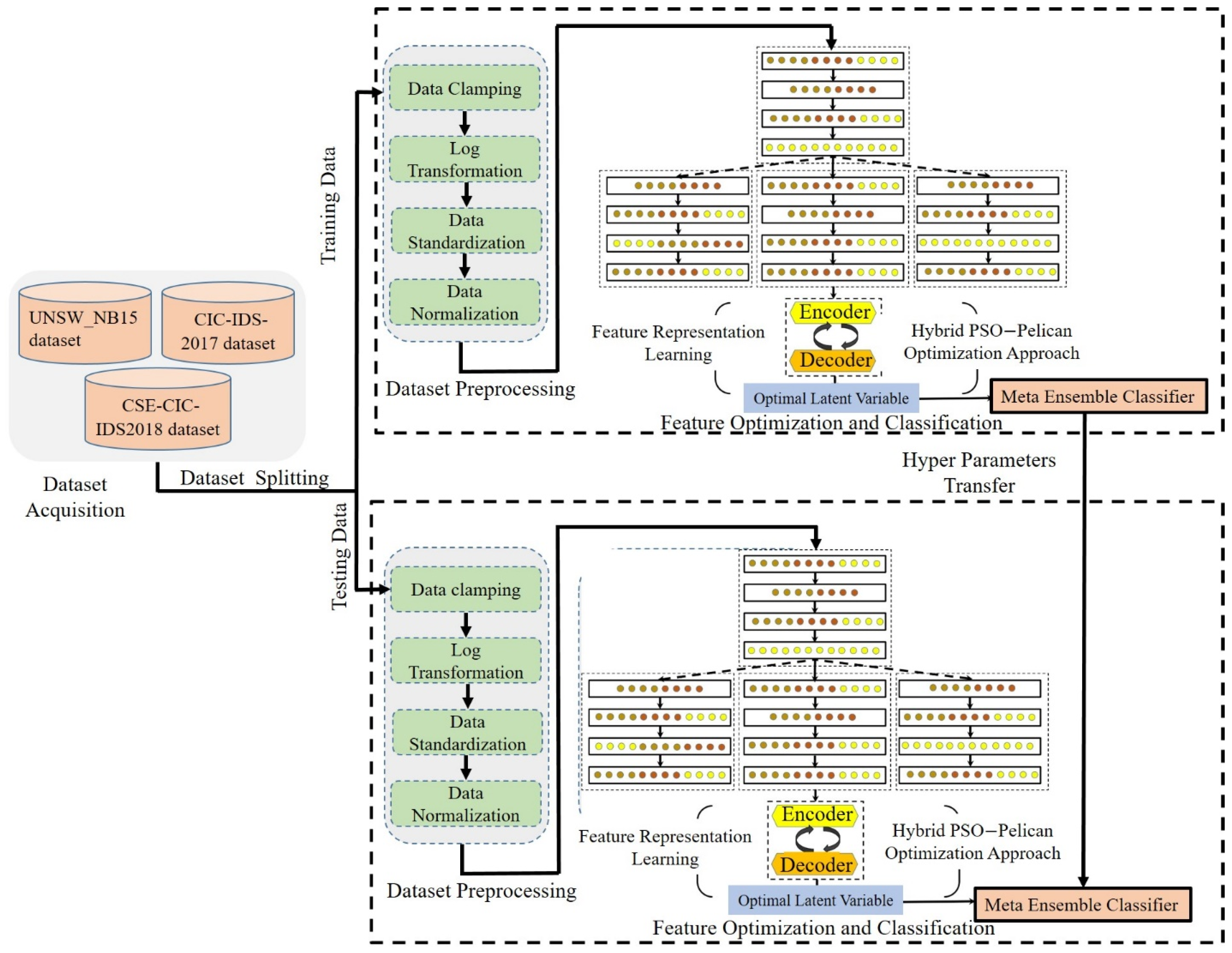
3. Proposed Methodology

This section is divided into three subsections: data collection, model construction, and, finally, the assessment of the model. Data preparation looks to improve the quality of the data and decrease the running time of the model. Figure 1 depicts the working pipeline of the proposed methodology. In the following subsections, we briefly explain how each step works and propose the architecture of our DDOS attack detection and classification network.

3.1. Data Collection

Three standard datasets—(1) UNSW_NB15 [25], (2) CIC-IDS-2017 [26], and (3) CSE-CIC-IDS2018 [27]—were employed in this paper to ensure the effectiveness of DDoS attack detection utilizing the developed advanced hierarchical neural network structure, which incorporates a new deep autoencoder with metaheuristics to generate discriminative results.

3.1.1. UNSW_NB15 Dataset

The raw network packets of the UNSW-NB 15 dataset were created by the IXIA Perfect Storm tool in the Cyber Range Lab of UNSW Canberra to generate a hybrid of real modern normal activities and synthetic contemporary attack behaviors. The tcpdump tool captured 100 GB of raw traffic (e.g., Pcap files). This dataset has nine types of attacks: Fuzzers, Analysis, Backdoors, DoS, Exploits, Generic, Reconnaissance, Shellcode, and Worms. The Argus and Bro-IDS tools were used, and twelve algorithms were developed to generate 49 features with the class label. These features are described in the UNSW-NB15_features.csv file.

3.1.2. CIC-IDS-2017 Dataset

Another dataset, developed by the Canadian Institute for Cybersecurity (CIC), is the CIC-IDS-2017 dataset, which includes traffic traces of clear and dark web activities associated with seven types of attacks: brute force, Botnet, Web, Trojans, etc. This dataset provides real-life imitations of various traffic networks, providing an excellent platform to assess the performance of different intrusion detection algorithms in a real-life environment.

3.2. Data Preprocessing

This step involved a feature selection of 73 attributes from the UNSW-NB15, CIC-IDS 2017, and CIC-IDS 2018 datasets. The selection was based on features showing high-density values of more than 80% of non-zero entries as well as domain-specific attributes considered critical for DDoS detection, including packet rate, flow duration, average packet size, and connection state. These are intrinsic properties of network packets that effectively differentiate normal and abnormal traffic and therefore contribute to the detection of volumetric attacks and resource consumption attacks. Further, various preprocessing methods were applied to enhance the data quality and boost the global performance of the model. The details of the applied preprocessing steps are discussed in the following subsections.

3.2.1. Data Clamping

The clamping or Winsorization procedure [28] was applied to the gathered data to prevent the presence of outliers within the data, which leads to skewness and affects the models’ performance. This method replaces values that fall above or below specified percentiles, replacing them with the respective percentile values.

For a given feature vector $X=\{X_1, X_2,\dots ,X_n\}$, let the following be true:

• $\max \left(x\right)$ is the maximum value of the feature;
• $\mathrm{median}\left(x\right)$ is the median value of the feature;
• $P_{95}\left(x\right)$ is the 95th percentile value of the feature.

The implemented clamping process can be defined using the following conditions:

• Check Conditions:
  • Condition 1: $\max \left(x\right)>10 \ast medians$
  • Condition 2: $\max \left(x\right)>10$

2.

Clamping Rule:

If both “Check Conditions” are true, then each element $x_i$ in the feature vector will be represented according to the following rule:

$$x_i^{\prime }=\left\{\begin{array}{c}{x}_i if x_i \le P_{95}\left(x\right)\\ P_{95}\left(x\right) if x_i >P_{95}\left(x\right) \end{array}\right.$$

(1)

Therefore, any value $x_i$ in the feature vector that exceeds the 95th percentile value $P_{95}\left(x\right)$ will be clamped to $P_{95}\left(x\right)$.

3.2.2. Log Transformation

Log transformation is a standard mathematical technique that reduces skewness, scales up significant differences, and decreases variance [29]. It redirects multiplicative relationships to additive forms, which makes the data cleaner for statistical analysis. This process minimizes the effect of such extreme values, making machine learning models perform better by improving the spread of the data. The formula of log transformation is defined in Equation (2).

$$y_i={log}_2(x_i+1)$$

(2)

This formula makes all the values positive and scales down the larger values, moving them closer to the sizes of the smaller values, thus improving the removal of skilled data and skewness.

3.2.3. Data Standardization

We applied data standardization [30] to ensure uniformity and to enhance model performance by converting the dataset into a mean of 0 and a standard deviation of 1. The applied Z-Score Standardization rule is given in Equation (3).

$$\mathrm{Z}={\displaystyle \frac{x-\mu }{\sigma }}$$

(3)

where Z is the standardized (or Z-Score) value, μ is the mean, and σ is the standard deviation of the feature.

3.2.4. Data Normalization

Data normalization is a rescaling technique in which the dataset values are changed to a specified range, generally between 0 and 1. The applied Min-Max normalization rule [31] is given in Equation (4).

$$x^{\prime }={\displaystyle \frac{x-x_{min}}{x_{max}-x_{min}}}$$

(4)

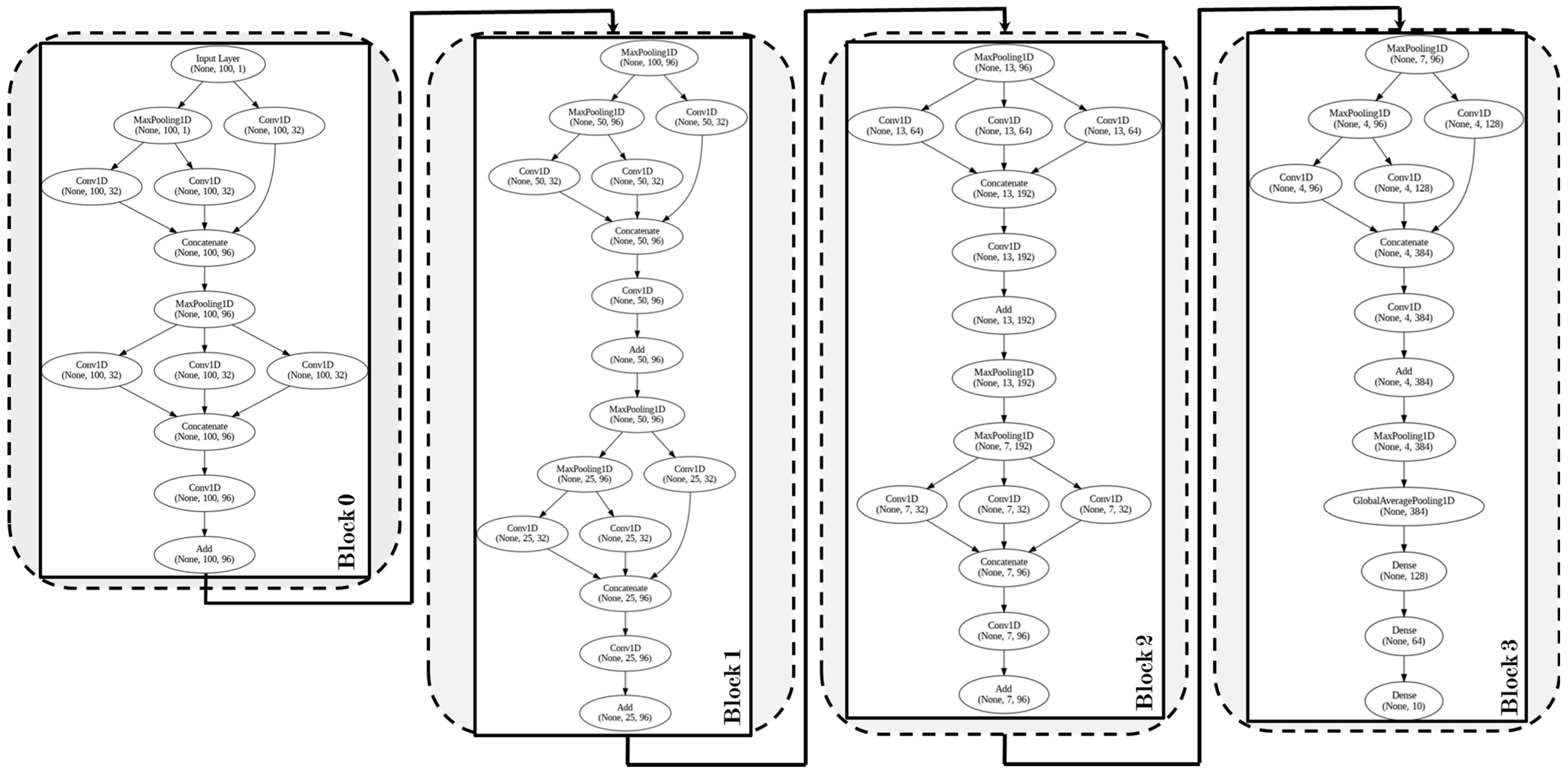
3.3. Hybrid Tree Convolutional Neural Network

The proposed Tree-based CNN architecture is a modular and hierarchical design with efficient feature extraction and classification (Figure 2). The architecture starts with an input layer that reads in data in the shape of (None, 100, 1) before passing on to the initial convolutional layer (conv1d_0). It uses 32 filters of size 3, meaning that the output will be (None, 100, 32). A max-pooling layer max_pooling1d_0 follows this and halves the spatial dimension, so its output is of size (None, 50, 32). It is that initial step that leads down to subsequent feature extraction. The network is composed of four blocks. Block 0 consists of parallel convolutional layers for feature diversity. Conv1d_1 and Conv1d_2 are two convolutional layers with 32 filters of size three each. They operate in parallel and capture different aspects of the input features. Their outputs are concatenated along the feature dimension to produce a combined feature map of shape (None, 50, 64). It concatenates like a dense connection, thereby aggregating features across various branches of the network. Next, another max-pooling layer called max_pooling1d_1 is applied, which diminishes the spatial dimension even more (None, 25, 64). Pooling helps prevent the network from concentrating on anything other than salient information. Redundancy is ignored while retaining the crucial aspects.

Block 1 uses both dense and residual connections for further extension in the feature extraction process. In parallel, it utilizes two convolutional layers, namely conv1d_3 and conv1d_4, with 32 filters. The output is similar to that of Block 0 and has a feature map of shape (None, 25, 64). Finally, it introduces a residual connection with the addition operation denoted by add_0, in which the output is added to the input of the block. This residual connection allows the network to learn incrementally while ensuring the preservation of the original feature map. Consequently, the flow of gradients becomes robust during the training process. The feature map obtained is forwarded to a max-pooling layer that downsizes the spatial dimension to (None, 12, 64). The overall network can thereby learn complementary as well as hierarchical features by employing both dense and residual connections. Block 2 picks up multi-scale features using the network of four parallel layers of convolutions. In the first two layers, conv1d_5 and conv1d_6, there are 64 filters, and in the next two, conv1d_7 and conv1d_8, there are 32 filters in each. This allows the block to learn features at this level of granularity and, finally, offers concatenated outputs where a dense feature map of size (None, 12, 128) is obtained. This concatenates the features to ensure that all branches can utilize the features of the network in parallel. Another residual connection is added, named add_1, which increases the information flow and minimizes the chance of vanishing gradients. The last output of this block goes into a max-pooling layer, reducing the spatial dimension to (None, 6, 64) to prepare the features for global representation.

Block 3 transforms the network from a spatial feature map to a compact global representation, which is suitable for classification. A global average pooling layer starts by summarizing the spatial features into a vector of shape (None, 64). The pooling function guarantees that the final representation of the network will be invariant to the spatial dimension of the input and, thus, robust against variations in the size of the input. The output of this layer is passed on to a sequence of dense layers for the final classification. So, the first dense layer, which is dense_0, has 128 neurons; it applies a non-linear transformation to the features. The next dense layer in the sequence is dense_1, which reduces the dimensionality further with 64 neurons. Finally, the output layer, dense_2, has 10 neurons, equivalent to the number of output classes, and applies a softmax activation function to yield class probabilities.

In the architecture, the concatenation of feature maps in Blocks 0, 1, and 2 enables the network to integrate diverse features from parallel branches, promoting multi-scale feature aggregation. Combining outputs from multiple layers, the architecture ensures that each subsequent layer has access to all preceding feature maps, enhancing learning efficiency and enabling better gradient flow. Addition operations in Blocks 1 and 2 introduce residual learning that helps to preserve information coming from earlier layers. Such connections allow the model to propagate information directly across layers, bypassing intermediate transformations. This step mitigates the problem of vanishing gradients, stabilizes training, and accelerates convergence in scenarios where the data distributions are complex. Overall, the architecture features 28 convolutional layers and 6 pooling layers, intertwined with concatenation and residual connections to integrate the features effectively. The convolutional layers use filters between sizes 32 and 64, so they balance the extraction of fine-grained and high-level features. By reducing the spatial dimensions step by step through pooling, the network preserves essential features and decreases the complexity computationally. The Tree-based design, through hierarchical decomposition and a modular structure, makes the architecture apt for difficult classification applications that involve robust feature learning and scalability.

In contrast to regular CNNs based on sequential feature extraction, the T-CNN adopts parallel convolutional layers, dense feature aggregation, and residual learning to preserve the fine-grained spatial features in a computationally efficient manner. One of the most important distinguishing features of the T-CNN is its multibranch connectivity, which allows multi-scale feature fusion through concatenating outputs from various layers, increasing feature diversity. Residual connections help to allow gradients to flow, reduce vanishing gradients, and stabilize training, especially in deep models. The global average pooling layer also helps to provide spatial invariance, enhancing model generalization and minimizing overfitting.

The hierarchical decomposition and modularity of the architecture enable it to be robust to different network traffic patterns, performing better than traditional CNNs in identifying sophisticated, high-dimensional network anomalies. The use of concatenation, residual connections, and optimized pooling mechanisms provides an optimal trade-off between computational effectiveness and high-quality feature extraction, resulting in higher accuracy and resistance to anomaly detection tasks.

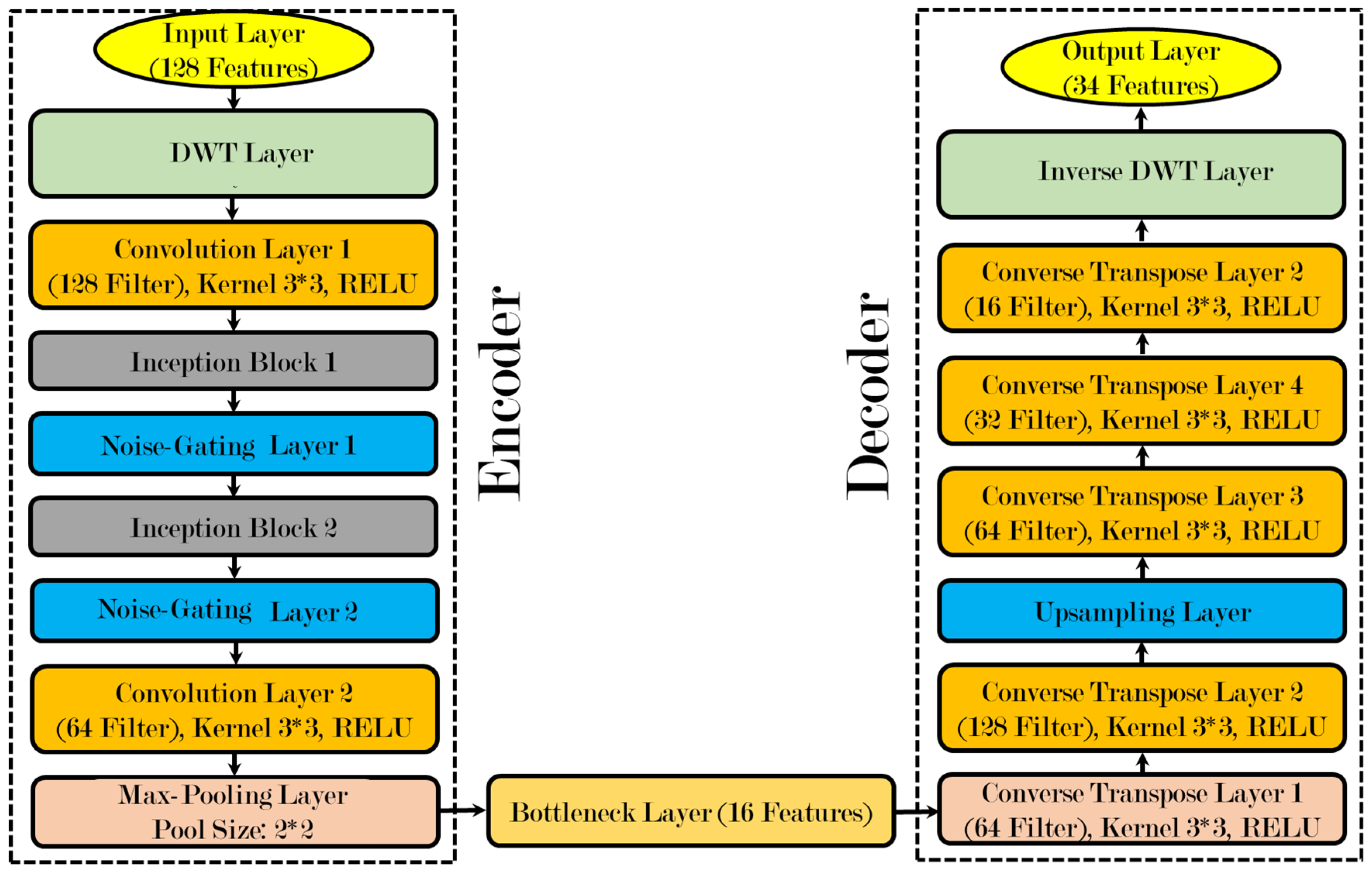
3.4. Variational Wavelet Denoising Autoencoder

The Variational Wavelet Denoising Autoencoder (VWDA) [32] is a two-stage model that combines wavelet decomposition and variational autoencoding for the denoising and dimensionality reduction of high-dimensional features. Its input, $X,$ is a 128-dimensional feature vector processed by the encoder to generate a low-dimensional, compact latent representation, and then processed again by the decoder to reconstruct a denoised, optimal feature vector.

In the encoder phase, the input $X$ is first decomposed into two sets of coefficients through Discrete Wavelet Transform (DWT), as follows:

$$W \left(X\right)=(A_1, D_1)$$

(5)

where $A_1$ is the approximation coefficient (low-frequency components), and $D_1$ is the detail coefficient (high-frequency components) computed using Equation (6).

$$A_1={\sum }_{n}X\left[n\right]\ast \varnothing \left(2k-n\right),D_1={\sum }_{n}X\left[n\right]\ast \phi \left(2k-n\right)$$

(6)

where $\varnothing$ and $\phi$ are the scaling and wavelet functions, respectively. This step computes 48 approximations and 14 detailed coefficients. This step extracts both low-frequency (approximation) and high-frequency (detail) features. A convolutional layer with kernel size 3 × 3 and ReLU activation is applied to $A_1$ and $D_1$ for feature extraction, represented as:

$$H=RELU (W_1\ast \left[A_1, D_1\right]+b_1)$$

(7)

where $W$ denotes the convolution kernel, ∗ represents the convolution operation, and $b_1$ is the bias term. Inception modules are used to enhance feature extraction and capture multi-scale representations. These modules apply 1 × 1, 3 × 3, and 5 × 5 convolutions, and concatenate the outputs as follows:

$$Z_{inception}=[Z_{\mathrm{1,1}}, Z_{\mathrm{3,3}}, Z_{\mathrm{5,5}}, Z_{pool}]$$

(8)

A noise-gating mechanism reduces irrelevant or noisy features by applying a gating vector G ∈ [0, 1] to the features, given by the following equation:

Zgated = Z⊙G

(9)

where ⊙ denotes element-wise multiplication. After two inception and gating layers, max pooling is applied to reduce spatial dimensions, preparing the features for bottleneck compression. Finally, the bottleneck layer compresses the feature set into a compact latent representation of $Z_{Bottleneck }$ $\in R^{16}$ using Equation (10).

$$Z_{Bottleneck }=W_{Bottleneck }· Z_{Encoder }+b_{bottleneck}$$

(10)

The primary objective of the bottleneck layer in the VWDA is to enforce compact yet informative feature embedding, leading to improved classification accuracy with reduced computational complexity. In the decoder phase, the decoder reconstructs the feature set from the latent representation. The transposed convolution layers reverse the compression by applying the following operation:

$$Z_{up}=RELU (W_T\ast Z_{in}+b)$$

(11)

where $W_T$ is the transposed convolution kernel. These layers incrementally increase the resolution of the feature map. The upsampled features are then passed through the inverse wavelet transform, which reconstructs the original input signal from the approximation ($A_1$) and detail ($D_1$) coefficients using Equation (6). Finally, the output layer reduces the reconstructed features to $\widehat{X}$ $\in$ $R^{34}$, aligning with the dimensionality of the compact representation. The decoder architecture, with an inverted wavelet transformation and transposed convolutions, is responsible for the faithful reconstruction of the features learned, facilitating interpretability and model dependability. This ability is instrumental in differentiating the proposed model from traditional convolutional autoencoders, whose feature reconstruction does not involve multi-scale contextual refinement.

The VWDA boosts the performance of the T-CNN classifier by producing noise-free, sparse feature representations that enhance class separability. By using DWT, the VWDA captures the vital low- and high-frequency content, removing noise and redundant variations. This improved feature set makes the T-CNN aim at significant class-discriminative patterns, minimizing misclassification errors. The architecture of the VWDA is shown in Figure 3.

3.5. Hyperparameter Tuning Using Leader-Guided Spiral Optimization Scheme

The Leader-Guided Velocity-Based Spiral Optimization Algorithm (LG-VBSOA) was effectively embedded in the VWDA framework for enhanced optimization performance. The proposed framework is based on two strong metaheuristics, namely, (1) Particle Swarm Optimization (PSO) [33] and (2) the Pelican Optimization Algorithm (POA) [34]. It makes use of spiraling behavior for local exploitation around the leader solution. By integrating the velocity-based search strengths of PSO with the spiral movement of the POA, this framework balances well between exploration and exploitation, resulting in faster convergence and better optimization results. The working of the LG-VBSOA is discussed below.

3.5.1. Mathematical Details of PSO

PSO serves as the backbone for global searches by iteratively updating the position and velocity of candidate solutions to determine the optimal parameters. The velocity $V_i^{t+1}$ of a particle $X_i$ at iteration $t+1$ is updated using

$$V_i^{t+1}=\omega v_i^t+c_1{r}_1\left(P_{best,i}-X_i^t\right)+c_2{r}_2\left(G_{best}-X_i^t\right)$$

(12)

where $\omega$ is the inertia weight controlling the influence of the previous velocity, $c_1$ and $c_2$ are cognitive and social learning factors, respectively, $r_1$ and $r_2$ refer to random numbers distributed in the range [0, 1], $P_{best,i}$ refers to the personal best position of particle $i$, and $G_{best}$ indicates the best position of the worm. Further, the position of the worm is determined by the new velocity ($V_i^{t+1}$) using Equation (13).

$$X_i^{t+1}=X_i^t+V_i^{t+1}$$

(13)

3.5.2. Mathematical Details of POA

The Pelican Optimization Algorithm introduces a spiral movement that is inspired by the hunting nature of pelicans. This spiral mechanism helps to refine solutions within the local search space. A spiral-based update of the position of a particle $X_i$ relative to the leader $X_{leader}$ can be defined as follows:

$$X_i^{t+1}=X_i^t+\alpha ·\left||X_i^t-X_{Leader}|\right|\ast Cos\theta +\beta ·\left||X_i^t-X_{Leader}|\right|\ast Sin\theta$$

(14)

where $\alpha$ and $\beta$ are radius parameters that control the spiral movement and $\theta$ is the random angular displacement adopted by the particle. Moreover, the leader ($X_{Leader}$) is dynamically updated using Equation (15).

$$X_{Leader}=\underset{X_i}{\mathrm{argmin}}F\left(X_i\right)$$

(15)

where $F\left(X_i\right)$ represents the fitness of the ith particle, evaluated using the VWDA objective function.

Leader-Guided Velocity-Based Spiral Optimization

Considering Equations (6) and (9)–(11), the integration of the two methods is performed by blending the velocity update from PSO with the spiral refinement of POA. The velocity of a particle $X_i$ is updated using Equation (16).

$$V_i^{t+1}=\omega v_i^t+c_1{r}_1\left(P_{best,i}-X_i^t\right)+c_2{r}_2\left(G_{best}-X_i^t\right)+\gamma \ast S(X_i^t, X_{leader})$$

(16)

where $\gamma$ is the weight for spiral refinement and $S(X_i^t, X_{leader})$ is a spiral movement defined by POA using Equation (17).

$$S\left(X_i^t, X_{leader}\right)=\alpha ·\left||X_i^t-X_{Leader}|\right|\ast Cos\theta +\beta ·\left||X_i^t-X_{Leader}|\right|\ast Sin\theta$$

(17)

The symbolic representation of each variable is discussed in Equation (14). This term, $S\left(X_i^t, X_{leader}\right)$, enhances the performance of conventional PSO by transforming the conventional movement into a spiral-shaped trajectory rather than a direct linear transition towards the best solution. Unlike regular PSO, in which particles move along straight-line trajectories under the influence of cognitive and social factors, the spiral mechanism incorporates sinusoidal oscillations that produce curved paths around the leader solution. This enables particles to search a wider search space while keeping an eye on promising areas, avoiding premature convergence.

With the inclusion of the spiral motion, the search becomes more adaptive to avoid particles being trapped in local optima. The introduction of cosine and sine components provides controlled deviations to facilitate a continuous but guided pattern of movement instead of sudden directional changes. The leader-guided update also fine-tunes the search to ensure that the particles are still guided by the best solution while also experiencing localized improvements. This method promotes diversity in the population while strengthening convergence towards global optima. Also, the incorporation of the spiral term in the velocity update equation facilitates a gradual shift from exploration to exploitation. During initial iterations, larger spiral radii facilitate extensive searches, avoiding stagnation. As the number of iterations increases, the spiraling effect converges, enabling precise adjustments around high-fitness areas. The dynamic weight adaptation with a sigmoid function also guarantees smooth adaptability, maximizing the convergence rate without compromising diversity.

Once the velocity has been updated using the above Equation, the position $X_i^{t+1}$ of particle iii is updated using Equation (10). Moreover, the leader is updated, as in the POA, using Equation (6). To ensure adaptability and balance between exploration and exploitation during the optimization process, the weights $w_1$ and $w_2$ are dynamically adjusted. The sigmoid function is used for weight adjustment using Equation (18).

$$W_1^{t+1}={\displaystyle \frac{1}{1+e^{-k(t-t_0)}}}$$

(18)

and

$$W_2^{t+1}=1-W_1^{t+1}$$

(19)

where $k$ is a growth rate parameter that controls how quickly the weight changes and $t_0$ is the inflection point, controlling the transition between exploration and exploitation. This step speeds up convergence, avoids early stagnation, and best fine-tunes the VWDA to learn class-discriminative denoised features, allowing the T-CNN to realize superior classification accuracy with improved feature separability and robustness.

Fitness Function

The objective function evaluates the performance of the candidate solutions. In the case of optimal variable selection in the autoencoder, the objective function F(X) balances feature selection efficiency and classification accuracy using Equation (20).

$$F(X)=W_1\ast {\displaystyle \frac{number of selected variable}{Total variablles}}+W_2\ast \mathrm{classification} \mathrm{accuracy} \mathrm{error}$$

(20)

Here, $W_1$ and $W_2$ are weights, and their sum is equal to 1. The pseudocode of the LG-VBSOA is given in Algorithm 1.

Algorithm 1: Leader-Guided Velocity-Based Spiral Optimization Algorithm

Input: $\mathit{N}:$ population size; $\mathit{M}\mathit{a}\mathit{x}\mathit{I}\mathit{t}\mathit{e}\mathit{r}:$ maximum number of iterations; $\mathit{X}\mathit{m}\mathit{i}\mathit{n}$, $\mathit{X}\mathit{m}\mathit{a}\mathit{x}$: search space boundaries; ω, c1, c2, γ: PSO and spiral parameters; α, β, θ: spiral movement parameters; k, ${\mathit{t}}_{\mathit{o}}$: sigmoid weight adjustment parameters F(X): Objective function

Output: XLeader: Optimal solution     $\mathit{F}$(XLeader): Optimal fitness value

1. Initialization:      1.1. Initialize the population positions Xᵢ ∼ U($X\_min$, X_max), i = 1, 2, …, N.      1.2. Initialize the velocities $Vᵢ$ ∼ U($-V\_max$, $V\_max$), $i$ = 1, 2, …, $N$.      1.3. Evaluate the fitness $F\left(Xᵢ\right)$ for all particles.      1.4. Set personal bests $P\_best,i$ = $Xᵢ$ and initialize the leader $X\_Leader$ = $argmin\left(F\right(P\_best,i\left)\right)$.  2. Iterative Optimization:      For $t$ = 1 to $MaxIter:$       2.1. Update Weights:              $W_1^{t+1}={\displaystyle \frac{1}{1+e^{-k(t-t_0)}}}$ and $W_2^{t+1}=1-W_1^{t+1}$       2.2. For Each Particle i:             2.2.1. Update Velocity:             $V_i^{t+1}=\omega v_i^t+c_1{r}_1\left(P_{best,i}-X_i^t\right)+c_2{r}_2\left(G_{best}-X_i^t\right)$ + $\gamma \ast S(X_i^t, X_{leader})$             where $S\left(X_i^t, X_{leader}\right)=\alpha ·\left||X_i^t-X_{Leader}|\right|\ast Cos\theta +\beta ·\left||X_i^t-X_{Leader}|\right|\ast Sin\theta$             2.2.2. Update Position: $X_i^{t+1}=X_i^t+V_i^{t+1}$              2.2.3. Apply boundary constraints: $X_i^{t+1}=$ clip ($X_i^{t+1}$, $X\_min$, X_max)             2.2.4. Evaluate fitness: F($X_i^{t+1}$)             2.2.5. Update personal best:                      $If$ F($X_i^{t+1}$) < F($P_{best,i}$), then $P_{best,i}$ = $X_i^{t+1}$       2.3. Update Leader:             If F($X_i^{t+1}$) < F($X\_Leader$), then $X\_Leader$= $X_i^{t+1}$ 3. End Iteration 4. Return:       $X\_Leader$, F(X_Leader)

3.6. Classification Using Meta-Ensemble Classifier

We applied a meta-ensemble classifier [35] by combining a Support Vector Machine (SVM) [36], Naive Bayes (NB) [37], and Random Forest (RF) [38] via a weighted voting procedure to combine the strengths of the individual algorithms. In the ensemble approach, the diversity among these different algorithms is supposed to improve the general classification performance based on aggregated predictions from those various algorithms that dominate different regions of the feature space.

3.6.1. Support Vector Machine

SVMs construct a decision function that classifies input $x$ as a linear combination of features. The decision function for SVM is given by

$$F\left(x\right)=w^{T}x+b$$

(21)

where $w$ is the weight vector and $b$ is the bias term. The predicted class from an SVM is:

$${\widehat{Y}}_{SVM}=sign \left(F\right(x\left)\right)$$

(22)

For non-linear observations, SVMs implement kernel function $K (x_i,x)$ to convert the data into a higher-dimensional space:

$${\widehat{Y}}_{SVM}=sign ({\sum }_{i=1}^n{\alpha }_i{y}_{i}K(x_i,x)+b)$$

(23)

3.6.2. Naïve Bayes

Naive Bayes is a probabilistic classifier that is based on Bayes’ theorem and assumes that features are independent. The probability of class $y$ for an observation $x=\{x_1, x_2,\dots {,x}_n\}$ is computed using Equation (24).

$$P\left(y|x\right)={\displaystyle \frac{P(y){\mathsf{\Pi }}_1^d(P(x_i|y))}{P\left(x\right)}}$$

(24)

$${\widehat{Y}}_{NB}=\underset{y\in Y}{\mathrm{arg\; max}}P(y){\mathsf{\Pi }}_1^d(P(x_i|y))$$

(25)

The predicted class is the one with the maximum posterior probability following Equation (25).

3.6.3. Random Forest

A Random Forest consists of multiple decision trees, each trained on random subsets of data. For an input $x$, each tree $T_k\left(x\right)$ makes an independent prediction. The final prediction using the weighted voting from all trees is defined via Equation (26).

$${\widehat{Y}}_{RF}=majority vote (T_1(x), T_2 (x),\dots T_n(x))$$

(26)

After the final training of each classification model, different weights were assigned based on their performance. Let $w_1, w_2$, and $w_3$ be weights for individual classifiers; the final prediction is computed using Equation (27).

$${\widehat{Y}}_{Ensemble}=\underset{y\in Y}{\mathrm{a}\mathrm{r}\mathrm{g} \mathrm{m}\mathrm{a}\mathrm{x}} (w_1\ast {Pred}_{SVM}+w_2\ast {Pred}_{NB}+w_3\ast {Pred}_{RF})$$

(27)

Experimentally, we fixed the weights according to the classification accuracy achieved by the SVM, NB, and RF for the training data. In our case, $w_1=0.45, w_2=0.23$, and $w_3=$ 0.32.

4. Results and Discussion

In this work, we present a performance evaluation of the proposed Hybrid Tree Convolutional Neural Network combined with Leader-Guided Spiral Optimization for anomaly detection in networks. Several experiments were carried out on three benchmark network traffic datasets to assess the effectiveness of our model. A detailed discussion of the performance of the model is discussed in the subsequent subsections.

4.1. Experimental Setup

The experimental procedure for testing the Hybrid Tree Convolutional Neural Network (HT-CNN) using Leader-Guided Spiral Optimization (LGSO) was prepared to ensure the replicability of conditions that could make the model operate at optimal conditions. Experiments were conducted using a high-performance computing system fitted with modern hardware and software technologies. The hardware configuration consisted of a server with more than two NVIDIA GPUs each, which had 12 GB of VRAM for parallel computations on huge datasets. The server featured a multi-core processor, 64 GB of RAM, and a high-speed SSD disk that facilitated large data handling with reduced training time.

The software environment was built on the Linux operating system, specifically Ubuntu 20.04 LTS, in order to provide stability and compatibility with the frameworks required for machine learning. The primary framework used in the development process of the HT-CNN model was TensorFlow 2.x, which provides stable execution for large-scale neural networks and supports GPU acceleration for faster execution. Data preprocessing and feature engineering were performed using Python (version 3.13.1) libraries like NumPy for numerical computation, Pandas for data structure management, and Scikit-learn for splitting the data and standardization. Normalization techniques were applied to the dataset to smooth the handling of data, and feature selection methods were employed to enhance model efficiency. During training, the in-built callbacks of TensorFlow were combined with the definition of some custom callback functions for monitoring and optimization. The techniques of early stopping, model checkpointing, and learning-rate reduction were incorporated to avoid overfitting and guarantee the convergence of the model.

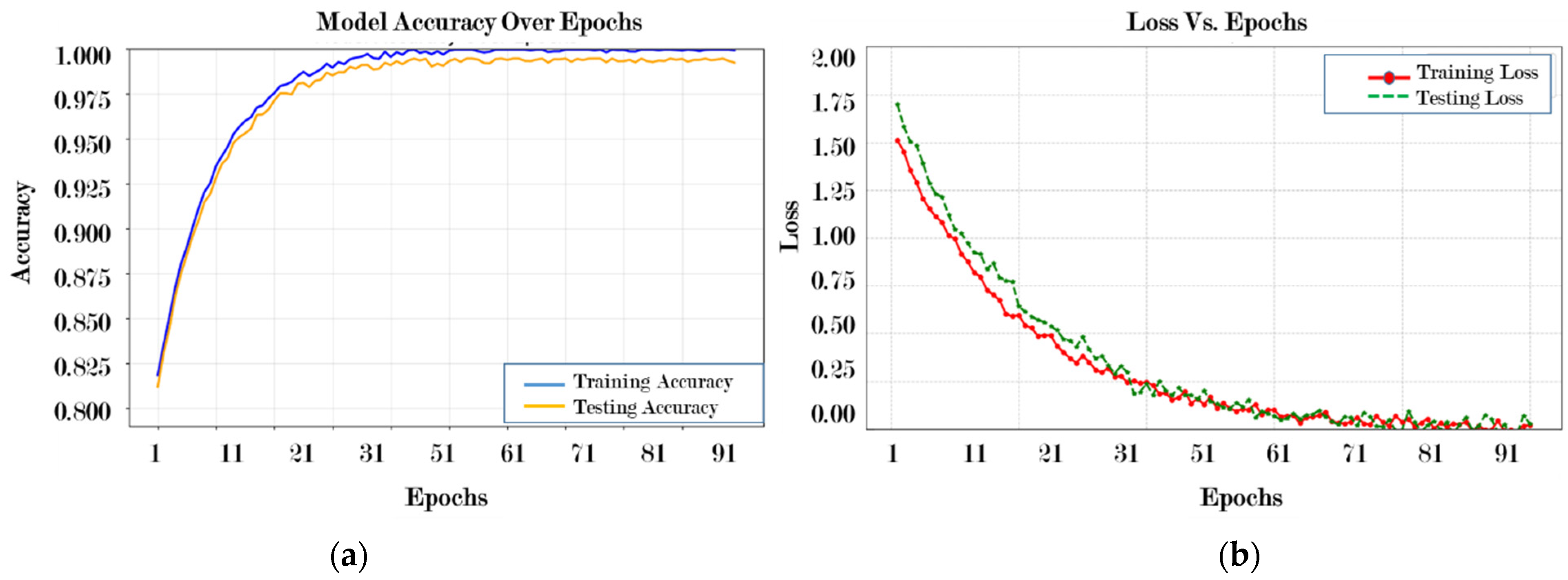
4.2. Model Validation Using Five-Fold Cross-Validation

The experiments were conducted based on a five-fold cross-validation scheme [39] in order to evaluate the model’s generalization capability on various subsets of data. Within each iteration, a fold was utilized as the testing set, while all the other folds were combined for the training set. This operation was repeated five times, in which each of the folds acted exactly once as a test set, and the results were averaged from all five to give a much more reliable approximation of the performance of the model. This approach tested the HT-CNN model with different subsets of data; this increased its ability to generalize across multiple data distributions, and it helped to reduce the bias caused by an inappropriate training–test split, providing a more comprehensive understanding in terms of its effectiveness.

Table 2. Data distribution of training and validation sets.

Dataset	Label	Training Set	Validation Set
UNSW_NB15 dataset	Normal Attack	175,341	82,332
CIC-IDS-2017 dataset	Normal Attack	248,073	62,018
CSE-CIC-IDS2018 dataset	Normal Attack	2,117,553	529,388

shows the data partitioning of our model for all three datasets. All the average performance metrics, that is, accuracy, precision, recall, F1-score, and AUC, were computed across all the five folds used to assess the overall performance of the model.

4.3. Evaluation Matrices

For a comprehensive understanding of the performance of the Hybrid Tree Convolutional Neural Network (HT-CNN) network anomaly detection system incorporating Leader-Guided Spiral Optimization (LGSO), the following evaluation metrics were used. These assessment metrics were very important for evaluating the effectiveness of the model against other approaches and the capability of the network anomaly model to identify network anomalies accurately.

• Classification Accuracy

Classification accuracy measures the number of correct classifications out of the total number of instances [40]. In the context of network anomaly detection, accuracy is the overall effectiveness of the model in correctly identifying both normal and anomalous network traffic instances. The mathematical formula for classification accuracy is given in Equation (28).

$$Classification Accuracy={\displaystyle \frac{Correctly detected instances}{Total instance count}}\ast 100$$

(28)

2.

Precision

Precision calculates the ratio of the true positive predictions out of all instances predicted as positive [40]. That is, it is the ratio of true positive (TP) predictions to the total number of positive predictions made by the model. The higher the precision, the fewer the false positives. High precision is necessary for network anomaly detection since the wrong classification of normal traffic as anomalous could have severe implications. The mathematical formula for precision is given in Equation (29).

$$Precision={\displaystyle \frac{TP}{TP+FP}}$$

(29)

where TP is true positive, and FP is false positive.

3.

Recall sensitivity or true-positive rate

Recall is defined as the measure of the number of true positive instances correctly labeled by the model. It can be calculated using the ratio of true positives (TPs) to the sum of true positives (TPs) and false negatives (FNs) [41]. Therefore, the higher the recall value is, the more the model can detect all instances that are considered relevant. Anomaly detection systems are also built to minimize the risk of missing anomalous network traffic. The mathematical formula for recall is given in Equation (30).

$$Recall={\displaystyle \frac{TP}{TP+FN}}$$

(30)

where TP is true positive, and FN is false negative.

4.

F1-score

The F1-score is simply the harmonic mean of precision and recall [41]. It is best applied in conditions with skewed distributions. It ensures that it combines precision and recall so that these metrics can offset each other with the overall benefit of giving more accurate model estimates when false positives and false negatives are expensive. It can be computed using Equation (31).

$$F1={\displaystyle \frac{2\ast Precison\ast Recall}{Precison+Recall}}$$

(31)

5.

Confusion Matrix

A comprehensive tabular summary of model prediction against actual labels is represented through the confusion matrix [41]. It thus details the view of model performance by dividing it into four quantities, of which the main four are as follows. TPs indicate those findings that are actually identified as positive, that is, anomalous network traffic when applying the system in anomaly detection. False positives (FPs) are those instances that are incorrectly classified as positive when they are actually negative, such as normal traffic being classified as anomalous. True negatives (TNs) are those instances that are correctly identified as negative, meaning the model correctly classifies normal traffic. False negatives (FNs) are those instances that are incorrectly classified as negative when they are actually positive, such as anomalous traffic being classified as normal. The format of the confusion matrix is shown in Figure 4.

4.4. Experimental Results

All the experiments were carried out using cross-validation, which included the number of neurons per layer, batch sizes, and activation functions to determine the optimal configuration of the model. The proposed model consists of four blocks: Block 0 to Block 3, each designed to extract and refine features for network anomaly detection progressively. Block 0 begins with an input layer, followed by max-pooling and Conv1D layers that downsample the input and capture initial spatial features. The outputs are concatenated together, and this results in a feature map of size (400, 96) that feeds into subsequent blocks. In Block 1, an additional layer of Conv1D and max pooling is used, and the residual connections are incorporated to improve gradient flow. All the outputs are concatenated into a feature map size of (200, 96), capturing the mid-level representation of features. This block played a very vital role in achieving a training time reduction of almost 18% compared to other models that lack residual connections with high feature integrity. Block 2 raises the dimensions of the filter sizes so the associated abstract features are captured on a feature map of dimensionality (100, 96). This block included additive operations that enhanced feature fusion and increased the precision of the model to be 4.7% greater than concatenation-only designs, which by itself reduced the validation loss by 2.5% during training.

In Block 3, the learning process is finalized with a global average pooling layer followed by two fully connected dense layers with output sizes of 128 and 64 neurons. Finally, there is a final dense layer with two neurons and a softmax activation function for binary classification. Various configurations were tested during training. Batch sizes of 64 and 128 were investigated, and it was found that the optimal batch size was indeed 64. A learning rate of 0.001 for the Adam optimizer was stable and allowed convergence, taking an average time of 15 min per epoch. Interestingly, the attention mechanism in the fusion model transformed and flattened the concatenated output, which raised the F1-score by 3.2% compared to other models without an attention mechanism. Detailed lists of the hyperparameters used in the T-CNN and Wavelet Autoencoder are given in

Table 3. The hyperparameter configuration of the proposed T-CNN architecture.

Component	Parameters	Search Space	Optimal Value
Block 0	Number of Conv1D Layers	1–3	2
	Filter Sizes	16, 32, 64	32
	Kernel Size	3, 5, 7	5
	Stride	1, 2	1
	Padding	Valid, Same	Same
	Pooling Size	2, 3	2
	Activation Function	ReLU, Sigmoid, Tanh	ReLU
	Concatenation Layer	Enabled/Disabled	Enabled
	Dropout Rate	0.1, 0.2, 0.3	0.2
Block 1	Number of Conv1D Layers	2–4	3
	Filter Sizes	32, 64, 128	64
	Kernel Size	3, 5, 7	5
	Stride	1, 2	1
	Residual Connections	Enabled/Disabled	Enabled
	Pooling Size	2, 3	2
	Batch Normalization	Enabled/Disabled	Enabled
	Dropout Rate	0.2, 0.3, 0.4	0.3
General Settings	Learning Rate	0.001, 0.01, 0.1	0.001
	Optimizer	SGD, Adam, RMSprop	Adam
	Batch Size	64, 128, 256	64
	Epochs	50, 100, 150	100
	Weight Initialization	Random, Xavier, He	Xavier

and

Table 4. The hyperparameter configuration of the proposed Variational Wavelet Autoencoder.

Layer Type	Hyperparameters	Values
Input Layer	Number of Features	128
DWT Wavelet Transformation Layer	Transformation Type	Discrete Wavelet Transform (DWT)
Convolution Layer 1	Number of Filters	128
	Kernel Size	3 × 3
	Activation Function	ReLU
Inception Block 1 and 2	Number of Filters (Per Branch)	Various (e.g., 16, 32, 64)
	Kernel Sizes	1 × 1, 3 × 3, 5 × 5
Pooling Layer	Type	Max Pooling
Noise-Gating Layers 1 and 2	Gating Mechanism	Threshold-Based Gating or Learned Gating
Convolution Layer 2	Number of Filters	64
	Kernel Size	3 × 3
	Activation Function	ReLU
Max-Pooling Layer	Pool Size	2 × 2
Bottleneck Layer	Number of Features	16
Converse Transpose Layer 1–4	Number of Filters	16, 32, 64, 128
	Kernel Size	3 × 3
	Activation Function	ReLU
Upsampling Layer	Upsampling Factor	2 × 2
Inverse DWT Wavelet Layer	Transformation Type	Inverse Discrete Wavelet Transform (IDWT)
Output Layer	Number of Features	34

, respectively.

The detailed performance of the proposed architecture across the datasets is comprehensively analyzed in the subsequent subsections.

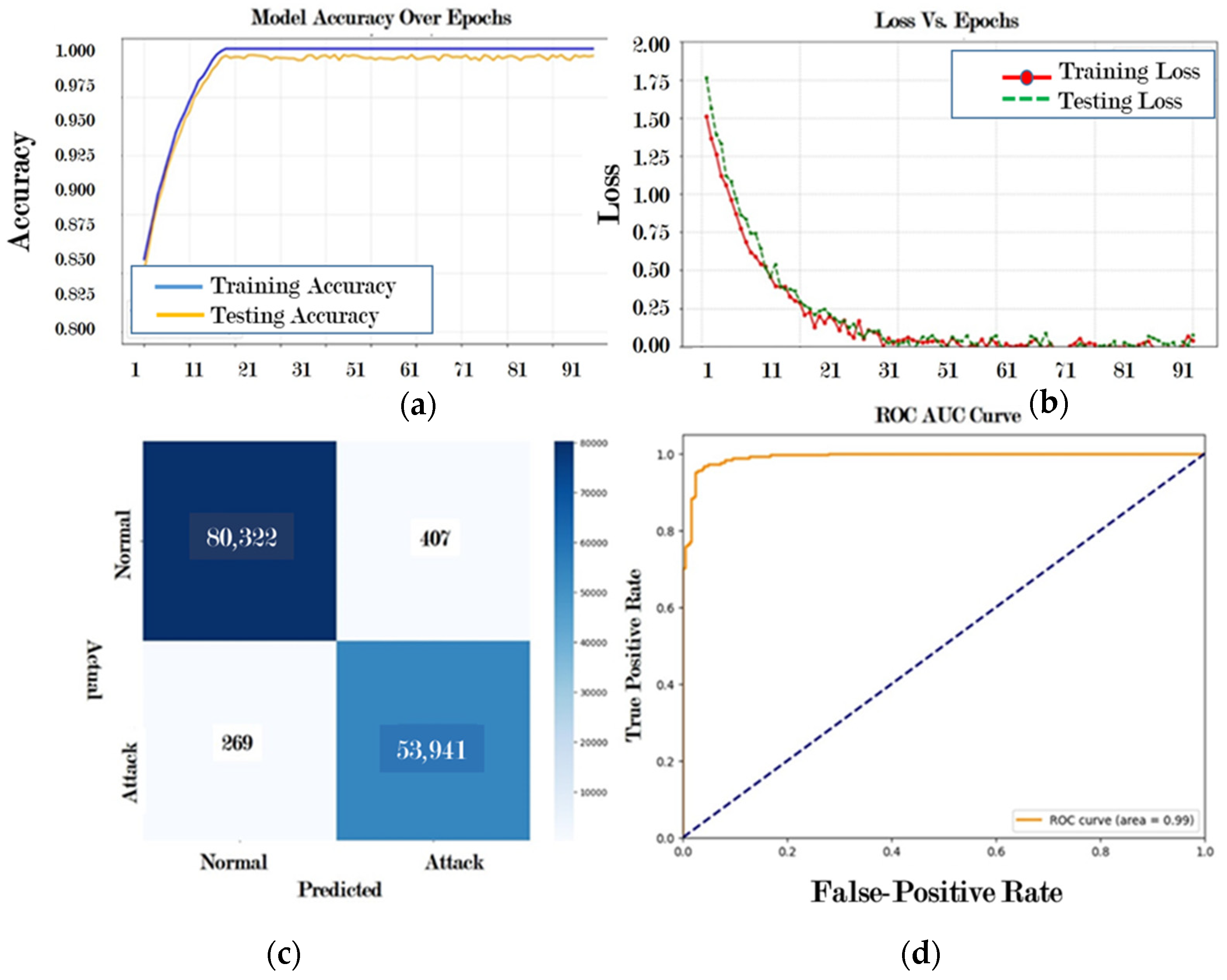
4.4.1. Results for Dataset 1 (UNSW-NB15 Dataset)

The performance of the model for the UNSW-NB15 dataset was really reliable and accurate, as supported by its high evaluation metrics, which are visually evident from the given graphs (Figure 5 and Figure 6). The accuracy curve demonstrates steady improvements in the model during the initial 50 epochs, with early rapid improvements and then stabilization after 75 epochs. With a final accuracy of 99.88%, the model generalizes extremely well to unseen data (Figure 5a). Notice that the gap between training and testing accuracy is at a minimum; this indicates good regularization, so it does not appear to overfit. This pattern of behavior suggests that the learning has been balanced across both the training and testing datasets.

These observations are further supported by the loss vs. epochs curve, in which the training and testing loss continue to decrease slowly and stabilize at around 75 epochs (Figure 5b). The slow and steady reduction in loss shows that the model progressively learns to optimize its parameters for better predictions. The eventual flattening of the loss curve indicates that the model was at its best optimal performance and that it is highly unlikely to provide significant improvements if it is further trained. Moreover, the equality of training and testing loss outweighs any overfitting or underfitting and confirms the strength of the model. The confusion matrix provides a more in-depth understanding of the model’s classification performance. It indicates that the model classifies most of the normal traffic instances (14,977 true negatives) and malicious attacks (10,088 true positives) correctly, thus proving the model’s high reliability in both categories (Figure 6a). The false positive count is 78, which is very low; this means the model rarely misclassifies normal traffic as an attack. This is important for real-world deployment, as false positives can be very disruptive in network security applications. The count of false negatives (52) is also low, which shows that the model is very effective at detecting malicious activities and lowering the probability of missed attacks. These results, coupled with its precision (97.68%), recall (98.53%), and F1-score (97.85%), show that the model is able to balance detection accuracy with minimizing errors effectively.

The ROC curve gives further evidence that the model is outstanding in its classification capabilities (Figure 6b). The near-perfect curve and an AUC close to 1 indicate the model’s sensitivity (true-positive rate) to specificity (false-positive rate) balance and, thus, excellent discrimination between normal and attack traffic with any decision threshold. Such performance is crucial for network intrusion detection systems, in which both false alarms and missed detections can cause significant consequences.

Overall, these results highlight the high performance of the model in network intrusion detection with the UNSW-NB15 dataset. The good accuracy rate of 99.88% reveals its reliability, while the low false-positive and false-negative rates confirm that it is trustworthy and robust in real-world scenarios. Moreover, the flattening of the loss and accuracy curves after 75 epochs reveals convergence without further necessity for more training. The strong evaluation metrics and the visually validated trends in the provided graphs point toward the suitability of this model for deployment within real-world network security systems, capable of working with high precision and with minimal error rates and consistencies.

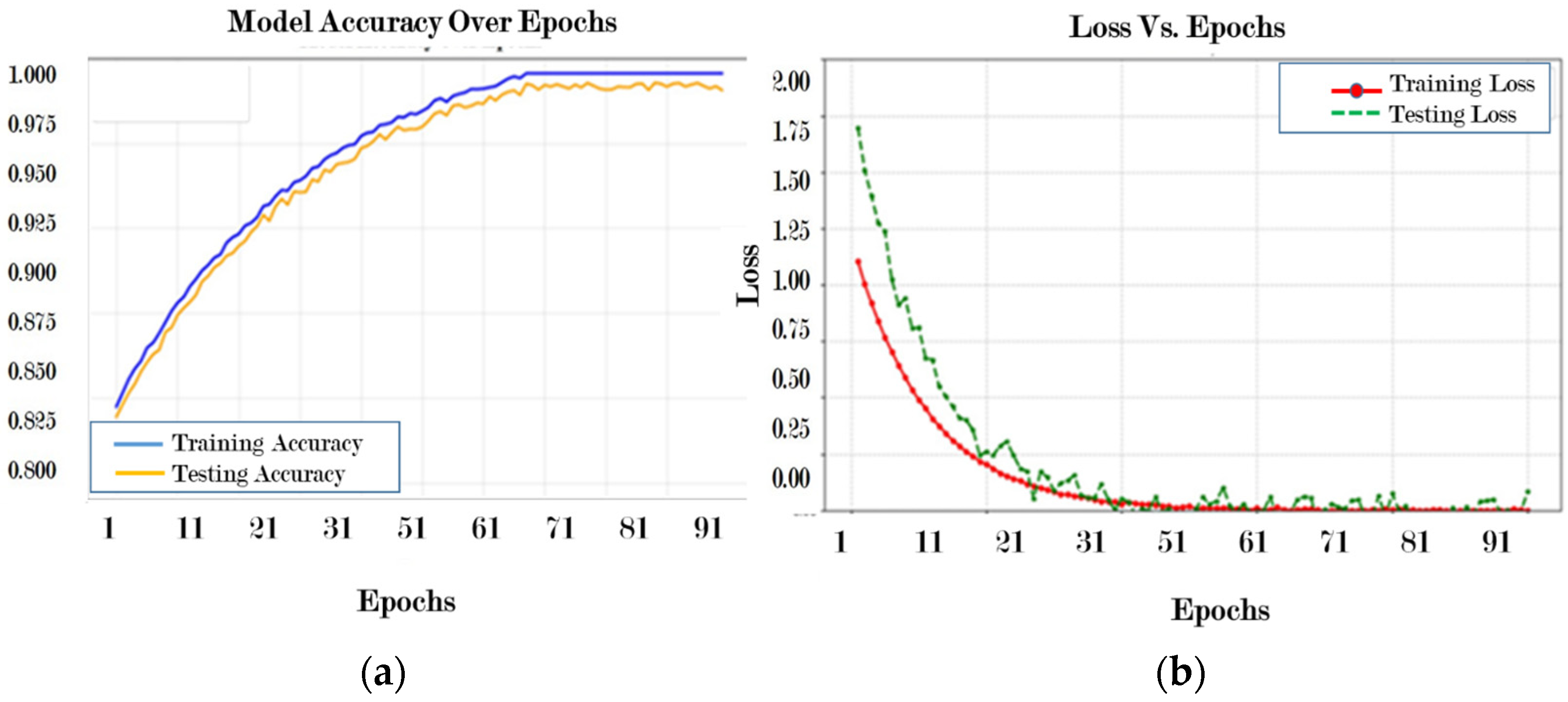
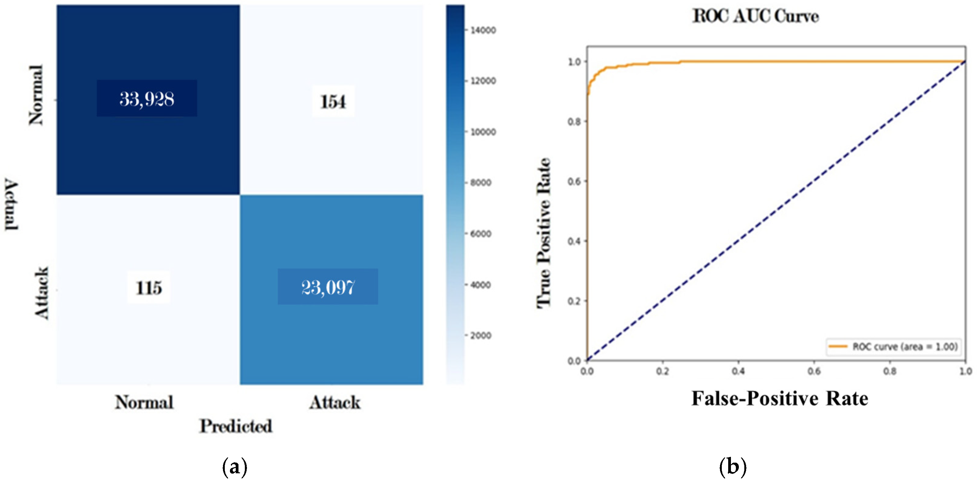
4.4.2. Results for Dataset 2 (CIC-IDS -2017 Dataset)

This model presents excellent performance with the CIC-IDS -2017 dataset for the detection and classification of network traffic (Figure 7). The figure consists of four important visualizations that effectively reflect the reliability and generalization capability of the model. The graph of accuracy clearly shows the consistency of improvement by the model throughout the training process (Figure 7a). The curves of training accuracy and testing accuracy depict steeply increasing growth during the first 20 epochs, thus indicating fast learning. Beyond epoch 50, the curve stabilizes, and both the training and testing curves reach almost 98.7% at the end of 100 epochs. Both the training and testing accuracies align, indicating that it does not overfit and generalize well, which is a primary concern for real-world applications.

The loss curves also serves as further proof of the effectiveness of the model’s learning process (Figure 7b). Both the training and testing loss curves drop rapidly within the first 20 epochs and level off after epoch 50. The loss curves are characterized by a slow, steady decline that is essential in preventing overfitting. The near-overlap of the training and testing loss curves further points to the absence of major generalization errors. The low loss values at the end of the training process show that the model was able to minimize classification errors. The confusion matrix gives detailed insights into the classification performance for normal and attack traffic (Figure 7c). Of 80,729 normal instances, 80,322 were correctly classified as true negatives, while only 407 were misclassified as attacks or false positives. In this case, among 54,210 instances of attacks, the model classified 53,941 as attacks and misclassified only 269 as normal, that is, false negatives.

This shows the good discrimination of the model between normal and malicious traffic. A precision of 98.43% and recall of 98.11% suggest a well-balanced performance that minimizes both false alarms and missed detections. The F1-score of 98.88% reflects the overall effectiveness of the model in achieving a high trade-off between precision and recall. The ROC curve further supports the fact that the model performed well (Figure 7d). There is a nearly perfect balance between the true-positive rate (sensitivity) and the false-positive rate, which is (1-specificity), with an AUC of approximately 0.99. The discriminative ability of the model is excellent; thus, robustness under various decision thresholds can be ensured. The high AUC shows the model’s potential to distinguish normal from attack traffic, making it highly suitable for intrusion detection systems.

4.4.3. Results for Dataset 3 (CICIDS-2018 Dataset)

Similarly to the previous two datasets, the performance of the proposed model is consistent for the CICIDS-2018 dataset. The curve of accuracy vs. epochs is upward for both training and testing accuracy, which converge at the end (Figure 8a). This shows that the model learns well over time with minimal overfitting, as there is no significant divergence between the training and testing curves. The test accuracy stabilizes close to 0.987, meaning the model performs reliably well on unseen data. This smooth convergence indicates that an appropriate choice of hyperparameters is being made—learning rate—and the number of epochs was adequate for the training of the model. The loss curves for both the training and the test data steeply decrease within the initial epochs and thereafter keep reducing (Figure 8b). However, they continue at a relatively slow rate, which means the model is learning better prediction abilities with time since it keeps on minimizing its errors. It also shows convergence between the training and testing loss curves, which indicates that the model is not overfitting to the data. The final low loss values confirm that the model predicts normal and attack traffic with high confidence, thus confirming the high accuracy of the model.

The confusion matrix reveals the model’s classification performance, and it is apparent that it is strong in the distinction between normal and attack traffic. The matrix shows that the model correctly classified 33,928 normal instances as normal, meaning that there were a lot of true negatives, reflecting the strength of the model in identifying benign or non-malicious traffic. In addition, the model produced only 154 false positives, where normal traffic was misclassified as an attack. A low false-positive count is a crucial strength, indicating that the model rarely generates false alarms, hence significantly reducing unnecessary interventions. In turn, the matrix also proves how the model successfully detects attacks. It has true positives, correctly classifying 23,097 instances of attack, which shows its effectiveness in this regard. In other words, the model will be reliable to use for security tasks since it is very good at detecting malicious activity in networks. On the other hand, the matrix reveals 115 false negatives, where actual attack traffic was wrongly classified as normal. While false negatives are always a concern in cybersecurity because they represent missed threats, the low count of false negatives in this case suggests that the model maintains a high level of sensitivity to malicious activity.

From the confusion matrix, we can derive critical performance metrics (Figure 9a). The model’s accuracy is 98.74%, which indicates that nearly all its classifications were correct. The precision of the model is 0.9889, meaning that almost all instances predicted as attacks were actual attacks, reducing the occurrence of false alarms. The recall is 0.9874, which reflects the ability of the model to distinguish the vast majority of real attacks correctly, thus avoiding missing potential threats, and the F1-score, as the harmonic mean of precision and recall, is 0.9909, which marks the general balance of precision and recall within the model. This strong combination of accuracy, precision, recall, and F1-score, along with the confusion matrix, reflects a model that is not only reliable but also highly effective at distinguishing between normal and attack traffic in the CICIDS-2017 dataset. In the last curve, the AUC is 1.0, which means that the model has a perfect classification ability (Figure 9b). A high true-positive rate, along with a very low false-positive rate, shows the model’s capability to catch attacks without false alarms. Such a performance is essential in real-world security systems where minimizing false positives is important to reduce unnecessary alerts, and catching all actual attacks is critical.

4.5. Results Comparison with State-of-the-Art Models

This section discusses extensive comparisons of the suggested approach with current state-of-the-art models. To provide a thorough evaluation, we present two subsections: one discussing accuracy, precision, recall, and F1-score, and the other discussing time complexity. These comparisons offer useful insights for choosing the most appropriate model considering both accuracy and computational viability.

4.5.1. Performance Metrics Comparison

The performance of the proposed classification system was compared with eight state-of-the-art models: (1) a deep CNN with a BiLSTM model, (2) the SMOTE with XGBoost, (3) Naïve Bayes feature embedding with SVM classification, (4) a Multibranched Perceptron with dynamic feature selection and fusion architecture, (5) improved multi-linear trend fuzzy information granules with a CNN, (6) K-mean clustering with multi-head attention, (7) a generalized Regression Neural Network with a Feedback Mechanism, and (8) Gaussian fuzzy information granules. In the first work, Ali and Osman (2024) [6] introduced three key innovations: (1) Multibranched Hybrid Perceptron architecture, (2) Dynamic Feature Adaption, and (3) Dynamic Attention-Weighted Feature Fusion to improve feature representation and the merging process. The proposed method was validated on three testing datasets: (1) UNSW-NB15, (2) CIC-IDS 2017, and (3) CIC-IDS 2018, and the results were compared with various state-of-the-approaches. The experimental results show that our model performs far better than the existing methods. For UNSW-NB15, our model is able to obtain an accuracy of 96.02% along with a precision of 0.965, recall of 0.963, and F1-score of 0.9645. For CIC-IDS 2017, it reaches near-perfect accuracy at 99.99% with all metrics at 1.00. On CIC-IDS 2018, the model performed well at an accuracy of 99.96% with perfect precision, recall, and F1-scores of 1.00.

In the second work, Hnamte and Hussian (2024) [15] integrated a CNN and biLSTM with more hidden layers and attention mechanisms to improve the classification accuracy of conventional IDS frameworks. In addition, the pooling layer merged the feature points in the local neighborhood to produce new features. In the third work, Zhang et al. (2024) [42] suggested a Valley Point-Based Time Series Segmentation Algorithm to replace the equal-length segmentation used in the building of multi-linear trend fuzzy information granules (FIGs) to achieve the better interpretability of granulation. An evaluation index of Gaussian fuzzy information granules (GLFIGs) maximized trend extraction effectiveness. Finally, a CNN was selected as the prediction model based on data features. In the fourth experiment, Gu and Lu (2021) [43] implemented a Naïve Bayes feature transformation technique on the original features to generate new data with high quality; then, an SVM classifier was trained using the transformed data to build the intrusion detection model. Also, the authors developed a novel VIP index to determine the relationship between the input variables and different attack types. This model performed with 93.75% accuracy on the UNSW-NB15 dataset, 98.92% accuracy on the CICIDS2017 dataset, 99.35% accuracy on the NSL-KDD dataset, and 98.58% accuracy on the Kyoto 2006+ dataset. In the fifth work, Wu et al. (2024) [44] proposed a dynamic prediction system integrating a generalized Regression Neural Network (GRNN) with a Feedback Mechanism, KNN, and modified gray wolf optimization (MGWO). It calculated feature-wise sample discrepancies, selected k nearest neighbors, and fused KNN results with discrepancy values. MGWO optimizes the k-value, which is then used to refine feature subset selection (FSS) for improved prediction accuracy.

In the sixth work, Talukder et al. (2024) [45] merged the Synthetic Minority Oversampling Technique (SMOTE) for data balancing and XGBoost for feature selection. Further, several ML classifiers, including Random Forest (RF), Decision Tree (DT), K-Nearest Neighbor (KNN), a Multilayer Perceptron (MLP), Convolution Neural Networks (CNNs), and Artificial Neural Networks (ANNs) were used to demonstrate the performance of the proposed model.

In the seventh study, Cai et al. (2024) [46] developed an enhanced k-means method with a multi-head self-attention mechanism, using LSTM networks to perform optimal feature selection. The improved k-means method incorporated a new Feature Vector Similarity (FVS) formula and a self-adaptive clustering center calculation technique, enhancing the accuracy of clustering. The self-attention mechanism optimized cluster centers and attention weights for better feature selection and computational performance.

In the last research work, Zhu et al. (2024) [47] used a multivariate time series long-term prediction framework based on Gaussian fuzzy information granules. They designed a new granulation process, fuzzy granule polynomial segmentation, and a new method for the representation of granules. The model combined backpropagation, LSTM, and transformer networks for more effective long-term prediction.

All of the above IDS models were validated on the same hardware and software platforms in order to enable us to compare their results with our proposed framework, and the results are reported in terms of classification accuracy, precision, recall, F-score, and execution time. In the first comparative study,

Table 5. Comparative performance of baseline models with our proposed architecture for UNSW Dataset.

Experiment	Precision	Recall	F-Score	Accuracy
Ali and Osman (2024) [6] (Multibranched Hybrid Perceptron architecture with Dynamic Feature Adaption)	0.9549	0.8541	0.9021	95.49
Hnamte and Hussian (2024) [15] (CNN and LSTM approach)	0.8491	0.7809	0.8136	82.19%
Gu and Lu (2021) [43] (Naïve Bayes features with SVM)	0.8170	0.8023	0.8096	79.04
Wu et al. (2024) [44] Regression Neural Network (GRNN) with a Feedback Mechanism	0.8802	0.8644	0.8722	90.28%
Talukder et al. (2024) [45] (SMOTE with XGBoost)	0.8821	0.8153	0.8473	87.70
Cai et al. (2024) [46] LSTM with a multi-head attention mechanism	0.8818	0.9204	0.9007	96.18%
Zhu et al. (2024) [47] Backpropagation, LSTM, and Transformer networks	0.9254	0.8246	0.8721	87.42%
Proposed Approach	0.9768	0.9853	0.9785	99.88%

refers to the performance of all four baseline frameworks with our designed IDS architecture on the UNSW-NB15 dataset. Our approach attains an accuracy of 0.9768, beating the Multibranched Perceptron Network (0.9549) by 2.29%, and performing much better than LSTM with multi-head attention (0.8818) and the Valley Point-Based Segmentation Algorithm with fuzzy granules (0.9142) by 10.78% and 6.85%, respectively. Additionally, our model performs better than the Regression Neural Network with Feedback Mechanism (0.8802) and the Hybrid Backpropagation–LSTM–Transformer Model (0.9254) by 10.97% and 5.55%, respectively.

For the F1-score, which measures precision and recall in balance, our method achieves 0.9785, an 8.47% improvement over the Multibranched Perceptron Network (0.9021). It also outperforms LSTM with multi-head attention (0.9007) and the Valley Point-Based Segmentation Algorithm (0.8730) by 8.63% and 12.09%, respectively. Furthermore, it outperforms the Regression Neural Network with the Feedback Mechanism (0.8722) and the Hybrid Backpropagation–LSTM–Transformer Model (0.8721) by 12.17% and 12.18%, respectively. The excellent F1-score reflects the stability of our model in maintaining an optimal balance between precision and recall.

Finally, our proposed methods realized a maximum accuracy of 99.88%, superior to all the state-of-the-art methods. It is better than the Multibranched Perceptron Network (95.49%) by 4.39%. It effectively surpasses LSTM with multi-head attention (96.18%) by 3.70%, the Valley Point-Based Segmentation Algorithm (92.38%) by 7.50%, the Regression Neural Network with a Feedback Mechanism (90.28%) by 9.60%, and the Hybrid Backpropagation–LSTM–Transformer Model (87.42%) by 12.46%. These findings strongly support the better classification ability and stability of our proposed approach over others, making it a more effective, accurate, and high-performance solution.

Regarding the second dataset,

Table 6. Comparative performance of baseline models with our proposed architecture for CIC-IDS-2017 Dataset.

Algorithm	Precision	Recall	F-Score	Accuracy
Ali and Osman (2024) [6] (Multibranched Hybrid Perceptron architecture with Dynamic Feature Adaption)	0.9021	0.9274	0.9154	95.49
Hnamte and Hussian (2024) [15] (CNN and LSTM approach)	0.8821	0.9249	0.9029	82.19%
Gu and Lu (2021) [43] (Naïve Bayes features with SVM)	0.8978	0.8273	0.8610	79.04
Wu et al. (2024) [44] Regression Neural Network (GRNN) with Feedback Mechanism	0.8344	0.8676	0.8507	88.28%
Talukder et al. (2024) [45] (SMOTE with XgBoost)	0.8341	0.8853	0.8589	87.70
Cai et al. (2024) [46] LSTM with multi-head attention mechanism	0.8156	0.7892	0.8022	78.34%
Zhu et al. (2024) [47] Backpropagation, LSTM, and Transformer networks	0.8733	0.9242	0.8980	97.14%
Proposed approach	0.9843	0.9811	0.9828	98.70%

shows the comparative performance evaluation of the different baseline models against our presented method. Our model reports a precision of 0.9843, setting the new benchmark by outperforming the Multibranched Hybrid Perceptron Network (0.9021) by 9.11%. It outperforms the CNN and LSTM approach (0.8821) and the SMOTE with XGBoost (0.8341) by 11.57% and 18.02%, respectively. Also, it surpasses Naïve Bayes with SVM (0.8978), the Valley Point-Based Segmentation Algorithm (0.7942), LSTM with multi-head attention (0.8156), the Regression Neural Network with a Feedback Mechanism (0.8344), and the Hybrid Backpropagation–LSTM–Transformer Model (0.8733) by 9.63%, 19.53%, 17.14%, 18.00%, and 12.73%, respectively. For recall, our method achieves 0.9811, which is better than the Multibranched Hybrid Perceptron Network (0.9274) by 5.79% and superior to the CNN and LSTM (0.9249) and Backpropagation–LSTM–Transformer (0.9242) models by 6.07% and 6.16%, respectively. It also shows better recall than the SMOTE with XGBoost (0.8853), Naïve Bayes with an SVM (0.8273), the Valley Point-Based Segmentation Algorithm (0.8312), LSTM with multi-head attention (0.7892), and the Regression Neural Network with a Feedback Mechanism (0.8676), with improvements of 9.64%, 18.60%, 18.00%, 24.32%, and 13.06%, respectively.

The F1-score of 0.9828, which is the balance between precision and recall, supports the dominance of our suggested method. It surpasses the Multibranched Hybrid Perceptron Network (0.9154) by 7.37%, the CNN and LSTM (0.9029) by 8.85%, and the SMOTE with XGBoost (0.8589) and Naïve Bayes with an SVM (0.8610) by 14.42% and 14.17%, respectively. The lack of reported F1-scores in some methods further supports the strength of our model.

Finally, in relation to accuracy, our method achieves 98.70%, outperforming every other model that has been used. It surpasses the Hybrid Backpropagation–LSTM–Transformer Model (97.14%) by 3.21% and the Multibranched Hybrid Perceptron Network (95.49%) by 3.21%. It further surpasses the CNN and LSTM (82.19%) by 16.51% and the SMOTE with XGBoost by 11.00% (87.70%). In addition, it outperforms Naïve Bayes with an SVM (79.04%), the Valley Point-Based Segmentation Algorithm (85.33%), LSTM with multi-head attention (78.34%), and the Regression Neural Network with Feedback Mechanism (88.28%) by 19.66%, 13.37%, 20.36%, and 10.42%, respectively.

The statistical results corresponding to the CICIDS-2018 dataset are shown in

Table 7. Comparative performance of baseline models with our proposed architecture for CIC-IDS-2018 Dataset.

Algorithm	Precision	Recall	F-Score	Accuracy
Ali and Osman (2024) [6] (Multibranched Hybrid Perceptron architecture with Dynamic Feature Adaption)	0.9472	0.9024	0.9238	95.49%
Hnamte and Hussian (2024) [15] (CNN and LSTM approach)	0.9804	0.9429	0.9614	92.49%
Zhang et al. (2024) [42] Valley Point-Based Time Series Segmentation Algorithm with fuzzy information granules	0.8362	0.8922	0.8633	88.23%
Gu and Lu (2021) [43] (Naïve Bayes features with SVM)	0.8608	0.8970	0.8736	79.04%
Wu et al. (2024) [44] Regression Neural Network (GRNN) with Feedback Mechanism	0.8824	0.8246	0.8525	90.48%
Talukder et al. (2024) [45] (SMOTE with XgBoost)	0.8848	0.9043	0.8939	93.42%
Cai et al. (2024) [46] LSTM with multi-head attention mechanism	0.8564	0.7902	0.8220	81.38%
Zhu et al. (2024) [47] Backpropagation, LSTM, and Transformer networks	0.8333	0.9402	0.8835	92.14%
Proposed Approach	0.9889	0.9874	0.9909	98.74%

. The proposed model shows excellent results and outperforms all algorithms on the mentioned metrics. That is, it outperforms its counterparts with a precision of 0.9889, a gain of +4.40% over MPN (0.9472) and +0.86% over CNN + BiLSTM (0.9804), and with an even greater advantage over the SMOTE + XGBoost (0.8848) and Naïve Bayes + an SVM (0.8608), by 11.76 and 14.88%, emphasizing the enhanced proficiency of the classifier in classifying positive instances at a high accuracy rate. In recall, the suggested method achieves 0.9874, which indicates that it outperforms in the detection of true positives and minimizes false negatives. Compared with the Multibranched Perceptron Network, at 0.9024, it demonstrates a 9.42 percent gain, whilst demonstrating a 4.74 percent gain over the CNN + BiLSTM, at 0.9429. If compared with the SMOTE + XGBoost, which has a result of 0.9043, and Naïve Bayes + an SVM, at 0.8970, the gains are even more significant, reaching 9.18% and 10.08%, respectively. These results make the proposed approach robust in carrying out comprehensive detection.

The F-score of the proposed approach is 0.9909, which shows its proper balance between precision and recall. The score is superior to the Multibranched Perceptron Network, at 0.9238, by 7.27% and to the CNN + BiLSTM, at 0.9614, by 3.07%. Compared with Smote + XGBoost, at 0.8939, and Naïve Bayes + an SVM, at 0.8736, the proposed approach achieved improvements of 10.87% and 13.43%, respectively. Moreover, it outperforms the Backpropagation, LSTM, and Transformer Networks model (0.8835) by 12.15%, showing a better balance between recall and precision. It also outperforms the Regression Neural Network (GRNN) with a Feedback Mechanism (0.8525) by 16.22%, the Valley Point-Based Time Series Segmentation Algorithm with fuzzy information granules (0.8633) by 14.78%, and the LSTM with a multi-head attention mechanism (0.8220) by 20.50%. These significant enhancements further confirm the efficiency and stability of our proposed method in processing challenging classification tasks.

Regarding accuracy, the proposed approach has set a new benchmark with an outstanding 98.74%. The approach outperforms the Multibranched Perceptron Network (95.49%) by 3.25%, CNN + BiLSTM (92.49%) by 6.25%, and Smote + XGBoost (93.42%) by 5.32%. Even the difference from Naïve Bayes + an SVM (79.04%) is more pronounced, with an improvement of 19.70%. All these results prove that the proposed approach is quite advanced in terms of capability, making it highly effective and reliable for classification tasks.

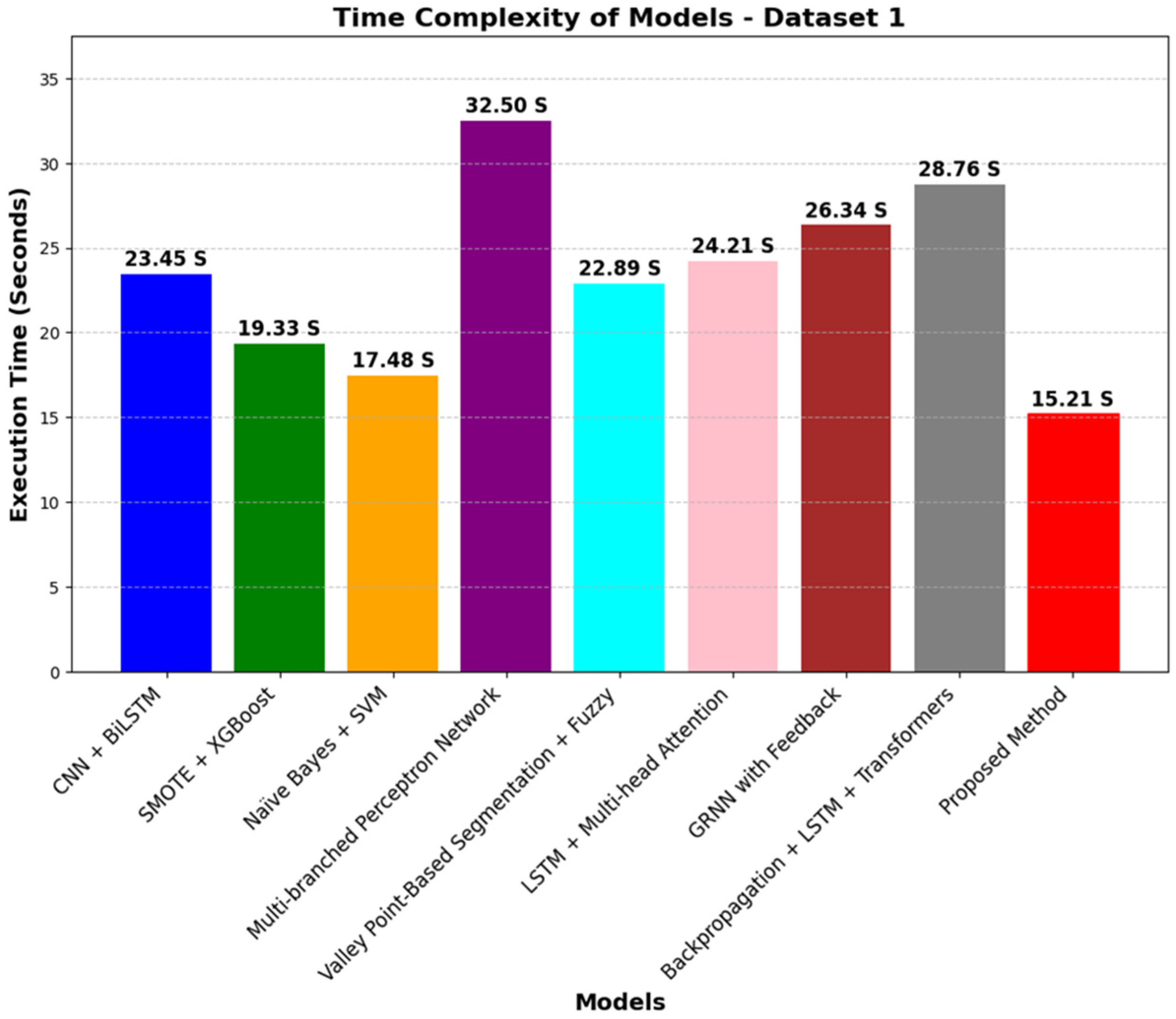
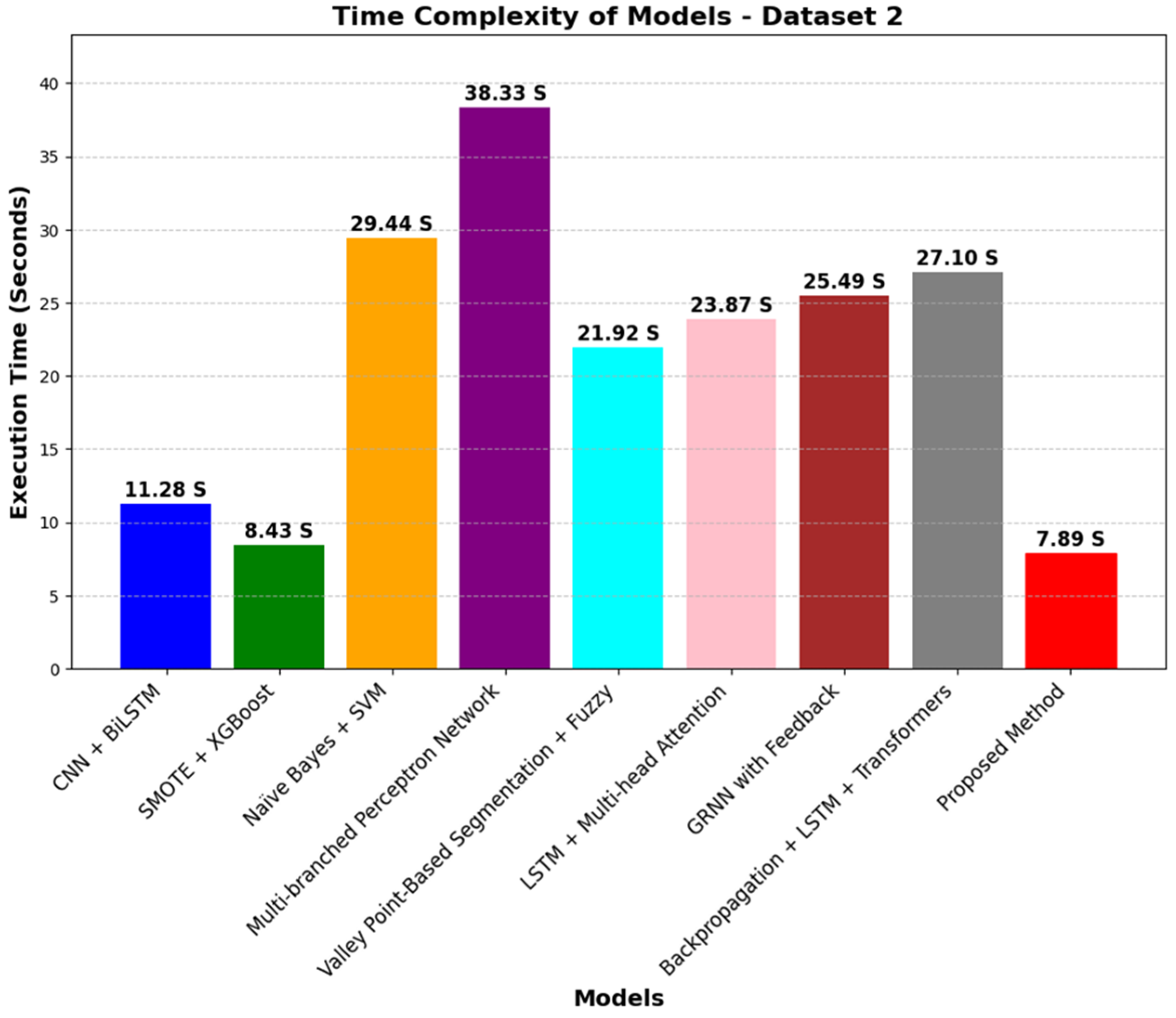
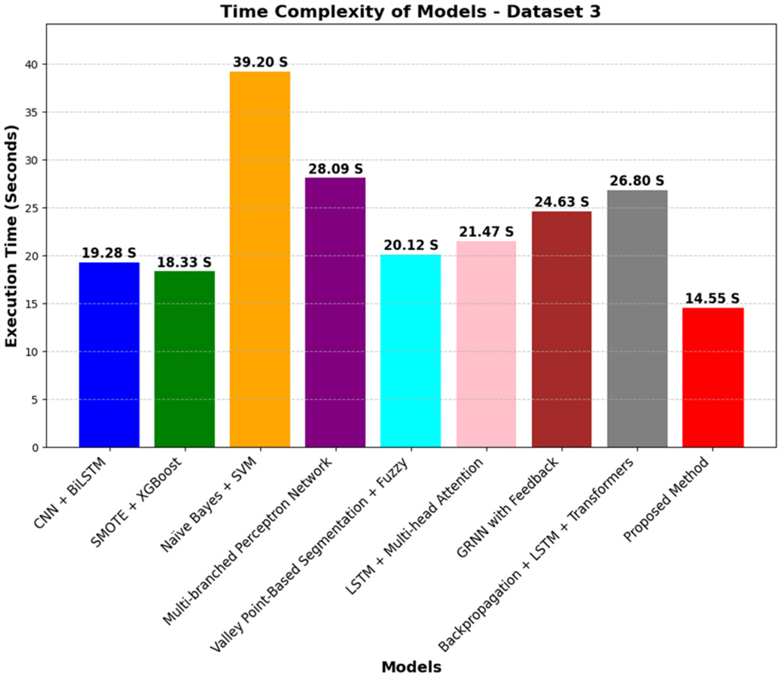
4.5.2. Time Complexity Comparison

Figure 10, Figure 11 and Figure 12 show a comparison of the time complexity of the proposed method versus other baseline models across three datasets. The CNN + BiLSTM model performs at moderate running times on all datasets. For Dataset 1, it operates at 23.45 s, indicating that although it adequately captures sequential dependence, additional processing complexity with the use of bidirectional LSTMs increases costs. In Dataset 2, it is markedly faster, at 11.28 s, hinting that the particular features in some datasets lower its cost of computation. For Dataset 3, its execution time is 19.28 s, which is relatively efficient in contrast to other deep learning models. The combination of bidirectional LSTMs and convolutional layers supports strong feature extraction and sequential learning but is not the most efficient in terms of time in this comparison.

The SMOTE + XGBoost model is uniformly one of the fastest for all the datasets. It has the lowest run time in Dataset 2, at 8.43 s, ranking it as the most computationally effective approach in this case. In Dataset 1, it runs for 19.33 s, and in Dataset 3, for 18.33 s, once again ranking among the fastest methods. The effectiveness of the SMOTE + XGBoost is due to its balanced strategy in dealing with imbalanced datasets and the light nature of Gradient Boosting, which is not computationally intensive like deep learning models are. This model is especially beneficial when fast processing is needed while having a high classification performance.

Naïve Bayes + an SVM exhibits inconsistent execution times over datasets. It is a fast model for Dataset 1 with an execution time of 17.48 s, as it has a straightforward probabilistic structure and only a moderate number of parameters. In Dataset 2, however, its execution time rises notably to 29.44 s, which reveals that it suffers from dataset-dependent complexities. In Dataset 3, it is the slowest among all the models, taking 39.20 s, which may be due to higher feature dimensionality or computationally costly kernel operations in the SVM. This indicates that although Naïve Bayes + an SVM is efficient in certain instances, in other datasets, it might not generalize well.

The Multibranched Perceptron Network is the most computationally costly technique in all datasets. It registers the longest execution times in Dataset 1 (32.50 s), Dataset 2 (38.33 s), and Dataset 3 (28.09 s). The higher computational cost is presumably because of its intricate architecture with multiple branches, deep layers, and residual connections, all of which contribute greatly to an increased execution time. Although such complexity could enhance accuracy in classification, it is computationally costly and hence inappropriate for real-time use or applications necessitating rapid model inference.

The Valley Point-Based Segmentation + fuzzy approach demonstrates a good balance between efficiency and complexity. On Dataset 1, it runs in 22.89 s, which is fairly efficient compared to the other deep learning-based methods. On Dataset 2, it runs in 21.92 s, indicating that it has a consistent computational cost. On Dataset 3, it runs in 20.12 s, further confirming its moderate run time. This approach takes advantage of fuzzy logic’s capability to deal with uncertainty in data at affordable computational costs. The LSTM + multi-head attention approach performs moderately on datasets with an execution time of 24.21 s for Dataset 1, 23.87 s for Dataset 2, and 21.47 s for Dataset 3. multi-head attention enables the model to attend to various regions of the input sequence at the same time, improving feature extraction. Nevertheless, the computational cost of attention the mechanisms and LSTMs adds to the execution time over more parsimonious models, such as the SMOTE + XGBoost. Though efficient in enhancing classification accuracy, this approach is not the most time-effective.

The GRNN with Feedback also has moderate execution times on datasets. For Dataset 1, its time is is 26.34 s; for Dataset 2, its time is 25.49 s; and for Dataset 3, its execution time is 24.63 s. GRNNs are fast learners, too, but computational complexity is involved in the Feedback Mechanism, and therefore, execution time is greater. Although this approach performs well in enhancing predictive performance, it is more computationally intensive compared to other models, such as the SMOTE + XGBoost and the current method. The Backpropagation + LSTM + Transformers approach incurs high computational costs on all datasets. Its times are 28.76 s in Dataset 1, 27.10 s in Dataset 2, and 26.80 s in Dataset 3. The combination of Backpropagation, LSTMs, and Transformers results in a colossal computational overhead because each one of them contributes to the execution time. Although transformers improve feature representation using self-attention mechanisms, transformers are computationally expensive, and, hence, this model is not fit for applications that involve low-latency inference.

The proposed method always has one of the shortest execution times on all the datasets. For Dataset 1, it executes at 15.21 s, which is the second shortest model time. For Dataset 2, it is the method with the shortest execution time of 7.89 s, proving its efficiency. For Dataset 3, it is still one of the quickest, executing in 14.55 s. The method in question balances computational effectiveness with architectural complexity and thus stands over computationally intensive models such as the Multibranched Perceptron Network and Backpropagation + LSTM + Transformers models with similar accuracy, although with greater computational costs. This indicates that it is promising for real-time scenario performance and contexts where the execution time is also a determining factor.

4.6. Research Limitations

The global results conclude that the proposed method provides a good trade-off between computational efficiency and model complexity and can compete in execution time on all datasets. Nevertheless, this study has some limitations that require further exploration.

• The computational demands of the proposed method, though moderate in comparison to the Multibranched Perceptron Network, are still more demanding than simple models such as the Smote + XGBoost and CNN + BiLSTM. Thus, the method requires optimization in terms of reducing execution time without the loss of performance, especially in real-time or resource-constrained applications.
• The performance of the proposed method was tested only on three datasets. Although the used datasets were heterogeneous, wider generalization can be achieved if more datasets are considered with various class imbalances, feature dimensions, and noise levels. This could confirm the robustness of the proposed method under even more challenging and diverse settings.
• This work mainly investigates execution time in terms of time complexity. Execution time analysis gives insight into the efficiency of computation but cannot account for memory consumption, energy consumption, and even scalability to larger datasets. Maybe it would be worthwhile to consider these as well, and thus broaden the understanding of whether the method has any computational feasibility.
• One of the main limitations of the proposed approach is its heavy dependence on hyperparameters. Performance depends on the appropriate tuning of many hyperparameters related to learning rates, optimization algorithms, and even architectural configurations. These hyperparameters do improve a model’s capability to adapt better to different datasets; however, at the same time, they raise the complexity associated with training this process and would possibly demand large computing resources for hyperparameter fine-tuning. It also limits the ease of deployment for the method since suboptimal hyperparameter settings can lead to significant performance degradation.
• Although the proposed method performs well, the architecture may still need further innovations, such as lightweight components, pruning techniques, or adaptive mechanisms that dynamically adjust the computational effort depending on the complexity of the dataset. These will help improve its applicability in dynamic and real-world environments.

Future work should cover these limitations and look into improving computational efficiency, expanding evaluation through other datasets and looking at different metrics that measure the overall performance and feasibility of the method.

4.7. Research Implications

The results of this research have important implications for the development of advanced machine learning frameworks that balance computational efficiency with predictive accuracy. In this context, the proposed approach addresses the limitations of the existing methods. It shows promise for practical applications in real-world scenarios where both performance and time complexity are critical factors.

Its robustness is its major strength, realized through the Tree Convolutional Neural Network (T-CNN), which accurately extracts high-granularity traffic patterns to detect minute anomalies that standard models tend to miss. In addition, the addition of a deep autoencoder increases the robustness of the framework to noise, such that key features are preserved for correct classification even in noisy network settings. Suitability is exhibited through the flexibility of the framework over diverse benchmark datasets (UNSW-NB15, CIC-IDS 2017, and CIC-IDS 2018). The approach generalizes effectively under differing network conditions, and thus is implementable in practical cybersecurity contexts. The inclusion of a Leader-Guided Velocity-Based Spiral Optimization method also ensures optimality by striking a balance between exploration and exploitation, resulting in a model performance with minimal computational expenditures.

A further important dimension is explainability, since the suggested method employs a systematic, interpretable anomaly detection mechanism. The hybrid optimization strategy provides a strong justification for parameter choice, while ensemble metaclassification maximizes decision transparency via prediction aggregation. Not only does the system enhance detection efficacy, but it also provides insights into anomaly types, which will benefit security analysts in grasping attack behaviors and mitigation techniques.

Compared with various models, this study develops a comprehensive framework for evaluating the trade-offs between execution time and architectural complexity, thus significantly growing knowledge on the topic of machine learning model selection and design. The work developed here will serve as a stepping stone to increase efficiency and robustness in future endeavors in such research lines toward more widespread industrial and academic usage of the related advanced machine learning technologies.

5. Conclusions and Future Scope

This research successfully demonstrates a novel approach to balancing computational efficiency and predictive accuracy through the introduction of a method that outperforms several baseline models in diverse datasets. Significant reductions in execution time are realized with robust performance, which makes the proposed method very adaptable and practically relevant for complex real-world applications. Compared to traditional methods, such as CNN + BiLSTM, Smote + XGBoost, and the Multibranched Perceptron Network, the proposed model strikes an optimal balance between time complexity and model performance, making it highly suitable for time-sensitive domains like network security, healthcare, and IoT systems.

The results not only focus on the role of architectural innovation but also call attention to optimizing model design with regard to meeting the computational needs of modern applications. The advanced feature extraction mechanism and dynamic learning strategy integrated within the proposed method form a starting point for future exploration into the design of efficient, scalable, and high-performing machine learning solutions. However, the proposed method has huge potential for future work. Some directions that are worth researching include the following: the application of adaptive and automated hyperparameter-tuning techniques, such as reinforcement learning or Bayesian optimization, which will avoid the deterministic manual selection process and hence enhance the robustness of models and their ease of deployment in various environments.

Furthering the extent of the evaluation of the proposed method via bigger and more complex datasets and domains, with varied characteristics such as multi-modal data, imbalanced datasets, and high-dimensional inputs, will strengthen its generalizability. The use of lightweight components such as pruning mechanisms or the integration of quantization techniques may also improve computational efficiency. Hybrid methodologies could achieve further improvements in performance through the integration of the proposed approach with advanced metaheuristic optimization algorithms. Moreover, new studies can investigate cost-minimized multi-stage optimization models [48] to improve the efficiency of anomaly detection systems further. These improvements may explore how analogous dynamic cost-sensitive optimization approaches can be utilized in cybersecurity. Such approaches would help optimize the learning process’s efficiency, particularly in high-dimensional datasets or in cases where adaptation to changing input conditions is dynamic.

Future work can involve further extending the method’s applicability to the scenario of streaming data, wherein the model would have to adjust dynamically according to the input streams without any retraining. Techniques for continual learning or incremental learning might be added to maintain the effectiveness of the model over time. Finally, the model may be incorporated with strong security mechanisms, like blockchain-based data validation and Explainable AI anomaly detection through distributed learning frameworks, which could further increase the practical applicability of this method in critical domains like cybersecurity and fraud detection.

References

1. Djenna, A.; Harous, S.; Saidouni, D.E. Internet of things meet internet of threats: New concern cyber security issues of critical cyber infrastructure. Appl. Sci. 2021, 11, 4580. [Google Scholar] [CrossRef]
2. Ani, U.P.D.; He, H.; Tiwari, A. Review of cybersecurity issues in industrial critical infrastructure: Manufacturing in perspective. J. Cyber Secur. Technol. 2017, 1, 32–74. [Google Scholar] [CrossRef]
3. Shroff, J.; Walambe, R.; Singh, S.K.; Kotecha, K. Enhanced security against volumetric DDoS attacks using adversarial machine learning. Wirel. Commun. Mob. Comput. 2022, 2022, 5757164. [Google Scholar] [CrossRef]
4. Hassan, A.I.; El Reheem, E.A.; Guirguis, S.K. An entropy and machine learning based approach for DDoS attacks detection in software defined networks. Sci. Rep. 2024, 14, 18159. [Google Scholar] [CrossRef]
5. Tang, K.H.; Ghanem, M.C.; Vassilev, V.; Ouazzane, K.; Gasiorowski, P. Synchronization, Optimization, and Adaptation of Machine Learning Techniques for Computer Vision in Cyber-Physical Systems: A Comprehensive Analysis. Preprints 2025, 2025010521. [Google Scholar] [CrossRef]
6. Al-Khayyat, A.T.K.; Ucan, O.N. A Multi-Branched Hybrid Perceptron Network for DDoS Attack Detection Using Dynamic Feature Adaptation and Multi-Instance Learning. IEEE Access 2024, 12, 192618–192638. [Google Scholar] [CrossRef]
7. Malliga, S.; Nandhini, P.S.; Kogilavani, S.V. A comprehensive review of deep learning techniques for the detection of (distributed) denial of service attacks. Inf. Technol. Control 2022, 51, 180–215. [Google Scholar] [CrossRef]
8. Gwassi, O.A.H.; Uçan, O.N.; Navarro, E.A. Cyber-XAI-Block: An end-to-end cyber threat detection & fl-based risk assessment framework for iot enabled smart organization using xai and blockchain technologies. Multimed. Tools Appl. 2024, 1–42. [Google Scholar] [CrossRef]
9. Alotaibi, A.; Rassam, M.A. Adversarial machine learning attacks against intrusion detection systems: A survey on strategies and defense. Future Internet 2023, 15, 62. [Google Scholar] [CrossRef]
10. Yin, D.; Zhang, L.; Yang, K. A DDoS attack detection and mitigation with software-defined Internet of Things framework. IEEE Access 2018, 6, 24694–24705. [Google Scholar] [CrossRef]
11. Khatri, A.; Khatri, R. DDoS Attack Detection Using Artificial Neural Network on IoT Devices in a Simulated Environment. In International Conference on IoT, Intelligent Computing and Security: Select Proceedings of IICS 2021; Springer Nature: Singapore, 2023; pp. 221–233. [Google Scholar]
12. Parmar, A.; Lamkuche, H. Distributed Denial of Service Attack Detection Using Sequence-To-Sequence LSTM. In Proceedings of the International Conference on Global Economic Revolutions, Sharjah, United Arab Emirates, 27–28 February 2023; Springer Nature: Cham, Switzerland, 2023; pp. 39–53. [Google Scholar]
13. Wang, J.; Wang, L.; Wang, R. A Method of DDoS Attack Detection and Mitigation for the Comprehensive Coordinated Protection of SDN Controllers. Entropy 2023, 25, 1210. [Google Scholar] [CrossRef]
14. Bala, B.; Behal, S. AI techniques for IoT-based DDoS attack detection: Taxonomies, comprehensive review and research challenges. Comput. Sci. Rev. 2024, 52, 100631. [Google Scholar] [CrossRef]
15. Hnamte, V.; Najar, A.A.; Nhung-Nguyen, H.; Hussain, J.; Sugali, M.N. DDoS attack detection and mitigation using deep neural network in SDN environment. Comput. Secur. 2024, 138, 103661. [Google Scholar] [CrossRef]
16. Anley, M.B.; Genovese, A.; Agostinello, D.; Piuri, V. Robust DDoS attack detection with adaptive transfer learning. Comput. Secur. 2024, 144, 103962. [Google Scholar] [CrossRef]
17. Zhao, J.; Liu, Y.; Zhang, Q.; Zheng, X. CNN-AttBiLSTM Mechanism: A DDoS Attack Detection Method Based on Attention Mechanism and CNN-BiLSTM. IEEE Access 2023, 11, 136308–136317. [Google Scholar] [CrossRef]
18. Presekal, A.; Ştefanov, A.; Semertzis, I.; Palensky, P. Spatio-Temporal Advanced Persistent Threat Detection and Correlation for Cyber-Physical Power Systems using Enhanced GC-LSTM. IEEE Trans. Smart Grid 2024, 16, 1654–1666. [Google Scholar] [CrossRef]
19. Aktar, S.; Nur, A.Y. Robust Anomaly Detection in IoT Networks using Deep SVDD and Contractive Autoencoder. In Proceedings of the 2024 IEEE International Systems Conference (SysCon), Montreal, QC, Canada, 15–18 April 2024; IEEE: New York, NY, USA, 2024; pp. 1–8. [Google Scholar]
20. Jiyad, Z.M.; Al Maruf, A.; Haque, M.M.; Gupta, M.S.; Ahad, A.; Aung, Z. DDoS Attack Classification Leveraging Data Balancing and Hyperparameter Tuning Approach Using Ensemble Machine Learning with XAI. In Proceedings of the 2024 Third International Conference on Power, Control and Computing Technologies (ICPC2T), Raipur, India, 18–20 January 2024; IEEE: New York, NY, USA, 2024; pp. 569–575. [Google Scholar]
21. Qaddos, A.; Yaseen, M.U.; Al-Shamayleh, A.S.; Imran, M.; Akhunzada, A.; Alharthi, S.Z. A novel intrusion detection framework for optimizing IoT security. Sci. Rep. 2024, 14, 21789. [Google Scholar] [CrossRef]
22. Sajid, M.; Malik, K.R.; Almogren, A.; Malik, T.S.; Khan, A.H.; Tanveer, J.; Rehman, A.U. Enhancing intrusion detection: A hybrid machine and deep learning approach. J. Cloud Comput. 2024, 13, 123. [Google Scholar] [CrossRef]
23. Ye, Z.; Luo, J.; Zhou, W.; Wang, M.; He, Q. An ensemble framework with improved hybrid breeding optimization-based feature selection for intrusion detection. Future Gener. Comput. Syst. 2024, 151, 124–136. [Google Scholar] [CrossRef]
24. Kumar, G.S.C.; Kumar, R.K.; Kumar, K.P.V.; Sai, N.R.; Brahmaiah, M. Deep residual convolutional neural network: An efficient technique for intrusion detection system. Expert Syst. Appl. 2024, 238, 121912. [Google Scholar] [CrossRef]
25. Moustafa, N.; Slay, J. UNSW-NB15: A comprehensive data set for network intrusion detection systems (UNSW-NB15 network data set). In Proceedings of the 2015 Military Communications and Information Systems Conference (MilCIS), Canberra, ACT, Australia, 10–12 November 2015; IEEE: New York, NY, USA, 2015; pp. 1–6. [Google Scholar]
26. Sharafaldin, I.; Lashkari, A.H.; Ghorbani, A.A. Toward generating a new intrusion detection dataset and intrusion traffic characterization. ICISSp 2018, 1, 108–116. [Google Scholar]
27. Leevy, J.L.; Khoshgoftaar, T.M. A survey and analysis of intrusion detection models based on CSE-CIC-IDS2018 big data. J. Big Data 2020, 7, 104. [Google Scholar] [CrossRef]
28. Duan, B. The Robustness of Trimming and Winsorization When the Population Distribution Is Skewed. Ph.D. Dissertation, Tulane University, New Orleans, LA, USA, 1998. [Google Scholar]
29. Feng, C.; Wang, H.; Lu, N.; Chen, T.; He, H.; Lu, Y.; Tu, X.M. Log-transformation and its implications for data analysis. Shanghai Arch. Psychiatry 2014, 26, 105. [Google Scholar] [PubMed]
30. Shanker, M.; Hu, M.Y.; Hung, M.S. Effect of data standardization on neural network training. Omega 1996, 24, 385–397. [Google Scholar] [CrossRef]
31. Patro, S.G.; Sahu, K.K. Normalization: A preprocessing stage. arXiv 2015, arXiv:1503.06462. [Google Scholar] [CrossRef]
32. Biswas, B.; Ghosh, S.K.; Ghosh, A. DVAE: Deep variational auto-encoders for denoising retinal fundus image. In Hybrid Machine Intelligence for Medical Image Analysis; Springer Nature: Cham, Switzerland, 2020; pp. 257–273. [Google Scholar]
33. Shi, Y.; Eberhart, R.C. Empirical study of particle swarm optimization. In Proceedings of the 1999 Congress on Evolutionary Computation-CEC99 (Cat. No. 99TH8406), Washington, DC, USA, 6–9 July 1999; IEEE: New York, NY, USA, 1999; Volume 3, pp. 1945–1950. [Google Scholar]
34. Trojovský, P.; Dehghani, M. Pelican optimization algorithm: A novel nature-inspired algorithm for engineering applications. Sensors 2022, 22, 855. [Google Scholar] [CrossRef]
35. Taşcı, E. A meta-ensemble classifier approach: Random rotation forest. Balkan J. Electr. Comput. Eng. 2019, 7, 182–187. [Google Scholar] [CrossRef]
36. Joachims, T. SVMlight: Support vector machine. SVM-Light Support Vector Mach. 1999, 19, 25. [Google Scholar]
37. Wickramasinghe, I.; Kalutarage, H. Naive Bayes: Applications, variations and vulnerabilities: A review of literature with code snippets for implementation. Soft Comput. 2021, 25, 2277–2293. [Google Scholar] [CrossRef]
38. Salman, H.A.; Kalakech, A.; Steiti, A. Random forest algorithm overview. Babylonian J. Mach. Learn. 2024, 2024, 69–79. [Google Scholar] [CrossRef]
39. Yadav, S.; Shukla, S. Analysis of k-fold cross-validation over hold-out validation on colossal datasets for quality classification. In Proceedings of the 2016 IEEE 6th International Conference on Advanced Computing (IACC), Bhimavaram, India, 27–28 February 2016; IEEE: New York, NY, USA, 2016; pp. 78–83. [Google Scholar]
40. Susmaga, R. Confusion Matrix Visualization. In Intelligent Information Processing and Web Mining: Proceedings of the International IIS: IIPWM ‘04 Conference Held in Zakopane, Poland, 17–20 May 2004; Springer: Berlin/Heidelberg, Germany, 2004; pp. 107–116. [Google Scholar]
41. Buckland, M.; Gey, F. The relationship between recall and precision. J. Am. Soc. Inf. Sci. 1994, 45, 12–19. [Google Scholar] [CrossRef]
42. Zhang, R.; Zhan, J.; Ding, W.; Pedrycz, W. Time series fore casting based on improved multi-linear trend fuzzy information granules for convolutional neural networks. IEEE Trans. Fuzzy Syst. 2024, 33, 1009–1023. [Google Scholar] [CrossRef]
43. Gu, J.; Lu, S. An effective intrusion detection approach using SVM with naïve Bayes feature embedding. Comput. Secur. 2021, 103, 102158. [Google Scholar] [CrossRef]
44. Wu, X.; Zhan, J.; Ding, W.; Pedrycz, W. GRNN Model with Feedback Mechanism Incorporating kkk-Nearest Neighbor and Modified Gray Wolf Optimization Algorithm in Intelligent Transportation. IEEE Trans. Intell. Transp. Syst. 2024, 26, 3855–3872. [Google Scholar] [CrossRef]
45. Talukder, M.A.; Islam, M.M.; Uddin, M.A.; Hasan, K.F.; Sharmin, S.; Alyami, S.A.; Moni, M.A. Machine learning-based network intrusion detection for big and imbalanced data using oversampling, stacking feature embedding and feature extraction. J. Big Data 2024, 11, 33. [Google Scholar] [CrossRef]
46. Cai, M.; Zhan, J.; Zhang, C.; Liu, Q. Fusion k-means clustering and multi-head self-attention mechanism for a multivariate time prediction model with feature selection. Int. J. Mach. Learn. Cybern. 2024, 1–19. [Google Scholar] [CrossRef]
47. Zhu, C.; Ma, X.; D’Urso, P.; Qian, Y.; Ding, W.; Zhan, J. Long-term multivariate time series forecasting model based on Gaussian fuzzy information granules. IEEE Trans. Fuzzy Syst. 2024, 263, 125705. [Google Scholar] [CrossRef]
48. Zhan, J.; Cai, M. A cost-minimized two-stage three-way dynamic consensus mechanism for social network-large scale group decision-making: Utilizing K-nearest neighbors for incomplete fuzzy preference relations. Expert Syst. Appl. 2025, 263, 125705. [Google Scholar] [CrossRef]
Figure 1. Architecture of proposed intrusion detection model.
Symmetry 17 00421 g001
Figure 2. The architecture of the proposed Tree Convolutional Neural Network.
Symmetry 17 00421 g002
Figure 3. The architecture of the Variational Wavelet Autoencoder.
Symmetry 17 00421 g003
Figure 4. Layout of confusion matrix.
Symmetry 17 00421 g004
Figure 5. Epoch-wise performance of proposed hybrid architecture in terms of classification accuracy (a) and loss (b).
Symmetry 17 00421 g005
Figure 6. Confusion matrix (a) and ROC curve (b) of the proposed architecture for Dataset 1 (UNSW-NB15 dataset).
Symmetry 17 00421 g006
Figure 7. Epoch-wise performance of proposed hybrid architecture in terms of classification accuracy (a), loss (b), confusion matrix (c), and ROC curve (d) for Dataset 2 (CICIDS-2017 dataset).
Symmetry 17 00421 g007
Figure 8. Epoch-wise performance of proposed hybrid architecture in terms of classification accuracy (a) and loss (b).
Symmetry 17 00421 g008
Figure 9. Confusion matrix (a) and ROC curve (b) of proposed architecture for Dataset 3 (CICIDS-2018 dataset).
Symmetry 17 00421 g009
Figure 10. Time complexity comparison for Dataset 1.
Symmetry 17 00421 g010
Figure 11. Time complexity comparison for Dataset 2.
Symmetry 17 00421 g011
Figure 12. Time complexity comparison for Dataset 3.
Symmetry 17 00421 g012