Development and Engineering Applications of a Novel Mixture Distribution: Exponentiated and New Topp–Leone-G Families

Abstract

In this paper, two different families are mixed: the exponentiated and new Topp–Leone-G families. This yields a new family, which we named the mixture of the exponentiated and new Topp–Leone-G family. Some statistical properties of the proposed family are obtained. Then, the mixture of two exponentiated new Topp–Leone inverse Weibull distribution is introduced as a sub-model from the mixture of exponentiated and new Topp–Leone-G family. Some related properties are studied, such as the quantile function, moments, moment generating function, and order statistics. Furthermore, the maximum likelihood and Bayes approaches are employed to estimate the unknown parameters, reliability and hazard rate functions of the mixture of exponentiated and new Topp–Leone inverse Weibull distribution. Bayes estimators are derived under both the symmetric squared error loss function and the asymmetric linear exponential loss function. The performance of maximum likelihood and Bayes estimators is evaluated through a Monte Carlo simulation. The applicability and flexibility of the MENTL-IW distribution are demonstrated by well-fitting two real-world engineering datasets. The results demonstrate the superior performance of the MENTL-IW distribution compared to other competing models.

1. Introduction

Finite mixture distributions are widely used in medical, engineering and scientific applications to model heterogeneous data more effectively. In these situations, the population may consist of components, each potentially following a different distribution or the same distribution but with different parameters. This results in a mixture of components, where each component has its own unique probability density function (pdf).

Therefore, a finite mixture distribution can be defined as a probability distribution resulting from a weighted combination of two or more component distributions. These components may result from the same distribution with different parameters or from different distributions. The mixing proportions determine the relative contribution of each component to the mixture.

The pdf and the cumulative distribution function (cdf) for the mixture of two components’ densities with mixing proportions ($p_i, i=\mathrm{1,2}$), respectively, are

$$f\left(x\right)=\sum _{i=1}^2{p}_i{g}_i\left(x\right),$$

(1)

and

$$F\left(x\right)=\sum _{i=1}^2{p}_i{G}_i\left(x\right),$$

(2)

where $p_i$ are the mixing proportions satisfying the conditions $\sum _{i=1}^2{p}_i=1$ and ${0\le p}_i\le 1$.

Mixture distributions have attracted attention from researchers across various scientific and practical domains. For example, Ref. [1] obtained approximate Bayes estimators for the parameters of a mixture of two Weibull distributions under Type-II censoring. Ref. [2] investigated the statistical properties of a finite mixture of two Gompertz lifetime models. Ref. [3] employed both the maximum likelihood (ML) and Bayesian approaches to estimate the parameters of a finite mixture of two exponential distributions based on record statistics. Ref. [4] utilized both ML and Bayesian methods to estimate the parameters, reliability function (rf), and hazard rate function (hrf) of two-component finite mixtures of exponentiated gamma distributions.

In recent years, research on mixture models has seen significant advancements. For example, Ref. [5] introduced a mixture of the Marshall–Olkin extended Weibull distributions for effective modeling failure, survival, and COVID-19 data under both non-Bayesian and Bayesian approaches, considering Type-II censored data. Ref. [6] developed a method based on quantiles to estimate the parameters of a finite mixture of Fréchet distributions for large samples of dependent data. More recently, Ref. [7] proposed a new family of continuous distributions by considering a mixture of two components from the exponentiated family.

Finite mixture models constitute a well-developed area of statistical research, with applications covering various fields. Ref. [8] introduced a thorough overview of finite mixture models, containing their theoretical establishments, estimation methods, and practical applications. This important work highlights the flexibility of finite mixture models in capturing complex data structures and their ability to model heterogeneity within a population. By examining a wide range of mixture models, including those with multiple components, they provide valuable insights into the challenges and opportunities associated with modeling complex data using finite mixture approaches.

Ref. [9] investigated the identifiability and estimation of mixtures of extreme-value distributions. Their work provides a base for understanding the challenges and complexities associated with estimating parameters in multi-component mixture models. While they focused specifically on extreme-value distributions, they highlighted the importance of considering identifiability issues and the development of robust estimation techniques when dealing with complex mixture models.

The fundamental motivation of this paper is to introduce a novel mixture family of distributions. This new family is constructed by combining the exponentiated family, introduced by [10], with the new Topp–Leone-G (NTL-G) family proposed by [11]. This approach aims to generate a wide range of flexible mixture distributions for modeling various real-world phenomena.

The pdf and cdf of the exponentiated family are

$$f\left(x\right)=\alpha g\left(x\right){\left[G\left(x\right)\right]}^{\alpha -1}, x\in \mathbb{R},$$

(3)

and

$$F\left(x\right)={\left[G\left(x\right)\right]}^{\alpha },$$

(4)

where $\alpha >0$ is a shape parameter, and $g\left(x\right) \mathrm{a}\mathrm{n}\mathrm{d} G\left(x\right)$ are the pdf and cdf of the baseline distribution, respectively.

The pdf and cdf of the new Topp–Leone-G family are defined as

$$f\left(x;\alpha \right)={\displaystyle \frac{2\alpha g\left(x\right)}{{\left[1-G\left(x\right)\right]}^2}}{e}^{-2H\left(x\right)}{\left(1-e^{-2H\left(x\right)}\right)}^{\alpha -1}, x\in \mathbb{R},$$

(5)

and

$$F\left(x;\alpha \right)={\left(1-e^{-2H\left(x\right)}\right)}^{\alpha },$$

(6)

where $H\left(x\right)={\displaystyle \frac{G\left(x\right)}{1-G\left(x\right)}}$ is the odds ratio.

This paper is organized as follows: Section 2 introduces the mixture of exponentiated and NTL-G (MENTL-G) family of distributions and discusses some of its statistical properties. In Section 3, the MENTL inverse Weibull (MENTL-IW) distribution is presented as a specific sub-model within the MENTL-G family, along with the derivation of some of its statistical properties. Outlines of the methodologies used for parameter estimation are proposed in Section 4, including both the maximum likelihood (ML) and Bayesian approaches. Section 5 introduces a simulation study to evaluate the performance of the ML and Bayesian estimators for the parameters of the MENTL-IW distribution. Finally, Section 6 demonstrates the flexibility and applicability of the proposed distribution by applying it to two real-world datasets.

2. Mixture of Exponentiated and New Topp Leone-G Family

The pdf for the MENTL-G family can be obtained by substituting (3) and (5) in (1) with mixing proportion $p$ and $(1-p)$ as follows:

$$f\left(x\right)=p\alpha g_1\left(x\right){\left[G_1\left(x\right)\right]}^{\alpha -1}+{\displaystyle \frac{2(1-p)\beta g_2\left(x\right)}{{\left[1-G_2\left(x\right)\right]}^2}}{e}^{-2H\left(x\right)}{\left[1-e^{-2H\left(x\right)}\right]}^{\beta -1},x>0,\alpha ,\beta >0,$$

(7)

where $g_1\left(x\right)$ and $G_1\left(x\right)$ are the pdf and cdf of the baseline distribution for the first component, respectively. Also, $g_2\left(x\right)$ and $G_2\left(x\right)$ are the pdf and cdf of the baseline distribution for the second component, respectively.

Then, the cdf of MENTL-G family is

$$F\left(x\right)=p{\left[G_1\left(x\right)\right]}^{\alpha }+\left(1-p\right){\left[1-e^{-2H\left(x\right)}\right]}^{\beta }, x>0, \alpha ,\beta >0,$$

(8)

where $H\left(x\right)={\displaystyle \frac{G_2\left(x\right)}{1-G_2\left(x\right)}}$.

The corresponding rf, hrf, and reversed hazard rate function (rhrf) of the MENTL-G family are

$$S\left(x\right)=1-p{\left[G_1\left(x\right)\right]}^{\alpha }-\left(1-p\right){\left[1-e^{-2H\left(x\right)}\right]}^{\beta }, x>0, \alpha ,\beta >0,$$

(9)

$$h\left(x\right)={\displaystyle \frac{p\alpha g_1\left(x\right){\left[G_1\left(x\right)\right]}^{\alpha -1}+\frac{2\left(1-p\right)\beta g_2\left(x\right)}{{\left[1-G_2\left(x\right)\right]}^2}{e}^{-2H\left(x\right)}{\left[1-e^{-2H\left(x\right)}\right]}^{\beta -1}}{1-p{\left[G_1\left(x\right)\right]}^{\alpha }-\left(1-p\right){\left[1-e^{-2H\left(x\right)}\right]}^{\beta }}}, x>0, \alpha ,\beta >0,$$

(10)

and

$$rh\left(x\right)={\displaystyle \frac{p\alpha g_1\left(x\right){\left[G_1\left(x\right)\right]}^{\alpha -1}+\frac{2(1-p)\beta g_2\left(x\right)}{{\left[1-G_2\left(x\right)\right]}^2}{e}^{-2H\left(x\right)}{\left[1-e^{-2H\left(x\right)}\right]}^{\beta -1}}{p{\left[G_1\left(x\right)\right]}^{\alpha }+\left(1-p\right){\left[1-e^{-2H\left(x\right)}\right]}^{\beta }}}$$

(11)

2.1. General Properties of the Mixture of Exponentiated and New Topp–Leone-G Families

In this subsection, various properties of the MENTL-G family are described.

2.1.1. Quantile Function of the MENTL-G Family

The quantile function of the MENTL-G family can be derived from (8) by solving $Q\left(u\right)=F^{-1}\left(u\right)$, i.e., $F\left(x\right)=u$ for $x$, as given below.

$$\mathit{ln}\left\{p{\left[G_1\left(x_u\right)\right]}^{\alpha }+\left(1-p\right){\left[1-e^{-2H\left(x_u\right)}\right]}^{\beta }\right\}-\mathit{ln}u=0, 0<u<1.$$

(12)

Then, to obtain the uth quantile for the MENTL-G random variable, Equation (12) should be solved numerically.

2.1.2. Moments of the MENTL-G Family

The rth moment about the origin of the MENTL-G family is obtained using (7) as follows:

$$\begin{array}{l}{\mu }_r^{\prime }=E\left(x^r\right)\\ ={\displaystyle \sum _{j=1}^2}{p}_j{E}_j\left(x^r\right)\\ =p{E}_1\left(x^r\right)+\left(1-p\right)E_2\left(x^r\right)\\ =p\alpha {\int }_0^{\infty }{x}^r{g}_1\left(x\right){\left[G_1\left(x\right)\right]}^{\alpha -1}dx\\ +2\left(1-p\right)\beta {\int }_0^{\infty }{x}^r{\displaystyle \frac{g_2\left(x\right)}{{\left[1-G_2\left(x\right)\right]}^2}}{e}^{-2H\left(x\right)}{\left[1-e^{-2H\left(x\right)}\right]}^{\beta -1}dx.\end{array}$$

Considering the following sequences:

• The series’ representation as $a^x=\sum _{i=0}^{\mathrm{\infty }}{\displaystyle \frac{{\left(\mathit{ln}a\right)}^i}{i!}}{x}^i$;
• The generalized binomial expansion for $n>0$ is a real non-integer

  $${\left(1-x\right)}^n={\sum }_{i=0}^{\mathrm{\infty }}{\left(-1\right)}^i\left({\displaystyle \genfrac{}{}{0pt}{}{n}{i}}\right)x^i,\left|x\right|<1;$$
• Taylor expansion $e^x=\sum _{j=0}^{\mathrm{\infty }}{\displaystyle \frac{x^j}{j!}}$.

Then, the rth moment of the MENTL-G family is

$${\mu }_r^{\prime }=\sum _{j_1=0}^{\infty }{\displaystyle \frac{{\left(\alpha -1\right)}^{j_1}}{j_1!}}{\phi }_{j_1,r}+\sum _{j_2=0}^{\infty } \sum _{j_3=0}^{\infty }{\left(-1\right)}^{j_2}{\left(-2\right)}^{j_3}\left({\displaystyle \genfrac{}{}{0pt}{}{\beta -1}{j_2}}\right){\displaystyle \frac{{\left(1+j_2\right)}^{j_3}}{j_3!}}{\phi }_{j_3,r},$$

(13)

where

$${\phi }_{j_1,r}=p\alpha {\int }_0^{\infty }{x}^r{g}_1\left(x\right){\left[{lnG}_1\left(x\right)\right]}^{j_1}dx,$$

and

$${\phi }_{j_3,r}=2\left(1-p\right)\beta {\int }_0^{\infty }{x}^r{\displaystyle \frac{g_2\left(x\right)}{{\left[1-G_2\left(x\right)\right]}^2}}{\left[H\left(x\right)\right]}^{j_3}dx.$$

2.1.3. Moment-Generating Function of the MENTL-G Family

The moment-generating function of the MENTL-G family is given by

$$M_x\left(t\right)=E\left(e^{tx}\right)={\int }_0^{\infty }{e}^{tx}f\left(x\right)dx=\sum _{r=0}^{\infty }{\displaystyle \frac{t^r}{r!}}{\mu }_r^{\prime },$$

(14)

where ${\mu }_r^{\prime }$ is the rth moment in (13), then the moment-generating function can be derived as follows:

$$M_x\left(t\right)=\sum _{r=0}^{\infty }{\displaystyle \frac{t^r}{r!}}\left[\begin{array}{c}{\displaystyle \sum _{j_1=0}^{\infty }}{\displaystyle \frac{{\left(\alpha -1\right)}^{j_1}}{j_1!}}{\phi }_{j_1,r}\\ +{\displaystyle \sum _{j_2=0}^{\infty }} {\displaystyle \sum _{j_3=0}^{\infty }}{\left(-1\right)}^{j_2}{\left(-2\right)}^{j_3}\left({\displaystyle \genfrac{}{}{0pt}{}{\beta -1}{j_2}}\right){\displaystyle \frac{{\left(1+j_2\right)}^{j_3}}{j_3!}}{\phi }_{j_3,r}\end{array}\right]$$

(15)

2.1.4. Order Statistics of the MENTL-G Family

The pdf of the ith order statistic from a random sample of size $n$ drawn from the MENTL-G family can be expressed as

$$\begin{array}{ll}{f}_{i,n}\left(x\right)& ={\displaystyle \sum _{k=0}^{n-i}}{\displaystyle \frac{n!{\left(-1\right)}^k}{\left(i-1\right)!k!\left(n-i-k\right)!}}\\ & \times \left(p\alpha g_1\left(x\right){\left[G_1\left(x\right)\right]}^{\alpha -1}+{\displaystyle \frac{2\left(1-p\right)\beta g_2\left(x\right)}{{\left[1-G_2\left(x\right)\right]}^2}}{e}^{-2H\left(x\right)}{\left[1-e^{-2H\left(x\right)}\right]}^{\beta -1}\right)\\ & \times {\left(p{\left[G_1\left(x\right)\right]}^{\alpha }+\left(1-p\right){\left[1-e^{-2H\left(x\right)}\right]}^{\beta }\right)}^{\left(i+k-1\right)}\end{array}$$

(16)

By substituting $i=1$ and $i=n$ into (16), one can obtain the pdfs of the smallest and largest order statistics, respectively.

3. Mixture of Two Exponentiated New Topp–Leone Inverse Weibull Distribution

In this section, the mixture of two ENTL-IW (MENTL-IW) distributions is considered as a sub-model from the MENTL-G family. Some statistical properties and estimations of the unknown parameters for the MENTL-IW are studied.

3.1. Description of the Distribution

If the pdf and cdf of the inverse Weibull (IW) distribution are

$$g\left(x;\lambda ,\gamma \right)=\lambda \gamma x^{-\left(\gamma +1\right)}{e}^{-\lambda x^{-\gamma }}, x>0,\lambda ,\gamma >0$$

(17)

and

$$G\left(x;\lambda ,\gamma \right)=e^{-\lambda x^{-\gamma }},$$

(18)

$\lambda$ is a scale parameter and $\gamma$ is a shape parameter.

The MENTL-IW distribution is derived by replacing the corresponding components in (7) with the pdf and cdf of the IW distribution, which are defined in (17) and (18), respectively.

The pdf of the MENTL-IW distribution is given by

$$\begin{array}{ll}{f}_M\left(x\right)& =p\alpha {\lambda }_1{\gamma }_1{x}^{-\left({\gamma }_1+1\right)}{e}^{-{\lambda }_1\alpha x^{-{\gamma }_1}}\\ & +2\beta {\lambda }_2{\gamma }_2(1-p)x^{-\left({\gamma }_2+1\right)}{e}^{-{\lambda }_2{x}^{-{\gamma }_2}-2{\displaystyle \frac{e^{-{\lambda }_2{x}^{-{\gamma }_2}}}{1-e^{-{\lambda }_2{x}^{-{\gamma }_2}}}}}{\displaystyle \frac{{\left[1-e^{-2\frac{e^{-{\lambda }_2{x}^{-{\gamma }_2}}}{1-e^{-{\lambda }_2{x}^{-{\gamma }_2}}}}\right]}^{\beta -1}}{{\left(1-e^{-{\lambda }_2{x}^{-{\gamma }_2}}\right)}^2}}\end{array}$$

(19)

The corresponding cdf, rf, hrf and rhrf of the MENTL-IW distribution are

$$F_M\left(x\right)=p{e}^{-{\lambda }_1\alpha x^{-{\gamma }_1}}+\left(1-p\right){\left[1-e^{-2{\displaystyle \frac{e^{-{\lambda }_2{x}^{-{\gamma }_2}}}{1-e^{-{\lambda }_2{x}^{-{\gamma }_2}}}}}\right]}^{\beta },$$

(20)

$$S_M\left(x\right)=1-p{e}^{-{\lambda }_1\alpha x^{-{\gamma }_1}}-\left(1-p\right){\left[1-e^{-2{\displaystyle \frac{e^{-{\lambda }_2{x}^{-{\gamma }_2}}}{1-e^{-{\lambda }_2{x}^{-{\gamma }_2}}}}}\right]}^{\beta },$$

(21)

$$h_M\left(x\right)={\displaystyle \frac{p\alpha {\lambda }_1{\gamma }_1{x}^{-\left({\gamma }_1+1\right)}{e}^{-{\lambda }_1\alpha x^{-{\gamma }_1}}+2\beta {\lambda }_2{\gamma }_2\left(1-p\right)x^{-\left({\gamma }_2+1\right)}{e}^{-{\lambda }_2{x}^{-{\gamma }_2}-2\frac{e^{-{\lambda }_2{x}^{-{\gamma }_2}}}{1-e^{-{\lambda }_2{x}^{-{\gamma }_2}}}}\frac{{\left[1-e^{-2\frac{e^{-{\lambda }_2{x}^{-{\gamma }_2}}}{1-e^{-{\lambda }_2{x}^{-{\gamma }_2}}}}\right]}^{\beta -1}}{{\left(1-e^{-{\lambda }_2{x}^{-{\gamma }_2}}\right)}^2}}{1-p{e}^{-{\lambda }_1\alpha x^{-{\gamma }_1}}-\left(1-p\right){\left[1-e^{-2\frac{e^{-{\lambda }_2{x}^{-{\gamma }_2}}}{1-e^{-{\lambda }_2{x}^{-{\gamma }_2}}}}\right]}^{\beta }}},$$

(22)

and

$${rh}_M\left(x\right)={\displaystyle \frac{p\alpha {\lambda }_1{\gamma }_1{x}^{-\left({\gamma }_1+1\right)}{e}^{-{\lambda }_1\alpha x^{-{\gamma }_1}}+2\beta {\lambda }_2{\gamma }_2(1-p)x^{-\left({\gamma }_2+1\right)}{e}^{-{\lambda }_2{x}^{-{\gamma }_2}-2\frac{e^{-{\lambda }_2{x}^{-{\gamma }_2}}}{1-e^{-{\lambda }_2{x}^{-{\gamma }_2}}}}\frac{{\left[1-e^{-2\frac{e^{-{\lambda }_2{x}^{-{\gamma }_2}}}{1-e^{-{\lambda }_2{x}^{-{\gamma }_2}}}}\right]}^{\beta -1}}{{\left(1-e^{-{\lambda }_2{x}^{-{\gamma }_2}}\right)}^2}}{p{e}^{-{\lambda }_1\alpha x^{-{\gamma }_1}}+\left(1-p\right){\left[1-e^{-2\frac{e^{-{\lambda }_2{x}^{-{\gamma }_2}}}{1-e^{-{\lambda }_2{x}^{-{\gamma }_2}}}}\right]}^{\beta }}}.$$

(23)

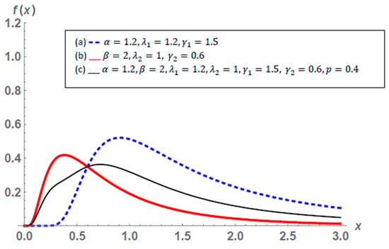
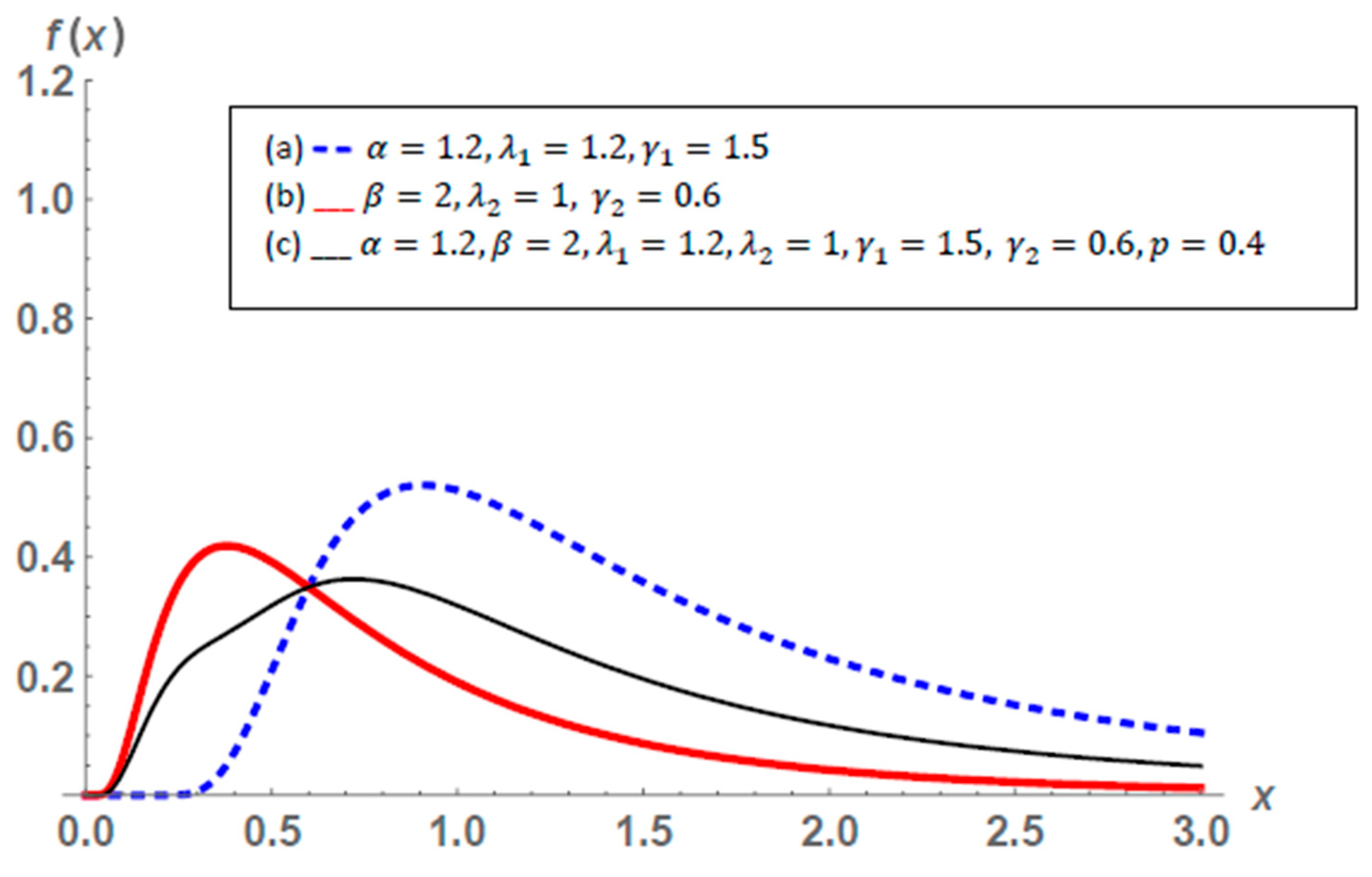
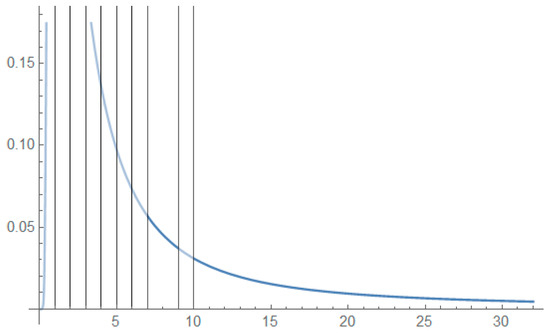
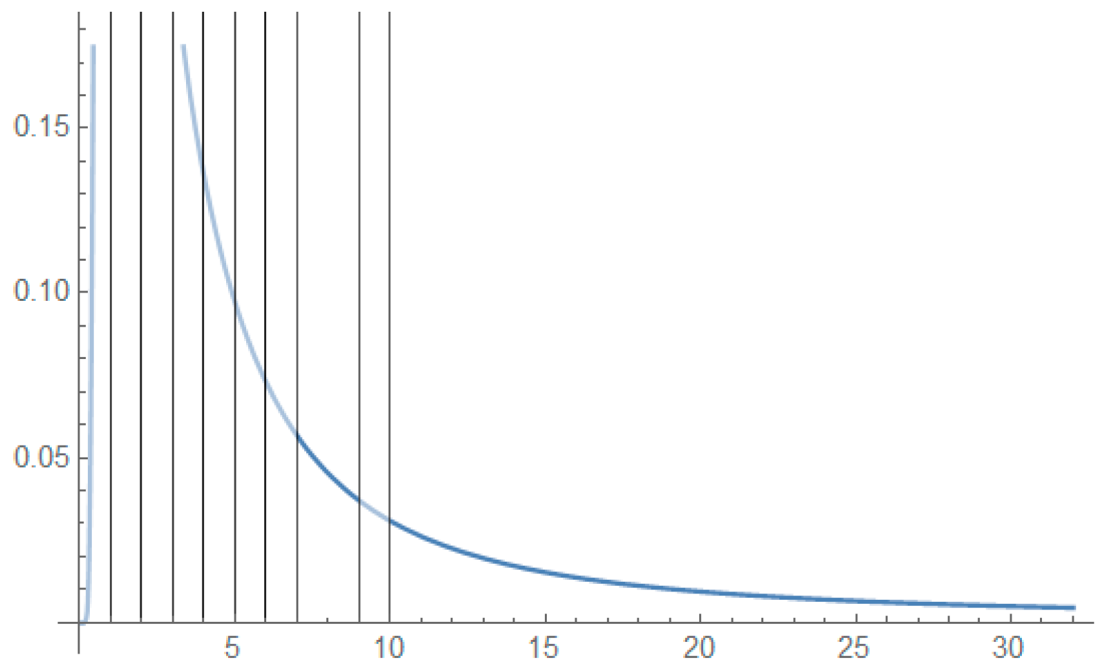
Figure 1 shows the pdf of the first component ($\alpha$, ${\lambda }_1$,${\gamma }_1$) in (a), the second component ($\beta$,${\lambda }_2$, ${\gamma }_2$) in (b) and the mixture of the two components, MENTL-IW, with parameters ($\alpha$,$\beta , {\lambda }_1$,${\lambda }_2$,${\gamma }_1,{\gamma }_2, p$) in (c).

Figure 1. Plots of the MENTL-IW distribution and its two component distributions.

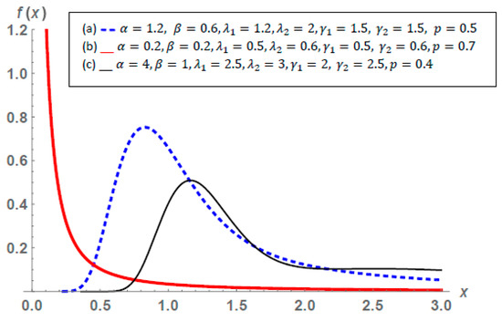
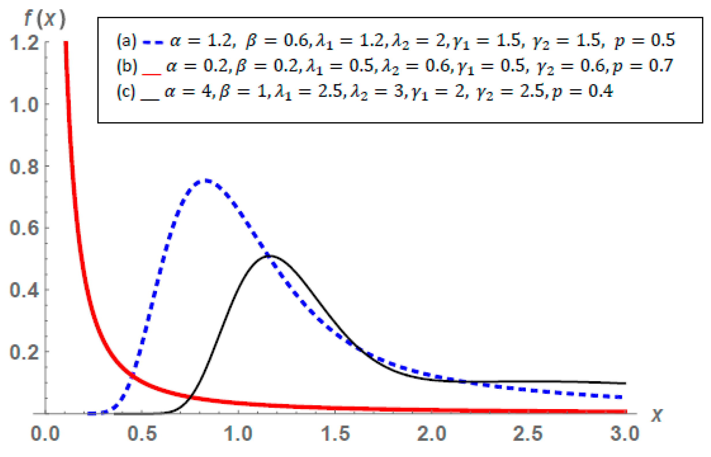
Figure 2 exhibits different shapes of the pdf for MENTL-IW distribution. The densities in (a) and (c) are unimodal and right-skewed. However, the density in (b) is decreasing.

Figure 2. Plots of the MENTL-IW pdf at different values of the parameters.

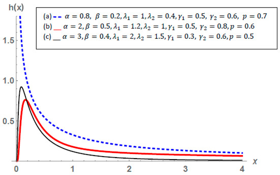
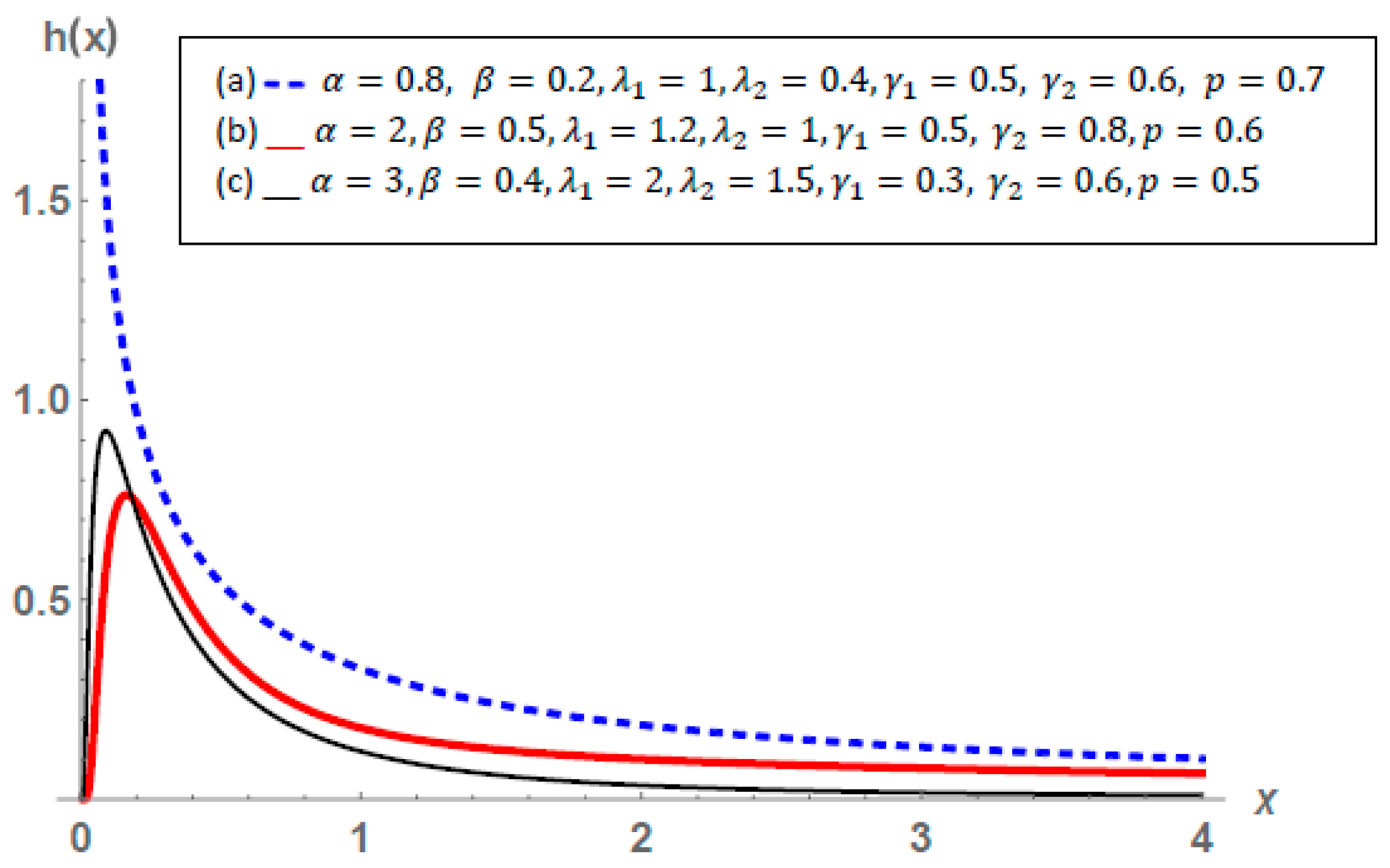
Figure 3 shows different shapes of the hrf for MENTL-IW distribution. The hrf in (a) is decreasing. The hrf in (b) and (c) are unimodal and right-skewed.

Figure 3. Plots of the MENTL-IW hrf for different parameter values.

3.2. Some Statistical Properties

3.2.1. Quantile Function

The quantile function of the MENTL-IW distribution can be derived as follows

using $G_1\left(x\right)=e^{-{\lambda }_1{x}^{-{\gamma }_1}}$, $H\left(x\right)={\displaystyle \frac{G_2\left(x\right)}{1-G_2\left(x\right)}}$ and $G_2\left(x\right)=e^{-{\lambda }_2{x}^{-{\gamma }_2}}$ into (12).

Also, $H\left(x\right)$ can be rewritten as $H\left(x\right)=-{(1-e^{{\lambda }_2{x}^{-{\gamma }_2}})}^{-1}$, then solve the following equation numerically

$$\mathit{ln}\left\{p{e}^{-{\lambda }_1\alpha {x_u}^{-{\gamma }_1}}+\left(1-p\right){\left[1-e^{2{(1-e^{{\lambda }_2{x_u}^{-{\gamma }_2}})}^{-1}}\right]}^{\beta }\right\}-\mathit{ln}u=0.$$

(24)

Subsequently, the random sample from the MENTL-IW distribution can be generated using the uniform distribution in (24).

3.2.2. Moments

The $r\mathrm{t}\mathrm{h}$ moment of the MENTL-IW distribution can be obtained by substituting $g_i\left(x\right)={{\lambda }_i{\gamma }_i{x}^{-{(\gamma }_i+1)}e}^{-{\lambda }_i{x}^{-{\gamma }_i}}$, $G_i\left(x\right)=e^{-{\lambda }_i{x}^{-{\gamma }_i}}$, $i=\mathrm{1,2}$ and $H\left(x\right)={\displaystyle \frac{G_2\left(x\right)}{1-G_2\left(x\right)}}$ in (13). Then, the $r\mathrm{t}\mathrm{h}$ moment about the origin of a random variable $X$ having the MENTL-IW distribution with the unknown parameters $(p,\alpha ,\beta ,{\lambda }_i \mathrm{a}\mathrm{n}\mathrm{d} {\gamma }_i)$ is obtained as given below.

$$\begin{gathered} {\mu }_r^{\prime }=\sum _{j_1=0}^{\infty }{\displaystyle \frac{{\left(\alpha -1\right)}^{j_1}}{j_1!}}{\left(-1\right)}^{j_1}{{\lambda }_1}^{\left(j_1+1\right)}{\gamma }_{1}p\alpha {\int }_0^{\infty }{x}^{\left(r-1\right)-{\gamma }_1\left(j_1+1\right)}{e}^{-{\lambda }_1{x}^{-{\gamma }_1}}dx \\ +\sum _{j_2=0}^{\infty } \sum _{j_3=0}^{\infty }{\left(-1\right)}^{j_2}{\left(-2\right)}^{j_3}\left({\displaystyle \genfrac{}{}{0pt}{}{\beta -1}{j_2}}\right){\displaystyle \frac{{\left(1+j_2\right)}^{j_3}}{j_3!}}2\left(1-p\right)\beta {\lambda }_2{\gamma }_2 \\ \times {\int }_0^{\infty }{x}^{r-\left({\gamma }_2+1\right)}{\displaystyle \frac{e^{-\left(1+j_3\right){\lambda }_2{x}^{-{\gamma }_2}}}{{\left(1-e^{-{\lambda }_2{x}^{-{\gamma }_2}}\right)}^{\left(2+j_3\right)}}}dx. \end{gathered}$$

(25)

Thus, the moments can be obtained by solving (25) numerically.

3.2.3. Moment-Generating Function

The moment-generating function of the MENTL-IW distribution can be found by replacing ${\mu }_r^{\prime }$ in (25) into (14), then

$$M_{x\left(M\right)}\left(t\right)=\sum _{r=0}^{\infty }{\displaystyle \frac{t^r}{r!}}\left[\begin{array}{c}{\displaystyle \sum _{j_1=0}^{\infty }}{\displaystyle \frac{{\left(\alpha -1\right)}^{j_1}}{j_1!}}{\left(-1\right)}^{j_1}{{\lambda }_1}^{\left(j_1+1\right)}{\gamma }_{1}p\alpha {\int }_0^{\infty }{x}^{\left(r-1\right)-{\gamma }_1\left(j_1+1\right)}{e}^{-{\lambda }_1{x}^{-{\gamma }_1}}dx\\ +{\displaystyle \sum _{j_2=0}^{\infty }} {\displaystyle \sum _{j_3=0}^{\infty }}{\left(-1\right)}^{j_2}{\left(-2\right)}^{j_3}\left({\displaystyle \genfrac{}{}{0pt}{}{\beta -1}{j_2}}\right){\displaystyle \frac{{\left(1+j_2\right)}^{j_3}}{j_3!}}2\left(1-p\right)\beta {\lambda }_2{\gamma }_2\\ \times {\int }_0^{\infty }{x}^{r-\left({\gamma }_2+1\right)}{\displaystyle \frac{e^{-\left(1+j_3\right){\lambda }_2{x}^{-{\gamma }_2}}}{{\left(1-e^{-{\lambda }_2{x}^{-{\gamma }_2}}\right)}^{\left(2+j_3\right)}}}dx\end{array}\right].$$

(26)

3.2.4. Distribution of Order Statistics

The $i\mathrm{t}\mathrm{h}$ order statistics for the MENTL-IW distribution can be obtained by substituting $g_i\left(x\right)={{\lambda }_i{\gamma }_i{x}^{-{(\gamma }_i+1)}e}^{-{\lambda }_i{x}^{-{\gamma }_i}}$, $G_i\left(x\right)=e^{-{\lambda }_i{x}^{-{\gamma }_i}}$, $i=\mathrm{1,2}$ and $H\left(x\right)={\displaystyle \frac{G_2\left(x\right)}{1-G_2\left(x\right)}}$ into (16); then,

$$\begin{array}{ll}{f}_{i,n}\left(x\right)& ={\displaystyle \sum _{k=0}^{n-i}}{\displaystyle \frac{n!{\left(-1\right)}^k}{\left(i-1\right)!k!\left(n-i-k\right)!}}\\ & \times \left(\begin{array}{c}p\alpha {{\lambda }_1{\gamma }_1{x}^{-{(\gamma }_1+1)}e}^{-{\alpha \lambda }_1{x}^{-{\gamma }_1}}\\ +{\displaystyle \frac{2\left(1-p\right)\beta {\lambda }_2{\gamma }_2{x}^{-{(\gamma }_2+1)}}{{\left[1-e^{-{\lambda }_2{x}^{-{\gamma }_2}}\right]}^2}}{e}^{-{\lambda }_2{x}^{-{\gamma }_2}+2{\left(1-e^{{\lambda }_2{x}^{-{\gamma }_2}}\right)}^{-1}}{\left[1-e^{2{\left(1-e^{{\lambda }_2{x}^{-{\gamma }_2}}\right)}^{-1}}\right]}^{\beta -1}\end{array}\right)\\ & \times {\left(p{e}^{-\alpha {\lambda }_1{x}^{-{\gamma }_1}}+\left(1-p\right){\left[1-e^{2{\left(1-e^{{\lambda }_2{x}^{-{\gamma }_2}}\right)}^{-1}}\right]}^{\beta }\right)}^{\left(i+k-1\right)}. \end{array}$$

(27)

Then, the corresponding smallest and largest order statistics of the MENTL-IW distribution can be obtained as a special case when $i=1, n$ in (27).

4. Estimation for Mixture of Two Exponentiated New Topp–Leone Inverse Weibull Distributions

This section introduces the ML estimation and Bayesian method for the unknown parameters, rf and hrf, of the MENTL-IW distribution.

4.1. Maximum Likelihood Estimation

This subsection focuses on deriving the ML estimators for the parameter vector $\underset{\_}{\mathsf{\Theta }}=\left(p, \alpha ,\beta ,{\lambda }_i,{\gamma }_i\right)$, rf and hrf of the MENTL-IW distribution based on a random sample of size n, where $i=\mathrm{1,2}$.

The likelihood function corresponding to the MENTL-IW density in (19) is given by

$$L_M\left(\underset{\_}{\theta };\underset{\_}{x}\right)=\prod _{j=1}^n\left[\begin{array}{c}p\alpha {\lambda }_1{\gamma }_1{x}^{-\left({\gamma }_1+1\right)}{e}^{-{\lambda }_1\alpha x^{-{\gamma }_1}}\\ +2\beta {\lambda }_2{\gamma }_2\left(1-p\right)x^{-\left({\gamma }_2+1\right)}{e}^{-{\lambda }_2{x}^{-{\gamma }_2}+2{\left(1-e^{{\lambda }_2{x}^{-{\gamma }_2}}\right)}^{-1}}{\displaystyle \frac{{\left[1-e^{2{\left(1-e^{{\lambda }_2{x}^{-{\gamma }_2}}\right)}^{-1}}\right]}^{\beta -1}}{{\left(1-e^{-{\lambda }_2{x}^{-{\gamma }_2}}\right)}^2}}\end{array}\right].$$

(28)

The natural logarithm of the likelihood function ${\mathcal{l}}_M\equiv lnL\left(\underset{\_}{\theta }; \underset{\_}{x}\right)$ is given by

$${\mathcal{l}}_M=\sum _{j=1}^{n}ln\left[\begin{array}{c}p\alpha {\lambda }_1{\gamma }_1{x}^{-\left({\gamma }_1+1\right)}{e}^{-{\lambda }_1\alpha x^{-{\gamma }_1}}\\ +2\beta {\lambda }_2{\gamma }_2\left(1-p\right)x^{-\left({\gamma }_2+1\right)}{e}^{-{\lambda }_2{x}^{-{\gamma }_2}+2{\left(1-e^{{\lambda }_2{x}^{-{\gamma }_2}}\right)}^{-1}}{\displaystyle \frac{{\left[1-e^{2{\left(1-e^{{\lambda }_2{x}^{-{\gamma }_2}}\right)}^{-1}}\right]}^{\beta -1}}{{\left(1-e^{-{\lambda }_2{x}^{-{\gamma }_2}}\right)}^2}}\end{array}\right].$$

(29)

By differentiating ${\mathcal{l}}_M$ with respect to the unknown parameters $\left(p, \alpha ,\beta ,{\lambda }_i,{\gamma }_i\right)$ of the MENTL-IW distribution, the first derivatives are obtained as follows:

$$\begin{array}{c}{\displaystyle \frac{\partial {\mathcal{l}}_M}{\partial p}}={\displaystyle \sum _{j=1}^n}{\displaystyle \frac{f_1\left(x_j,\widehat{\underset{\_}{\theta }}\right)-f_2\left(x_j,\widehat{\underset{\_}{\theta }}\right)}{f_M\left(x_j,\widehat{\underset{\_}{\theta }}\right)}}=0,\\ {\displaystyle \frac{\partial {\mathcal{l}}_M}{\partial \alpha }}={\displaystyle \sum _{j=1}^n}{\displaystyle \frac{\widehat{p}{\widehat{\lambda }}_1{\widehat{\gamma }}_1{x}^{-\left({\widehat{\gamma }}_1+1\right)}{e}^{-{\widehat{\lambda }}_1\widehat{\alpha }{x}^{-{\widehat{\gamma }}_1}}\left(1-{\widehat{\lambda }}_1\widehat{\alpha }{x}^{-{\widehat{\gamma }}_1}\right)}{f_M\left(x_j,\widehat{\underset{\_}{\theta }}\right)}}=0,\\ {\displaystyle \frac{\partial {\mathcal{l}}_M}{\partial \beta }}={\displaystyle \sum _{j=1}^n}{\displaystyle \frac{\phi \left(x_j,\widehat{\underset{\_}{\theta }}\right)}{f_M\left(x_j,\widehat{\underset{\_}{\theta }}\right)}}=0,\\ {\displaystyle \frac{\partial {\mathcal{l}}_M}{\partial {\lambda }_1}}={\displaystyle \sum _{j=1}^n}{\displaystyle \frac{\widehat{p}\widehat{\alpha }{\widehat{\gamma }}_1{x}^{-\left({\widehat{\gamma }}_1+1\right)}{e}^{-{\widehat{\lambda }}_1{x}^{-{\widehat{\gamma }}_1}}\left(1-{\widehat{\lambda }}_1{x}^{-{\widehat{\gamma }}_1}\right)}{f_M\left(x_j,\widehat{\underset{\_}{\theta }}\right)}}=0,\\ {\displaystyle \frac{\partial {\mathcal{l}}_M}{\partial {\gamma }_1}}={\displaystyle \sum _{j=1}^n}{\displaystyle \frac{\widehat{p}\widehat{\alpha }{{\widehat{\lambda }}_{1}x}^{-\left({\widehat{\gamma }}_1+1\right)}{e}^{-{\widehat{\lambda }}_1{x}^{-{\widehat{\gamma }}_1}+ln{\gamma }_1}\left[\mathrm{l}\mathrm{n}\left(x\right)({\widehat{\lambda }}_1{x}^{-{\widehat{\gamma }}_1}-1)+\frac{1}{{\gamma }_1}\right]}{f_M\left(x_j,\widehat{\underset{\_}{\theta }}\right)}}=0, \\ \mathrm{and}\\ {\displaystyle \frac{\partial {\mathcal{l}}_M}{\partial {\gamma }_2}}={\displaystyle \sum _{j=1}^n}\left[2\widehat{\beta }{\widehat{\lambda }}_2\left(1-\widehat{p}\right){\displaystyle \frac{\left[{\tau }_1\left(x_j,\widehat{\underset{\_}{\theta }}\right)\times {\tau }_2\left(x_j,\widehat{\underset{\_}{\theta }}\right)\right]+\left[{\omega }_1\left(x_j,\widehat{\underset{\_}{\theta }}\right)\times {\tau }_3\left(x_j,\widehat{\underset{\_}{\theta }}\right)\right]}{f_M\left(x_j,\widehat{\underset{\_}{\theta }}\right)}}\right]=0,\end{array}$$

(30)

where $f_1\left(x_j,\underset{\_}{\theta }\right)$, $f_2\left(x_j,\underset{\_}{\theta }\right)$, $\phi \left(x_j,\underset{\_}{\theta }\right)$, ${\omega }_1\left(x_j,\underset{\_}{\theta }\right)$, ${\omega }_2\left(x_j,\underset{\_}{\theta }\right)$, ${\omega }_3\left(x_j,\underset{\_}{\theta }\right),{\omega }_4\left(x_j,\underset{\_}{\theta }\right)$, ${\tau }_1\left(x_j,\widehat{\underset{\_}{\theta }}\right)$, ${\tau }_2\left(x_j,\widehat{\underset{\_}{\theta }}\right)$, ${\tau }_3\left(x_j,\underset{\_}{\theta }\right)$ and $f_M\left(x_j,\widehat{\underset{\_}{\theta }}\right)$ are

$$\begin{array}{cc}{ f}_1\left(x_j,\underset{\_}{\theta }\right)& =\widehat{\alpha }{\widehat{\lambda }}_1{\widehat{\gamma }}_1{x}^{-\left({\widehat{\gamma }}_1+1\right)}{e}^{-\widehat{\alpha }{\widehat{\lambda }}_1{x}^{-{\widehat{\gamma }}_1}},\\ f_2\left(x_j,\underset{\_}{\theta }\right)& =2\widehat{\beta }{\widehat{\lambda }}_2{\widehat{\gamma }}_2{x}^{-\left({\widehat{\gamma }}_2+1\right)}{e}^{-{\widehat{\lambda }}_2{x}^{-{\widehat{\gamma }}_2}+2{\left(1-e^{{\widehat{\lambda }}_2{x}^{-{\widehat{\gamma }}_2}}\right)}^{-1}}{\omega }_2\left(x_j,\underset{\_}{\theta }\right),\\ \phi \left(x_j,\underset{\_}{\theta }\right)& =2{\widehat{\lambda }}_2{\widehat{\gamma }}_2\left(1-\widehat{p}\right)x^{-\left({\widehat{\gamma }}_2+1\right)}{e}^{-{\widehat{\lambda }}_2{x}^{-{\widehat{\gamma }}_2}+2{\left(1-e^{{\widehat{\lambda }}_2{x}^{-{\widehat{\gamma }}_2}}\right)}^{-1}}{\omega }_2\left(x_j,\underset{\_}{\theta }\right)\\ & \times \left[\widehat{\beta }ln\left(1-e^{2{\left(1-e^{{\widehat{\lambda }}_2{x}^{-{\widehat{\gamma }}_2}}\right)}^{-1}}\right)+1\right],\\ {\omega }_1\left(x_j,\underset{\_}{\theta }\right)& =e^{ln{\widehat{\lambda }}_2-{\widehat{\lambda }}_2{x}^{-{\widehat{\gamma }}_2}+2{\left(1-e^{{\widehat{\lambda }}_2{x}^{-{\widehat{\gamma }}_2}}\right)}^{-1}},\\ {\omega }_2\left(x_j,\underset{\_}{\theta }\right)& ={\displaystyle \frac{{\left[1-e^{2{\left(1-e^{{\widehat{\lambda }}_2{x}^{-{\widehat{\gamma }}_2}}\right)}^{-1}}\right]}^{\widehat{\beta }-1}}{{\left(1-e^{-{\widehat{\lambda }}_2{x}^{-{\widehat{\gamma }}_2}}\right)}^2}},\\ {\omega }_3\left(x_j,\underset{\_}{\theta }\right)& ={\displaystyle \frac{-2x^{-{\widehat{\gamma }}_2}{e}^{{\widehat{\lambda }}_2{x}^{-{\widehat{\gamma }}_2}}}{{\left(1-e^{-{\widehat{\lambda }}_2{x}^{-{\widehat{\gamma }}_2}}\right)}^4}}\\ & \times \{\left[\left(\widehat{\beta }-1\right)e^{2{\left(1-e^{{\widehat{\lambda }}_2{x}^{-{\widehat{\gamma }}_2}}\right)}^{-1}}{\left(1-e^{2{\left(1-e^{{\widehat{\lambda }}_2{x}^{-{\widehat{\gamma }}_2}}\right)}^{-1}}\right)}^{\widehat{\beta }-2}{\displaystyle \frac{{\left(1-e^{-{\widehat{\lambda }}_2{x}^{-{\widehat{\gamma }}_2}}\right)}^2}{{\left(1-e^{{\widehat{\lambda }}_2{x}^{-{\widehat{\gamma }}_2}}\right)}^2}}\right]\\ & +\left[{\left(1-e^{2{\left(1-e^{{\widehat{\lambda }}_2{x}^{-{\widehat{\gamma }}_2}}\right)}^{-1}}\right)}^{\widehat{\beta }-1}\left(1-e^{-{\widehat{\lambda }}_2{x}^{-{\widehat{\gamma }}_2}}\right)\right]\},\\ {\omega }_4\left(x_j,\underset{\_}{\theta }\right)& ={\omega }_1\left(x_j,\underset{\_}{\theta }\right)\left[{\displaystyle \frac{1}{{\widehat{\lambda }}_2}}-x^{-{\widehat{\gamma }}_2}+\left(2x^{-{\widehat{\gamma }}_2}{e}^{{\widehat{\lambda }}_2{x}^{-{\widehat{\gamma }}_2}}{\left(1-e^{{\widehat{\lambda }}_2{x}^{-{\widehat{\gamma }}_2}}\right)}^{-2}\right)\right],\\ {\tau }_1\left(x_j,\widehat{\underset{\_}{\theta }}\right)& =x^{-\left({\widehat{\gamma }}_2+1\right)}{\omega }_1\left(x_j,\underset{\_}{\theta }\right),\\ {\tau }_2\left(x_j,\widehat{\underset{\_}{\theta }}\right)& ={\displaystyle \frac{2{\widehat{\lambda }}_2{x}^{-{\widehat{\gamma }}_2}lnx}{{\left(1-e^{-{\widehat{\lambda }}_2{x}^{-{\widehat{\gamma }}_2}}\right)}^4}}\\ & \times \left\{\begin{array}{c}\left[e^{{-\widehat{\lambda }}_2{x}^{-{\widehat{\gamma }}_2}}\left(1-e^{-{\widehat{\lambda }}_2{x}^{-{\widehat{\gamma }}_2}}\right){\left(1-e^{2{\left(1-e^{{\widehat{\lambda }}_2{x}^{-{\widehat{\gamma }}_2}}\right)}^{-1}}\right)}^{\widehat{\beta }-1}\right]\\ +\left[\left(\widehat{\beta }-1\right)e^{{\widehat{\lambda }}_2{x}^{-{\widehat{\gamma }}_2}+2{\left(1-e^{{\widehat{\lambda }}_2{x}^{-{\widehat{\gamma }}_2}}\right)}^{-1}}{\left(1-e^{2{\left(1-e^{{\widehat{\lambda }}_2{x}^{-{\widehat{\gamma }}_2}}\right)}^{-1}}\right)}^{\widehat{\beta }-2}{\displaystyle \frac{{\left(1-e^{-{\widehat{\lambda }}_2{x}^{-{\widehat{\gamma }}_2}}\right)}^2}{{\left(1-e^{{\widehat{\lambda }}_2{x}^{-{\widehat{\gamma }}_2}}\right)}^2}}\right]\end{array}\right\},\\ & {\tau }_3\left(x_j,\underset{\_}{\theta }\right)={\tau }_1\left(x_j,\widehat{\underset{\_}{\theta }}\right)\times \left[{\displaystyle \frac{1}{{\widehat{\gamma }}_2}}-2{\widehat{\lambda }}_2{x}^{-{\widehat{\gamma }}_2}lnx{\left(1-e^{{\widehat{\lambda }}_2{x}^{-{\widehat{\gamma }}_2}}\right)}^{-2}\right],\end{array}$$

and $f_M\left(x_j,\widehat{\underset{\_}{\theta }}\right)$ is the pdf of the MENTL-IW distribution in (19).

Solving (30) numerically, one can obtain the ML estimates of the unknown parameters.

ML estimation was employed to estimate the unknown model parameters. The Newton–Raphson method, an iterative optimization algorithm, was used to find the parameter values that maximize the likelihood function. This involves iteratively calculating the gradient and Hessian matrix of the log-likelihood function. Convergence criteria, such as the magnitude of the gradient or the change in parameter values between iterations, were monitored to ensure the algorithm converged to a stable solution.

The ML estimators of the rf and hrf can be obtained by replacing the parameters $\left(p, \alpha ,\beta ,{\lambda }_1,{\lambda }_2,{\gamma }_1 \mathrm{a}\mathrm{n}\mathrm{d} {\gamma }_2\right)$ in (21) and (22) by their corresponding ML estimators. Then, the ML estimators of $S_M\left(x\right)$ and $h_M\left(x\right)$ are given by

$${\widehat{S}}_M\left(x\right)=1-\widehat{p}{e}^{-{\widehat{\lambda }}_1\widehat{\alpha }{x}^{-{\widehat{\gamma }}_1}}-\left(1-\widehat{p}\right){\left[1-e^{2{\left(1-e^{{\widehat{\lambda }}_2{x}^{-{\widehat{\gamma }}_2}}\right)}^{-1}}\right]}^{\widehat{\beta }}$$

(31)

and

$${\widehat{h}}_M\left(x\right)={\displaystyle \frac{\widehat{p}\widehat{\alpha }{\widehat{\lambda }}_1{\widehat{\gamma }}_1{x}^{-\left({\widehat{\gamma }}_1+1\right)}{e}^{-{\widehat{\lambda }}_1\widehat{\alpha }{x}^{-{\widehat{\gamma }}_1}}+2\widehat{\beta }{\widehat{\lambda }}_2{\widehat{\gamma }}_2\left(1-\widehat{p}\right)x^{-\left({\widehat{\gamma }}_2+1\right)}{e}^{-{\widehat{\lambda }}_2{x}^{-{\widehat{\gamma }}_2}+2{\left(1-e^{{\widehat{\lambda }}_2{x}^{-{\widehat{\gamma }}_2}}\right)}^{-1}}\frac{{\left[1-e^{2{\left(1-e^{{\widehat{\lambda }}_2{x}^{-{\widehat{\gamma }}_2}}\right)}^{-1}}\right]}^{\widehat{\beta }-1}}{{\left(1-e^{-{\widehat{\lambda }}_2{x}^{-{\widehat{\gamma }}_2}}\right)}^2}}{1-\widehat{p}{e}^{-{\widehat{\lambda }}_1\widehat{\alpha }{x}^{-{\widehat{\gamma }}_1}}-\left(1-\widehat{p}\right){\left[1-e^{2{\left(1-e^{{\widehat{\lambda }}_2{x}^{-{\widehat{\gamma }}_2}}\right)}^{-1}}\right]}^{\widehat{\beta }}}}$$

(32)

4.2. Bayesian Estimation

In this subsection, the Bayes estimators of the unknown parameters of the MENTL-IW distribution are obtained using the conjugate prior under the SE and LINEX loss functions, assuming that the unknown parameters $\underset{\_}{\theta }=\left(p,\alpha ,\beta ,{\lambda }_1,{\lambda }_2,{\gamma }_1,{\gamma }_2\right)=({\theta }_1,{\theta }_2,{\theta }_3,{\theta }_4,{\theta }_5,{\theta }_6,{\theta }_7)$ are independent random variables with beta prior distribution, which is assumed for $\left({\theta }_1=p\right)$ and gamma prior distribution, where $\left(\alpha ,\beta ,{\lambda }_1,{\lambda }_2,{\gamma }_1,{\gamma }_2\right)=({\theta }_2,{\theta }_3,{\theta }_4,{\theta }_5,{\theta }_6,{\theta }_7)$. Then, the joint prior density function for the vector of $\underset{\_}{\theta }$ is given by

$$\begin{array}{ll}\pi \left(\underset{\_}{\theta }\right)& ={\pi }_1\left(p\right){\pi }_2\left(\alpha \right){\pi }_3\left(\beta \right){\pi }_4\left({\lambda }_1\right){\pi }_5\left({\lambda }_2\right){\pi }_6\left({\gamma }_1\right){\pi }_7\left({\gamma }_2\right)\\ & ={\displaystyle \frac{1}{\mathrm{B}\left(a_1,a_2\right)}} p^{a_1-1}{\left(1-p\right)}^{a_2-1}\\ & \times {\displaystyle \frac{{b_2}^{b_1}{b_4}^{b_3}{b_6}^{b_5}{b_8}^{b_7}{b_{10}}^{b_9}{b_{12}}^{b_{11}}}{\mathsf{\Gamma }{b}_1\mathsf{\Gamma }{b}_3\mathsf{\Gamma }{b}_5\mathsf{\Gamma }{b}_7\mathsf{\Gamma }{b}_9\mathsf{\Gamma }{b}_{11}}}{\alpha }^{b_1-1}{\beta }^{b_3-1}{{\lambda }_1}^{b_5-1}{{\lambda }_2}^{b_7-1}{{\gamma }_1}^{b_9-1}{{\gamma }_2}^{b_{11}-1}\\ & \times e^{-\left(\alpha b_2+\beta b_4+{\lambda }_1{b}_6+{\lambda }_2{b}_8+{\gamma }_1{b}_{10}+{\gamma }_2{b}_{12}\right)},\end{array}$$

(33)

where $a_i=a_1,a_2$ and $b_j=b_1,b_2,\dots ,b_{12}$ are the hyper parameters of the prior distribution,

$$0<p<1, \alpha ,\beta ,{\lambda }_1,{\lambda }_2,{\gamma }_1,{\gamma }_2,a_i,b_j>0$$

Using (28) and (33), then the joint posterior density function of $\underset{\_}{\theta }$ can be derived as given below

$$\begin{array}{ll}\pi \left(\underset{\_}{\theta }|\underset{\_}{x}\right)& =k\times \pi \left(\underset{\_}{\theta }\right)\\ & \times {\displaystyle \prod _{j=1}^n}\left[\begin{array}{c}p\alpha {\lambda }_1{\gamma }_1{x}^{-\left({\gamma }_1+1\right)}{e}^{-{\lambda }_1\alpha x^{-{\gamma }_1}}\\ +2\beta {\lambda }_2{\gamma }_2(1-p)x^{-\left({\gamma }_2+1\right)}{e}^{-{\lambda }_2{x}^{-{\gamma }_2}+2{\left(1-e^{{\lambda }_2{x}^{-{\gamma }_2}}\right)}^{-1}}{\displaystyle \frac{{\left[1-e^{2{\left(1-e^{{\lambda }_2{x}^{-{\gamma }_2}}\right)}^{-1}}\right]}^{\beta -1}}{{\left(1-e^{-{\lambda }_2{x}^{-{\gamma }_2}}\right)}^2}}\end{array}\right]\end{array}$$

(34)

where

$$\begin{array}{ll}{k}^{-1}& ={\int }_{\underset{\_}{\theta }}\pi \left(\underset{\_}{\theta }\right)L\left(\underset{\_}{\theta }\left|\underset{\_}{x}\right.\right)d\underset{\_}{\theta }\\ & ={\int }_{\underset{\_}{\theta }}\pi \left(\underset{\_}{\theta }\right)\times {\displaystyle \prod _{j=1}^n}\left[\begin{array}{c}p\alpha {\lambda }_1{\gamma }_1{x}^{-\left({\gamma }_1+1\right)}{e}^{-{\lambda }_1\alpha x^{-{\gamma }_1}}\\ +2\beta {\lambda }_2{\gamma }_2(1-p)x^{-\left({\gamma }_2+1\right)}{e}^{-{\lambda }_2{x}^{-{\gamma }_2}+2{\left(1-e^{{\lambda }_2{x}^{-{\gamma }_2}}\right)}^{-1}}{\displaystyle \frac{{\left[1-e^{2{\left(1-e^{{\lambda }_2{x}^{-{\gamma }_2}}\right)}^{-1}}\right]}^{\beta -1}}{{\left(1-e^{-{\lambda }_2{x}^{-{\gamma }_2}}\right)}^2}}\end{array}\right]d\underset{\_}{\theta }, \end{array}$$

and

$${\int }_{\underset{\_}{\theta }} ={\int }_0^1 {\int }_0^{\infty } {\int }_0^{\infty } {\int }_0^{\infty } {\int }_0^{\infty } {\int }_0^{\infty } {\int }_0^{\infty } \mathrm{and} d\underset{\_}{\theta }=dpd\alpha d\beta d{\lambda }_{1}d{\lambda }_{2}d{\gamma }_{1}d{\gamma }_2.$$

Thus, the marginal posterior distribution of each parameter can be obtained by integrating the joint posterior distribution (34) with respect to other parameters as follows:

$$\begin{array}{ll}\pi \left(p|\underset{\_}{x}\right)& =k{\int }_0^{\infty } {\int }_0^{\infty } {\int }_0^{\infty } {\int }_0^{\infty } {\int }_0^{\infty } {\int }_0^{\infty } \pi \left(\underset{\_}{\theta }\right)\\ & \times {\displaystyle \prod _{j=1}^n}\left[\begin{array}{c}p\alpha {\lambda }_1{\gamma }_1{x}^{-\left({\gamma }_1+1\right)}{e}^{-{\lambda }_1\alpha x^{-{\gamma }_1}}\\ +2\beta {\lambda }_2{\gamma }_2\left(1-p\right)x^{-\left({\gamma }_2+1\right)}{e}^{-{\lambda }_2{x}^{-{\gamma }_2}+2{\left(1-e^{{\lambda }_2{x}^{-{\gamma }_2}}\right)}^{-1}}{\displaystyle \frac{{\left[1-e^{2{\left(1-e^{{\lambda }_2{x}^{-{\gamma }_2}}\right)}^{-1}}\right]}^{\beta -1}}{{\left(1-e^{-{\lambda }_2{x}^{-{\gamma }_2}}\right)}^2}}\end{array}\right]d\alpha d\beta d{\lambda }_{1}d{\lambda }_{2}d{\gamma }_{1}d{\gamma }_2,\\ & 0<p<1, \end{array}$$

(35)

$$\begin{array}{cc}\pi \left(\alpha |\underset{\_}{x}\right)& =k{\int }_0^{\infty } {\int }_0^{\infty } {\int }_0^{\infty } {\int }_0^{\infty } {\int }_0^{\infty } {\int }_0^1 \pi \left(\underset{\_}{\theta }\right)\\ & \times {\displaystyle \prod _{j=1}^n}\left[\begin{array}{c}p\alpha {\lambda }_1{\gamma }_1{x}^{-\left({\gamma }_1+1\right)}{e}^{-{\lambda }_1\alpha x^{-{\gamma }_1}}\\ +2\beta {\lambda }_2{\gamma }_2\left(1-p\right)x^{-\left({\gamma }_2+1\right)}{e}^{-{\lambda }_2{x}^{-{\gamma }_2}+2{\left(1-e^{{\lambda }_2{x}^{-{\gamma }_2}}\right)}^{-1}}{\displaystyle \frac{{\left[1-e^{2{\left(1-e^{{\lambda }_2{x}^{-{\gamma }_2}}\right)}^{-1}}\right]}^{\beta -1}}{{\left(1-e^{-{\lambda }_2{x}^{-{\gamma }_2}}\right)}^2}}\end{array}\right]dpd\beta d{\lambda }_{1}d{\lambda }_{2}d{\gamma }_{1}d{\gamma }_2,\\ & \alpha >0, \end{array}$$

(36)

$$\begin{array}{cc}\pi \left(\beta |\underset{\_}{x}\right)& =k{\int }_0^{\infty } {\int }_0^{\infty } {\int }_0^{\infty } {\int }_0^{\infty } {\int }_0^{\infty } {\int }_0^1 \pi \left(\underset{\_}{\theta }\right)\\ & \times {\displaystyle \prod _{j=1}^n}\left[\begin{array}{c}p\alpha {\lambda }_1{\gamma }_1{x}^{-\left({\gamma }_1+1\right)}{e}^{-{\lambda }_1\alpha x^{-{\gamma }_1}}\\ +2\beta {\lambda }_2{\gamma }_2\left(1-p\right)x^{-\left({\gamma }_2+1\right)}{e}^{-{\lambda }_2{x}^{-{\gamma }_2}+2{\left(1-e^{{\lambda }_2{x}^{-{\gamma }_2}}\right)}^{-1}}{\displaystyle \frac{{\left[1-e^{2{\left(1-e^{{\lambda }_2{x}^{-{\gamma }_2}}\right)}^{-1}}\right]}^{\beta -1}}{{\left(1-e^{-{\lambda }_2{x}^{-{\gamma }_2}}\right)}^2}}\end{array}\right]dpd\alpha d{\lambda }_{1}d{\lambda }_{2}d{\gamma }_{1}d{\gamma }_2,\\ & \beta >0,\end{array}$$

(37)

$$\begin{array}{cc}\pi \left({\lambda }_1|\underset{\_}{x}\right)& =k{\int }_0^{\infty } {\int }_0^{\infty } {\int }_0^{\infty } {\int }_0^{\infty } {\int }_0^{\infty } {\int }_0^1 \pi \left(\underset{\_}{\theta }\right)\\ & \times {\displaystyle \prod _{j=1}^n}\left[\begin{array}{c}p\alpha {\lambda }_1{\gamma }_1{x}^{-\left({\gamma }_1+1\right)}{e}^{-{\lambda }_1\alpha x^{-{\gamma }_1}}\\ +2\beta {\lambda }_2{\gamma }_2\left(1-p\right)x^{-\left({\gamma }_2+1\right)}{e}^{-{\lambda }_2{x}^{-{\gamma }_2}+2{\left(1-e^{{\lambda }_2{x}^{-{\gamma }_2}}\right)}^{-1}}{\displaystyle \frac{{\left[1-e^{2{\left(1-e^{{\lambda }_2{x}^{-{\gamma }_2}}\right)}^{-1}}\right]}^{\beta -1}}{{\left(1-e^{-{\lambda }_2{x}^{-{\gamma }_2}}\right)}^2}}\end{array}\right]dpd\alpha d\beta d{\lambda }_{2}d{\gamma }_{1}d{\gamma }_2,\\ & {\lambda }_1>0, \end{array}$$

(38)

$$\begin{array}{cc}\pi \left({\lambda }_2|\underset{\_}{x}\right)& =k{\int }_0^{\infty } {\int }_0^{\infty } {\int }_0^{\infty } {\int }_0^{\infty } {\int }_0^{\infty } {\int }_0^1 \pi \left(\underset{\_}{\theta }\right)\\ & \times {\displaystyle \prod _{j=1}^n}\left[\begin{array}{c}p\alpha {\lambda }_1{\gamma }_1{x}^{-\left({\gamma }_1+1\right)}{e}^{-{\lambda }_1\alpha x^{-{\gamma }_1}}\\ +2\beta {\lambda }_2{\gamma }_2\left(1-p\right)x^{-\left({\gamma }_2+1\right)}{e}^{-{\lambda }_2{x}^{-{\gamma }_2}+2{\left(1-e^{{\lambda }_2{x}^{-{\gamma }_2}}\right)}^{-1}}{\displaystyle \frac{{\left[1-e^{2{\left(1-e^{{\lambda }_2{x}^{-{\gamma }_2}}\right)}^{-1}}\right]}^{\beta -1}}{{\left(1-e^{-{\lambda }_2{x}^{-{\gamma }_2}}\right)}^2}}\end{array}\right]dpd\alpha d\beta d{\lambda }_{1}d{\gamma }_{1}d{\gamma }_2,\\ & {\lambda }_2>0, \end{array}$$

(39)

$$\begin{array}{cc}\pi \left({\gamma }_1|\underset{\_}{x}\right)& =k{\int }_0^{\infty } {\int }_0^{\infty } {\int }_0^{\infty } {\int }_0^{\infty } {\int }_0^{\infty } {\int }_0^1 \pi \left(\underset{\_}{\theta }\right)\\ & \times {\displaystyle \prod _{j=1}^n}\left[\begin{array}{c}p\alpha {\lambda }_1{\gamma }_1{x}^{-\left({\gamma }_1+1\right)}{e}^{-{\lambda }_1\alpha x^{-{\gamma }_1}}\\ +2\beta {\lambda }_2{\gamma }_2\left(1-p\right)x^{-\left({\gamma }_2+1\right)}{e}^{-{\lambda }_2{x}^{-{\gamma }_2}+2{\left(1-e^{{\lambda }_2{x}^{-{\gamma }_2}}\right)}^{-1}}{\displaystyle \frac{{\left[1-e^{2{\left(1-e^{{\lambda }_2{x}^{-{\gamma }_2}}\right)}^{-1}}\right]}^{\beta -1}}{{\left(1-e^{-{\lambda }_2{x}^{-{\gamma }_2}}\right)}^2}}\end{array}\right]dpd\alpha d\beta d{\lambda }_{1}d{\lambda }_{2}d{\gamma }_2,\\ & {\gamma }_1>0, \end{array}$$

(40)

and

$$\begin{array}{cc}\pi \left({\gamma }_2|\underset{\_}{x}\right)& =k{\int }_0^{\infty } {\int }_0^{\infty } {\int }_0^{\infty } {\int }_0^{\infty } {\int }_0^{\infty } {\int }_0^1 \pi \left(\underset{\_}{\theta }\right)\\ & \times {\displaystyle \prod _{j=1}^n}\left[\begin{array}{c}p\alpha {\lambda }_1{\gamma }_1{x}^{-\left({\gamma }_1+1\right)}{e}^{-{\lambda }_1\alpha x^{-{\gamma }_1}}\\ +2\beta {\lambda }_2{\gamma }_2\left(1-p\right)x^{-\left({\gamma }_2+1\right)}{e}^{-{\lambda }_2{x}^{-{\gamma }_2}+2{\left(1-e^{{\lambda }_2{x}^{-{\gamma }_2}}\right)}^{-1}}{\displaystyle \frac{{\left[1-e^{2{\left(1-e^{{\lambda }_2{x}^{-{\gamma }_2}}\right)}^{-1}}\right]}^{\beta -1}}{{\left(1-e^{-{\lambda }_2{x}^{-{\gamma }_2}}\right)}^2}}\end{array}\right]dpd\alpha d\beta d{\lambda }_{1}d{\lambda }_{2}d{\gamma }_1,\\ & {\gamma }_2>0. \end{array}$$

(41)

Then, the posterior distributions (35)–(41) can be used to obtain the Bayes estimators for the parameters from the MENTL-IW distribution under the SE and LINEX loss functions.

• Bayesian estimation of mixture exponentiated new Topp–Leone inverse Weibull distribution under squared error loss function

Under the SE loss function, the Bayes estimators of the vector of parameters $\underset{\_}{\theta }$ is the mean of the posterior distribution, which can be derived from their marginal posterior distributions as follows:

$${\theta }_{j\left(SE\right)}^{\star }=E\left({\theta }_j| \underset{\_}{x}\right)={\int }_{{\theta }_j}{\theta }_j\pi \left(\underset{\_}{\theta }|\underset{\_}{x}\right)d{\theta }_j,j=\mathrm{1,2},\mathrm{3,4},\mathrm{5,6},7,$$

(42)

where ${\theta }_1=p,{\theta }_2=\alpha ,{\theta }_3=\beta ,{\theta }_4={\lambda }_1,{\theta }_5={\lambda }_2,{\theta }_6={\gamma }_1 \mathrm{a}\mathrm{n}\mathrm{d} {\theta }_7={\gamma }_2.$

Thus, the Bayes estimator of the proportion mixing $p$ is

$$\begin{array}{l}{p}_{\left(SE\right)}^{\star }=E\left(p| \underset{\_}{x}\right)={\int }_0^{1}p\pi \left(p|\underset{\_}{x}\right)dp\\ =k{\int }_0^1{\int }_0^{\infty } {\int }_0^{\infty } {\int }_0^{\infty } {\int }_0^{\infty } {\int }_0^{\infty } {\int }_0^{\infty }p \pi \left(\underset{\_}{\theta }\right)\\ \times {\displaystyle \prod _{j=1}^n}\left[\begin{array}{c}p\alpha {\lambda }_1{\gamma }_1{x}^{-\left({\gamma }_1+1\right)}{e}^{-{\lambda }_1\alpha x^{-{\gamma }_1}}\\ +2\beta {\lambda }_2{\gamma }_2\left(1-p\right)x^{-\left({\gamma }_2+1\right)}{e}^{-{\lambda }_2{x}^{-{\gamma }_2}+2{\left(1-e^{{\lambda }_2{x}^{-{\gamma }_2}}\right)}^{-1}}{\displaystyle \frac{{\left[1-e^{2{\left(1-e^{{\lambda }_2{x}^{-{\gamma }_2}}\right)}^{-1}}\right]}^{\beta -1}}{{\left(1-e^{-{\lambda }_2{x}^{-{\gamma }_2}}\right)}^2}}\end{array}\right]d\alpha d\beta d{\lambda }_{1}d{\lambda }_{2}d{\gamma }_{1}d{\gamma }_{2}dp.\end{array}$$

(43)

Similarly, the Bayes estimators of the parameters $\alpha ,\beta ,{\lambda }_1,{\lambda }_2,{\gamma }_1 \mathrm{a}\mathrm{n}\mathrm{d} {\gamma }_2$ are given by

$$\begin{array}{l}{\alpha }_{\left(SE\right)}^{\star }=E\left(\alpha | \underset{\_}{x}\right)={\int }_0^{\infty }\alpha \pi \left(\alpha |\underset{\_}{x}\right)d\alpha \\ =k{\int }_0^{\infty }{\int }_0^{\infty } {\int }_0^{\infty } {\int }_0^{\infty } {\int }_0^{\infty } {\int }_0^{\infty } {\int }_0^1\alpha \pi \left(\underset{\_}{\theta }\right)\\ \times {\displaystyle \prod _{j=1}^n}\left[\begin{array}{c}p\alpha {\lambda }_1{\gamma }_1{x}^{-\left({\gamma }_1+1\right)}{e}^{-{\lambda }_1\alpha x^{-{\gamma }_1}}\\ +2\beta {\lambda }_2{\gamma }_2\left(1-p\right)x^{-\left({\gamma }_2+1\right)}{e}^{-{\lambda }_2{x}^{-{\gamma }_2}+2{\left(1-e^{{\lambda }_2{x}^{-{\gamma }_2}}\right)}^{-1}}{\displaystyle \frac{{\left[1-e^{2{\left(1-e^{{\lambda }_2{x}^{-{\gamma }_2}}\right)}^{-1}}\right]}^{\beta -1}}{{\left(1-e^{-{\lambda }_2{x}^{-{\gamma }_2}}\right)}^2}}\end{array}\right]dpd\beta d{\lambda }_{1}d{\lambda }_{2}d{\gamma }_{1}d{\gamma }_{2}d\alpha ,\end{array}$$

(44)

$$\begin{array}{l}{\beta }_{\left(SE\right)}^{\star }=E\left(\beta | \underset{\_}{x}\right)={\int }_0^{\infty }\beta \pi \left(\beta |\underset{\_}{x}\right)d\beta \\ =k{\int }_0^{\infty }{\int }_0^{\infty } {\int }_0^{\infty } {\int }_0^{\infty } {\int }_0^{\infty } {\int }_0^{\infty } {\int }_0^1 \beta \pi \left(\underset{\_}{\theta }\right)\\ \times {\displaystyle \prod _{j=1}^n}\left[\begin{array}{c}p\alpha {\lambda }_1{\gamma }_1{x}^{-\left({\gamma }_1+1\right)}{e}^{-{\lambda }_1\alpha x^{-{\gamma }_1}}\\ +2\beta {\lambda }_2{\gamma }_2\left(1-p\right)x^{-\left({\gamma }_2+1\right)}{e}^{-{\lambda }_2{x}^{-{\gamma }_2}+2{\left(1-e^{{\lambda }_2{x}^{-{\gamma }_2}}\right)}^{-1}}{\displaystyle \frac{{\left[1-e^{2{\left(1-e^{{\lambda }_2{x}^{-{\gamma }_2}}\right)}^{-1}}\right]}^{\beta -1}}{{\left(1-e^{-{\lambda }_2{x}^{-{\gamma }_2}}\right)}^2}}\end{array}\right]dpd\alpha d{\lambda }_{1}d{\lambda }_{2}d{\gamma }_{1}d{\gamma }_{2}d\beta ,\end{array}$$

(45)

$$\begin{array}{l}{\lambda }_{1\left(SE\right)}^{*}=E\left({\lambda }_1| \underset{\_}{x}\right)={\int }_0^{\infty }{\lambda }_1\pi \left({\lambda }_1|\underset{\_}{x}\right)d{\lambda }_1\\ =k{\int }_0^{\infty }{\int }_0^{\infty } {\int }_0^{\infty } {\int }_0^{\infty } {\int }_0^{\infty } {\int }_0^{\infty } {\int }_0^1{\lambda }_1 \pi \left(\underset{\_}{\theta }\right)\\ \times {\displaystyle \prod _{j=1}^n}\left[\begin{array}{c}p\alpha {\lambda }_1{\gamma }_1{x}^{-\left({\gamma }_1+1\right)}{e}^{-{\lambda }_1\alpha x^{-{\gamma }_1}}\\ +2\beta {\lambda }_2{\gamma }_2\left(1-p\right)x^{-\left({\gamma }_2+1\right)}{e}^{-{\lambda }_2{x}^{-{\gamma }_2}+2{\left(1-e^{{\lambda }_2{x}^{-{\gamma }_2}}\right)}^{-1}}{\displaystyle \frac{{\left[1-e^{2{\left(1-e^{{\lambda }_2{x}^{-{\gamma }_2}}\right)}^{-1}}\right]}^{\beta -1}}{{\left(1-e^{-{\lambda }_2{x}^{-{\gamma }_2}}\right)}^2}}\end{array}\right]dpd\alpha d\beta d{\lambda }_{2}d{\gamma }_{1}d{\gamma }_{2}d{\lambda }_1,\end{array}$$

(46)

$$\begin{array}{l}{\lambda }_{2\left(SE\right)}^{*}=E\left({\lambda }_2| \underset{\_}{x}\right)={\int }_0^{\infty }{\lambda }_2\pi \left({\lambda }_2|\underset{\_}{x}\right)d{\lambda }_2\\ =k{\int }_0^{\infty }{\int }_0^{\infty } {\int }_0^{\infty } {\int }_0^{\infty } {\int }_0^{\infty } {\int }_0^{\infty } {\int }_0^1{\lambda }_2 \pi \left(\underset{\_}{\theta }\right)\\ \times {\displaystyle \prod _{j=1}^n}\left[\begin{array}{c}p\alpha {\lambda }_1{\gamma }_1{x}^{-\left({\gamma }_1+1\right)}{e}^{-{\lambda }_1\alpha x^{-{\gamma }_1}}\\ +2\beta {\lambda }_2{\gamma }_2\left(1-p\right)x^{-\left({\gamma }_2+1\right)}{e}^{-{\lambda }_2{x}^{-{\gamma }_2}+2{\left(1-e^{{\lambda }_2{x}^{-{\gamma }_2}}\right)}^{-1}}{\displaystyle \frac{{\left[1-e^{2{\left(1-e^{{\lambda }_2{x}^{-{\gamma }_2}}\right)}^{-1}}\right]}^{\beta -1}}{{\left(1-e^{-{\lambda }_2{x}^{-{\gamma }_2}}\right)}^2}}\end{array}\right]dpd\alpha d\beta d{\lambda }_{1}d{\gamma }_{1}d{\gamma }_{2}d{\lambda }_2, \end{array}$$

(47)

$$\begin{array}{l}{\gamma }_{1\left(SE\right)}^{*}=E\left({\gamma }_1| \underset{\_}{x}\right)={\int }_0^{\infty }{\gamma }_1\pi \left({\gamma }_1|\underset{\_}{x}\right)d{\gamma }_1\\ =k{\int }_0^{\infty }{\int }_0^{\infty } {\int }_0^{\infty } {\int }_0^{\infty } {\int }_0^{\infty } {\int }_0^{\infty } {\int }_0^1{\gamma }_1 \pi \left(\underset{\_}{\theta }\right)\\ \times {\displaystyle \prod _{j=1}^n}\left[\begin{array}{c}p\alpha {\lambda }_1{\gamma }_1{x}^{-\left({\gamma }_1+1\right)}{e}^{-{\lambda }_1\alpha x^{-{\gamma }_1}}\\ +2\beta {\lambda }_2{\gamma }_2\left(1-p\right)x^{-\left({\gamma }_2+1\right)}{e}^{-{\lambda }_2{x}^{-{\gamma }_2}+2{\left(1-e^{{\lambda }_2{x}^{-{\gamma }_2}}\right)}^{-1}}{\displaystyle \frac{{\left[1-e^{2{\left(1-e^{{\lambda }_2{x}^{-{\gamma }_2}}\right)}^{-1}}\right]}^{\beta -1}}{{\left(1-e^{-{\lambda }_2{x}^{-{\gamma }_2}}\right)}^2}}\end{array}\right]dpd\alpha d\beta d{\lambda }_{1}d{\lambda }_{2}d{\gamma }_{2}d{\gamma }_1, \end{array}$$

(48)

and

$$\begin{array}{l}{\gamma }_{2\left(SE\right)}^{*}=E\left({\gamma }_2| \underset{\_}{x}\right)={\int }_0^{\infty }{\gamma }_2\pi \left({\gamma }_2|\underset{\_}{x}\right)d{\gamma }_2\\ =k{\int }_0^{\infty }{\int }_0^{\infty } {\int }_0^{\infty } {\int }_0^{\infty } {\int }_0^{\infty } {\int }_0^{\infty } {\int }_0^1 {\gamma }_2\pi \left(\underset{\_}{\theta }\right)\\ \times {\displaystyle \prod _{j=1}^n}\left[\begin{array}{c}p\alpha {\lambda }_1{\gamma }_1{x}^{-\left({\gamma }_1+1\right)}{e}^{-{\lambda }_1\alpha x^{-{\gamma }_1}}\\ +2\beta {\lambda }_2{\gamma }_2\left(1-p\right)x^{-\left({\gamma }_2+1\right)}{e}^{-{\lambda }_2{x}^{-{\gamma }_2}+2{\left(1-e^{{\lambda }_2{x}^{-{\gamma }_2}}\right)}^{-1}}{\displaystyle \frac{{\left[1-e^{2{\left(1-e^{{\lambda }_2{x}^{-{\gamma }_2}}\right)}^{-1}}\right]}^{\beta -1}}{{\left(1-e^{-{\lambda }_2{x}^{-{\gamma }_2}}\right)}^2}}\end{array}\right]dpd\alpha d\beta d{\lambda }_{1}d{\lambda }_{2}d{\gamma }_{1}d{\gamma }_2.\end{array}$$

(49)

To obtain the Bayes estimates of the parameters based on the SE loss function, (43) and (49) should be solved numerically utilizing the Metropolis–Hastings algorithm of the MCMC method of simulation in R programming language.

II.

Bayesian estimation of mixture exponentiated new Topp–Leone inverse Weibull distribution under LINEX loss function

Considering the LINEX loss function as an asymmetric loss function, then the Bayes estimators of the parameters can be written as follows:

$${\theta }_{\left(LINEX\right)}^{\star }=-{\displaystyle \frac{1}{a}}\ln E\left(e^{-a\underset{\_}{\theta }}|\underset{\_}{x}\right), a\ne 0.$$

$$E\left(e^{-a\underset{\_}{\theta }}|\underset{\_}{x}\right)={\int }_{\underset{\_}{\theta }}{e}^{-a\underset{\_}{\theta }}\pi \left(\underset{\_}{\theta }|\underset{\_}{x}\right)d\underset{\_}{\theta }.$$

(50)

Thus, the Bayes estimators of the parameters $p,\alpha ,\beta ,{\lambda }_1,{\lambda }_2,{\gamma }_1 \mathrm{a}\mathrm{n}\mathrm{d} {\gamma }_2$ under the LINEX loss function are given by

$$\begin{array}{l}{p}_{\left(LINEX\right)}^{\star }=-{\displaystyle \frac{1}{a}}\ln E\left(e^{-ap}|\underset{\_}{x}\right)=-{\displaystyle \frac{1}{a}}\mathit{ln}{\int }_0^1{e}^{-ap}\pi \left(p|\underset{\_}{x}\right)dp\\ =-{\displaystyle \frac{k}{a}}\mathit{ln}{\int }_0^1{\int }_0^{\infty } {\int }_0^{\infty } {\int }_0^{\infty } {\int }_0^{\infty } {\int }_0^{\infty } {\int }_0^{\infty }{e}^{-ap} \pi \left(\underset{\_}{\theta }\right)\\ \times {\displaystyle \prod _{j=1}^n}\left[\begin{array}{c}p\alpha {\lambda }_1{\gamma }_1{x}^{-\left({\gamma }_1+1\right)}{e}^{-{\lambda }_1\alpha x^{-{\gamma }_1}}\\ +2\beta {\lambda }_2{\gamma }_2\left(1-p\right)x^{-\left({\gamma }_2+1\right)}{e}^{-{\lambda }_2{x}^{-{\gamma }_2}+2{\left(1-e^{{\lambda }_2{x}^{-{\gamma }_2}}\right)}^{-1}}{\displaystyle \frac{{\left[1-e^{2{\left(1-e^{{\lambda }_2{x}^{-{\gamma }_2}}\right)}^{-1}}\right]}^{\beta -1}}{{\left(1-e^{-{\lambda }_2{x}^{-{\gamma }_2}}\right)}^2}}\end{array}\right]d\alpha d\beta d{\lambda }_{1}d{\lambda }_{2}d{\gamma }_{1}d{\gamma }_{2}dp,\end{array}$$

(51)

$$\begin{array}{l}{\alpha }_{\left(LINEX\right)}^{\star }=-{\displaystyle \frac{1}{a}}\ln E\left(e^{-a\alpha }|\underset{\_}{x}\right)=-{\displaystyle \frac{1}{a}}\mathit{ln}{\int }_0^{\infty }{e}^{-a\alpha }\pi \left(\alpha |\underset{\_}{x}\right)d\alpha \\ =-{\displaystyle \frac{k}{a}}\mathit{ln}{\int }_0^{\infty }{\int }_0^{\infty } {\int }_0^{\infty } {\int }_0^{\infty } {\int }_0^{\infty } {\int }_0^{\infty } {\int }_0^1{e}^{-a\alpha } \pi \left(\underset{\_}{\theta }\right)\\ \times {\displaystyle \prod _{j=1}^n}\left[\begin{array}{c}p\alpha {\lambda }_1{\gamma }_1{x}^{-\left({\gamma }_1+1\right)}{e}^{-{\lambda }_1\alpha x^{-{\gamma }_1}}\\ +2\beta {\lambda }_2{\gamma }_2\left(1-p\right)x^{-\left({\gamma }_2+1\right)}{e}^{-{\lambda }_2{x}^{-{\gamma }_2}+2{\left(1-e^{{\lambda }_2{x}^{-{\gamma }_2}}\right)}^{-1}}{\displaystyle \frac{{\left[1-e^{2{\left(1-e^{{\lambda }_2{x}^{-{\gamma }_2}}\right)}^{-1}}\right]}^{\beta -1}}{{\left(1-e^{-{\lambda }_2{x}^{-{\gamma }_2}}\right)}^2}}\end{array}\right]dpd\beta d{\lambda }_{1}d{\lambda }_{2}d{\gamma }_{1}d{\gamma }_{2}d\alpha ,\end{array}$$

(52)

$$\begin{array}{l}{\beta }_{\left(LINEX\right)}^{\star }=-{\displaystyle \frac{1}{a}}\ln E\left(e^{-a\beta }|\underset{\_}{x}\right)=-{\displaystyle \frac{1}{a}}\mathit{ln}{\int }_0^{\infty }{e}^{-a\beta }\pi \left(\beta |\underset{\_}{x}\right)d\beta \\ =-{\displaystyle \frac{k}{a}}\mathit{ln}{\int }_0^{\infty }{\int }_0^{\infty } {\int }_0^{\infty } {\int }_0^{\infty } {\int }_0^{\infty } {\int }_0^{\infty } {\int }_0^1{e}^{-a\beta } \pi \left(\underset{\_}{\theta }\right)\\ \times {\displaystyle \prod _{j=1}^n}\left[\begin{array}{c}p\alpha {\lambda }_1{\gamma }_1{x}^{-\left({\gamma }_1+1\right)}{e}^{-{\lambda }_1\alpha x^{-{\gamma }_1}}\\ +2\beta {\lambda }_2{\gamma }_2\left(1-p\right)x^{-\left({\gamma }_2+1\right)}{e}^{-{\lambda }_2{x}^{-{\gamma }_2}+2{\left(1-e^{{\lambda }_2{x}^{-{\gamma }_2}}\right)}^{-1}}{\displaystyle \frac{{\left[1-e^{2{\left(1-e^{{\lambda }_2{x}^{-{\gamma }_2}}\right)}^{-1}}\right]}^{\beta -1}}{{\left(1-e^{-{\lambda }_2{x}^{-{\gamma }_2}}\right)}^2}}\end{array}\right]dpd\alpha d{\lambda }_{1}d{\lambda }_{2}d{\gamma }_{1}d{\gamma }_{2}d\beta ,\end{array}$$

(53)

$$\begin{array}{l}{\lambda }_{1\left(LINEX\right)}^{*}=-{\displaystyle \frac{1}{a}}\ln E\left(e^{-a{\lambda }_1}|\underset{\_}{x}\right)=-{\displaystyle \frac{1}{a}}\mathit{ln}{\int }_0^{\infty }{e}^{-a{\lambda }_1}\pi \left({\lambda }_1|\underset{\_}{x}\right)d{\lambda }_1\\ =-{\displaystyle \frac{k}{a}}\mathit{ln}{\int }_0^{\infty }{\int }_0^{\infty } {\int }_0^{\infty } {\int }_0^{\infty } {\int }_0^{\infty } {\int }_0^{\infty } {\int }_0^1{e}^{-a{\lambda }_1} \pi \left(\underset{\_}{\theta }\right)\\ \times {\displaystyle \prod _{j=1}^n}\left[\begin{array}{c}p\alpha {\lambda }_1{\gamma }_1{x}^{-\left({\gamma }_1+1\right)}{e}^{-{\lambda }_1\alpha x^{-{\gamma }_1}}\\ +2\beta {\lambda }_2{\gamma }_2\left(1-p\right)x^{-\left({\gamma }_2+1\right)}{e}^{-{\lambda }_2{x}^{-{\gamma }_2}+2{\left(1-e^{{\lambda }_2{x}^{-{\gamma }_2}}\right)}^{-1}}{\displaystyle \frac{{\left[1-e^{2{\left(1-e^{{\lambda }_2{x}^{-{\gamma }_2}}\right)}^{-1}}\right]}^{\beta -1}}{{\left(1-e^{-{\lambda }_2{x}^{-{\gamma }_2}}\right)}^2}}\end{array}\right]dpd\alpha d\beta d{\lambda }_{2}d{\gamma }_{1}d{\gamma }_{2}d{\lambda }_1,\end{array}$$

(54)

$$\begin{array}{l}{\lambda }_{2\left(LINEX\right)}^{*}=-{\displaystyle \frac{1}{a}}\ln E\left(e^{-a{\lambda }_2}|\underset{\_}{x}\right)=-{\displaystyle \frac{1}{a}}\mathit{ln}{\int }_0^{\infty }{e}^{-a{\lambda }_2}\pi \left({\lambda }_2|\underset{\_}{x}\right)d{\lambda }_2\\ =-{\displaystyle \frac{k}{a}}\mathit{ln}{\int }_0^{\infty }{\int }_0^{\infty } {\int }_0^{\infty } {\int }_0^{\infty } {\int }_0^{\infty } {\int }_0^{\infty } {\int }_0^1{e}^{-a{\lambda }_2} \pi \left(\underset{\_}{\theta }\right)\\ \times {\displaystyle \prod _{j=1}^n}\left[\begin{array}{c}p\alpha {\lambda }_1{\gamma }_1{x}^{-\left({\gamma }_1+1\right)}{e}^{-{\lambda }_1\alpha x^{-{\gamma }_1}}\\ +2\beta {\lambda }_2{\gamma }_2\left(1-p\right)x^{-\left({\gamma }_2+1\right)}{e}^{-{\lambda }_2{x}^{-{\gamma }_2}+2{\left(1-e^{{\lambda }_2{x}^{-{\gamma }_2}}\right)}^{-1}}{\displaystyle \frac{{\left[1-e^{2{\left(1-e^{{\lambda }_2{x}^{-{\gamma }_2}}\right)}^{-1}}\right]}^{\beta -1}}{{\left(1-e^{-{\lambda }_2{x}^{-{\gamma }_2}}\right)}^2}}\end{array}\right]dpd\alpha d\beta d{\lambda }_{1}d{\gamma }_{1}d{\gamma }_{2}d{\lambda }_2, \end{array}$$

(55)

$$\begin{array}{l}{\gamma }_{1\left(LINEX\right)}^{*}=-{\displaystyle \frac{1}{a}}\ln E\left(e^{-a{\gamma }_1}|\underset{\_}{x}\right)=-{\displaystyle \frac{1}{a}}\mathit{ln}{\int }_0^{\infty }{e}^{-a{\gamma }_1}\pi \left({\gamma }_1|\underset{\_}{x}\right)d{\gamma }_1\\ =-{\displaystyle \frac{k}{a}}\mathit{ln}{\int }_0^{\infty }{\int }_0^{\infty } {\int }_0^{\infty } {\int }_0^{\infty } {\int }_0^{\infty } {\int }_0^{\infty } {\int }_0^1{e}^{-a{\gamma }_1} \pi \left(\underset{\_}{\theta }\right)\\ \times {\displaystyle \prod _{j=1}^n}\left[\begin{array}{c}p\alpha {\lambda }_1{\gamma }_1{x}^{-\left({\gamma }_1+1\right)}{e}^{-{\lambda }_1\alpha x^{-{\gamma }_1}}\\ +2\beta {\lambda }_2{\gamma }_2\left(1-p\right)x^{-\left({\gamma }_2+1\right)}{e}^{-{\lambda }_2{x}^{-{\gamma }_2}+2{\left(1-e^{{\lambda }_2{x}^{-{\gamma }_2}}\right)}^{-1}}{\displaystyle \frac{{\left[1-e^{2{\left(1-e^{{\lambda }_2{x}^{-{\gamma }_2}}\right)}^{-1}}\right]}^{\beta -1}}{{\left(1-e^{-{\lambda }_2{x}^{-{\gamma }_2}}\right)}^2}}\end{array}\right]dpd\alpha d\beta d{\lambda }_{1}d{\lambda }_{2}d{\gamma }_{2}d{\gamma }_1,\end{array}$$

(56)

$$\begin{array}{l}{\gamma }_{2\left(LINEX\right)}^{*}=-{\displaystyle \frac{1}{a}}\ln E\left(e^{-a{\gamma }_2}|\underset{\_}{x}\right)=-{\displaystyle \frac{1}{a}}\mathit{ln}{\int }_0^{\infty }{e}^{-a{\gamma }_2}\pi \left({\gamma }_2|\underset{\_}{x}\right)d{\gamma }_2\\ =-{\displaystyle \frac{k}{a}}\mathit{ln}{\int }_0^{\infty }{\int }_0^{\infty } {\int }_0^{\infty } {\int }_0^{\infty } {\int }_0^{\infty } {\int }_0^{\infty } {\int }_0^1{e}^{-a{\gamma }_2} \pi \left(\underset{\_}{\theta }\right)\\ \times {\displaystyle \prod _{j=1}^n}\left[\begin{array}{c}p\alpha {\lambda }_1{\gamma }_1{x}^{-\left({\gamma }_1+1\right)}{e}^{-{\lambda }_1\alpha x^{-{\gamma }_1}}\\ +2\beta {\lambda }_2{\gamma }_2\left(1-p\right)x^{-\left({\gamma }_2+1\right)}{e}^{-{\lambda }_2{x}^{-{\gamma }_2}+2{\left(1-e^{{\lambda }_2{x}^{-{\gamma }_2}}\right)}^{-1}}{\displaystyle \frac{{\left[1-e^{2{\left(1-e^{{\lambda }_2{x}^{-{\gamma }_2}}\right)}^{-1}}\right]}^{\beta -1}}{{\left(1-e^{-{\lambda }_2{x}^{-{\gamma }_2}}\right)}^2}}\end{array}\right]dpd\alpha d\beta d{\lambda }_{1}d{\lambda }_{2}d{\gamma }_{1}d{\gamma }_2.\end{array}$$

(57)

To obtain the Bayes estimates of the parameters based on the LINEX loss function, (50)–(57) can be solved numerically by applying the Metropolis–Hastings algorithm of the MCMC method of simulation by R programming language.

5. Numerical Results

This section focuses on demonstrating the theoretical results through an investigation of the performance of ML and Bayesian estimation for the MENTL-IW distribution. Numerical results are presented through a simulation study and a real-data application.

5.1. Simulation Study

In this subsection, a simulation study is performed to determine the efficiency of the ML and Bayes estimators under SE and LINEX loss functions for different samples from the MENTL-IW $\left(p,\alpha ,\beta ,{\lambda }_1,{\lambda }_2,{\gamma }_1,{\gamma }_2\right)$ distribution for different sample sizes (n = 50, 100 and 150). The Monte Carlo simulation study is used to illustrate the performance of the ML and Bayes estimates. All the results for the ML method are obtained using Mathematica 11. Also, the R statistical programming language is applied to evaluate the Bayes estimates.

• The following steps are used to generate samples from the MENTL-IW $\left(p,\alpha ,\beta ,{\lambda }_1,{\lambda }_2,{\gamma }_1,{\gamma }_2\right)$ distribution:

Step 1: Assume the different initial values of the unknown parameters $\left(p,\alpha ,\beta ,{\lambda }_1,{\lambda }_2,{\gamma }_1,{\gamma }_2\right)$.

Step 2: Define the total number of observations n.

Step 3: Generate 1000 random samples at different sample sizes from the MENTL-IW $\left(p_i,{\alpha }_i,{\beta }_i,{{\lambda }_{1i},\lambda }_{2i},{\gamma }_{1i},{\gamma }_{2i}\right)$ distribution using the pdf given in (19).

Step 4: Determine the initial values of the rf and hrf from the functions given in (21) and (22) at $t_0=0.8$.

Step 5: Repeat all previous steps by number of replications (NRs) times, where NR represents a fixed number of simulated samples.

Step 6: Compute the ML averages of the estimates for the parameters, ERs, biases and 95% confidence intervals (CIs) of the parameters rf and hrf.

II.

The following steps are considered to generate samples for Bayes estimators under SE and LINEX loss functions from the MENTL-IW $\left(p,\alpha ,\beta ,{\lambda }_1,{\lambda }_2,{\gamma }_1,{\gamma }_2\right)$ distribution:

Step 1: Assume the initial values of the hyper parameters of the joint prior distribution.

Step 2: Determine the initial values of the parameters and define the rf and hrf are given in (21) and (22) at $t_0=0.8$.

Step 3: Define the number of total sample size n.

Step 4: The values of random samples at different sample sizes are generated 10,000 times from the MENTL-IW $\left(p_i,{\alpha }_i,{\beta }_i,{\lambda }_{1i},{\lambda }_{2i},{\gamma }_{1i},{\gamma }_{2i}\right)$ distribution using the pdf given in (19).

Step 5: Define prior and posterior distributions from (33) and (34).

Step 6: Repeat all previous steps NR times.

Step 7: Compute the Bayes averages of the estimates, estimated risks, RAB and 95% credible intervals of the parameters, rf and hrf, at different sample sizes.

The computations of the ML estimation are carried out using NR = 1000. The averages, relative estimated risks (REs), biases of the ML estimates of the parameters, rf and hrf are computed for each model parameter and for each sample size as follows:

$$\mathrm{Average}={\displaystyle \frac{\sum _{i=1}^{NR}\left(estimate\right)}{NR}},$$

$$\mathrm{REs}={\displaystyle \frac{\sqrt{\frac{\sum _{i=1}^{NR}{\left(estimated value - true value\right)}^2}{NR}}}{true value}},$$

$$(\mathrm{Bias}{)}^2={\left(estimated value-true value\right)}^2$$

Table 1, Table 2 and Table 3 present the ML averages, REs, biases of the ML estimates and 95% CIs of the parameters $p,\alpha ,\beta ,{\lambda }_1,{\lambda }_2,{\gamma }_1,{\gamma }_2$, rf and hrf for different sample sizes where the population parameter values are ($\alpha$ = 0.5, ${\lambda }_1$ = 1.2, ${\gamma }_1$ = 1.5, $\beta$ = 2, ${\lambda }_2$ = 1, ${\gamma }_2$ = 0.6) and $t_0=0.8$, for different mixing proportion parameters $p=$ 0.7, 0.4 and 0.2.

Table 1. ML averages, relative estimated risks, biases for the estimates and 95% confidence intervals of the parameters, rf and hrf from MENTL-IW distribution for different sample sizes n and ($\alpha$ = 0.5, ${\lambda }_1$ = 1.2, ${\gamma }_1$ = 1.5, p = 0.7, $\beta$ = 2, ${\lambda }_2$ = 1, ${\gamma }_2$ = 0.6 and NR = 1000).

n	Parameters	Averages	RE	Bias	UI	LI	Length
50	$\alpha$	0.4886	0.0620	0.0001	0.5452	0.4320	0.1131
	${\lambda }_1$	1.1727	0.0620	0.0007	1.3085	1.0370	0.2715
	${\gamma }_1$	1.6061	0.1518	0.0112	2.0010	1.2113	0.7896
	p	0.8429	0.4806	0.0204	1.4398	0.2461	1.1937
	$\beta$	1.6112	0.3475	0.1511	2.7407	0.4816	2.2590
	${\lambda }_2$	1.1406	0.2949	0.0197	1.6487	0.6325	1.0161
	${\gamma }_2$	0.5498	0.5573	0.0025	1.1978	0.0000	1.1978
	$R_M\left(t_0\right)$	0.5546	0.2214	0.0010	0.8013	0.3078	0.4935
	$h_M\left(t_0\right)$	2.4776	8.8836	0.1956	37.9070	0.0000	37.907
100	$\alpha$	0.4895	0.0560	0.0001	0.5406	0.4385	0.1020
	${\lambda }_1$	1.1750	0.0560	0.0006	1.2974	1.0525	0.2449
	${\gamma }_1$	1.6001	0.1330	0.0100	1.9385	1.2618	0.6767
	p	0.8463	0.4638	0.0214	1.4144	0.2782	1.1362
	$\beta$	1.5344	0.3061	0.2167	2.3140	0.7548	1.5591
	${\lambda }_2$	1.1389	0.2794	0.0193	1.6141	0.6638	0.9502
	${\gamma }_2$	0.5538	0.4637	0.0021	1.0916	0.0160	1.0756
	$S_M\left(t_0\right)$	0.5578	0.1933	0.0008	0.7729	0.3427	0.4301
	$h_M\left(t_0\right)$	2.2274	4.9735	0.0368	22.6510	0.0000	22.6510
150	$\alpha$	0.4916	0.0478	0.0001	0.5354	0.4477	0.0877
	${\lambda }_1$	1.1798	0.0478	0.0004	1.2851	1.0745	0.2105
	${\gamma }_1$	1.6135	0.1462	0.0128	1.9815	1.2455	0.7359
	p	0.8532	0.5010	0.0234	1.4715	0.2348	1.2367
	$\beta$	1.5189	0.3133	0.2313	2.3065	0.7314	1.5751
	${\lambda }_2$	1.1387	0.2880	0.0192	1.6334	0.6441	0.9892
	${\gamma }_2$	0.5314	0.5414	0.0046	1.1538	0.0000	1.1538
	$S_M\left(t_0\right)$	0.5661	0.1958	0.0004	0.7877	0.3445	0.4432
	$h_M\left(t_0\right)$	2.3970	2.8402	0.1308	13.7055	0.0000	13.7055

Table 2. ML averages, relative estimated risks, biases for the estimates and 95% confidence intervals of the parameters, rf and hrf from MENTL-IW distribution for different sample sizes n and ($\alpha$ = 0.5, ${\lambda }_1$ = 1.2, ${\gamma }_1$ = 1.5, p = 0.4, $\beta$ = 2, ${\lambda }_2$ = 1, ${\gamma }_2$ = 0.6 and NR = 1000).

n	Parameters	Averages	RE	Bias	UI	LI	Length
50	$\alpha$	0.4982	0.1633	0.0000	0.6582	0.3382	0.3200
	${\lambda }_1$	1.1957	0.1633	0.0000	1.5797	0.8117	0.7680
	${\gamma }_1$	1.4930	0.1515	0.0000	1.9384	1.0476	0.8908
	p	0.4279	0.3248	0.0007	0.6766	0.1791	0.4974
	$\beta$	1.7126	0.3192	0.0825	2.8300	0.5952	2.2348
	${\lambda }_2$	1.0666	0.1768	0.0044	1.3876	0.7456	0.6419
	${\gamma }_2$	0.6616	0.3407	0.0037	1.0437	0.2795	0.7642
	$S_M\left(t_0\right)$	0.5902	0.0750	0.0002	0.6741	0.5063	0.1677
	$h_M\left(t_0\right)$	1.5521	0.8543	0.0007	4.1041	0.0000	4.1041
100	$\alpha$	0.5008	0.2115	0.0000	0.7081	0.2935	0.4146
	${\lambda }_1$	1.2020	0.2115	0.0000	1.6996	0.7044	0.9952
	${\gamma }_1$	1.5031	0.2746	0.0000	2.3104	0.6958	1.6146
	p	0.4299	0.3600	0.0008	0.7060	0.1538	0.5522
	$\beta$	1.7083	0.4537	0.0850	3.3924	0.0241	3.3682
	${\lambda }_2$	1.0541	0.1692	0.0029	1.3685	0.7398	0.6286
	${\gamma }_2$	0.6416	0.2806	0.0017	0.9614	0.3218	0.6395
	$S_M\left(t_0\right)$	0.5899	0.0974	0.0002	0.7014	0.4784	0.2230
	$h_M\left(t_0\right)$	1.5894	0.1710	0.0042	2.0842	1.0947	0.9895
150	$\alpha$	0.5118	0.1119	0.0001	0.6190	0.4046	0.2144
	${\lambda }_1$	1.2283	0.1119	0.0008	1.4856	0.9710	0.5146
	${\gamma }_1$	1.5293	0.0701	0.0008	1.7273	1.3313	0.3959
	p	0.4269	0.1583	0.0007	0.5393	0.3146	0.2247
	$\beta$	1.6129	0.3025	0.1497	2.5245	0.7013	1.8231
	${\lambda }_2$	1.0451	0.0903	0.0020	1.1986	0.8917	0.3069
	${\gamma }_2$	0.6506	0.1392	0.0025	0.7809	0.5203	0.2605
	$S_M\left(t_0\right)$	0.5844	0.0563	0.0004	0.6371	0.5317	0.1054
	$h_M\left(t_0\right)$	1.6085	0.1636	0.0070	2.0688	1.1482	0.9206

Table 3. ML averages, relative estimated risks, biases for the estimates and 95% confidence intervals of the parameters, rf and hrf from MENTL-IW distribution for different sample sizes n and ($\alpha$ = 0.5, ${\lambda }_1$ = 1.2, ${\gamma }_1$ = 1.5, p = 0.2, $\beta$ = 2, ${\lambda }_2$ = 1, ${\gamma }_2$ = 0.6 and NR = 1000).

n	Parameters	Averages	RE	Bias	UI	LI	Length
50	$\alpha$	0.4656	0.1971	0.0011	0.6468	0.2845	0.3623
	${\lambda }_1$	1.1176	0.1971	0.0067	1.5524	0.6828	0.8695
	${\gamma }_1$	1.4155	0.1862	0.0071	1.9374	0.8936	1.0437
	p	0.1975	0.1941	0.0000	0.2735	0.1216	0.1519
	$\beta$	1.9364	0.2808	0.0040	3.0303	0.8424	2.1878
	${\lambda }_2$	1.0774	0.1624	0.0060	1.3572	0.7976	0.5596
	${\gamma }_2$	0.6313	0.2279	0.0009	0.8922	0.3703	0.5219
	$R_M\left(t_0\right)$	0.6279	0.0774	0.0000	0.7197	0.5360	0.1836
	$h_M\left(t_0\right)$	1.1044	0.1675	0.0093	1.4505	0.7583	0.6922
100	$\alpha$	0.4755	0.1606	0.0005	0.6255	0.3256	0.2999
	${\lambda }_1$	1.1414	0.1606	0.0034	1.5012	0.7815	0.7197
	${\gamma }_1$	1.4535	0.1121	0.0021	1.7703	1.1367	0.6335
	p	0.1954	0.1927	0.0000	0.2705	0.1204	0.1500
	$\beta$	1.9960	0.3074	0.0000	3.2011	0.7910	2.4100
	${\lambda }_2$	1.0404	0.0952	0.0016	1.2093	0.8715	0.3378
	${\gamma }_2$	0.6075	0.1522	0.0000	0.7859	0.4291	0.3568
	$S_M\left(t_0\right)$	0.6228	0.0804	0.0000	0.7199	0.5258	0.1940
	$h_M\left(t_0\right)$	1.1256	0.1437	0.0056	1.4300	0.8212	0.6087
150	$\alpha$	0.4749	0.1236	0.0006	0.5857	0.3641	0.2216
	${\lambda }_1$	1.1399	0.1236	0.0036	1.4059	0.8739	0.5319
	${\gamma }_1$	1.4700	0.0843	0.0008	1.7107	1.2292	0.4815
	p	0.1943	0.1183	0.0000	0.2393	0.1492	0.0900
	$\beta$	2.0629	0.2292	0.0039	2.9533	1.1726	1.7806
	${\lambda }_2$	1.0218	0.0654	0.0004	1.1426	0.9009	0.2417
	${\gamma }_2$	0.5938	0.0992	0.0000	0.7100	0.4777	0.2323
	$S_M\left(t_0\right)$	0.6249	0.0406	0.0000	0.6722	0.5776	0.0945
	$h_M\left(t_0\right)$	1.1286	0.1246	0.0052	1.3854	0.8719	0.5135

Population parameter values were obtained through visual inspection of the plots for the simulated data’s probability density function (pdf) and hazard rate function (hrf). Multiple sets of population parameter values were used in the simulations to enhance the robustness of the estimation procedure.

Table 4, Table 5 and Table 6 display the Bayes averages, estimated risks (ERs), relative absolute biases (RABs) and 95% credible intervals of the parameters $p,\alpha ,\beta ,{\lambda }_1,{\lambda }_2,{\gamma }_1,{\gamma }_2$, rf and hrf with ($\alpha$ = 0.5, ${\lambda }_1$ = 1.2, ${\gamma }_1$ = 1.5, $\beta$ = 2, ${\lambda }_2$ = 1, ${\gamma }_2$ = 0.6) and $t_0=0.8$, for different mixing proportion parameter $p=$ 0.7, 0.4 and 0.2 with NR = 10,000.

Table 4. Bayes averages, estimated risks, relative absolute biases for the estimates and 95% confidence intervals of the parameters, rf and hrf from MENTL-IW distribution for different sample sizes n and ($\alpha$ = 0.5, ${\lambda }_1$ = 1.2, ${\gamma }_1$ = 1.5, p = 0.7, $\beta$ = 2, ${\lambda }_2$ = 1, ${\gamma }_2$ = 0.6 and NR = 10,000).

n	Loss Functions	Parameters	Averages	ER	RAB	UI	LI	Length
50	SE	${\alpha }_{\left(\mathrm{S}\mathrm{E}\right)}$	0.4801	0.1573	0.0396	0.5027	0.4607	0.0420
		${\lambda }_{1\left(\mathrm{S}\mathrm{E}\right)}$	1.1815	0.1354	0.0153	1.2015	1.1680	0.0335
		${\gamma }_{1\left(\mathrm{S}\mathrm{E}\right)}$	1.5181	0.1322	0.0121	1.5295	1.4972	0.0323
		$p_{\left(\mathrm{S}\mathrm{E}\right)}$	0.7069	0.0191	0.0098	0.7160	0.6986	0.0174
		${\beta }_{\left(\mathrm{S}\mathrm{E}\right)}$	2.0107	0.0458	0.0053	2.0190	2.0037	0.0153
		${\lambda }_{2\left(\mathrm{S}\mathrm{E}\right)}$	0.9869	0.0677	0.0130	0.9970	0.9755	0.0215
		${\gamma }_{2\left(\mathrm{S}\mathrm{E}\right)}$	0.5834	0.1098	0.0276	0.5989	0.5712	0.0277
		$S_{M\left(\mathrm{S}\mathrm{E}\right)}$	0.5933	0.0184	0.0115	0.6047	0.5781	0.0266
		$h_{M\left(\mathrm{S}\mathrm{E}\right)}$	1.0868	0.0545	0.0106	1.0978	1.0764	0.0214
	LINEX	${\alpha \gamma }_{1\left(SE\right)\left(LINEX\right)}$	0.4919	0.0260	0.0161	0.5069	0.4700	0.0369
		${\lambda }_{1\left(LINEX\right)}$	1.1924	0.0228	0.0062	1.2071	1.1758	0.0313
		${\gamma p}_{\left(SE\right)1\left(LINEX\right)}$	1.4886	0.0517	0.0075	1.5018	1.4769	0.0249
		$p_{\left(LINEX\right)}$	0.7151	0.0919	0.0216	0.7268	0.6982	0.0286
		${\beta \beta }_{\left(SE\right)\left(LINEX\right)}$	1.9989	0.0004	0.0005	2.0087	1.9911	0.0176
		${\lambda }_{2\left(LINEX\right)}$	0.9812	0.1408	0.0187	1.0024	0.9668	0.0356
		${\gamma \lambda }_{2\left(SE\right)2\left(LINEX\right)}$	0.6061	0.0153	0.0103	0.6155	0.5951	0.0204
		$S_{M\left(LINEX\right)}$	0.5712	0.0932	0.0260	0.5846	0.5555	0.0291
		${h\gamma }_{2\left(SE\right)M\left(LINEX\right)}$	1.1080	0.0364	0.0086	1.1238	1.0950	0.0288
100	SE	${\alpha }_{\left(\mathrm{S}\mathrm{E}\right)}$	0.4843	0.0973	0.0312	0.5117	0.4665	0.0452
		${\lambda }_{1\left(\mathrm{S}\mathrm{E}\right)}$	1.2018	0.0014	0.0015	1.2130	1.1946	0.0184
		${\gamma }_{1\left(\mathrm{S}\mathrm{E}\right)}$	1.5054	0.0119	0.0036	1.5154	1.4965	0.0189
		$p_{\left(\mathrm{S}\mathrm{E}\right)}$	0.7125	0.0631	0.0179	0.7237	0.6990	0.0247
		${\beta }_{\left(\mathrm{S}\mathrm{E}\right)}$	2.0016	0.0011	0.0008	2.0120	1.9941	0.0179
		${\lambda }_{2\left(\mathrm{S}\mathrm{E}\right)}$	1.0012	0.0006	0.0012	1.0128	0.9925	0.0203
		${\gamma }_{2\left(\mathrm{S}\mathrm{E}\right)}$	0.6116	0.0542	0.0194	0.6182	0.6024	0.0158
		$S_{M\left(\mathrm{S}\mathrm{E}\right)}$	0.5755	0.0486	0.0187	0.5839	0.5643	0.0196
		$h_{M\left(\mathrm{S}\mathrm{E}\right)}$	1.1085	0.0404	0.0091	1.1173	1.0985	0.0188
	LINEX	${\alpha }_{\left(LINEX\right)}$	0.4984	9.87 × 10−4	0.0031	0.5058	0.4875	0.0183
		${\lambda }_{1\left(LINEX\right)}$	1.1785	1.84 × 10−1	0.0178	1.1952	1.1641	0.0311
		${\gamma }_{1\left(LINEX\right)}$	1.4996	5.33 × 10−5	0.0002	1.5109	1.4878	0.0231
		$p_{\left(LINEX\right)}$	0.7027	2.93 × 10−3	0.0038	0.7126	0.6957	0.0169
		${\beta }_{\left(LINEX\right)}$	1.9934	1.71 × 10−2	0.0032	2.0044	1.9831	0.0213
		${\lambda }_{2\left(LINEX\right)}$	1.0046	8.46 × 10−3	0.0046	1.0108	0.9978	0.0130
		${\gamma }_{2\left(LINEX\right)}$	0.5930	1.90 × 10−2	0.0115	0.6002	0.5837	0.0165
		$S_{M\left(LINEX\right)}$	0.5779	2.94 × 10−2	0.0146	0.5879	0.5700	0.0179
		$h_{M\left(LINEX\right)}$	1.1054	1.93 × 10³	0.0063	1.1171	1.0936	0.0235
150	SE	${\alpha }_{\left(\mathrm{S}\mathrm{E}\right)}$	0.5042	0.0071	0.0084	0.5162	0.4920	0.0242
		${\lambda }_{1\left(\mathrm{S}\mathrm{E}\right)}$	1.1915	0.0284	0.0070	1.2017	1.1798	0.0219
		${\gamma }_{1\left(\mathrm{S}\mathrm{E}\right)}$	1.4868	0.0689	0.0087	1.5024	1.4745	0.0279
		$p_{\left(\mathrm{S}\mathrm{E}\right)}$	0.6903	0.0370	0.0137	0.7023	0.6817	0.0206
		${\beta }_{\left(\mathrm{S}\mathrm{E}\right)}$	2.0045	0.0082	0.0022	2.0123	1.9954	0.0169
		${\lambda }_{2\left(\mathrm{S}\mathrm{E}\right)}$	1.0119	0.0570	0.0119	1.0193	1.0019	0.0174
		${\gamma }_{2\left(\mathrm{S}\mathrm{E}\right)}$	0.6214	0.1848	0.0358	0.6449	0.5995	0.0454
		$S_{M\left(\mathrm{S}\mathrm{E}\right)}$	0.5998	0.0706	0.0226	0.6100	0.5831	0.0269
		$h_{M\left(\mathrm{S}\mathrm{E}\right)}$	1.1112	0.0654	0.0116	1.1271	1.0885	0.0386
	LINEX	${\alpha }_{\left(LINEX\right)}$	0.5253	0.2574	0.0507	0.5476	0.5036	0.0440
		${\lambda }_{1\left(LINEX\right)}$	1.2168	0.1141	0.0140	1.2322	1.2027	0.0295
		${\gamma }_{1\left(LINEX\right)}$	1.4848	0.0914	0.0100	1.4970	1.4715	0.0255
		$p_{\left(LINEX\right)}$	0.7015	0.0009	0.0022	0.7263	0.6859	0.0404
		${\beta }_{\left(LINEX\right)}$	2.0077	0.0239	0.0038	2.0211	1.9931	0.0280
		${\lambda }_{2\left(LINEX\right)}$	0.9936	0.0161	0.0063	1.0028	0.9837	0.0191
		${\gamma }_{2\left(LINEX\right)}$	0.5993	0.0001	0.0010	0.6120	0.5912	0.0208
		$S_{M\left(LINEX\right)}$	0.5704	0.1036	0.0274	0.5876	0.5539	0.0337
		$h_{M\left(LINEX\right)}$	1.1040	0.0122	0.0050	1.1105	1.0966	0.0139

Table 5. Bayes averages, estimated risks, relative absolute biases for the estimates and 95% confidence intervals of the parameters, rf and hrf from MENTL-IW distribution for different sample sizes n and ($\alpha$ = 0.5, ${\lambda }_1$ = 1.2, ${\gamma }_1$ = 1.5, p = 0.4, $\beta$ = 2, ${\lambda }_2$ = 1, ${\gamma }_2$ = 0.6 and NR = 10,000).

n	Loss Functions	Parameters	Averages	ER	RAB	UI	LI	Length
50	SE	${\alpha }_{\left(\mathrm{S}\mathrm{E}\right)}$	0.5094	0.0356	0.0188	0.5263	0.4932	0.0331
		${\lambda }_{1\left(\mathrm{S}\mathrm{E}\right)}$	1.1815	0.1368	0.0154	1.1980	1.1685	0.0295
		${\gamma }_{1\left(\mathrm{S}\mathrm{E}\right)}$	1.4961	0.0060	0.0025	1.5065	1.4771	0.0294
		$p_{\left(\mathrm{S}\mathrm{E}\right)}$	0.4059	0.0142	0.0149	0.4138	0.3945	0.0193
		${\beta }_{\left(\mathrm{S}\mathrm{E}\right)}$	1.9981	0.0013	0.0009	2.0113	1.9868	0.0245
		${\lambda }_{2\left(\mathrm{S}\mathrm{E}\right)}$	1.0107	0.0460	0.0107	1.0252	0.9993	0.0259
		${\gamma }_{2\left(\mathrm{S}\mathrm{E}\right)}$	0.6052	0.0110	0.0087	0.6146	0.5953	0.0193
		$S_{M\left(\mathrm{S}\mathrm{E}\right)}$	0.5898	0.0971	0.0257	0.6057	0.5769	0.0288
		$h_{M\left(\mathrm{S}\mathrm{E}\right)}$	1.0229	0.1190	0.0171	1.0346	1.0084	0.0262
	LINEX	${\alpha }_{\left(LINEX\right)}$	0.5069	0.0190	0.0138	0.5164	0.5000	0.0164
		${\lambda }_{1\left(LINEX\right)}$	1.1748	0.2533	0.0209	1.1904	1.1642	0.0262
		${\gamma }_{1\left(LINEX\right)}$	1.4957	0.0073	0.0028	1.5036	1.4852	0.0184
		$p_{\left(LINEX\right)}$	0.3887	0.0508	0.0281	0.4084	0.3676	0.0408
		${\beta }_{\left(LINEX\right)}$	2.0091	0.0335	0.0045	2.0217	1.9992	0.0225
		${\lambda }_{2\left(LINEX\right)}$	1.0033	0.0044	0.0033	1.0173	0.9897	0.0276
		${\gamma }_{2\left(LINEX\right)}$	0.5959	0.0064	0.0066	0.6022	0.5885	0.0137
		$S_{M\left(LINEX\right)}$	0.5969	0.0287	0.0139	0.6081	0.5889	0.0192
		$h_{M\left(LINEX\right)}$	0.9998	0.0136	0.0058	1.0123	0.9912	0.0211
100	SE	${\alpha }_{\left(\mathrm{S}\mathrm{E}\right)}$	0.4779	0.1950	0.0441	0.4962	0.4607	0.0355
		${\lambda }_{1\left(\mathrm{S}\mathrm{E}\right)}$	1.1902	0.0382	0.0081	1.2058	1.1771	0.0287
		${\gamma }_{1\left(\mathrm{S}\mathrm{E}\right)}$	1.5139	0.0779	0.0093	1.5267	1.4992	0.0275
		$p_{\left(\mathrm{S}\mathrm{E}\right)}$	0.3923	0.0234	0.0191	0.4056	0.3759	0.0297
		${\beta }_{\left(\mathrm{S}\mathrm{E}\right)}$	1.9910	0.0322	0.0044	2.0007	1.9840	0.0167
		${\lambda }_{2\left(\mathrm{S}\mathrm{E}\right)}$	1.0227	0.2066	0.0227	1.0394	1.0052	0.0342
		${\gamma }_{2\left(\mathrm{S}\mathrm{E}\right)}$	0.6094	0.0359	0.0157	0.6202	0.6003	0.0199
		$S_{M\left(\mathrm{S}\mathrm{E}\right)}$	0.6063	0.0003	0.0015	0.6163	0.5999	0.0164
		$h_{M\left(\mathrm{S}\mathrm{E}\right)}$	0.9884	0.1196	0.0171	1.0108	0.9639	0.0469
	LINEX	${\alpha }_{\left(LINEX\right)}$	0.4977	0.0019	0.0044	0.5107	0.4854	0.0253
		${\lambda }_{1\left(LINEX\right)}$	1.2009	0.0003	0.0007	1.2115	1.1880	0.0235
		${\gamma }_{1\left(LINEX\right)}$	1.5083	0.0279	0.0055	1.5166	1.5009	0.0157
		$p_{\left(LINEX\right)}$	0.3946	0.0116	0.0134	0.4075	0.3799	0.0276
		${\beta }_{\left(LINEX\right)}$	1.9730	0.2910	0.0134	1.9993	1.9416	0.0577
		${\lambda }_{2\left(LINEX\right)}$	1.0078	0.0245	0.0078	1.0156	0.9971	0.0185
		${\gamma }_{2\left(LINEX\right)}$	0.5820	0.1290	0.0299	0.6028	0.5705	0.0323
		$S_{M\left(LINEX\right)}$	0.6001	0.0112	0.0087	0.6103	0.5917	0.0186
		$h_{M\left(LINEX\right)}$	0.9978	0.0245	0.0077	1.0102	0.9835	0.0267
150	SE	${\alpha }_{\left(\mathrm{S}\mathrm{E}\right)}$	0.4874	0.0633	0.0251	0.4973	0.4740	0.0233
		${\lambda }_{1\left(\mathrm{S}\mathrm{E}\right)}$	1.2079	0.0253	0.0066	1.2231	1.1916	0.0315
		${\gamma }_{1\left(\mathrm{S}\mathrm{E}\right)}$	1.4876	0.0608	0.0082	1.4997	1.4778	0.0219
		$p_{\left(\mathrm{S}\mathrm{E}\right)}$	0.4264	0.2795	0.0660	0.4400	0.4081	0.0319
		${\beta }_{\left(\mathrm{S}\mathrm{E}\right)}$	1.9858	0.0799	0.0070	1.9991	1.9714	0.0277
		${\lambda }_{2\left(\mathrm{S}\mathrm{E}\right)}$	1.0149	0.0896	0.0149	1.0336	0.9981	0.0355
		${\gamma }_{2\left(\mathrm{S}\mathrm{E}\right)}$	0.6028	0.0032	0.0047	0.6112	0.5956	0.0156
		$S_{M\left(\mathrm{S}\mathrm{E}\right)}$	0.5919	0.0730	0.0223	0.6073	0.5802	0.0271
		$h_{M\left(\mathrm{S}\mathrm{E}\right)}$	0.9820	0.2234	0.0235	1.0036	0.9561	0.0475
	LINEX	${\alpha }_{\left(LINEX\right)}$	0.4711	0.3322	0.0576	0.4907	0.4582	0.0325
		${\lambda }_{1\left(LINEX\right)}$	1.2144	0.0833	0.0120	1.2294	1.2005	0.0289
		${\gamma }_{1\left(LINEX\right)}$	1.5100	0.0407	0.0067	1.5275	1.4922	0.0353
		$p_{\left(LINEX\right)}$	0.4082	0.0269	0.0205	0.4171	0.4005	0.0166
		${\beta }_{\left(LINEX\right)}$	1.9796	0.1651	0.0101	1.9998	1.9710	0.0288
		${\lambda }_{2\left(LINEX\right)}$	0.9973	0.0028	0.0026	1.0066	0.9847	0.0219
		${\gamma }_{2\left(LINEX\right)}$	0.5914	0.0290	0.0142	0.6017	0.5823	0.0194
		$S_{M\left(LINEX\right)}$	0.6152	0.0388	0.0162	0.6249	0.6031	0.0218
		$h_{M\left(LINEX\right)}$	1.0006	0.0100	0.0049	1.0132	0.9893	0.0239

Table 6. Bayes averages, estimated risks, relative absolute biases for the estimates and 95% confidence intervals of the parameters, rf and hrf from MENTL-IW distribution for different sample sizes n and ($\alpha$ = 0.5, ${\lambda }_1$ = 1.2, ${\gamma }_1$ = 1.5, p = 0.2, $\beta$ = 2, ${\lambda }_2$ = 1, ${\gamma }_2$ = 0.6 and NR = 10,000).

n	Loss Functions	Parameters	Averages	ER	RAB	UI	LI	Length
50	SE	${\alpha }_{\left(\mathrm{S}\mathrm{E}\right)}$	0.5078	0.0248	0.0157	0.5330	0.4854	0.0476
		${\lambda }_{1\left(\mathrm{S}\mathrm{E}\right)}$	1.1959	0.0066	0.0033	1.2042	1.1882	0.0160
		${\gamma }_{1\left(\mathrm{S}\mathrm{E}\right)}$	1.4928	0.0204	0.0047	1.5072	1.4773	0.0299
		$p_{\left(\mathrm{S}\mathrm{E}\right)}$	0.1945	0.0119	0.0273	0.2030	0.1848	0.0182
		${\beta }_{\left(\mathrm{S}\mathrm{E}\right)}$	1.9960	0.0063	0.0019	2.0076	1.9854	0.0222
		${\lambda }_{2\left(\mathrm{S}\mathrm{E}\right)}$	1.0026	0.0029	0.0026	1.0260	0.9882	0.0378
		${\gamma }_{2\left(\mathrm{S}\mathrm{E}\right)}$	0.5982	0.0012	0.0028	0.6080	0.5877	0.0203
		$S_{M\left(\mathrm{S}\mathrm{E}\right)}$	0.6005	0.1217	0.0282	0.6213	0.5784	0.0429
		$h_{M\left(\mathrm{S}\mathrm{E}\right)}$	0.9410	0.0140	0.0062	0.9518	0.9280	0.0238
	LINEX	${\alpha }_{\left(LINEX\right)}$	0.5008	3.00 × 10−4	0.0017	0.5086	0.4936	0.0150
		${\lambda }_{1\left(LINEX\right)}$	1.1985	7.86 × 10−4	0.0011	1.2079	1.1890	0.0189
		${\gamma }_{1\left(LINEX\right)}$	1.4813	1.39 × 10−1	0.0124	1.5066	1.4634	0.0432
		$p_{\left(LINEX\right)}$	0.1959	6.61 × 10−3	0.0203	0.2121	0.1809	0.0312
		${\beta }_{\left(LINEX\right)}$	2.0006	1.56 × 10−4	0.0003	2.0104	1.9928	0.0176
		${\lambda }_{2\left(LINEX\right)}$	1.0089	3.21 × 10−2	0.0089	1.0221	0.9967	0.0254
		${\gamma }_{2\left(LINEX\right)}$	0.5793	1.70 × 10−1	0.0343	0.5989	0.5595	0.0394
		$S_{M\left(LINEX\right)}$	0.6177	2.69 × 10−5	0.0004	0.6271	0.6060	0.0211
		$h_{M\left(LINEX\right)}$	0.9557	3.04 × 10−2	0.0092	0.9627	0.9479	0.0148
100	SE	${\alpha }_{\left(\mathrm{S}\mathrm{E}\right)}$	0.5022	0.0020	0.0045	0.5112	0.4952	0.0160
		${\lambda }_{1\left(\mathrm{S}\mathrm{E}\right)}$	1.1907	0.0342	0.0077	1.2076	1.1773	0.0303
		${\gamma }_{1\left(\mathrm{S}\mathrm{E}\right)}$	1.4951	0.0092	0.0032	1.5042	1.4875	0.0167
		$p_{\left(\mathrm{S}\mathrm{E}\right)}$	0.1957	0.0073	0.0214	0.2039	0.1885	0.0154
		${\beta }_{\left(\mathrm{S}\mathrm{E}\right)}$	2.0050	0.0101	0.0025	2.0210	1.9931	0.0279
		${\lambda }_{2\left(\mathrm{S}\mathrm{E}\right)}$	1.0284	0.3245	0.0284	1.0570	0.9976	0.0594
		${\gamma }_{2\left(\mathrm{S}\mathrm{E}\right)}$	0.6144	0.0834	0.0240	0.6261	0.6006	0.0255
		$S_{M\left(\mathrm{S}\mathrm{E}\right)}$	0.6167	0.0006	0.0021	0.6315	0.6060	0.0255
		$h_{M\left(\mathrm{S}\mathrm{E}\right)}$	0.9460	0.0003	0.0009	0.9550	0.9386	0.0164
	LINEX	${\alpha }_{\left(LINEX\right)}$	0.5032	4.19 × 10−3	0.0064	0.5167	0.4880	0.0287
		${\lambda }_{1\left(LINEX\right)}$	1.2046	8.70 × 10−3	0.0038	1.2146	1.1947	0.0199
		${\gamma }_{1\left(LINEX\right)}$	1.5190	1.44 × 10−1	0.0126	1.5373	1.5007	0.0366
		$p_{\left(LINEX\right)}$	0.1996	5.85 × 10−5	0.0019	0.2098	0.1889	0.0209
		${\beta }_{\left(LINEX\right)}$	1.9974	2.67 × 10−3	0.0012	2.0036	1.9919	0.0117
		${\lambda }_{2\left(LINEX\right)}$	0.9898	4.14 × 10−2	0.0101	1.0003	0.9781	0.0222
		${\gamma }_{2\left(LINEX\right)}$	0.5959	6.44 × 10−3	0.0066	0.6078	0.5836	0.0242
		$S_{M\left(LINEX\right)}$	0.6168	5.24 × 10−4	0.0018	0.6259	0.6087	0.0172
		$h_{M\left(LINEX\right)}$	0.9467	1.66 × 10−5	0.0002	0.9541	0.9377	0.0164
150	SE	${\alpha }_{\left(\mathrm{S}\mathrm{E}\right)}$	0.5125	0.0633	0.0251	0.5209	0.5040	0.0169
		${\lambda }_{1\left(\mathrm{S}\mathrm{E}\right)}$	1.1958	0.0068	0.0034	1.2101	1.1768	0.0333
		${\gamma }_{1\left(\mathrm{S}\mathrm{E}\right)}$	1.5024	0.0023	0.0016	1.5128	1.4930	0.0198
		$p_{\left(\mathrm{S}\mathrm{E}\right)}$	0.2268	0.2889	0.1343	0.2392	0.2104	0.0288
		${\beta }_{\left(\mathrm{S}\mathrm{E}\right)}$	1.9901	0.0384	0.0049	2.0005	1.9830	0.0175
		${\lambda }_{2\left(\mathrm{S}\mathrm{E}\right)}$	0.9956	0.0074	0.0043	1.0119	0.9756	0.0363
		${\gamma }_{2\left(\mathrm{S}\mathrm{E}\right)}$	0.5833	0.1108	0.0277	0.5932	0.5659	0.0273
		$S_{M\left(\mathrm{S}\mathrm{E}\right)}$	0.6283	0.0422	0.0166	0.6475	0.6163	0.0312
		$h_{M\left(\mathrm{S}\mathrm{E}\right)}$	0.9535	0.0172	0.0069	0.9609	0.9431	0.0178
	LINEX	${\alpha }_{\left(LINEX\right)}$	0.4970	3.40 × 10−3	5.83 × 10−3	0.5056	0.4888	0.0168
		${\lambda }_{1\left(LINEX\right)}$	1.2000	5.54 × 10−7	3.10 × 10−5	1.2132	1.1849	0.0283
		${\gamma }_{1\left(LINEX\right)}$	1.4879	5.84 × 10−2	8.06 × 10−3	1.5000	1.4762	0.0238
		$p_{\left(LINEX\right)}$	0.1853	8.52 × 10−2	7.30 × 10−2	0.2007	0.1703	0.0304
		${\beta }_{\left(LINEX\right)}$	2.0072	2.11 × 10−2	3.63 × 10−3	2.0171	1.9984	0.0187
		${\lambda }_{2\left(LINEX\right)}$	0.9965	4.77 × 10−3	3.45 × 10−3	1.0025	0.9900	0.0125
		${\gamma }_{2\left(LINEX\right)}$	0.5924	2.28 × 10−2	1.25 × 10−2	0.6055	0.5795	0.0260
		$S_{M\left(LINEX\right)}$	0.6238	1.34 × 10−2	9.37 × 10−3	0.6326	0.6112	0.0214
		$h_{M\left(LINEX\right)}$	0.9584	5.24 × 10−2	1.20 × 10−2	0.9685	0.9487	0.0198

From Table 1, Table 2 and Table 3, one can observe that when the sample size n increases, the REs and biases of the ML averages of the estimates for the parameters $p,\alpha ,\beta ,{\lambda }_1,{\lambda }_2,{\gamma }_1,{\gamma }_2$, rf and hrf decrease in most cases. This indicates that the estimators become more accurate and approach the true parameter values with larger sample sizes.

Moreover, the lengths of the CIs decrease as the sample size increases, which is expected as larger samples generally provide more precise estimates and result in narrower CIs.

It was also noted that when $p$ decreases, the REs and biases of all parameters decrease, especially the rf and hrf, which decrease significantly. This implies that as $p$ of one component in the mixture decreases (the mixture becomes more dominated by the other component), the RE and biases of the estimates for all parameters generally decrease. This effect is particularly the rf and hrf, which exhibit significant reductions in bias and improved efficiency.

It is clear from Table 4, Table 5 and Table 6 that the ERs and RABs of the Bayes averages of the parameters rf and hrf decrease, and the lengths of the credible intervals get shorter when the sample size n increases in most cases. This indicates that the accuracy of the Bayes estimates improves with larger sample sizes. Also, it is consistent with the fact that larger sample sizes and more observed data generally lead to more precise estimates and narrower credible intervals.

Also, one can notice that the REs and biases of all parameters decrease, especially the rf and hrf, which significantly decrease when $p$ decreases. This reveals that as the mixture becomes increasingly skewed towards one component, the REs and biases of the parameter estimates tend to decrease. This effect is most obvious for the rf and hrf, which demonstrate significant improvements in efficiency and reduced bias

5.2. Applications

In this subsection, two real datasets are applied to illustrate the applicability and effectiveness of the MENTL-IW distribution to real life. To check the validation of the fitted model, the Kolmogorov–Smirnov goodness of fit test is performed for the datasets. The resulting p-value demonstrates a good fit between the model and the observed data for both datasets.

To demonstrate the superiority of the MENTL-IW distribution, a comparative analysis is performed with other competitive distributions: the mixture of two inverse Weibull (MTIW) distributions by [12], the exponentiated inverse Weibull (E-IW) distribution (the first component of the MENTL-IW) and the new Topp–Leone inverse Weibull (NTL-IW) distribution (the second component of the MENTL-IW).

The pdf of these comparative distributions are given as follows:

$$f_{\mathrm{M}\mathrm{T}\mathrm{I}\mathrm{W}}\left(x\right)=p{\gamma }_1{{\lambda }_1}^{-{\gamma }_1}{x}^{-\left({\gamma }_1+1\right)}{e}^{{-\left({\lambda }_{1}x\right)}^{-{\gamma }_1}}+\left(1-p\right){\gamma }_2{{\lambda }_2}^{-{\gamma }_2}{x}^{-\left({\gamma }_2+1\right)}{e}^{{-\left({\lambda }_{2}x\right)}^{-{\gamma }_2}},x\ge 0, {\lambda }_i,{\gamma }_i>0, i=\mathrm{1,2},$$

$$f_{\mathrm{E}-\mathrm{I}\mathrm{W}}\left(x\right)=\alpha {\lambda }_1{\gamma }_1{x}^{-({\gamma }_1+1)}{e}^{-{\lambda }_1\alpha x^{-{\gamma }_1}}, x\ge 0, \alpha ,{\lambda }_1,{\gamma }_1>0,$$

and

$$f_{\mathrm{N}\mathrm{T}\mathrm{L}-\mathrm{I}\mathrm{W}}\left(x\right)=2\beta {\lambda }_2{\gamma }_2{x}^{-\left({\gamma }_2+1\right)}{e}^{-{\lambda }_2{x}^{-{\gamma }_2}+2{\left(1-e^{{\lambda }_2{x}^{-{\gamma }_2}}\right)}^{-1}}{\displaystyle \frac{{\left[1-e^{2{\left(1-e^{{\lambda }_2{x}^{-{\gamma }_2}}\right)}^{-1}}\right]}^{\beta -1}}{{\left(1-e^{-{\lambda }_2{x}^{-{\gamma }_2}}\right)}^2}}, x\ge 0, \beta ,{\lambda }_2,{\gamma }_2>0.$$

Table 7 displays the ML estimates, along with the corresponding standard errors for the parameters rf and hrf of the MENTL-IW distribution applied to the two real datasets.

Table 7. ML estimates and standard errors of the parameters, rf and hrf, of MENTL-IW distribution for two real datasets.

Parameters	Dataset I		Dataset II
	Estimates	Standard Errors	Estimates	Standard Errors
$\alpha$	0.5134	0.0001	0.5219	0.0004
${\lambda }_1$	1.2322	0.0010	1.2527	0.0027
${\gamma }_1$	1.2852	0.0461	1.5870	0.0075
p	0.4635	0.0040	0.4073	0.0000
$\beta$	2.7183	0.5160	2.2909	0.0846
${\lambda }_2$	1.1729	0.0299	1.2229	0.0497
${\gamma }_2$	0.4034	0.0386	0.4220	0.0316
R	0.7022	0.0093	0.7149	0.0119
H	0.9626	0.3155	1.0229	0.2514

The ML estimates of the unknown parameters, rf and hrf, the value of log-likelihood (LL), Akaike information criterion (AIC), Bayesian information criterion (BIC) and correct Akaike information criterion (CAIC) test statistics for four different distributions are provided in Table 8 and Table 9.

$$AIC=2m-2LL, BIC=m\ln \left(n\right)-2LL$$

and

$$CAIC=AIC+2\left({\displaystyle \frac{m\left(m+1\right)}{n-m-1}}\right),$$

where $LL$ is the natural logarithm of the value of the likelihood function evaluated at the ML estimates, $n$ is the number of observations, and $m$ is the number of estimated parameters. The best distribution corresponds to the lowest values of AIC, BIC and CAIC, and the highest p-value.

Table 8. ML estimates and information criteria for the first dataset.

Parameters	Dataset I
	MENTL-IW	MTIW	E-IW	NTL-IW
$\alpha$	0.5134	__	0.6863	__
${\lambda }_1$	1.2322	1.1096	1.6473	__
${\gamma }_1$	1.2852	1.4404	0.8366	__
p	0.4635	0.4621	__	__
$\beta$	2.7183	__	__	2.7646
${\lambda }_2$	1.1729	0.1889	__	1.0576
${\gamma }_2$	0.4034	0.5670	__	0.4088
R	0.7022	0.8299	0.7440	0.7569
H	0.9626	0.4354	0.4902	0.4682
p-value	0.649	0.133	0.222	0.332
LL	148.883	217.495	204.548	200.52
AIC	162.883	227.495	210.548	206.52
BIC	175.683	236.639	216.34	212.006
CAIC	165.830	228.995	211.12	207.091

Table 9. ML estimates and information criteria for the second dataset.

Parameters	Dataset II
	MENTL-IW	MTIW	E-IW	NTL-IW
$\alpha$	0.5219	__	0.3207	__
${\lambda }_1$	1.2527	1.7678	0.7698	__
${\gamma }_1$	1.5870	1.1541	1.4295	__
p	0.4073	0.0827	__	__
$\beta$	2.2909	__	__	2.7927
${\lambda }_2$	1.2229	1.3302	__	0.9536
${\gamma }_2$	0.4220	0.8031	__	0.4208
$S_M\left(t_0\right)$	0.7149	0.6033	0.2880	0.6858
$h_M\left(t_0\right)$	1.0229	0.6285	1.5005	0.6028
p-value	0.217	0.152	0.301	0.103
LL	208.045	308.066	441.924	264.184
AIC	222.045	318.066	447.924	270.184
BIC	238.360	329.72	454.916	277.176
CAIC	223.692	318.923	448.257	270.517

Table 10 shows the Bayes estimates of these parameters, rf and hrf, as well as their standard errors, under both the SE and LINEX loss functions for the same datasets.

Table 10. Bayes estimates and standard errors of the parameters, rf and hrf, from MENTL-IW distribution for two real datasets.

	Parameters	Loss Function
		SE		LINEX
		Bayes Estimates	Standard Errors	Bayes Estimates	Standard Errors
Application I	$\alpha$  ${\lambda }_1$ ${\gamma }_1$ p $\beta$ ${\lambda }_2$ ${\gamma }_2$ $S\left(t_0\right)$ $h\left(t_0\right)$	2.0103 1.4051 0.8065 0.5932 2.5001 1.8982 1.4872 0.9705 0.1014	0.0095 0.0095 0.0128 0.0135 0.0107 0.0124 0.0115 0.0089 0.0094	1.9981 1.3953 0.7840 0.6020 2.4917 1.8760 1.5111 0.9854 0.1004	0.0105 0.0146 0.0140 0.0082 0.0099 0.0134 0.0141 0.0162 0.0103
Application II	$\alpha$  ${\lambda }_1$ ${\gamma }_1$ p $\beta$ ${\lambda }_2$ ${\gamma }_2$ $S\left(t_0\right)$ $h\left(t_0\right)$	2.0077 1.4076 0.7980 0.6022 2.5014 1.8810 1.5053 0.9686 0.1086	0.0093 0.0094 0.0074 0.0075 0.0103 0.0130 0.0096 0.0110 0.0086	1.9918 1.3987 0.7940 0.6152 2.5146 1.9088 1.5005 0.9936 0.1247	0.0083 0.0094 0.0081 0.0115 0.0104 0.0093 0.0082 0.0116 0.0085

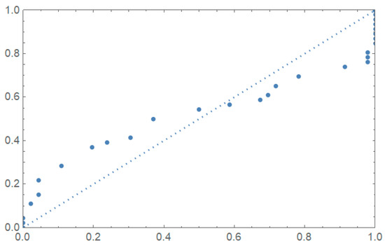
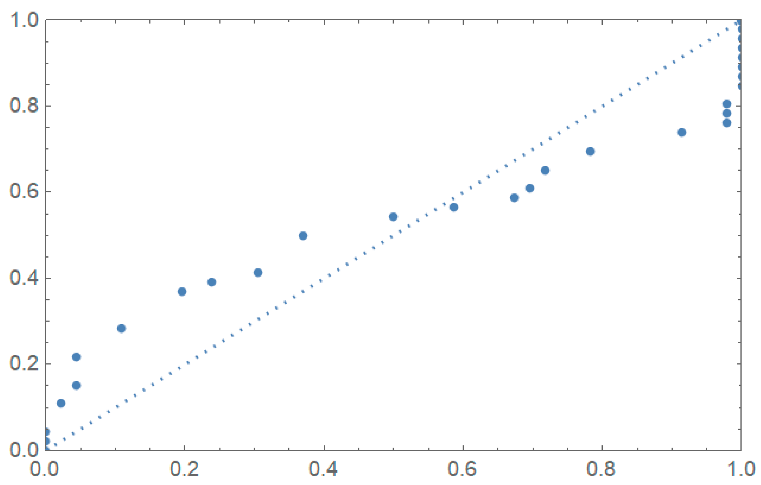
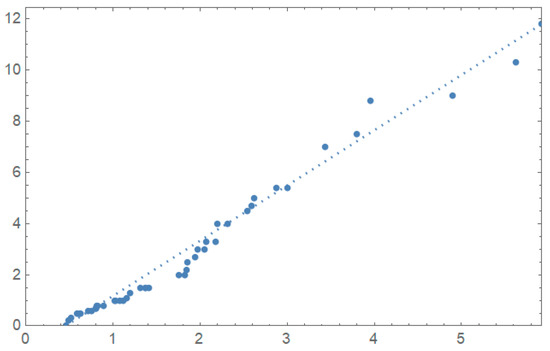
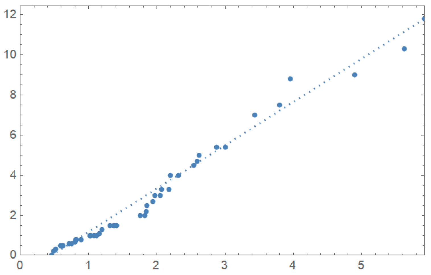
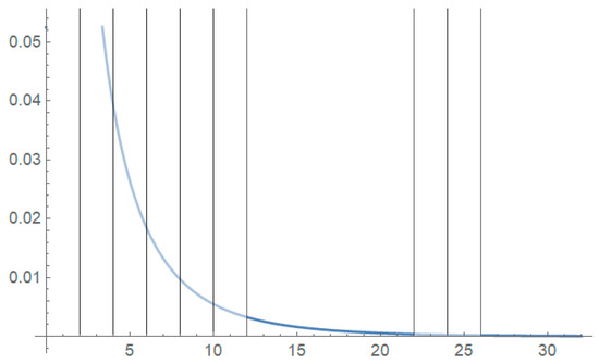
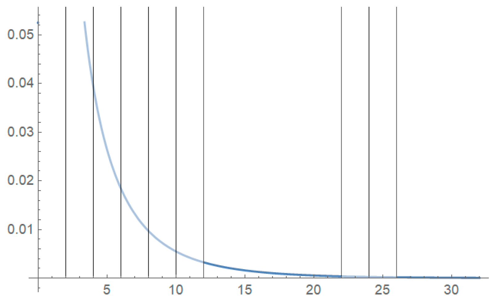
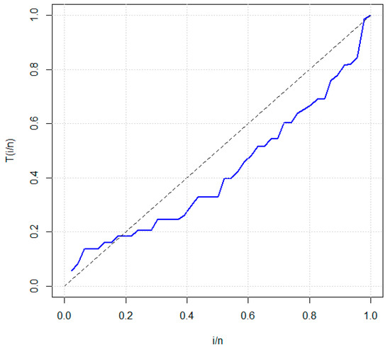
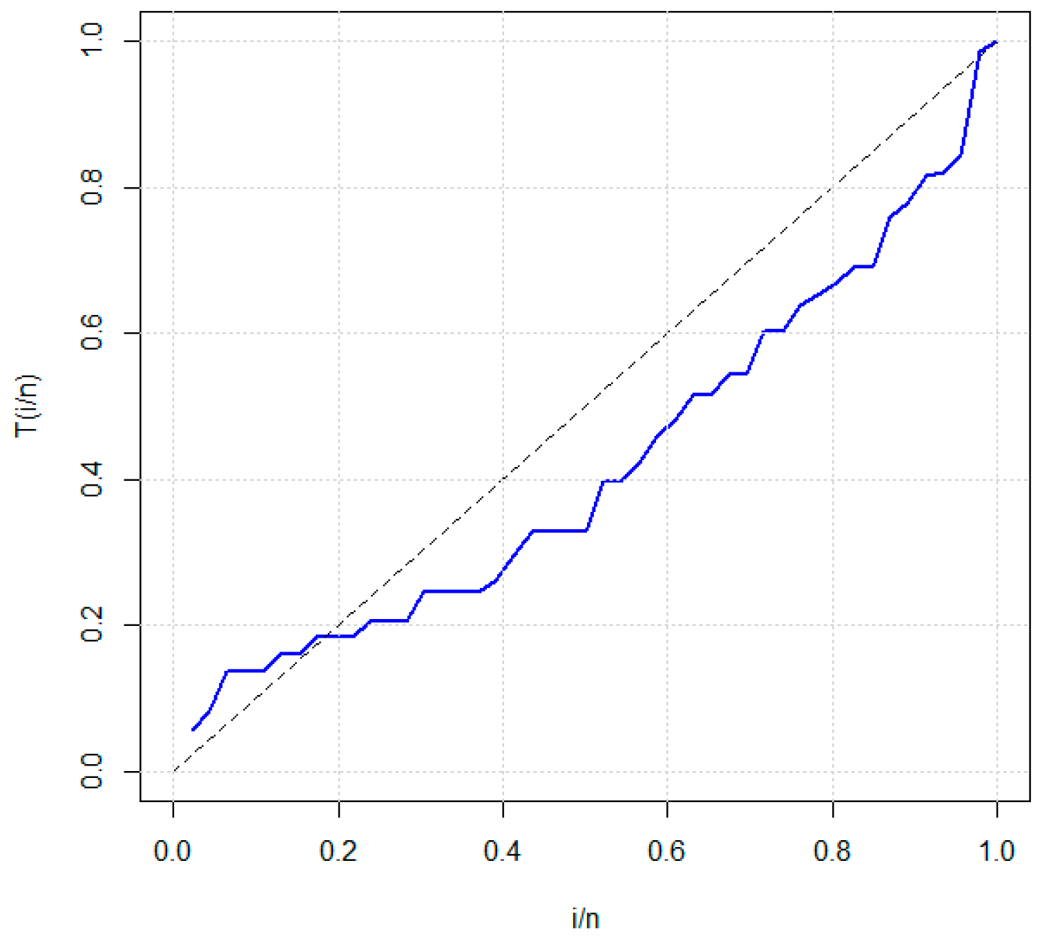
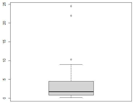
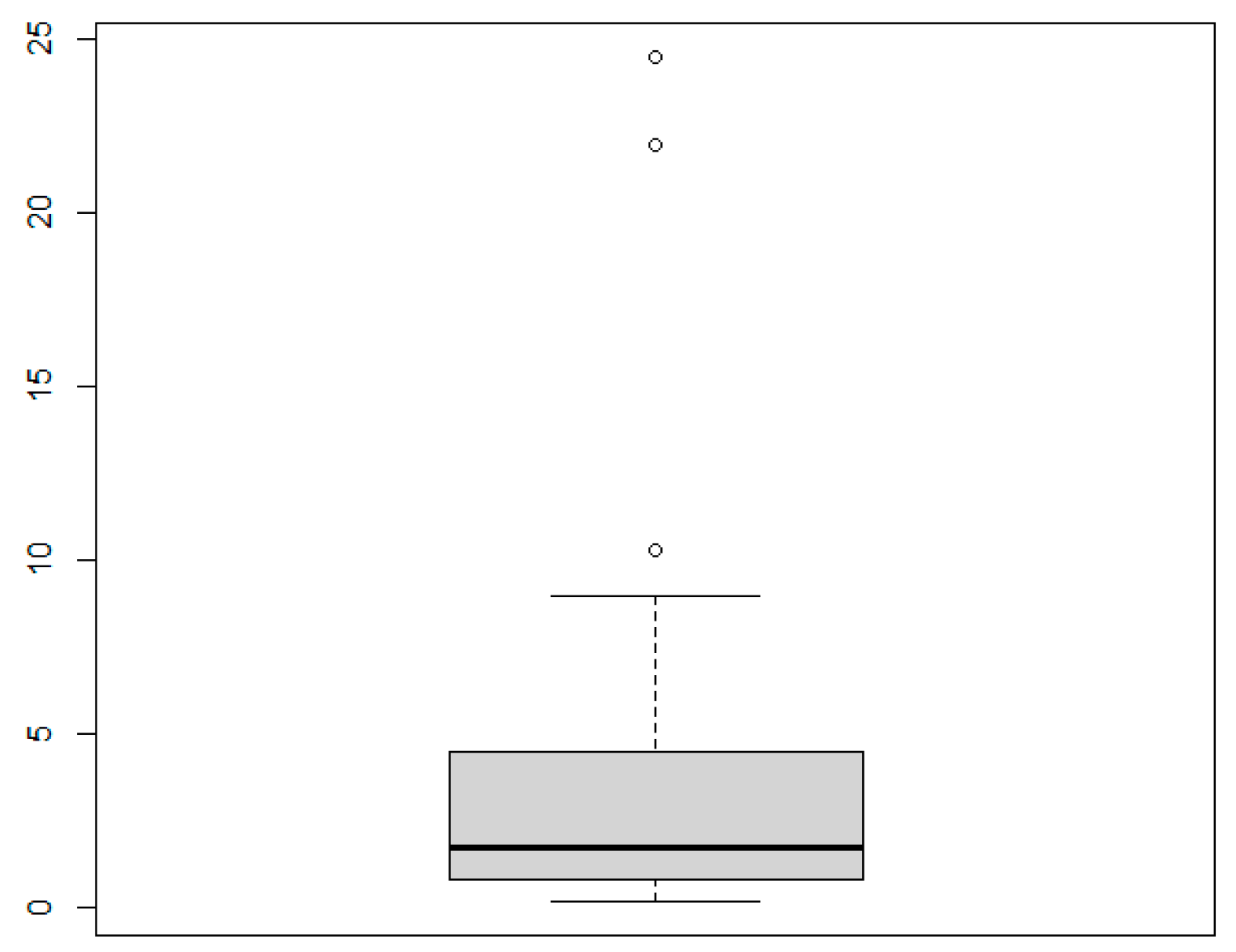
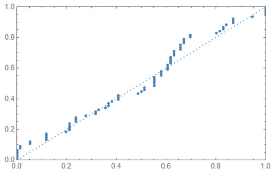
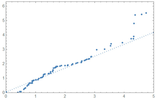
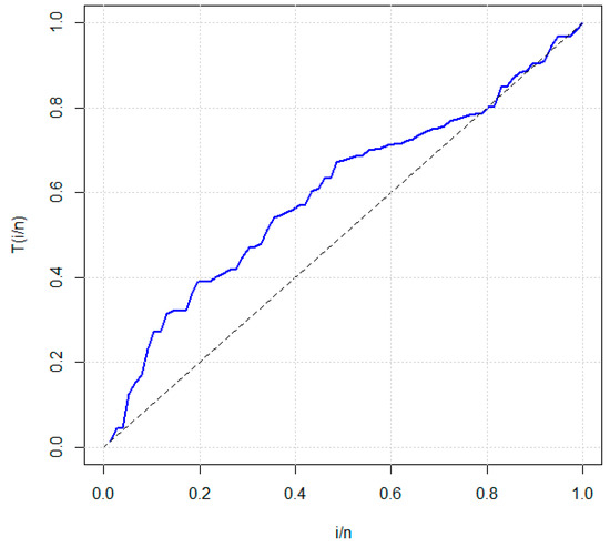
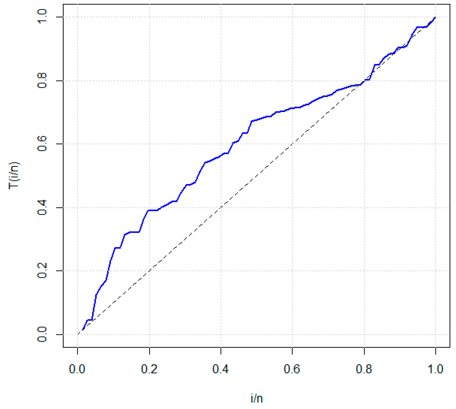
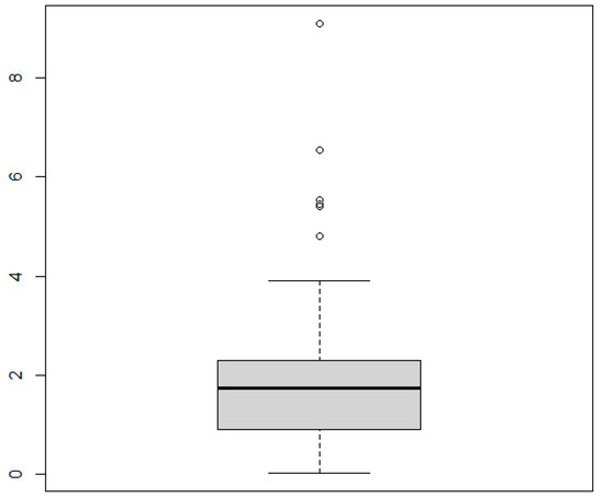
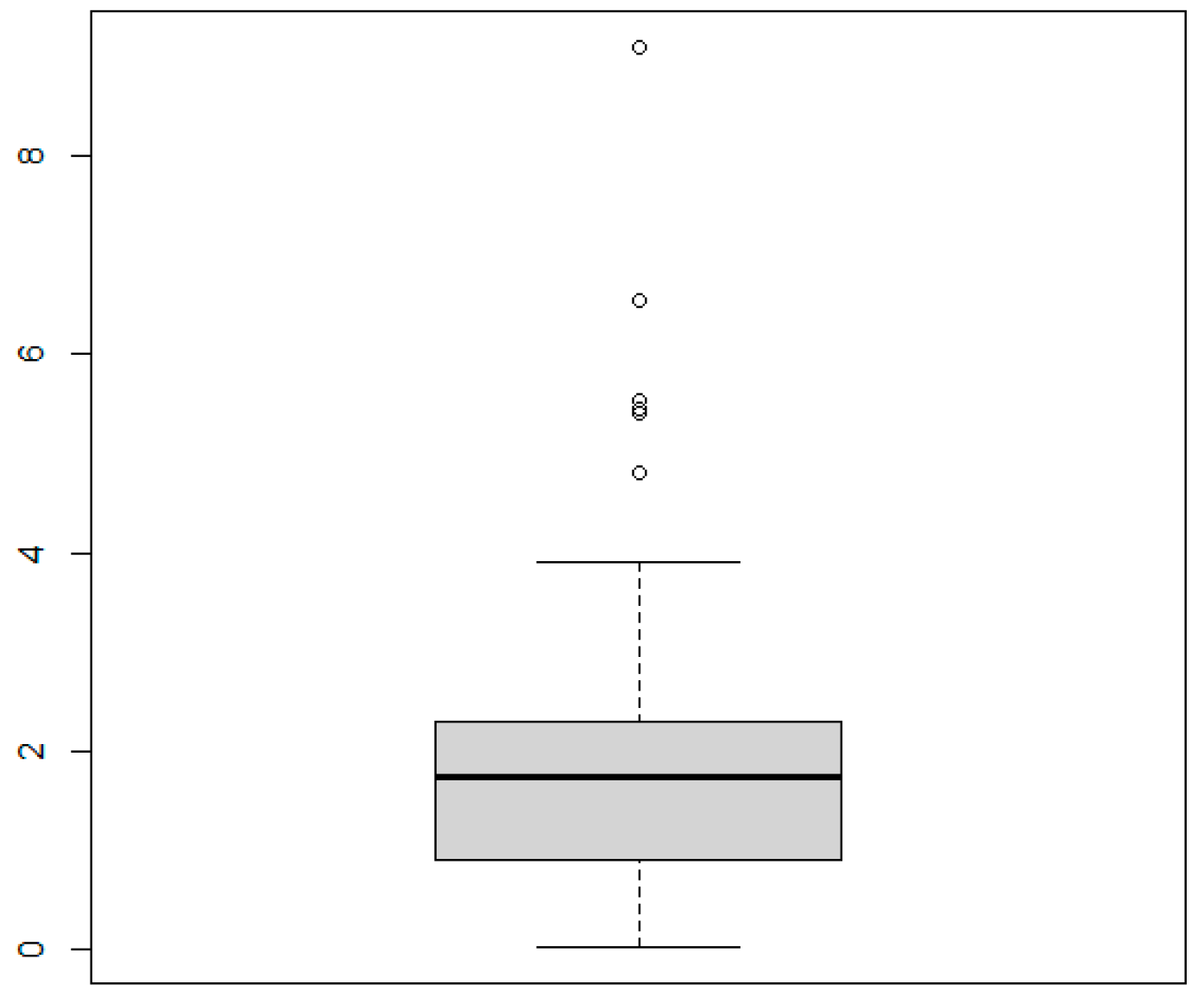
For the first real dataset, Figure 4, Figure 5, Figure 6, Figure 7 and Figure 8 exhibit the P-P plot, Q-Q plot, empirical histogram, empirical scaled TTT-transform plot and boxplot, demonstrating the fit of the MENTL-IW distribution. Figure 9, Figure 10, Figure 11, Figure 12 and Figure 13 provide the corresponding plots for the second dataset.

Figure 4. PP-plot of the MENTL-IW distribution for the first real dataset.

Figure 5. QQ-plot of the MENTL-IW distribution for the first dataset.

Figure 6. Empirical histogram plot for the first dataset.

Figure 7. The empirical scaled TTT-transform plot for the first dataset.

Figure 8. Boxplot for the first dataset.

Figure 9. PP-plot of the MENTL-IW distribution for the second dataset.

Figure 10. QQ-plot of the MENTL-IW distribution for the second dataset.

Figure 11. Empirical histogram plot for distribution for the second dataset.

Figure 12. The empirical scaled TTT-transform plot for the second dataset.

Figure 13. Boxplot for the second dataset.

The datasets were chosen to represent different engineering scenarios and to demonstrate the flexibility and applicability of the proposed distribution in diverse real-world contexts.

Dataset I: The first dataset was taken from [13] This dataset refers to the repair time (hours) of a simple total sample of 46 airborne communications receivers. This dataset was chosen to illustrate the applicability of the proposed distribution in modeling real-world reliability data, specifically in the context of electronic equipment maintenance. The data are

0.2, 0.3, 0.5, 0.5, 0.5, 0.6, 0.6, 0.7, 0.7, 0.7, 0.8, 0.8, 0.8, 1.0, 1.0, 1.0, 1.0, 1.1, 1.3, 1.5, 1.5, 1.5, 1.5, 2.0, 2.0, 2.2, 2.5, 2.7, 3.0, 3.0, 3.3, 3.3, 4.0, 4.0, 4.5, 4.7, 5.0, 5.4, 5.4, 7.0, 7.5, 8.8, 9.0, 10.3, 22.0 and 24.5.

Dataset II: The second dataset represents the life of fatigue fracture of Kevlar 373/epoxy that is subject to constant pressure at the 90% stress level until all had failed, so the data with the exact times of failure were completed. This dataset is taken from [14]. This dataset was selected to demonstrate the model’s flexibility in analyzing data related to material fatigue and lifetime, which are crucial considerations in various engineering applications. The data are as follows:

0.0251, 0.0886, 0.0891, 0.2501, 0.3113, 0.3451, 0.4763, 0.5650, 0.5671, 0.6566, 0.6748, 0.6751, 0.6753, 0.7696, 0.8375, 0.8391, 0.8425, 0.8645, 0.8851, 0.9113, 0.9120, 0.9836, 1.0483, 1.0596, 1.0773, 1.1733, 1.2570, 1.2766, 1.2985, 1.3211, 1.3503, 1.3551, 1.4595, 1.4880, 1.5728, 1.5733, 1.7083, 1.7263, 1.7460, 1.7630, 1.7746, 1.8275, 1.8375, 1.8503, 1.8808, 1.8878, 1.8881, 1.9316, 1.9558, 2.0048, 2.0408, 2.0903, 2.1093, 2.1330, 2.2100, 2.2460, 2.2878, 2.3203, 2.3470, 2.3513, 2.4951, 2.5260, 2.9911, 3.0256, 3.2678, 3.4045, 3.4846, 3.7433, 3.7455, 3.9143, 4.8073, 5.4005, 5.4435, 5.5295, 6.5541 and 9.0960.

The results presented in Table 8 and Table 9 exhibit the superior performance of the MENTL-IW distribution because it consistently exhibits the lowest values for LL, AIC, BIC and CAIC for both real datasets. Furthermore, the MENTL-IW distribution demonstrates the best fit for both datasets, as evidenced by the highest p-values in the goodness-of-fit tests. Furthermore, the results of the comparison between the proposed distribution and each of its components validate superior performance, supporting the theoretical expectations.

Figure 4, Figure 5, Figure 6, Figure 7 and Figure 8 present the empirical scaled TTT-transform, boxplot, histogram, P-P plot and Q-Q plot for the first dataset. The TTT plot indicates an unimodal hazard function. The boxplot and histogram reveal a right-skewed distribution. The P-P and Q-Q plots suggest that the MENTL-IW distribution provides a good fit for the data.

From Figure 4, Figure 5, Figure 6, Figure 7 and Figure 8, one can observe that the MENL-IW distribution fits the first dataset properly. The TTT plot for the first dataset, obtained from [13], exhibits an unimodal shape. This dataset comprises repair times (in hours) for 46 airborne communication receivers. An unimodal TTT plot suggests that the underlying failure rate function may initially increase and subsequently decrease or vice versa. This implies that the repair times may exhibit a pattern where the likelihood of repair initially increases and subsequently decreases, or vice versa.

Figure 9, Figure 10, Figure 11, Figure 12 and Figure 13 display the plot of the empirical scaled TTT-transform of the second dataset, which implies that these data have an increasing hazard function, boxplot and the histogram of the data. One can notice that these data are right-skewed. The P-P plot, Q-Q plot and the fitted MENTL-IW distribution plots indicate that MENTL-IW distribution provides a better fit to these data.

The TTT plot for the second dataset exhibits an increasing hazard rate function, indicating that the likelihood of failure increases over time. This dataset comprises the lifetimes of fatigue fracture of Kevlar 373/epoxy subjected to constant pressure at the 90% stress level until all specimens failed, providing complete failure time data. An increasing hazard rate suggests that the material is more susceptible to failure as time progresses, which is expected behavior under constant stress conditions in fatigue testing.

6. Concluding Remarks

This paper introduces a new family of distributions: the mixture of exponentiated and new Topp–Leone-G family. Some important properties of this family are investigated. As a sub-model, the MENTL-IW distribution is proposed. Statistical properties of the MENTL-IW distribution are derived, including maximum likelihood and Bayesian estimators of the model parameters under both squared error and linear exponential loss functions. Additionally, we estimate the reliability and hazard rate functions. A simulation study evaluates the performance of the ML and Bayesian estimators. The flexibility and applicability of the MENTL-IW distribution are demonstrated through two applications to two real-world engineering datasets. The MENTL-IW distribution consistently exhibits the best fit among the considered models, as shown by the highest p-values in goodness-of-fit tests. Furthermore, comparisons with its essential components validate its superior performance, supporting the theoretical expectation.

7. Suggested Future Work

Future research areas include investigating predictive inference for the proposed MENTL-G family and the MENTL-IW distribution. This contains exploring both non-Bayesian and Bayesian approaches, particularly focusing on one- and two-sample prediction problems. Also, alternative estimation methods beyond maximum likelihood can be explored, such as modified maximum likelihood, E-Bayesian and empirical Bayesian methods, to estimate the model parameters, reliability function and hazard rate function. Moreover, the MENTL-G framework can be extended in several ways: by considering mixtures with more than two components, by substituting different base distributions within the mixture and by exploring the development of new mixture distributions based on this general outline. Furthermore, the robustness of ML and Bayesian estimation procedures can be investigated under various censoring schemes involving Type I, Type II and hybrid censoring. Finally, the application of cluster analysis techniques within the basis of the MENTL-G family and the MENTL-IW distribution presents an exciting path for future research to provide valuable insights into data structures and identify subgroups.

References

- Ahmed, K.E.; Moustafa, H.M.; Abd-Elrahman, A.M. Approximate Bayes estimation for mixture of two Weibull distributions under Type-2 censoring. J. Stat. Comput. Simul. 1997, 58, 269–285. [Google Scholar] [CrossRef] [Scilit]
- AL-Hussaini, E.K.; AL-Dayian, G.R.; Adham, S.A. On finite mixture of two-component Gompertz lifetime model. J. Stat. Comput. Simul. 2000, 67, 20–67. [Google Scholar] [CrossRef] [Scilit]
- Jaheen, Z.F. On record statistics from a mixture of two exponential distributions. J. Stat. Comput. Simul. 2005, 75, 1–11. [Google Scholar] [CrossRef] [Scilit]
- Shawky, A.I.; Bakoban, R.A. On infinite mixture of two component exponentiated gamma distribution. J. Appl. Sci. Res. 2009, 5, 1351–1369. [Google Scholar]
- Dey, S.; Baharith, L.; Alotaibi, R.; Rezk, H.R. The mixture of the Marshall-Olkin extended Weibull distribution under type-II censoring and different loss functions. Math. Probl. Eng. 2021, 2021, 6654101. [Google Scholar]
- Crisci, C.; Perera, G.; Sampognaro, L. Estimating the components of a mixture of extremal distributions under strong dependence. Adv. Pure Math. 2023, 13, 425–441. [Google Scholar] [CrossRef]
- AL-Dayian, G.R.; EL-Helbawy, A.A.; Abd El-Maksoud, F.G. A new mixture of two components of exponentiated family with applications to real life data sets. Comput. J. Math. Stat. Sci. 2024, 3, 258–279. [Google Scholar]
- McLachlan, G.; Peel, D. Finite Mixture Models; John Wiley & Sons, Inc.: Hoboken, NJ, USA, 2000. [Google Scholar]
- Otiniano CE, G.; Gonçalves, C.R.; Dorea, C.C.Y. Mixture of extreme-value distributions: Identifiability and estimation. Commun. Stat. Theory Methods 2017, 46, 6528–6542. [Google Scholar] [CrossRef] [Scilit]
- Gupta, R.C.; Gupta, P.; Gupta, R.D. Modeling failure time data by Lehmann alternatives. Commun. Stat. Theory Methods 1998, 27, 887–904. [Google Scholar] [CrossRef] [Scilit]
- Hassan, A.S.; El-Sherpieny, E.A.; El-Taweel, S.A. New Topp Leone-G family with mathematical properties and applications. J. Phys. Conf. Ser. 2021, 1860, 012011. [Google Scholar] [CrossRef] [Scilit]
- Sultan, K.S.; Ismail, M.A.; Al-Moisheer, A.S. Mixture of two inverse Weibull distributions: Properties and estimation. Comput. Stat. Data Anal. 2007, 51, 5377–5387. [Google Scholar]
- Barahona, J.A.; Gomez, Y.M.; Gomez-Deniz, E.; Venegas, O.; Gomez, H.W. Scale mixture of exponential distribution with an application. Mathematics 2024, 12, 156. [Google Scholar] [CrossRef] [Scilit]
- Gomez, M.Y.; Bolfarine, H.; Gomez, H.W. A New Extension of Exponential Distribution. Rev. Colomb. De Estad. 2014, 37, 25–34. [Google Scholar] [CrossRef] [Scilit]
Disclaimer/Publisher’s Note: The statements, opinions and data contained in all publications are solely those of the individual author(s) and contributor(s) and not of MDPI and/or the editor(s). MDPI and/or the editor(s) disclaim responsibility for any injury to people or property resulting from any ideas, methods, instructions or products referred to in the content. |
© 2025 by the authors. Licensee MDPI, Basel, Switzerland. This article is an open access article distributed under the terms and conditions of the Creative Commons Attribution (CC BY) license (https://creativecommons.org/licenses/by/4.0/).