Abstract
The inverse Gaussian (IG) distribution exhibits asymmetry and right skewness. This distribution presents values uniformly, encompassing wait length, stochastic processes, and rates of accident occurrences. The delta-inverse Gaussian (delta-IG) distribution is suitable for modeling traffic accident data as a mortality count, especially in cases when accidents may not occur. The confidence interval (CI) for the variance and standard deviation of the delta-IG distribution for the accident count is crucial for evaluating risk, allocating resources, and formulating enhancement protocols for transportation safety. We aim to construct confidence intervals for variance and standard deviation in the delta-IG population using several approaches: Adjusted GCI (AGCI), Parametric Bootstrap Percentile CI (PBPCI), fiducial CI (FCI), and Bayesian credible interval (BCI). The AGCI, PBPCI, and FCI will be utilized with estimation methods for proportions which are VST, Wilson’s score, and Hannig approaches. Monte Carlo simulations were evaluated, and the suggested confidence interval approach was employed for the average width (AW) and coverage probability (CP). The findings demonstrated that the AGCI based on the VST method employed successful approaches, as seen in their CP and AW. We employed these approaches to produce CIs for the variance and S.D. of the mortality count in Bangkok.
1. Introduction
Parameter estimation is a fundamental component of statistical inference, widely utilized in theoretical and practical statistics. Population parameters may be expressed as individual values or ranges depending on the purpose of the analytical study. A point estimate derives a singular value for an unknown parameter based on sampled data. Conversely, interval estimation is utilized to establish a range of plausible values for the parameter. Interval estimation entails determining the upper and lower limits that define this range, sometimes using confidence measures. Unlike point estimation, interval estimation requires a comprehensive grasp of the probability distribution and statistical characteristics of the unknown parameter, offering a significant advantage in inferential depth. This study uses interval estimation to compute the confidence interval (CI).
In several fields, including economics, meteorology, biology, and medicine, data characterized by non-negativity and a significant number of zeros are commonly seen. These sorts of data frequently exhibit asymmetry with right-skewed distributions and heteroscedasticity, characterized by a significant presence of both zero and positive values. In traffic accident statistics, counts may be zero if no accident occurs, or they may reflect the number of accidents recorded.
Researchers have investigated several distributions to formulate CIs and address the distinct characteristics of zero-inflated data. Zhou and Tu [1] examined CIs for the means ratio in delta-lognormal populations utilizing maximum likelihood bootstrap methods. Zhang et al. [2] advanced this investigation by computing SCIs for the means ratio of two independent delta-lognormal distributions, employing fiducial and MOVER approaches. Subsequent studies have proposed several approaches for confidence intervals regarding various characteristics of the delta-lognormal distribution.
Nonetheless, Chhikara and Folks [3] have shown that the inverse Gaussian (IG) distribution offers certain advantages over more complex distributions, such as the lognormal distribution. This distribution is very adaptable and computationally more straightforward. Chatzidiamantis et al. [4] have shown its effectiveness in modeling wind speed data and the benefits of parameter estimation. Bardsley [5] compared the IG distribution to the three-parameter Weibull distribution, illustrating its reduced complication.
The zero-inflated inverse Gaussian distribution, sometimes referred to as the delta-inverse Gaussian (delta-IG) distribution, has been employed in several contexts, such as calculating insurance replacement costs, regional precipitation volumes, COVID-19 mortality rates, and daily traffic accident occurrences. Jana and Gautam [6] have focused on CIs for a single mean, mean differences, and mean ratios within the zero-inflated inverse Gaussian framework. Khumpasee, Niwitpong, and Niwitpong [7] investigated the estimation of CI for the coefficient of variation (CV) for delta-IG distributions. Nevertheless, further studies are required to investigate the computation of CIs for variance and standard deviation in this distribution. The coefficient of variation is utilized mostly for comparing the variability between two distinct datasets. The standard deviation and variance of datasets are frequently employed to assess the dispersion of values within a single dataset.
Variance quantifies dispersion by indicating the extent to which data values deviate from the mean. The calculation involves squaring the deviations from the mean, summing these squared deviations, and dividing them by the sample size of the dataset. Variance is essential for assessing diversity across populations. Standard deviation (S.D.) is a fundamental statistical metric that indicates the degree to which data values diverge from the mean. Standard deviation is equal to the square root of the variance. It quantifies the variability within a dataset, where smaller values signify data points around the mean and higher values indicate more dispersion. Prior research has investigated CIs for variance and S.D. across various distributions. Chiou [8] elucidates the formulation of CIs for variance in normal distributions with chi-squared methodologies. Wu [9] examines the construction of CIs for the variance of exponential distributions utilizing the chi-squared method. Paksaranuwat and Niwitpong [10] establish CIs for the variance and variance ratios across multiple distributions in the presence of missing data. Bonett [11] discusses an improved method for calculating confidence intervals for the standard deviation when data do not follow a normal distribution. The paper provides simulation results comparing the proposed method to traditional confidence intervals, demonstrating its superior performance across various nonnormal distributions.
This study intends to calculate and compare CIs for the variance and S.D. of the delta-IG distribution using four approaches. These approaches are evaluated: Adjusted Generalized Confidence Interval (AGCI), Parametric Bootstrap Percentile Confidence Interval (PBPCI), fiducial confidence interval (FCI), and Bayesian credible interval (BCI). Especially, AGCI, PBPCI, and FCI are utilized with estimation methods for the parameter , which are the VST, Wilson’s score, and Hannig techniques. The resultant CIs are assessed across many situations to ascertain their relative effectiveness. The suggested CI approach was assessed for two criteria: average width (AW) and coverage probability (CP) via Monte Carlo simulations. We employed these approaches to produce CIs for the variance of the mortality count in Bangkok for real-life applications.
2. The Confidence Interval for the Variance and Standard Deviation of a Delta-IG Distribution
Let be a random sample from the delta-IG distribution expressed as - where represents the mean, denotes the shape parameter (), and signifies the probability of observing zero value. The probability density function of delta-IG is expressed as
where and . The sample contains observations, separated into zero () and nonzero observations (), such that and follow a binomial distribution denoted as .
The MLEs of and of the distribution are as follows: , , and , respectively. The expected value was , and the variance was . The standard deviation of the distributions is . The variance and S.D. are parameters that we want to estimate for its confidence interval, and we will denote them as
and
respectively.
2.1. AGCI
Weerahandi [12] established the GCI approach based on the Generalized Pivotal Quantity (GPQ) method. The GPQ technique, which is an extension of the Pivotal Quantity (PQ), is dependent on nuisance parameters, whereas the previous may be seen from the perspective of the sample group and the parameters of interest. The nuisance parameter does not influence the observed value of the GPQ method, and the method’s parameters possess unknown values that are independent of any distribution.
Ye, Ma, and Wang [13] introduced a method for constructing CIs for the mean of the IG distribution over many populations via the GPQ method.
The GPQs for and , as introduced by Ye, Ma, and Wang, are given by
where was a chi-square distribution with degrees of freedom and
where is approximately distributed as a standard normal distribution, denoted as .
Following the application of the GCI approach to construct the CIs of the CV for the IG distribution, an additional GPQ for the parameter was identified, as suggested by Krishnamoorthy and Tian [14]. This AGCI approach utilizes another GPQ of the parameter in place of the GPQ for the parameter as presented in (5) of the GCI method. The GPQ for the parameter proposed by Krishnamoorthy and Tian is expressed as
where is Student’s t distribution with degrees of freedom. The algorithm of the AGCI method is defined in Algorithm 1.
| Algorithm 1: AGCI | |
| 1. | . |
| 2. | from chi-square and Student’s t distributions, respectively. |
| 3. | using (4) and (6), respectively. |
| 4. | = 1, 2, …, 5000 times. |
2.1.1. AGCI Based on the VST Method
The VST approach was first presented by Dasgupta [15], using the normal approximation. Wu and Hsieh [16] devised the variance-stabilizing transformation (VST) for a binomial distribution, approximating it using the arcsine square-root transformation. Thus, the GPQ for , as articulated by Wu and Hsieh, is delineated as
where , .
Hence, the GPQs of the parameters were , , and , expressed as (4), (6), and (7), respectively. The GPQ for is given by
The 100(1 − )% two-sided CI for using the AGCI based on the VST method is
where and are the -th and -th percentiles of the distribution of , respectively.
And the GPQ for is given by
The 100(1 − )% two-sided CI for using the AGCI based on the VST method is
where and are the -th and -th percentiles of the distribution of , respectively.
2.1.2. AGCI Based on Wilson’s Score Method
Wilson [17] introduced Wilson’s score CI for estimating the CI of proportions. Then, Li, Zhou, and Tian [18] achieved the GPQ for as
where was the standard normal distribution.
Hence, the GPQs of the parameters were , , and , expressed as (4), (6), and (12), respectively. The GPQ for is given by
The 100(1 − )% two-sided CI for using the AGCI based on Wilson’s score method is
where and are the -th and -th percentiles of the distribution of , respectively.
And the GPQ for is given by
The 100(1 − )% two-sided CI for using the AGCI based on Wilson’s score method is
where and are the -th and -th percentiles of the distribution of , respectively.
2.1.3. AGCI Based on the Hannig Method
Hannig [19] presented the GFQ of . A prior study indicates that the optimal GFQ for is the product of two beta distributions, each assigned a weight of 0.5. Following this, the study conducted by Li, Zhou, and Tian [20] employed the earlier documented GFQ. Additionally, it is consistent with the GPQ idea. The GPQ for from Hannig is
Hence, the GPQs of the parameters were , , and , expressed as (4), (6), and (17), respectively. The GPQ for is given by
The 100(1 − )% two-sided CI for using the AGCI based on the Hannig method is
where and are the -th and -th percentiles of the distribution of , respectively.
And the GPQ for is given by
The 100(1 − )% two-sided CI for using the AGCI based on the Hannig method is
where and are the -th and -th percentiles of the distribution of , respectively.
2.2. PBPCI
The PBPCI method was established in the study of Efron and Tibshirani [20] by applying resampling techniques called bootstrap techniques, which derive resampled data from the original dataset. Each distribution is assessed to investigate the characteristics that define the predicted statistics. This study employed the PBPCI method to compute confidence intervals, utilizing 1000 resamples. This PBPCI method will utilize the methods of estimation for the parameter with three methods (VST, Wilson’s score, and Hannig), the same as in the previous approach, to establish the CIs for for the delta-IG distribution. The algorithm of this approach is defined in Algorithm 2.
The 100(1 − )% two-sided CI of for the delta-IG distribution based on the PBPCI method is given by
where and are the -th and -th percentiles of the distribution of .
The 100(1 − )% two-sided CI of for the delta-IG distribution based on the PBPCI method is given by
where and are the -th and -th percentiles of the distribution of .
| Algorithm 2: PBPCI | |
| 1. | . |
| 2. | achieved in step 1. |
| 3. | and from the bootstrap sample. |
| 4. | Repeat steps 2–3 a total of 1000 times. |
| 5. | using (22) and (23). |
2.3. FCI
Fiducial confidence intervals in estimation involve generating a probability distribution for an unknown variable based directly on observable data. This approach is applied without utilizing prior distributions in repeated sampling. This method was introduced in the research conducted by Fisher [21]. The resulting fiducial confidence intervals provide an estimation of the parameter’s intention. This interval is similar to a Bayesian credible interval but does not require objective or subjective priors. While providing a novel perspective on interval estimates, the fiducial method is frequently scrutinized for its unconventional treatment of parameter uncertainty.
The Gibbs sampling technique, as established in Geman and Geman [22], is relevant for fiducial inference. The sample distributions of the maximum likelihood estimates for the parameters and are employed in the delta-IG distribution. The fiducial distribution for the parameters and can be derived by substituting their maximum likelihood estimates (MLEs). When the sample distribution contains both parameters, they are distributed as and , where are the MLEs of and , respectively. This FCI method will utilize the methods of estimation for the parameter with three methods (VST, Wilson’s score, and Hannig), the same as in the previous approaches, to estimate the CIs for for the delta-IG distribution.
The 100(1 − )% two-sided CI of and for the delta-IG distribution based on the FCI method is given by Algorithm 3 with
and
respectively.
| Algorithm 3: FCI | |
| 1. | Set the initial values (MLEs) of parameters |
| 2. | Produce and . |
| 3. | Repeat step 2 a total of = 1, 2, …, 20,000 times, in which is the number of replications of MCMC. |
| 4. | Burn in 1000 samples and compute for the parameter of interest. |
| 5. | Earn and using (24) and (25). |
2.4. BCI
Bayesian credible interval was established based on the Bayesian method. It is a systematic technique used for estimating parameters. The estimator is formulated by integrating a prior distribution with a likelihood function derived from random sample data. The delta-IG distribution function must be integrated with the prior density function to ascertain the posterior density function for the variance and S.D. of the delta-IG population. The likelihood function for the delta-IG distribution is expressed as follows.
where , and .
The posterior density of is given by
Nonetheless, the posterior distributions acquired from the delta-IG distribution are challenging to solve. Thus, we employed the Markov Chain Monte Carlo simulation (MCMC) utilizing Gibbs sampling to furnish them with the parameter. We utilized the Markov Chain Monte Carlo simulation to calculate the single variance, assuming a uniform prior distribution for the parameter , a gamma distribution for the parameter , and a beta distribution for the parameter . Since this method has a prior distribution for estimating the parameter , then the three methods of estimation for the parameter (VST, Wilson’s score, and Hannig) will not be used. This method was computed via the R2OpenBUGS package within the R programming language.
The 100(1 − )% two-sided CI of and for the delta-IG distribution based on the BCI method is given by Algorithm 4 with
and
respectively.
| Algorithm 4: BCI | |
| 1. | . |
| 2. | Assume the prior distribution of each parameter as , , and by trial hyperparameters. |
| 3. | Utilize Gibbs sampling via R programming to produce posterior distribution for three parameters . |
| 4. | . |
| 5. | = 20,000 times. |
| 6. | Burn in 5000 samples. |
| 7. | using (28) and (29). |
3. Simulation Studies
The study considered these approaches for establishing confidence intervals for the variance and S.D. in the delta-IG distribution. The study utilized a Monte Carlo simulation conducted in the R programming language. The approaches were assessed by analyzing their coverage probabilities (CPs) and average widths (AWs). Selecting an optimal strategy depends on two critical criteria: the CPs of the method must be close to or exceed the nominal confidence level of 0.95, and the AWs of each approach should be evaluated to determine the narrowest width. The simulation was run using a total of 5000 iterations. Sample data for the variance and standard deviation of the delta-IG distribution were produced for by the - distribution. The sample sizes () were 30, 50, 100, and 200. The mean () was determined to be either 0.5 or 1.0. The shape parameter () was set at 1, 2, 5, and 10. The probability () was set at 0.3 and 0.5.
4. Results
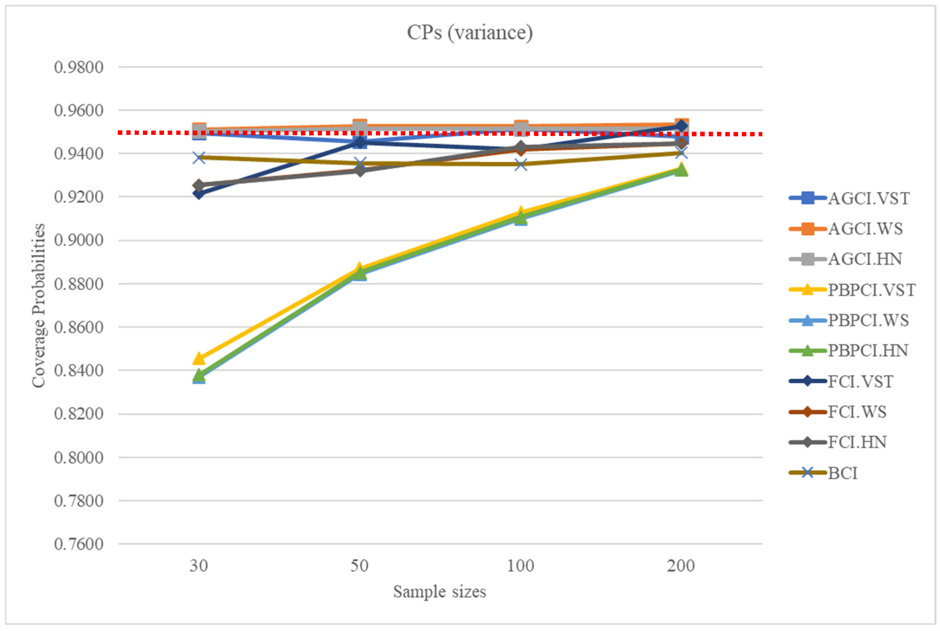
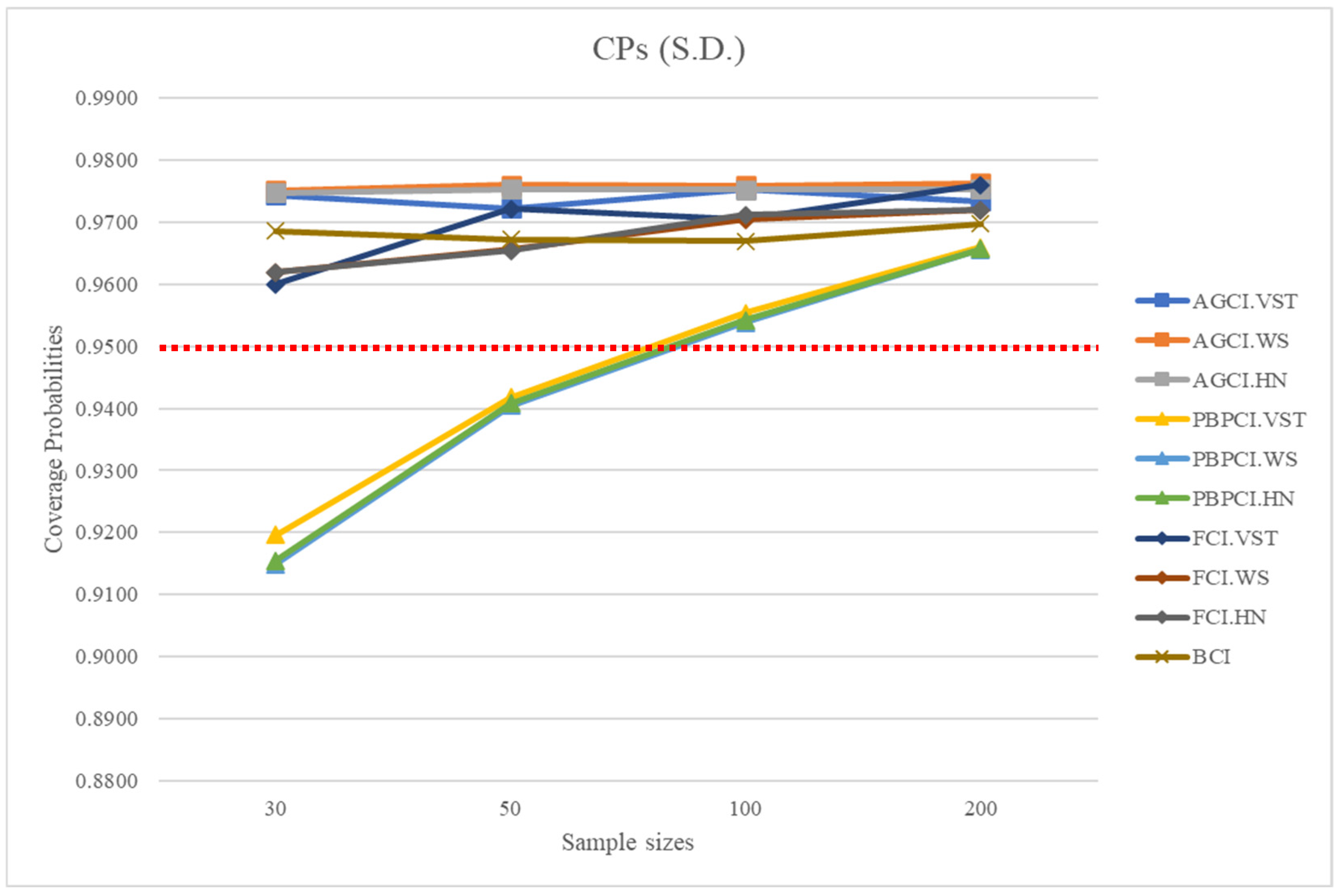
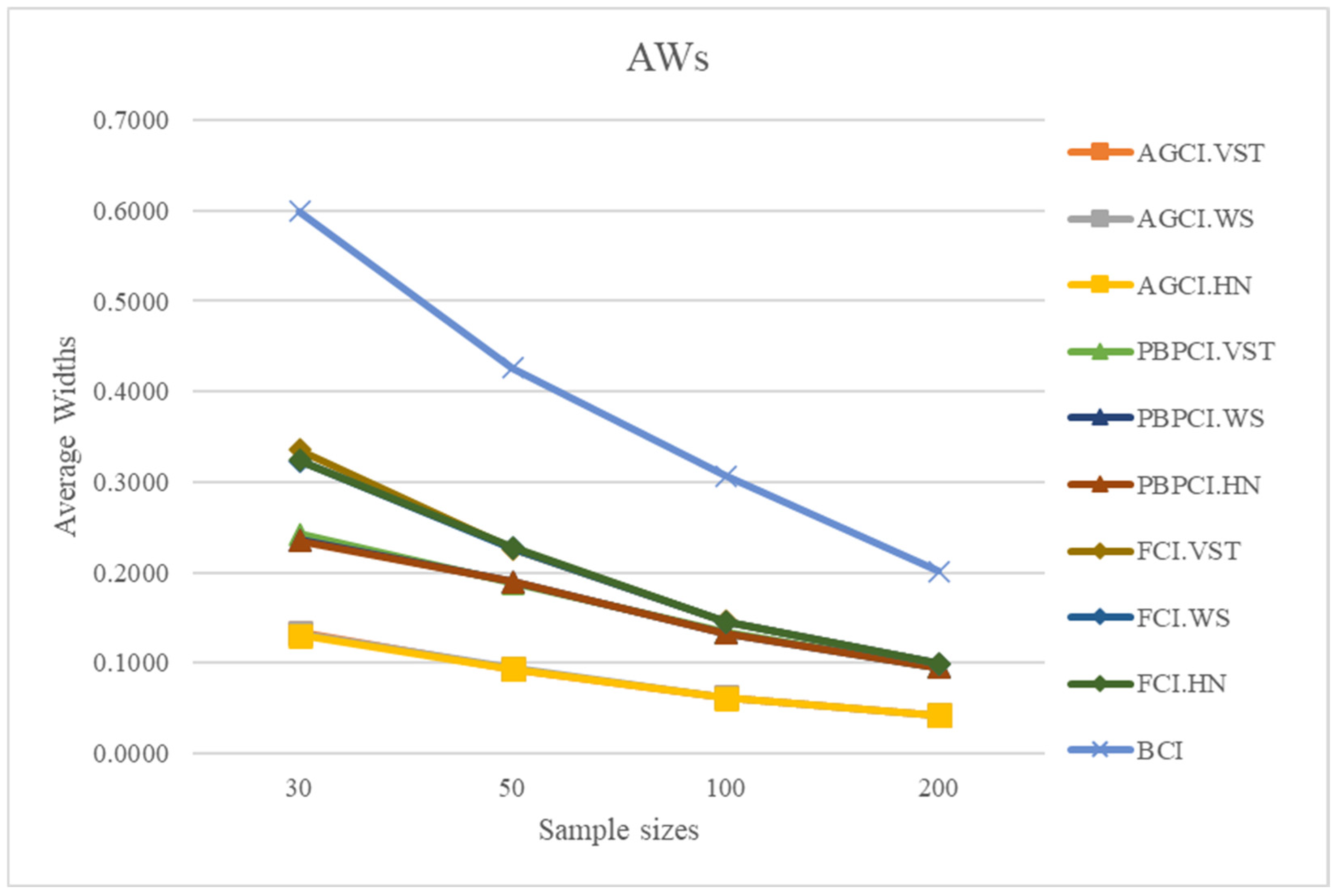
The findings from Table 1, Table 2 and Table 3 regarding CPs and AWs are visually represented as Figure 1 for the CPs of CIs for variance, Figure 2 for the CPs of CIs for S.D., and Figure 3 for AWs. The red dotted line in Figure 1 and Figure 2 represents the line of nominal coverage level of 0.95. However, the table of AWs from the confidence intervals of standard deviation were omitted as the findings closely resemble the AWs from the confidence intervals of variance. These representations demonstrate that the CPs from the CI for variance obtained by the AGCI approaches were greater than or close to the nominal confidence level of 0.95 in nearly all cases. But when the sample sizes were large, the CPs of the FCI based on the Wilson’s score method were also greater than or close to the nominal confidence level. When comparing the three methods of estimation for the parameter coordinate with the AGCI approach, the CPs of the AGCI based on the VST and Wilson’s score methods were greater than or close to the nominal confidence level of 0.95 than the AGCI based on the Hannig method. For the CPs from the CI for S.D., the CPs obtained by the AGCI, FCI, and BCI approaches were greater than or close to the nominal confidence level of 0.95 for nearly all cases. And when the sample sizes were larger ( = 100 and 200), the PBPCI method also performed better. However, the increasing CP in the PBPCI method with larger sample sizes (Figure 1 and Figure 2) is due to several statistical factors. According to the Law of Large Numbers (LLN), larger samples yield more accurate parameter estimates, reducing variance and improving confidence intervals. PBPCI benefits from probability-based estimation, where larger datasets provide more stable distributions, minimizing randomness and bias. Other methods may not show a clear trend due to their differences in numeric value. When assessing the average widths, the AGCI based on the VST method had the smallest width among the others, followed by AGCI based on the Hannig method, AGCI based on the Wilson’s score method, and PBPCI, FCI, and BCI approaches. While assessing two criteria simultaneously, the method that showed an outstanding performance was the AGCI based on the VST method.

Table 1.
The coverage probabilities of the 95% confidence intervals for the variance of delta-IG distributions.
Table 2.
The coverage probabilities of the 95% confidence intervals for the standard deviation of delta-IG distributions.
Table 3.
The average widths of the 95% confidence intervals for the variance of delta-IG distributions.
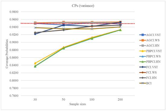
Figure 1.
Comparison of coverage probabilities of proposed CIs for variance with various sample sizes: .
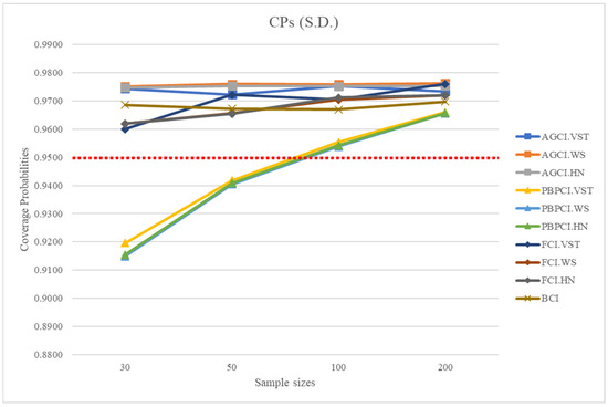
Figure 2.
Comparison of coverage probabilities of proposed CIs for standard deviation (S.D.) with various sample sizes: .

Figure 3.
Comparison of average widths of proposed CIs with various sample sizes: .
5. An Empirical Application
Security planning in transportation and the assessment of transportation infrastructure rely on the statistical study of accident incidence rates. The accuracy of previous models necessitates improvement to tackle several issues associated with collision counts, particularly the widespread occurrence of inflated zero accident figures.
The objective of establishing the confidence interval for the variance and standard deviation of a delta-IG population regarding traffic accident incidence counts is to ascertain the relative dispersion of events. These statistics denote quantitative metrics employed to assess the variability within a dataset or numerous datasets. This study offers significant new insights into the forecasting and sustainability of accident incidence frequency. The aim of the study on calculating the CI of variance and standard deviation is to evaluate risk, allocate resources, and establish enhancement protocols for transportation security.
This study examines data from a statistical report on casualties resulting from traffic accidents, produced by the Road Accident Victims Protection Company Limited, accessible on the Thai RSC website at https://www.thairsc.com/bangkok-in-depth-statistics (accessed on 10 November 2024). The fatality tally from vehicular incidents in December 2023 throughout 50 districts of Bangkok, Thailand, is as follows: 9, 5, 3, 2, 1, 1, 0, 9, 4, 2, 2, 2, 1, 0, 5, 5, 3, 2, 1, 1, 1, 0, 0, 3, 2, 2, 1, 1, 1, 1, 0, 4, 2, 2, 1, 1, 0, 0, 0, 0, 4, 3, 1, 1, 0, 0, 0, 0, 0. The aim is to illustrate the efficacy of the CIs for the variance and standard deviation of delta-IG distributions derived from these techniques.
The positive values of the data can be represented using asymmetric distributions. We analyzed the distributions of datasets with positive mortality counts utilizing the Akaike Information Criterion (AIC) and the Bayesian Information Criterion (BIC), defined as
and
respectively, where the likelihood function is denoted as , represents the number of parameters, and indicates the number of observations.
Table 4 facilitates the identification of the most suitable distribution for the dataset by presenting the AIC and BIC values for asymmetric distributions. The mortality dataset in Bangkok seems to adhere to an inverse Gaussian distribution, and when including zero values, it aligns with a delta-inverse Gaussian distribution, as indicated by the lowest AIC and BIC values for the inverse Gaussian distribution.
Table 4.
AIC and BIC values for the fitting of nine asymmetric distributions.
Table 5 presents the computed descriptive statistics for the mortality data in Bangkok. The variance was 3.7619 and the standard deviation was 1.9396. Table 6 displays the 95% CIs for variance and the 95% CIs for S.D. obtained from the proposed methods. The findings indicated that the AW of BCI was the shortest. However, Bayesian intervals, which may be tailored based on prior information, may yield narrower intervals than alternative approaches since selecting prior distributions from the dataset might result in shorter credible intervals. After that, the AGCI approaches yield a shorter average width than other techniques. Following the evaluation of the CPs and AWs criteria through simulation studies and an empirical application, the AGCI utilizing the VST technique was deemed appropriate for establishing the CI of variance and S.D. for the delta-IG distribution.
Table 5.
Fundamental statistics for the death count data in Bangkok.
Table 6.
The 95% confidence intervals for variance and S.D. from death count in the Bangkok dataset.
6. Conclusions
This study analyzed four approaches to determine an exceptional way to construct CIs for the variance and S.D. of delta-IG distributions. The results of the simulation analysis demonstrate that the CPs from the CI for variance obtained by the AGCI approaches were generally greater than or close to the nominal confidence level of 0.95. For large sample sizes, the FCI based on the Wilson’s score method also performed similarly. Comparing the three estimation methods for the parameter , the AGCI based on the VST and Wilson’s score methods outperformed the AGCI based on Hannig’s method. For the CI of S.D., the AGCI, FCI, and BCI approaches consistently achieved CPs near or above 0.95, with the PBPCI method showing an improved performance for larger sample sizes ( = 100 and 200). The assessment of the AWs indicated that the AGCI utilizing the VST method exhibited the narrowest width compared to the others. However, while evaluating both criteria of CPs and AWs, the AGCI utilizing the VST approach demonstrated outstanding results.
There is an impact of various parameter settings: Large sample sizes ( = 100, 200) enhance accuracy and precision by decreasing variability confidence interval estimations and stabilizing parameter estimation. And small sample sizes ( = 30, 50) typically yield wider confidence intervals with more variability, particularly for method depending on resampling technique such as PBPCI method. For the shape parameter (), when increasing the values of , the skewness reduces and enhances the accuracy of confidence interval estimates, whereas decreased values of lead to more skewed distributions, hence impacting precision. When = 0.3, the number of zero observations in the sample was small, resulting in more consistent estimates of variance and standard deviation. When = 0.5, an increase in the proportion of zero values amplifies variability, complicating the calculation of variance and standard deviation. Techniques such as AGCI and FCI often exhibit superior performance in these instances, but bootstrap-based approaches like PBPCI demonstrate more sensitivity to the variation in .
In an empirical analysis of mortality data in Bangkok, the BCI had the narrowest average width, hence demonstrating the efficacy of these methods. Bayesian intervals, which are informed by prior information, may provide shorter intervals than alternative approaches, since the selection of prior distributions from the dataset might result in narrower credible intervals. After that, the AGCI methods produce a narrower average width compared to alternative procedures. The simulated study and an empirical application indicated that the AGCI utilizing the VST method was the most appropriate method.
To enhance the use of delta-IG in meteorology, health, biology, and economics, it is essential to determine a suitable approach for precisely measuring confidence intervals for variance. This work extended the computation of CIs for the variance and S.D. of the IG distribution to the delta-IG distribution, which is more relevant to practical applications. Consequently, the AGCI based on the VST technique is appropriate for determining the CIs for the variance and S.D. of delta-IG, as demonstrated by a simulation study and empirical application.
7. Discussion
Comprehending mortality statistics is essential for assessing risk, optimizing resource distribution, and formulating effective measures to improve transportation security and sustainability. Research conducted by Seresirikachorn et al. [23] underscores the essential importance of the fair distribution of healthcare resources in mitigating and decreasing road traffic fatalities. By tackling inequities and concentrating on resource distribution, policymakers may formulate more effective plans to improve road safety and decrease deaths throughout Thailand. Consequently, precise measurement of death figures is essential for efficient risk evaluation and the improvement of transportation security management. This work seeks to quantify the confidence intervals for the variation in traffic mortality counts to mitigate these concerns.
This research aimed to estimate the confidence interval for the variance and S.D. of the delta-IG distribution using the described approaches. The simulation results demonstrate that the confidence probabilities of AGCI were continuously more than or about equal to the nominal confidence level of 0.95. This aligns with prior studies conducted by Chankham, Niwitpong, and Niwitpong [24] and Khumpasee, Niwitpong, and Niwitpong [7].
This research calculates the confidence interval for the variance and S.D. of the delta-IG distribution. Future studies may extend these methods to include simultaneous confidence intervals for any pairwise differences or ratios among the variances or standard deviation of multiple delta-IG distributions.
Author Contributions
Conceptualization, W.K., S.-a.N. and S.N.; methodology, W.K. and S.-a.N.; software, W.K.; validation, S.-a.N. and S.N.; formal analysis, S.N.; investigation, S.-a.N. and S.N.; resources, W.K.; data curation, W.K.; writing—original draft, W.K.; preparation, W.K.; writing—review and editing, S.-a.N. and S.N.; visualization, W.K.; supervision, S.-a.N. and S.N.; project administration, S.-a.N.; funding acquisition, S.-a.N. All authors have read and agreed to the published version of the manuscript.
Funding
This research was funded by the National Science, Research and Innovation Fund (NSRF) and King Mongkut’s University of Technology North Bangkok: KMUTNB-FF-68-B-43.
Data Availability Statement
Data are contained within the article.
Acknowledgments
The authors express gratitude to King Mongkut’s University of Technology North Bangkok for providing the opportunity and resources for research. The authors express our sincere gratitude to the editor and the reviewers for thoroughly reviewing our manuscript and recommending essential information to enhance the completeness of our work.
Conflicts of Interest
The authors declare no conflicts of interest.
References
- Zhou, X.H.; Tu, W. Interval estimation for the ratio in means of log-normally distributed medical costs with zero values. Comput. Stat. Data Anal. 2000, 35, 201–210. [Google Scholar] [CrossRef]
- Zhang, Q.; Xu, J.; Zhao, J.; Liang, H.; Li, X. Simultaneous confidence intervals for ratios of means of zero-inflated log-normal populations. J. Stat. Comput. Simul. 2022, 92, 1113–1132. [Google Scholar] [CrossRef]
- Chhikara, R.S.; Folks, J.L. The inverse Gaussian distribution as a lifetime model. Technometrics 1977, 19, 461–468. [Google Scholar] [CrossRef]
- Chatzidiamantis, N.D.; Sandalidis, H.G.; Karagiannidis, G.K.; Kotsopoulos, S.A. On the inverse Gaussian shadowing. In Proceedings of the 2011 International Conference on Communications and Information Technology (ICCIT), Aqaba, Jordan, 29–31 March 2011; pp. 142–146. [Google Scholar]
- Bardsley, W.E. Note on the use of the inverse Gaussian distribution for wind energy applications. J. Appl. Meteorol. 1980, 19, 1126–1130. [Google Scholar] [CrossRef]
- Jana, N.; Gautam, M. Confidence intervals of difference and ratio of means for zero-adjusted inverse Gaussian distributions. Commun. Stat.—Simul. Comput. 2024, 53, 3302–3326. [Google Scholar] [CrossRef]
- Khumpasee, W.; Niwitpong, S.A.; Niwitpong, S. Confidence Intervals for the Coefficient of Variation in Delta Inverse Gaussian Distributions. Symmetry 2024, 16, 1488. [Google Scholar] [CrossRef]
- Chiou, P. Confidence intervals for the variance and standard deviation in normal distribution. Int. J. Contemp. Math. Sci. 2007, 2, 973–982. [Google Scholar]
- Wu, Z. Confidence intervals of variance components for exponential distribution. Commun.Stat.—Theory Methods 2011, 40, 3536–3545. [Google Scholar]
- Paksaranuwat, P.; Niwitpong, S.A. Confidence intervals for the variance and the ratio of two variances of non-normal distributions with missing data. Thail. Stat. 2011, 8, 81–92. [Google Scholar]
- Bonett, D. Approximate confidence interval for standard deviation of nonnormal distributions. Comput. Stat. Data Anal. 2006, 50, 775–782. [Google Scholar] [CrossRef]
- Weerahandi, S. Generalized confidence intervals. J. Am. Stat. Assoc. 1993, 88, 899–905. [Google Scholar] [CrossRef]
- Ye, R.D.; Ma, T.F.; Wang, S.G. Inferences on the common mean of several inverse Gaussian populations. Comput. Stat. Data Anal. 2010, 54, 906–915. [Google Scholar] [CrossRef]
- Krishnamoorthy, K.; Tian, L. Inferences on the difference and ratio of the means of two inverse Gaussian distributions. J. Stat. Plan. Inference 2008, 138, 2082–2089. [Google Scholar] [CrossRef]
- Dasgupta, A. Asymptotic Theory of Statistics and Probability; Springer: New York, NY, USA, 2008. [Google Scholar]
- Wu, W.H.; Hsieh, H.N. Generalized confidence interval estimation for the mean of delta-lognormal distribution: An application to New Zealand trawl survey data. J. Appl. Stat. 2014, 41, 1471–1485. [Google Scholar] [CrossRef]
- Wilson, E.B. Probable inference the law of succession and statistical inference. J. Am. Stat. Assoc. 1927, 22, 209–212. [Google Scholar] [CrossRef]
- Li, X.; Zhou, X.; Tian, L. Interval estimation for the mean of lognormal data with excess zeros. Stat. Probab. Lett. 2013, 83, 2447–2453. [Google Scholar] [CrossRef]
- Hannig, J. On generalized fiducial inference. Stat. Sin. 2009, 19, 491–544. [Google Scholar]
- Efron, B.; Tibshirani, R. Bootstrap methods for standard errors, confidence intervals, and other measures of statistical accuracy. Stat. Sci. 1986, 1, 54–77. [Google Scholar] [CrossRef]
- Fisher, R.A. Inverse probability. Proc. Camb. Philos. Soc. 1930, 26, 528–535. [Google Scholar] [CrossRef]
- Geman, S.; Geman, D. Stochastic relaxation, Gibbs distributions, and the Bayesian restoration of images. IEEE Trans. Pattern Anal. Mach. Intell. 1984, 6, 721–741. [Google Scholar] [CrossRef]
- Seresirikachorn, K.; Singhanetr, P.; Soonthornworasiri, N.; Amornpetchsathaporn, A.; Theeramunkong, T. Characteristics of road traffic mortality and distribution of healthcare resources in Thailand. Sci. Rep. 2022, 12, 20255. [Google Scholar] [CrossRef] [PubMed]
- Chankham, W.; Niwitpong, S.A.; Niwitpong, S. Confidence intervals for the difference between the coefficients of variation of inverse Gaussian distributions. In Integrated Uncertainty in Knowledge Modelling and Decision Making; Lecture Notes in Computer Science; Springer: Berlin/Heidelberg, Germany, 2020; Volume 12482, pp. 401–413. [Google Scholar] [CrossRef]
Disclaimer/Publisher’s Note: The statements, opinions and data contained in all publications are solely those of the individual author(s) and contributor(s) and not of MDPI and/or the editor(s). MDPI and/or the editor(s) disclaim responsibility for any injury to people or property resulting from any ideas, methods, instructions or products referred to in the content. |
© 2025 by the authors. Licensee MDPI, Basel, Switzerland. This article is an open access article distributed under the terms and conditions of the Creative Commons Attribution (CC BY) license (https://creativecommons.org/licenses/by/4.0/).