Edge-Irregular Reflexive Strength of Non-Planar Graphs

Abstract

Symmetry in non-planar graphs is a fundamental concept that enhances understanding, simplifies analyses, and has practical implications in diverse fields such as science, engineering, and mathematics. A total $\kappa$-labeling for a graph $\check{G_{\nu }}$ is composed of two labeling: one is an edge labeling ${{\rm Y}}_e:E(\check{G_{\nu }})\to \{1,2,3,\dots ,{\kappa }_e\}$ and the other is a vertex labeling ${{\rm Y}}_v:V(\check{G_{\nu }})\to \{0,2,4,\dots ,2{\kappa }_v\}$, where $\kappa =max\{{\kappa }_e,2{\kappa }_v\}$. The weight of an edge under reflexive labeling is defined as $wt(pq)={{\rm Y}}_v(p)+{{\rm Y}}_e(pq)+{{\rm Y}}_v(q)\forall e=pq$. The total $\kappa -labeling$ is said to be an edge-irregular reflexive $\kappa -labeling$, if for every two edges $e_{\delta }$ and $e_j$, the weights are distinct. The lowest value of $\kappa$ for which the graph $\check{G_{\nu }}$ has an irregular reflexive edge $\kappa -labeling$ is called the reflexive edge strength of $\check{G_{\nu }}$, denoted as $res(\check{G_{\nu }})$. $res(\check{G_{\nu }})$ captures irregularity while preserving reflexivity by quantifying edge-weight variability in reflexive graphs. In this article, we are interested in determining the tight lower bound for non-planar prisms, cross prisms, cross-particle modified graphs, and cross-particle glowing graphs under reflexive labeling.

1. Introduction

Graph theory has been an intriguing field for mathematicians since its early development due to its diversity and the significant role of non-planar graphs in both graph theory and combinatorics. Non-planar graphs are fundamental in various scientific and engineering disciplines because of their structural complexity and real-world relevance. These graphs, which cannot be drawn on a plane without edge crossings, are characterized by Kuratowski’s theorem, which identifies ${\kappa }_5$ and ${\kappa }_{3,3}$ as key obstructions to planarity [1]. Their applications are widespread, particularly in Very-Large-Scale Integration (VLSI), where minimizing crossings in chip layouts is essential to optimize performance and reduce power consumption [2]. In molecular chemistry, non-planar graphs represent complex molecular structures and are crucial to understanding the properties of organic compounds, particularly in drug design and materials science [3]. Additionally, large-scale communication networks, such as the Internet and power grids, exhibit non-planarity, necessitating efficient routing algorithms and network optimization strategies. Beyond engineering, non-planar graphs also have significant applications in structural mechanics, where they model connectivity and stress distribution in trusses and bridges. Furthermore, in theoretical computer science, they contribute to key problems in computational complexity, such as graph coloring and circuit minimization. Due to their diverse applications, non-planar graphs continue to be a critical area of research in combinatorics and applied mathematics [4].

Symmetry plays a crucial role in non-planar graphs, as it simplifies analysis, facilitates compact representation, and provides structural insight. It classifies vertices and edges into equivalence classes, making complex graphs easier to understand and visualize. Symmetry in graph theory is closely related to the graph’s automorphism group, which captures the structure-preserving transformations of the graph. This concept plays a crucial role in revealing regularity and patterns, which are essential to understand the underlying properties of various domains. For example, in chemistry, molecular graphs exhibit symmetries that are fundamental to predicting chemical properties and reactions, particularly in the study of molecular descriptors and isomerism [5]. In physics, graph symmetries are linked to the symmetries of physical systems, which can simplify the analysis of crystal structures and other phenomena [6]. In network design, the identification of symmetric structures can lead to more efficient algorithms for network optimization, fault tolerance, and resource allocation [7]. Symmetry enhances algorithmic efficiency for tasks such as coloring and optimization, as well as the embedding of non-planar graphs in higher-dimensional spaces. In addition, symmetry contributes to aesthetic appeal and structural balance in applications such as molecular modeling, polyhedral representations, and network visualization.

Graph labeling includes assigning numbers (usually positive integers) to a graph’s edges and vertices. Vertex labeling refers to the assignment of numbers to vertices, whereas edge labeling corresponds to the assignment of numbers to edges. Total labeling describes a method of labeling both vertices and edges. Ref. [8] provides a full summary of labeling procedures. In [9], Bača, Jendrol, Miller, and Ryan established the notion of total vertex irregularity strength in graphs. The authors further developed the concepts of total $\kappa$ labeling, irregular total $\kappa$ labeling, and irregular total $\kappa$ labeling for edges.

Bača et al. [10] introduced the concept of an edge-irregular total κ-labeling as a labeling of the vertices and edges of $\check{G_{\nu }}$, given by ${\rm Y}:V(\check{G_{\nu }})\cup E(\check{G_{\nu }})\to \{1,2,\dots ,\kappa \}$, such that the edge weights $w{t}_{{\rm Y}}(\varkappa \varsigma )={\rm Y}(\varkappa )+{\rm Y}(\varkappa \varsigma )+{\rm Y}(\varsigma )$ are distinct for all edges, i.e., $w{t}_{{\rm Y}}(\varkappa \varsigma )\ne w{t}_{{\rm Y}}({\varkappa }^{\prime }{\varsigma }^{\prime })$ for all edges $\varkappa \varsigma ,{\varkappa }^{\prime }{\varsigma }^{\prime }\in E(\check{G_{\nu }})$ with $\varkappa \varsigma \ne {\varkappa }^{\prime }{\varsigma }^{\prime }$. The minimum $\kappa$ for which the graph $\check{G_{\nu }}$ has a total edge-irregular label $\kappa$ is called the total edge irregularity strength of the graph $\check{G_{\nu }}$, denoted by $\mathrm{tes}(\check{G_{\nu }})$.

In 2017, Wang et al. [11] worked on the diagnosability of non-planar graphs related to the role of symmetry in structural complexity, supporting the analysis of irregular reflexive edge strength in non-planar graphs such as $C{P}_n$ and $HAC{P}_n$. Xiang et al. [12] studied the symmetry of complex networks aligned with the exploration of graph modifications and the irregular reflexive strength of the edges, which enhances the discussion of topological complexity. See [13,14] for more details. Graph irregularity strength is a key topic in combinatorial graph theory, and several studies have contributed to its development. Jeyanthi and Sudha investigated the total edge irregularity strength of the wheel graphs and their disjoint unions, providing valuable information on labeling constraints and weight distributions [15]. Their subsequent work extended these results to broader families of graphs, establishing new bounds and classifications [16]. More recently, Bayati et al. examined irregular face evaluations in grid graphs, focusing on irregular weight assignments and their combinatorial implications [17]. These studies collectively advance the understanding of irregularity measures in structured graphs and their applications. Tanna et al. [18] expanded the study of irregular labeling by introducing a new type of labeling, the irregular reflexive edge labeling $\kappa$. The concept of edge irregular total $\kappa$-labeling has been broadened to include a concept known as edge irregular reflexive $\kappa$-labeling. This involves defining a labeling function ${{\rm Y}}_v:V(H)\to \{0,2,4,6,\dots ,2{\kappa }_v\}$ for the vertices and ${{\rm Y}}_e:E(H)\to \{1,2,3,\dots ,{\kappa }_e\}$ for the edges, where $\kappa =max\{{\kappa }_e,2{\kappa }_v\}$. This approach is referred to as total $\kappa$-labeling. A total $\kappa$-labeling is termed an edge-irregular reflexive κ-labeling for a graph $\check{G_{\nu }}$ if each pair of distinct edges $s_1{s}_2$ and $s_1^{\prime }{s}_2^{\prime }$ in $\check{G_{\nu }}$ are assigned unique weights. The weight of an edge is given by $wt(s_1{s}_2)={{\rm Y}}_v(s_1)+{{\rm Y}}_e(s_1{s}_2)+{{\rm Y}}_v(s_2).$ The smallest integer $\kappa$ that allows such a labeling for the graph $\check{G_{\nu }}$ is known as the reflexive edge strength of $\check{G_{\nu }}$, symbolized by $\mathrm{res}(\check{G_{\nu }})$. Lemma 1, which is presented below, provides a robust lower boundary for the reflexive edge strength of graph $\check{G_{\nu }}$ and will be instrumental in demonstrating our main results.

Lemma 1 

([10]). For every graph G,

$$res(D)\ge \left\{\begin{array}{cc}\lceil {\displaystyle \frac{|E(\check{G_{\nu }})|}{3}}\rceil ,\hfill & \mathit{if}|E(\check{G_{\nu }})|\not\equiv 2,3(mod6)\hfill \\ \lceil {\displaystyle \frac{|E(\check{G_{\nu }})|}{3}}\rceil +1,\hfill & \mathit{if}|E(\check{G_{\nu }})|\equiv 2,3(mod6).\hfill \end{array}\right\}$$

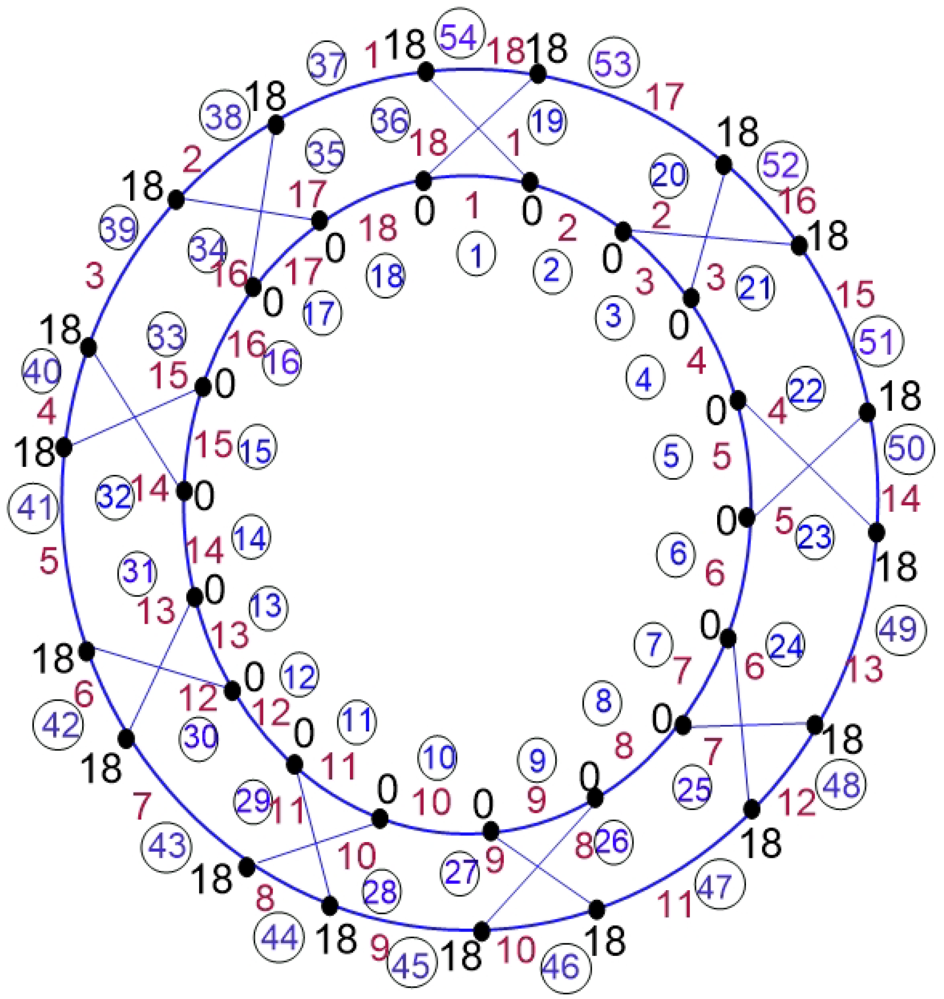
2. Edge-Irregular Reflexive Strength of Cross Prism

A $\nu$-cross prism, commonly referred to as a cross-prism graph, is generated by combining two cycle graphs, $C_{\nu }$, with more edges relating the two identical vertices.

$$\{{\sigma }_{\delta }{\varpi }_{\delta +1},{\sigma }_{\nu }{\varpi }_1\mid 2\le \delta \le (\nu -1),\delta \equiv 0(mod2)\}$$

and

$$\{{\sigma }_{\delta }{\varpi }_{\delta -1},{\sigma }_1{\varpi }_{\nu }\mid 3\le \delta \le (\nu -1),\delta \equiv 1(mod2)\},$$

where $\nu$ is a positive even integer. The cross-prism graph is denoted by $C{P}_{\nu }$ and is illustrated in Figure 1. The $\nu$-cross-prism graph consists of $2\nu$ vertices and $3\nu$ edges.

Theorem 1 describes the edge-irregular reflexive strength of the $C{P}_{\nu }$ graph.

Theorem 1. 

For $\nu >4$, the reflexive edge strength of the cross-prism graph $C{P}_{\nu }$ is given by

$$res(C{P}_{\nu })=\nu$$

Proof. 

The cross-prism graph $C{P}_{\nu }$ has $3\nu$ edges, and for an even $\nu$, $3\nu \equiv 0(mod6)$. Considering Lemma 1, we establish that $\mathrm{res}(C{P}_{\nu })\ge \nu$. To demonstrate the reverse inequality, use the vertex set $V(\check{G_{\nu }})$ and edge set $E(\check{G_{\nu }})$ of the cross-prism graph, as illustrated below, and determine its edge-irregular reflexive strength.

$$V(C{P}_{\nu })=\{{\sigma }_{\delta },{\varpi }_{\delta }|\mathrm{where}1\le \delta \le n\}$$

$$E(C{P}_{\nu })=\{{\sigma }_{\delta }{\sigma }_{\delta +1},{\sigma }_1{\sigma }_{\nu }|1\le i\le (\nu -1)\}$$

$$\cup \{{\varpi }_{\delta }{\varpi }_{\delta +1},{\varpi }_1{\varpi }_{\nu }|1\le \delta \le (\nu -1)\}$$

$$\cup \{{\sigma }_{\delta }{\varpi }_{\delta +1},{\sigma }_n{\varpi }_1|2\le \delta \le (\nu -1)\mid \delta \equiv 0(\mathrm{mod}2)\}$$

$$\cup \{{\sigma }_{\delta }{\varpi }_{\delta -1},{\sigma }_1{\varpi }_{\nu }|3\le \delta \le (\nu -1)\mid \delta \equiv 1(\mathrm{mod}2)\}.$$

For $\nu \ge 4$, the edge-irregular reflexive labeling of $C{P}_{\nu }$ can possibly be defined as follows:

$$\begin{array}{ccc}\hfill {\rm Y}({\sigma }_{\delta })& =& 0,1\le \delta \le \nu .\hfill \\ \hfill {\rm Y}({\varpi }_{\delta })& =& \nu ,1\le \delta \le \nu .\hfill \\ \hfill {\rm Y}({\sigma }_{\delta }{\sigma }_{\delta +1})& =& 1+\delta ,1\le \delta \le (\nu -1).\hfill \\ \hfill {\rm Y}({\sigma }_{\nu }{\sigma }_1)& =& 1.\hfill \\ \hfill {\rm Y}({\varpi }_{\delta }{\varpi }_{\delta +1})& =& \nu -\delta ,1\le \delta \le (\nu -1).\hfill \\ \hfill {\rm Y}({\varpi }_{\nu }{\varpi }_1)& =& \nu .\hfill \\ \hfill {\rm Y}({\sigma }_1{\varpi }_{\nu })& =& 1.\hfill \\ \hfill {\rm Y}({\sigma }_{\nu }{\varpi }_1)& =& \nu .\hfill \\ \hfill {\rm Y}({\sigma }_{\delta }{\varpi }_{\delta +1})& =& \delta ,2\le \delta \le \nu -1,\delta \equiv 0(mod2).\hfill \\ \hfill {\rm Y}({\sigma }_{\delta }{\varpi }_{\delta -1})& =& \delta ,3\le \delta \le \nu -1,\delta \equiv 1(mod2).\hfill \end{array}$$

For $\delta =1,2,3,\dots ,\nu -1$, the edge weights of the edges $a_{\delta }{a}_{\delta +1}$ in $C{P}_{\nu }$ under the labeling ${\rm Y}$ are computed as follows:

$$\begin{array}{ccc}\hfill wt({\sigma }_{\delta }{\sigma }_{\delta +1})& =& {{\rm Y}}_v({\sigma }_{\delta })+{{\rm Y}}_e({\sigma }_{\delta }{\sigma }_{\delta +1})+{{\rm Y}}_v({\sigma }_{\delta +1})\hfill \\ \hfill wt({\sigma }_{\delta }{\sigma }_{\delta +1})& =& 0+\delta +1+0\hfill \\ \hfill wt({\sigma }_{\delta }{\sigma }_{\delta +1})& =& \delta +1.\hfill \end{array}$$

And

$$\begin{array}{ccc}\hfill wt({\sigma }_{\nu }{\sigma }_1)& =& {{\rm Y}}_v({\sigma }_{\nu })+{{\rm Y}}_e({\sigma }_{\nu }{\sigma }_1)+{{\rm Y}}_v({\sigma }_1)\hfill \\ \hfill wt({\sigma }_{\nu }{\sigma }_1)& =& 0+1+0\hfill \\ \hfill wt({\sigma }_{\nu }{\sigma }_1)& =& 1.\hfill \end{array}$$

For $\{2\le \delta \le \nu -1,\mid \delta \equiv 0(mod2)\}$, the edge weights of the edges ${\sigma }_{\delta }{\varpi }_{\delta +1}$ of $C{P}_{\nu }$ under the labeling ${\rm Y}$ are computed as follows:

$$\begin{array}{ccc}\hfill wt({\sigma }_{\delta }{\varpi }_{\delta +1})& =& {{\rm Y}}_v({\sigma }_{\delta })+{{\rm Y}}_e({\sigma }_{\delta }{\varpi }_{\delta +1})+{{\rm Y}}_v({\varpi }_{\delta +1})\hfill \\ \hfill wt({\sigma }_{\delta }{\varpi }_{\delta +1})& =& 0+\delta +\nu \hfill \\ \hfill wt({\sigma }_{\delta }{b}_{\delta +1})& =& \nu +\delta .\hfill \end{array}$$

For $\{3\le \delta \le \nu -1,\mid \delta \equiv 1(mod2)\}$, the edge weights of the edges $a_{\delta }{\varpi }_{\delta -1}$ of $C{P}_{\nu }$ under the labeling ${\rm Y}$ are calculated as follows:

$$\begin{array}{ccc}\hfill wt({\sigma }_{\delta }{\varpi }_{\delta -1})& =& {{\rm Y}}_v({\sigma }_{\delta })+{{\rm Y}}_e({\sigma }_{\delta }{\varpi }_{\delta -1})+{{\rm Y}}_v({\varpi }_{\delta -1})\hfill \\ \hfill wt({\sigma }_{\delta }{\varpi }_{\delta -1})& =& 0+\delta +\nu \hfill \\ \hfill wt({\sigma }_{\delta }{\varpi }_{\delta -1})& =& \nu +\delta .\hfill \end{array}$$

And

$$\begin{array}{ccc}\hfill wt({\sigma }_{\nu }{\varpi }_1)& =& {{\rm Y}}_v({\sigma }_{\nu })+{{\rm Y}}_e({\sigma }_{\nu }{b}_1)+{{\rm Y}}_v({\varpi }_1)\hfill \\ \hfill wt({\sigma }_{\nu }{\varpi }_1)& =& 2\nu .\hfill \\ \hfill wt({\sigma }_1{\varpi }_{\nu })& =& {{\rm Y}}_v({\sigma }_1)+{{\rm Y}}_e({\sigma }_1{\varpi }_{\nu })+{{\rm Y}}_v({\varpi }_{\nu })\hfill \\ \hfill wt({\sigma }_1{\varpi }_{\nu })& =& \nu +1.\hfill \end{array}$$

For $\delta =1,2,3\dots ,\nu -1$, the edge weights of the edges ${\varpi }_{\delta }{\varpi }_{\delta +1}$ are

$$\begin{array}{ccc}\hfill wt({\varpi }_{\delta }{\varpi }_{\delta +1})& =& {{\rm Y}}_v({\varpi }_{\delta })+{{\rm Y}}_e({\varpi }_{\delta }{\varpi }_{\delta +1})+{{\rm Y}}_v({\varpi }_{\delta +1})\hfill \\ \hfill wt({\varpi }_{\delta }{\varpi }_{\delta +1})& =& \nu +\nu -\delta +\nu \hfill \\ \hfill wt({\varpi }_{\delta }{\varpi }_{\delta +1})& =& 3\nu -\delta .\hfill \end{array}$$

And

$$\begin{array}{ccc}\hfill wt({\varpi }_{\nu }{\varpi }_1)& =& {\varpi }_v({\varpi }_{\nu })+{\varpi }_e({\varpi }_{\nu }{\varpi }_1)+{{\rm Y}}_v({\varpi }_1)\hfill \\ \hfill wt({\varpi }_{\nu }{\varpi }_1)& =& 3\nu .\hfill \end{array}$$

This labeling is explained by Figure 2 with the weights of the corresponding edges.

Figure 2. Edge-irregular reflexive labeling of $C{P}_{18}$.

Figure 2. Edge-irregular reflexive labeling of $C{P}_{18}$.

From the calculations of the weights of the edges of $C{P}_{\nu }$, we can easily see that the weights of different edges are distinct, which proves that ${\rm Y}$ is an edge-irregular reflexive labeling and therefore $res(C{P}_{\nu })\le \nu .$ Hence, the theorem is proved. □

3. Duplication of Graph

Vaidya and Barasara indicated vertex-edge duplication in [13], whereas Vaidya and Dani analyzed edge-vertex duplication in [14]. These notions are clarified as follows.

Definition 1 

([14]).

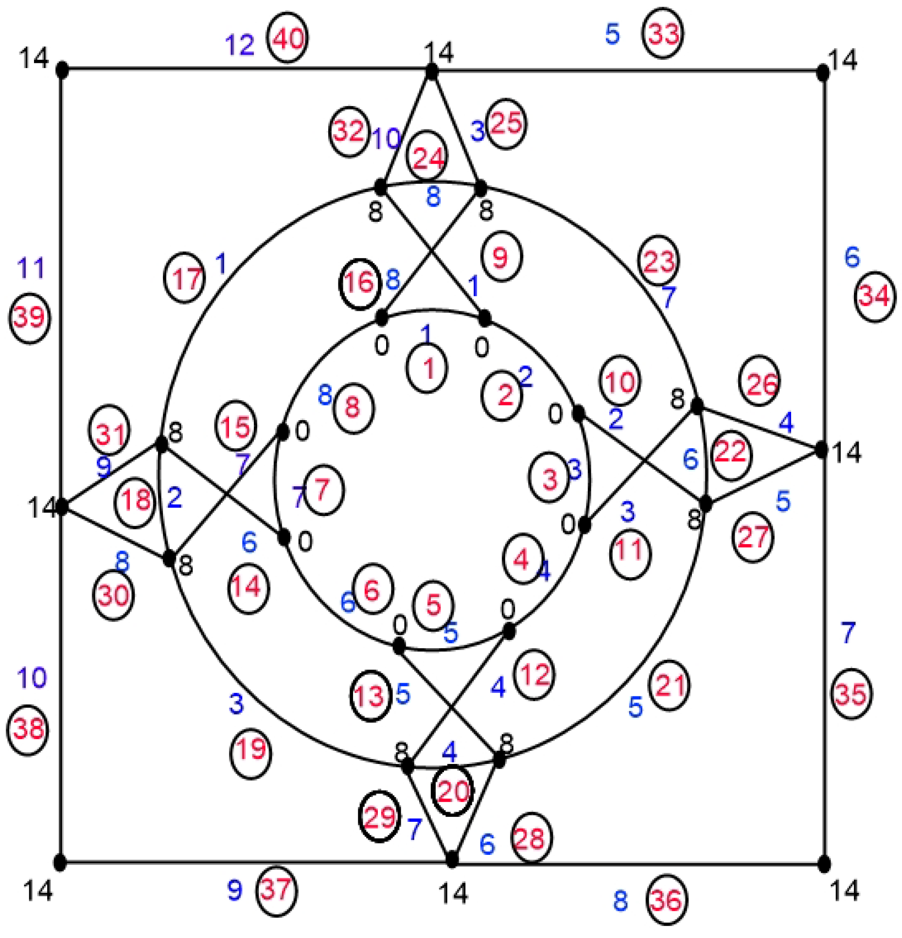
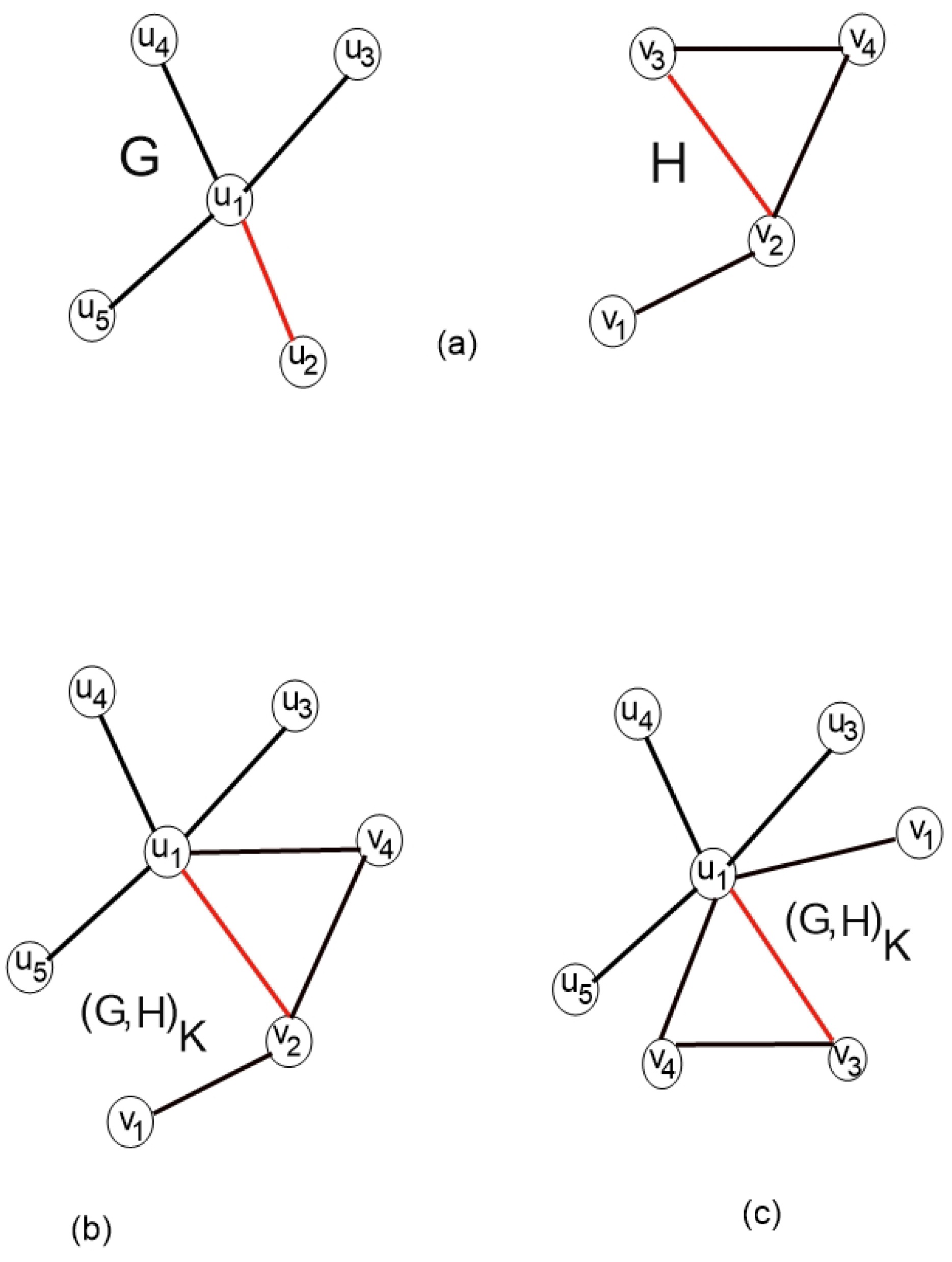
• In a graph S, establishing a new vertex u using $N(u)=N(\varsigma )$ produces a new graph $S^{\prime }$. This is known as the duplication of the vertex ς.
  Vertex duplication by an edge $p=v_j{w}_j$ in a graph S provides a new graph $S^{\prime }$ with $N(v_j)=\{{\varkappa }_j,w_j\}$ and $N(w_j)=\{{\varkappa }_j,v_j\}$. Figure 3 depicts an example of edge-induced vertex duplication in $C_3$.
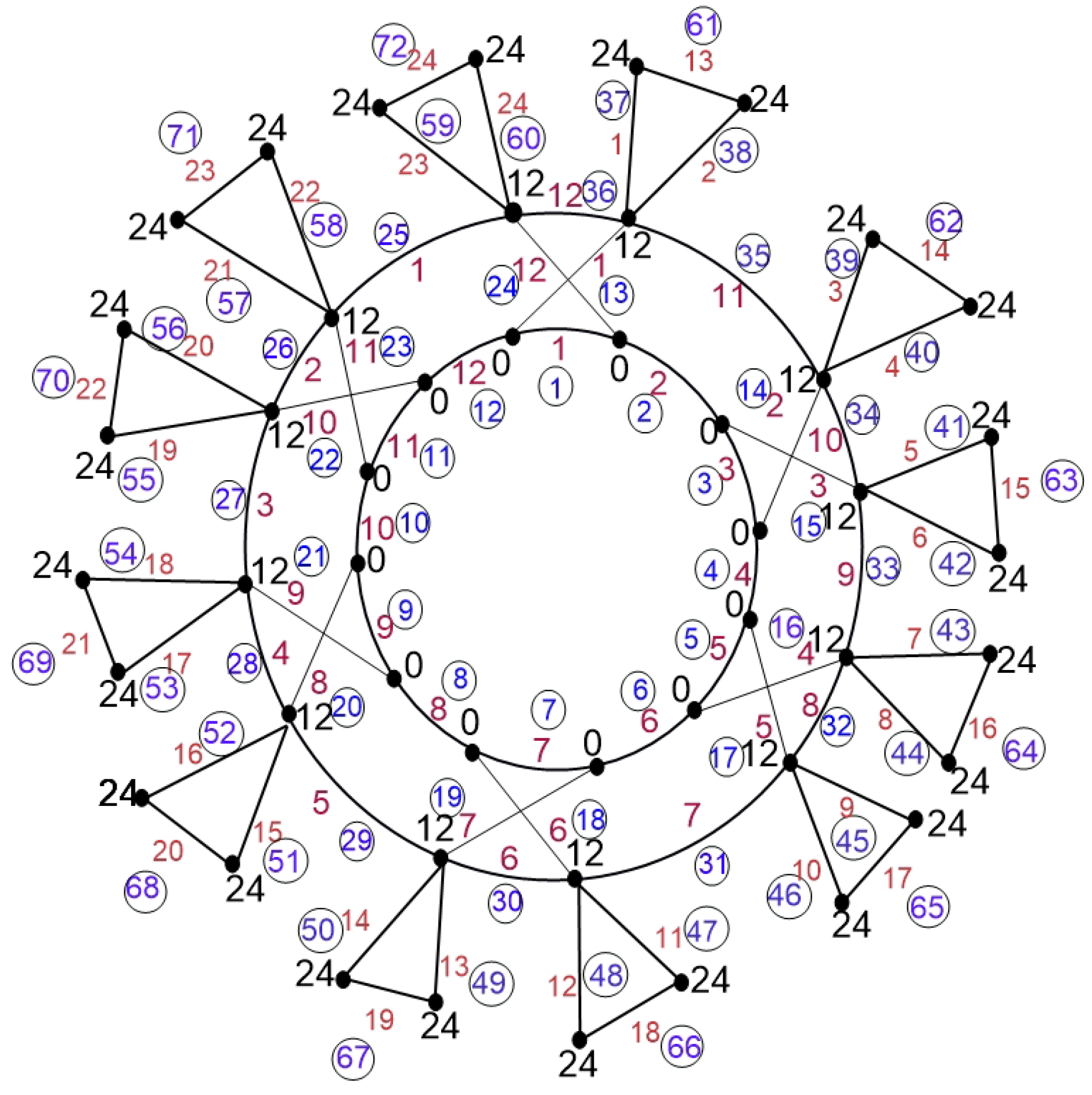
• When a vertex ς replicates an edge $e={\varsigma }_{\delta }{\varsigma }_{\delta +1}$ in a graph S, a corresponding graph $S^{\prime }$ is produced with $N(\varsigma )=\{{\varsigma }_{\delta },{\varsigma }_{\delta +1}\}$.
  Let $C{P}_{\nu }^{\prime }$ be the graph acquired from $C{P}_{\nu }$ by duplication of each vertex ${\varpi }_i$ by an edge. This graph has $4\nu$ vertices and $6\nu$ edges. Then, the next Theorem 2 describes the edge-irregular reflexive strength of $C{P}_{\nu }^{\prime }$.

Theorem 2. 

For even $\nu \ge 4$ and ν, the edge-irregular reflexive strength of ${\mathit{CP}}_{\nu }^{\prime }$ is given by

$$res(C{P}_{\nu }^{\prime })=2\nu .$$

Proof. 

Since the number of edges of $C{P}_{\nu }^{\prime }$ is $6\nu$, where $\nu$ is even, we have $6\nu \equiv 0(\mathrm{mod}6)$. Therefore, by Lemma 1, we have $res(C{P}_{\nu })\ge 2\nu$. To prove the reverse inequality, we assume $\check{G_{\nu }}\cong C{P}_{\nu }^{\prime }$ and that the vertex set $V(\check{G_{\nu }})$ and edge set $E(\check{G_{\nu }})$ of $\check{G_{\nu }}$ are as given below:

$$V(C{P}_{\nu }^{\prime })=\{{\sigma }_{\delta },{\varpi }_{\delta }|1\le \delta \le \nu \}\cup \{c_{\delta }|1\le \delta \le 2\nu \},$$

$$E(C{P}_{\nu }^{\prime })=\{{\sigma }_{\delta }{\sigma }_{\delta +1},{\sigma }_1{\sigma }_{\nu }|1\le \delta \le (\nu -1)\}$$

$$\cup \{{\varpi }_{\delta }{\varpi }_{\delta +1},{\varpi }_1{\varpi }_{\nu }|1\le \delta \le (\nu -1)\}$$

$$\cup \left\{{\sigma }_{\delta }{\varpi }_{\delta +1},{\sigma }_{\nu }{\varpi }_1|2\le \delta \le (\nu -1),\delta \equiv 0(\mathrm{mod}2)\right\}$$

$$\cup \left\{{\sigma }_{\delta }{\varpi }_{\delta -1},{\sigma }_1{\varpi }_{\nu }|3\le \delta \le (\nu -1),\delta \equiv 1(\mathrm{mod}2)\right\}$$

$$\cup \{c_{2\delta +1},c_{2\delta +2}|0\le \delta \le \nu \}$$

$$\cup \{c_{\delta }{\varpi }_{\lfloor {\displaystyle \frac{\delta +1}{2}}\rfloor },c_1{\varpi }_1|1\le \delta \le 2\nu \}.$$

For $\nu \ge 4$, we define the edge-irregular reflexive labeling of $C{P}_{\nu }^{\prime }$ in the following way:

$$\begin{array}{ccc}\hfill {\rm Y}({\sigma }_{\delta })& =& 0,1\le \delta \le \nu .\hfill \\ \hfill {\rm Y}({\varpi }_{\delta })& =& \nu ,1\le \delta \le \nu .\hfill \\ \hfill {\rm Y}(c_{\delta })& =& k,1\le \delta \le \nu .\hfill \\ \hfill {\rm Y}({\sigma }_{\delta }{\sigma }_{\delta +1})& =& 1+\delta ,1\le \delta \le (\nu -1).\hfill \\ \hfill {\rm Y}({\sigma }_{\nu }{\sigma }_1)& =& 1,\hfill \\ \hfill {\rm Y}({\varpi }_{\delta }{\varpi }_{\delta +1})& =& \nu -\delta ,1\le \delta \le (\nu -1).\hfill \\ \hfill {\rm Y}({\varpi }_{\nu }{\varpi }_1)& =& \nu ,\hfill \\ \hfill {\rm Y}({\sigma }_1{\varpi }_{\nu })& =& 1,\hfill \\ \hfill {\rm Y}({\sigma }_{\nu }{\varpi }_1)& =& \nu ,\hfill \\ \hfill {\rm Y}({\sigma }_{\delta }{\varpi }_{\delta +1})& =& \delta ,2\le \delta \le \nu -1,\delta \equiv 0(\mathrm{mod}2).\hfill \\ \hfill {\rm Y}({\sigma }_{\delta }{\varpi }_{\delta -1})& =& \delta ,3\le \delta \le \nu -1,\delta \equiv 1(\mathrm{mod}2).\hfill \\ \hfill {\rm Y}(c_{2\delta +1}{c}_{2\delta +2})& =& \nu +\delta +1,0\le \delta \le \kappa .\hfill \\ \hfill {\rm Y}(c_{\delta }{\varpi }_{\lfloor {\displaystyle \frac{\delta +1}{2}}\rfloor })& =& \delta ,1\le \delta \le \kappa .\hfill \\ \hfill {\rm Y}(c_1{\varpi }_1)& =& 1.\hfill \end{array}$$

For $\delta =1,2,3\dots ,\nu -1$, the edge weights of the edges $a_{\delta }{\sigma }_{\delta +1}$ in $C{P}_{\nu }^{\prime }$ under the labeling ${\rm Y}$ are the following:

$$\begin{array}{ccc}\hfill wt({\sigma }_{\delta }{\sigma }_{\delta +1})& =& {{\rm Y}}_v({\sigma }_{\delta })+{{\rm Y}}_e({\sigma }_{\delta }{\sigma }_{\delta +1})+{{\rm Y}}_v({\sigma }_{\delta +1})\hfill \\ \hfill wt({\sigma }_{\delta }{\sigma }_{\delta +1})& =& 0+\delta +1+0\hfill \\ \hfill wt({\sigma }_{\delta }{\sigma }_{\delta +1})& =& \delta +1.\hfill \end{array}$$

And

$$\begin{array}{ccc}\hfill wt({\sigma }_{\nu }{\sigma }_1)& =& {{\rm Y}}_v({\sigma }_{\nu })+{{\rm Y}}_e({\sigma }_{\nu }{\sigma }_1)+{{\rm Y}}_v({\sigma }_1)\hfill \\ \hfill wt({\sigma }_{\nu }{\sigma }_1)& =& 0+1+0\hfill \\ \hfill wt({\sigma }_{\nu }{\sigma }_1)& =& 1..\hfill \end{array}$$

For $2\le \delta \le \nu -1,\mid \delta \equiv 0(mod2)$, the edge weights of the edges ${\sigma }_{\delta }{\varpi }_{\delta +1}$ in $C{P}_{\nu }^{\prime }$ under the labeling ${\rm Y}$ are the following;

$$\begin{array}{ccc}\hfill wt({\sigma }_{\delta }{\varpi }_{\delta +1})& =& {{\rm Y}}_v({\sigma }_{\delta })+{{\rm Y}}_e({\sigma }_{\delta }{\varpi }_{\delta +1})+{{\rm Y}}_v({\varpi }_{\delta +1})\hfill \\ \hfill wt({\sigma }_{\delta }{\varpi }_{\delta +1})& =& 0+\delta +\nu \hfill \\ \hfill wt({\sigma }_{\delta }{\varpi }_{\delta +1})& =& \nu +\delta .\hfill \end{array}$$

For $3\le \delta \le \nu -1,\delta \equiv 1(\mathrm{mod}2)$, the edge weights of the edges ${\sigma }_{\delta }{\varpi }_{\delta -1}$ in $C{P}_{\nu }^{\prime }$ under the labeling ${\rm Y}$ are the following:

$$\begin{array}{ccc}\hfill wt({\sigma }_{\delta }{\varpi }_{\delta -1})& =& {{\rm Y}}_v({\sigma }_{\delta })+{{\rm Y}}_e({\sigma }_{\delta }{\varpi }_{\delta -1})+{{\rm Y}}_v({\varpi }_{\delta -1})\hfill \\ \hfill wt({\sigma }_{\delta }{\varpi }_{\delta -1})& =& 0+\delta +\nu \hfill \\ \hfill wt({\sigma }_{\delta }{\varpi }_{\delta -1})& =& \nu +\delta .\hfill \end{array}$$

And,

$$\begin{array}{ccc}\hfill wt({\sigma }_{\nu }{\varpi }_1)& =& {{\rm Y}}_v({\sigma }_{\nu })+{{\rm Y}}_e({\sigma }_{\nu }{\varpi }_1)+{{\rm Y}}_v({\varpi }_1)\hfill \\ \hfill wt({\sigma }_{\nu }{\varpi }_1)& =& 2\nu .\hfill \\ \hfill wt({\sigma }_1{\varpi }_{\nu })& =& {{\rm Y}}_v({\sigma }_1)+{{\rm Y}}_e({\sigma }_1{\varpi }_{\nu })+{{\rm Y}}_v({\varpi }_{\nu })\hfill \\ \hfill wt({\sigma }_1{\varpi }_{\nu })& =& \nu +1.\hfill \end{array}$$

For $\delta =1,2,\dots ,\nu -1$, the edge weights of the edges ${\varpi }_{\delta }{\varpi }_{\delta +1}$ in $C{P}_{\nu }^{\prime }$ are

$$\begin{array}{ccc}\hfill wt({\varpi }_{\delta }{\varpi }_{\delta +1})& =& f_v({\varpi }_{\delta })+{{\rm Y}}_e({\varpi }_{\delta }{\varpi }_{\delta +1})+{{\rm Y}}_v({\varpi }_{\delta +1})\hfill \\ \hfill wt({\varpi }_{\delta }{\varpi }_{\delta +1})& =& \nu +\nu -\delta +\nu \hfill \\ \hfill wt({\varpi }_{\delta }{\varpi }_{\delta +1})& =& 3\nu -\delta .\hfill \end{array}$$

And

$$\begin{array}{ccc}\hfill wt({\varpi }_{\nu }{\varpi }_1)& =& {{\rm Y}}_v({\varpi }_{\nu })+{{\rm Y}}_e({\varpi }_{\nu }{\varpi }_1)+{{\rm Y}}_v({\varpi }_1)\hfill \\ \hfill wt({\varpi }_{\nu }{\varpi }_1)& =& 3\nu .\hfill \end{array}$$

For $\delta =1,2,\dots ,2\nu$, the edge weights of the edges $c_{2\delta +1}{c}_{2\delta +2}$ and $c_{\delta }{\varpi }_{\lfloor {\displaystyle \frac{\delta +1}{2}}\rfloor }$ in $C{P}_{\nu }^{\prime }$ under the labeling ${\rm Y}$ are given by

$$\begin{array}{ccc}\hfill wt(c_{2\delta +1}{c}_{2\delta +2})& =& 5\nu +\delta +1,0\le \delta \le \nu -1.\hfill \\ \hfill wt(c_{\delta }{\varpi }_{\lfloor {\displaystyle \frac{\delta +1}{2}}\rfloor })& =& 3\nu +\delta ,1\le \delta \le 2\nu .\hfill \end{array}$$

This labeling is explained by Figure 4 with the weights of the corresponding edges.

Figure 4. Edge-irregular reflexive labeling of $C{P}_{12}^{\prime }$.

Figure 4. Edge-irregular reflexive labeling of $C{P}_{12}^{\prime }$.

From the calculations of the weights of the edges of $C{P}_{\nu }^{\prime }$, we easily see that the weights of different edges are distinct, which proves that ${\rm Y}$ is an edge-irregular reflexive labeling and therefore $res(C{P}_{\nu }^{\prime })\le 2\nu .$ Hence, the theorem is proved. □

4. ${\mathit{HACP}}_{\mathit{\nu }}$ Graphs

The graph $HAC{P}_{\nu }$ consists of $3\nu$ vertices and $5\nu$ edges. The vertices and edge sets are defined as

$$V(HAC{P}_{\nu })=\{{\sigma }_{\delta },{\varpi }_{\delta },c_{\delta }\}, \mathrm{where}1\le \delta \le \nu .$$

$$\begin{array}{ccc}\hfill E(HAC{P}_{\nu })& =& \{{\sigma }_{\delta }{\sigma }_{\delta +1},{\sigma }_1{\sigma }_{\nu }|1\le \delta \le \nu -1\}\hfill \\ & \cup & \{{\varpi }_{\delta }{\varpi }_{\delta +1},{\varpi }_1{\varpi }_{\nu }|1\le \delta \le \nu -1\}\hfill \\ & \cup & \{{\sigma }_{\delta }{\varpi }_{\delta +1},{\sigma }_{\nu }{\varpi }_1|2\le \delta \le \nu -1,\delta \equiv 0(\mathrm{mod}2)\}\hfill \\ & \cup & \{{\sigma }_{\delta }{\varpi }_{\delta -1},{\sigma }_1{\varpi }_{\nu }|3\le \delta \le \nu -1,\delta \equiv 1(\mathrm{mod}2)\}\hfill \\ & \cup & \{c_{\delta }{c}_{\delta +1},c_{\nu }{c}_1|0\le \delta \le \nu \}\hfill \\ & \cup & \{c_{\delta }{\varpi }_{\delta -1},c_1{\varpi }_{\nu }|3\le \delta \le \nu -1,\delta \equiv 1(\mathrm{mod}2)\}\hfill \\ & \cup & \{c_{\delta }{\varpi }_{\delta }|1\le \delta \le \nu -1,\delta \equiv 1(\mathrm{mod}2)\}.\hfill \end{array}$$

The graph of $(HAC{P}_{\nu })$ is shown in Figure 5.

Theorem 3. 

For $\nu \ge 4$, the edge-irregular reflexive labeling of $(HAC{P}_{\nu })$ graph is

$$res(HAC{P}_{\nu })=\left\{\begin{array}{cc}\lceil {\displaystyle \frac{5\nu }{3}}\rceil ,\hfill & \mathit{if}5\nu \not\equiv 2,3(mod6)\hfill \\ \lceil {\displaystyle \frac{5\nu }{3}}\rceil +1,\hfill & \mathit{if}5\nu \equiv 2,3(mod6)\hfill \end{array}\right.$$

Proof. 

Since the $|E(HAC{P}_{\nu })|=5\nu$, by Lemma 1, we find that

$$res(HAC{P}_{\nu })\ge \left\{\begin{array}{cc}\lceil {\displaystyle \frac{5\nu }{3}}\rceil ,\hfill & \mathrm{if}5\nu \not\equiv 2,3(\mathrm{mod}6)\hfill \\ \lceil {\displaystyle \frac{5\nu }{3}}\rceil +1,\hfill & \mathrm{if}5\nu \equiv 2,3(\mathrm{mod}6)\hfill \end{array}\right.$$

For the converse of the above inequality, we will define the edge-irregular reflexive labeling of $HAC{P}_{\nu }$ for $\nu \ge 4$, in the following way:

$$k=\left\{\begin{array}{cc}\lceil {\displaystyle \frac{5\nu }{3}}\rceil ,\hfill & \mathrm{if}5\nu \not\equiv 2,3(\mathrm{mod}6)\hfill \\ \lceil {\displaystyle \frac{5\nu }{3}}\rceil +1,\hfill & \mathrm{if}5\nu \equiv 2,3(\mathrm{mod}6)\hfill \end{array}\right.$$

then, the vertices of $HAC{P}_{\nu }$ are labeled as

$$\begin{array}{ccc}\hfill {\rm Y}({\sigma }_{\delta })& =& 0,1\le \delta \le \nu .\hfill \\ \hfill {\rm Y}({\varpi }_{\delta })& =& \nu ,1\le \delta \le \nu .\hfill \\ \hfill {\rm Y}(c_{\delta })& =& \kappa ,1\le \delta \le \nu .\hfill \\ \hfill {\rm Y}({\sigma }_{\delta }{\sigma }_{\delta +1})& =& 1+\delta ,1\le \delta \le (\nu -1).\hfill \\ \hfill {\rm Y}({\sigma }_{\nu }{\sigma }_1)& =& 1,\hfill \\ \hfill {\rm Y}({\varpi }_{\delta }{\varpi }_{\delta +1})& =& \nu -\delta ,1\le \delta \le (\nu -1).\hfill \\ \hfill {\rm Y}({\varpi }_{\nu }{\varpi }_1)& =& \nu ,\hfill \\ \hfill {\rm Y}({\sigma }_1{\varpi }_{\nu })& =& 1,\hfill \\ \hfill {\rm Y}({\sigma }_{\nu }{\varpi }_1)& =& \nu ,\hfill \\ \hfill {\rm Y}({\sigma }_{\delta }{\varpi }_{\delta +1})& =& \delta ,\{1\le \delta \le (\nu -1)\mid \delta \equiv 0(\mathrm{mod}2)\}.\hfill \\ \hfill {\rm Y}({\sigma }_{\delta }{\varpi }_{\delta -1})& =& \delta ,\{1\le \delta \le (\nu -1)\mid \delta \equiv 1(\mathrm{mod}2)\}.\hfill \\ \hfill {\rm Y}(c_{\delta }{c}_{\delta +1})& =& 4\lfloor {\displaystyle \frac{\nu }{6}}\rfloor +\delta ,1\le \delta \le (\nu -1).\hfill \\ \hfill {\rm Y}(c_{\nu }{c}_1)& =& 4\lfloor {\displaystyle \frac{\nu }{6}}\rfloor +\nu .\hfill \\ \hfill {\rm Y}(c_{\delta }{\varpi }_{\delta -1})& =& 2\lfloor {\displaystyle \frac{\nu }{6}}\rfloor +\delta -1,\{3\le \delta \le (\nu -1)\mid \delta \equiv 1(\mathrm{mod}2)\}.\hfill \\ \hfill {\rm Y}(c_{\delta }{\varpi }_{\delta })& =& 2\lfloor {\displaystyle \frac{\nu }{6}}\rfloor +\delta ,\{1\le \delta \le (\nu -1)\mid \delta \equiv 1(\mathrm{mod}2)\}.\hfill \\ \hfill {\rm Y}(c_1{\varpi }_{\nu })& =& 2\lfloor {\displaystyle \frac{\nu }{6}}\rfloor +\nu .\hfill \end{array}$$

This labeling is explained in Figure 6.

Figure 6. Edge-irregular reflexive labeling of $HAC{P}_8$.

Figure 6. Edge-irregular reflexive labeling of $HAC{P}_8$.

For $\delta =1,2,3,\dots ,\nu -1$, the edge weights of the edges ${\sigma }_{\delta }{\sigma }_{\delta +1}$ in $HAC{P}_{\nu }$ under the labeling ${\rm Y}$ are the following:

$$\begin{array}{ccc}\hfill wt({\sigma }_{\delta }{\sigma }_{\delta +1})& =& {{\rm Y}}_v({\sigma }_{\delta })+{{\rm Y}}_e({\sigma }_{\delta }{\sigma }_{\delta +1})+{{\rm Y}}_v({\sigma }_{\delta +1})\hfill \\ \hfill wt({\sigma }_{\delta }{\sigma }_{\delta +1})& =& \delta +1.\hfill \end{array}$$

And

$$\begin{array}{ccc}\hfill wt({\sigma }_{\nu }{\sigma }_1)& =& {{\rm Y}}_v({\sigma }_{\nu })+{{\rm Y}}_e({\sigma }_{\nu }{\sigma }_1)+{{\rm Y}}_v({\sigma }_1)=1.\hfill \end{array}$$

For $\{2\le \delta \le (\nu -1)\mid \delta \equiv 0(mod2)\}$, the edge weights of the edges ${\sigma }_{\delta }{b}_{\delta +1}$ in $HAC{P}_{\nu }$ under the labeling ${\rm Y}$ are the following:

$$\begin{array}{ccc}\hfill wt({\sigma }_{\delta }{\varpi }_{\delta +1})& =& {{\rm Y}}_v({\sigma }_{\delta })+{{\rm Y}}_e({\sigma }_{\delta }{\varpi }_{\delta +1})+{{\rm Y}}_v({\varpi }_{\delta +1})\hfill \\ \hfill wt({\sigma }_{\delta }{\varpi }_{\delta +1})& =& \nu +\delta .\hfill \end{array}$$

For $\{3\le \delta \le (\nu -1)\mid \delta \equiv 1(mod2)\}$, the edge weights of the edges ${\sigma }_{\delta }{\varpi }_{\delta -1}$ in $HAC{P}_{\nu }$ under the labeling ${\rm Y}$ are the following:

$$\begin{array}{ccc}\hfill wt({\sigma }_{\delta }{\varpi }_{\delta -1})& =& {{\rm Y}}_v({\sigma }_{\delta })+{{\rm Y}}_e({\sigma }_{\delta }{\varpi }_{\delta -1})+{{\rm Y}}_v({\varpi }_{\delta -1})\hfill \\ \hfill wt({\sigma }_{\delta }{\varpi }_{\delta -1})& =& \nu +\delta .\hfill \end{array}$$

And

$$\begin{array}{ccc}\hfill wt({\sigma }_{\nu }{\varpi }_1)& =& {{\rm Y}}_v({\sigma }_{\nu })+{{\rm Y}}_e({\sigma }_{\nu }{\varpi }_1)+{{\rm Y}}_v({\varpi }_1)\hfill \\ \hfill wt({\sigma }_{\nu }{\varpi }_1)& =& 0+\nu +\nu \hfill \\ \hfill wt({\sigma }_{\nu }{\varpi }_1)& =& 2\nu .\hfill \\ \hfill wt({\sigma }_1{\varpi }_{\nu })& =& {{\rm Y}}_v({\sigma }_1)+{{\rm Y}}_e({\sigma }_1{\varpi }_{\nu })+{{\rm Y}}_v({\varpi }_{\nu })\hfill \\ \hfill wt({\sigma }_1{\varpi }_{\nu })& =& 0+1+\nu \hfill \\ \hfill wt({\sigma }_1{\varpi }_n)& =& \nu +1.\hfill \end{array}$$

For $\delta =1,2,\dots ,\nu -1$, the edge weights of the edges ${\varpi }_{\delta }{\varpi }_{\delta +1}$ in $HAC{P}_{\nu }$ under the labeling ${\rm Y}$ are the following:

$$\begin{array}{ccc}\hfill wt({\varpi }_{\delta }{\varpi }_{\delta +1})& =& {{\rm Y}}_v({\varpi }_{\delta })+{{\rm Y}}_e({\varpi }_{\delta }{\varpi }_{\delta +1})+{{\rm Y}}_v({\varpi }_{\delta +1})\hfill \\ \hfill wt({\varpi }_{\delta }{\varpi }_{\delta +1})& =& 3\nu -\delta .\hfill \end{array}$$

And

$$\begin{array}{ccc}\hfill wt({\varpi }_{\nu }{\varpi }_1)& =& {{\rm Y}}_v({\varpi }_{\nu })+{{\rm Y}}_e({\varpi }_{\nu }{\varpi }_1)+{{\rm Y}}_v({\varpi }_1)=3\nu \hfill \end{array}$$

For $\delta =1,2,\dots ,\nu -1$, the edge weights of the edges $(c_{\delta }{c}_{\delta +1})$ and $(c_{\delta }{\varpi }_{\delta -1})$ in $HAC{P}_{\nu }$ under the labeling ${\rm Y}$ are the following:

$$\begin{array}{ccc}\hfill wt(c_{\delta }{c}_{\delta +1})& =& 4\nu +\delta ,1\le \delta \le (\nu -1).\hfill \\ \hfill wt(c_{\delta }{\varpi }_{\delta -1})& =& 3\nu +\delta -1,\{3\le \delta \le (\nu -1)\mathrm{and}\delta \equiv 1(\mathrm{mod}2)\}.\hfill \\ \hfill wt(c_{\delta }{\varpi }_{\delta })& =& 3\nu +\delta ,\{1\le \delta \le (\nu -1)\mathrm{and}\delta \equiv 1(\mathrm{mod}2)\}.\hfill \\ \hfill wt(c_1{\varpi }_{\nu })& =& 4\nu ,\hfill \\ \hfill wt(c_{\nu }{c}_1)& =& 5\nu .\hfill \end{array}$$

From the above computations of the weights of edges, it is very easy to see that the weights of any pair of different edges are distinct. Thus, ${\rm Y}$ is an edge-irregular reflexive labeling and therefore,

$$res(HAC{P}_{\nu })\le \left\{\begin{array}{cc}\lceil {\displaystyle \frac{5\nu }{3}}\rceil ,\hfill & \mathrm{if}5\nu \not\equiv 2,3(\mathrm{mod}6)\hfill \\ \lceil {\displaystyle \frac{5\nu }{3}}\rceil +1,\hfill & \mathrm{if}5\nu \equiv 2,3(\mathrm{mod}6)\hfill \end{array}\right\}.$$

□

5. Glowing Graph ${({\mathit{C}\mathit{P}}_{\mathit{\nu }},{\mathit{D}}_{\mathit{\nu }})}_{{\mathit{C}}_{\mathit{\nu }}}$

Assume $\check{G_{\nu }}$ and H are two graphs. ${(\check{G_{\nu }},H)}_{\kappa }$ illustrates the operation of merging $\check{G_{\nu }}$ and H on a common subgraph $\kappa$. The consequent graph has the following vertex and edge sets:

$$\begin{array}{ccc}\hfill V({(\check{G_{\nu }},H)}_{\kappa })& =& (V(\check{G_{\nu }})-V(\kappa ))\cup (V(H)-V(\kappa ))\cup V(\kappa )\hfill \\ \hfill E({(\check{G_{\nu }},H)}_{\kappa })& =& (E(\check{G_{\nu }})-E(\kappa ))\cup (E(H)-E(\kappa ))\cup E(\kappa )\hfill \end{array}$$

Figure 7a demonstrates how graphs $\check{G_{\nu }}$ and H are linked together via the common subgraph $\kappa$. The common subgraph $\kappa$ is depicted as the red edge-induced subgraph in both graphs, denoted as $G\left[u_1{u}_2\right]$ in G and $H\left[v_2{v}_3\right].$ in H. In $\check{G_{\nu }}$, this corresponds to the edge $u_1{u}_2$, but in H, it is the edge $v_2{v}_3$. Figure 7b,c shows two unique approaches for integrating $\check{G_{\nu }}$ and H using $\kappa$.

Theorem 4. 

For $\nu \ge 4$, the edge-irregular reflexive strength for ${(C{P}_{\nu },D_{\nu })}_{C_{\nu }}$ is given by

$$res{(C{P}_{\nu },D_{\nu })}_{C_{\nu }}=\left\{\begin{array}{cc}\lceil {\displaystyle \frac{5\nu }{3}}\rceil ,\hfill & \mathit{if}5\nu \not\equiv 2,3(mod6)\hfill \\ \lceil {\displaystyle \frac{5\nu }{3}}\rceil +1,\hfill & \mathit{if}5\nu \equiv 2,3(mod6)\hfill \end{array}\right.$$

Proof. 

The vertex set $V({(C{P}_{\nu },D_{\nu })}_{C_{\nu }})$ and edge set $E({(C{P}_{\nu },D_{\nu })}_{C_{\nu }})$ are defined as below:

$$V({(C{P}_{\nu },D_{\nu })}_{C_{\nu }})=\left\{{\sigma }_{\delta }\right\}\cup \left\{{\varpi }_{\delta }\right\}\cup \left\{c_i\right\} \mathrm{where}1\le \delta \le \nu .$$

$$\begin{array}{ccc}\hfill E({(C{P}_{\nu },D_{\nu })}_{C_{\nu }})& =& \{{\sigma }_{\delta }{\sigma }_{\delta +1},{\sigma }_1{\sigma }_{\nu }|1\le \delta \le \nu -1\}\hfill \\ & \cup & \{{\varpi }_{\delta }{\varpi }_{\delta +1},{\varpi }_1{\varpi }_{\nu }|1\le \delta \le \nu -1\}\hfill \\ & \cup & \{{\sigma }_{\delta }{\varpi }_{\delta +1},{\sigma }_{\nu }{\varpi }_1|2\le \delta \le \nu -1,\delta \equiv 0(\mathrm{mod}2)\}\hfill \\ & \cup & \{{\sigma }_{\delta }{\varpi }_{\delta -1},{\sigma }_1{\varpi }_{\nu }|3\le \delta \le \nu -1,\delta \equiv 1(\mathrm{mod}2)\}\hfill \\ & \cup & \{c_1{c}_{\delta +1},c_1{c}_{\nu }|1\le \delta \le \nu -1\}\hfill \\ & \cup & \{{\varpi }_1{c}_{\delta }|1\le \delta \le \nu \}\hfill \end{array}$$

The graph ${(C{P}_{\nu },D_{\nu })}_{C_{\nu }}$ is depicted in Figure 8.

Let $\kappa =\left\{\begin{array}{cc}\lceil {\displaystyle \frac{5\nu }{3}}\rceil ,\hfill & \mathrm{if}5\nu \not\equiv 2,3(\mathrm{mod}6)\hfill \\ \lceil {\displaystyle \frac{5\nu }{3}}\rceil +1,\hfill & \mathrm{if}5\nu \equiv 2,3(\mathrm{mod}6)\hfill \end{array}\right.$

Then, from Lemma 1, we find that $res({(C{P}_{\nu },D_{\nu })}_{C_{\nu }})\ge \kappa$. To prove the reverse inequality to this, we define the edge irregular reflexive labeling of ${(C{P}_{\nu },D_{\nu })}_{C_{\nu }}$ for $\nu \ge 4$, as follows:

$$\begin{array}{ccc}\hfill {\rm Y}({\sigma }_{\delta })& =& 0,1\le \delta \le \nu .\hfill \\ \hfill {\rm Y}({\varpi }_{\delta })& =& \nu ,1\le \delta \le \nu .\hfill \\ \hfill {\rm Y}(c_{\delta })& =& k,1\le \delta \le \nu .\hfill \\ \hfill {\rm Y}({\sigma }_{\delta }{\sigma }_{\delta +1})& =& 1+\delta ,1\le \delta \le (\nu -1).\hfill \\ \hfill {\rm Y}({\sigma }_{\nu }{\sigma }_1)& =& 1.\hfill \\ \hfill {\rm Y}({\varpi }_{\delta }{\varpi }_{\delta +1})& =& \nu -\delta ,1\le \delta \le (\nu -1).\hfill \\ \hfill {\rm Y}({\varpi }_{\nu }{\varpi }_1)& =& \nu .\hfill \\ \hfill {\rm Y}({\sigma }_1{\varpi }_{\nu })& =& 1.\hfill \\ \hfill {\rm Y}({\sigma }_{\nu }{\varpi }_1)& =& \nu .\hfill \\ \hfill {\rm Y}({\sigma }_{\delta }{\varpi }_{\delta +1})& =& \delta ,\{1\le \delta \le (\nu -1),\delta \equiv 0(\mathrm{mod}2)\}.\hfill \\ \hfill {\rm Y}({\sigma }_{\delta }{\varpi }_{\delta -1})& =& \delta ,\{1\le \delta \le (\nu -1),\delta \equiv 1(\mathrm{mod}2)\}.\hfill \\ \hfill {\rm Y}(c_{\delta }{c}_{\delta +1})& =& 4\lfloor {\displaystyle \frac{\nu }{6}}\rfloor +\delta ,1\le \delta \le (\nu -1).\hfill \\ \hfill {\rm Y}(c_{\nu }{c}_1)& =& 4\lfloor {\displaystyle \frac{\nu }{6}}\rfloor +\nu .\hfill \\ \hfill {\rm Y}(c_{\delta }{b}_{\delta })& =& 2\lfloor {\displaystyle \frac{\nu }{6}}\rfloor +\delta ,1\le \delta \le (\nu ).\hfill \end{array}$$

This labeling is explained in Figure 9.

Now, we shall compute the weights of edges for the above labeling ${\rm Y}$ of glowing graph of cross prism and prism as follows:

$$\begin{array}{ccc}\hfill wt({\sigma }_{\delta }{\sigma }_{\delta +1})& =& {{\rm Y}}_v({\sigma }_{\delta })+{{\rm Y}}_e({\sigma }_{\delta }{\sigma }_{\delta +1})+{{\rm Y}}_v({\sigma }_{\delta +1})\hfill \\ \hfill wt({\sigma }_{\delta }{\sigma }_{\delta +1})& =& \delta +1.\hfill \end{array}$$

And

$$\begin{array}{ccc}\hfill wt({\sigma }_{\nu }{\sigma }_1)& =& {{\rm Y}}_v({\sigma }_{\nu })+{{\rm Y}}_e({\sigma }_{\nu }{\sigma }_1)+{{\rm Y}}_v({\sigma }_1)=1\hfill \end{array}$$

For $\{2\le \delta \le \nu -1 and\mid \delta \equiv 0(mod2)\}$, the edge weights of the edges ${\sigma }_{\delta }{\varpi }_{\delta +1}$ in ${(C{P}_{\nu },D_{\nu })}_{C_{\nu }}$ under the labeling ${\rm Y}$ are the following:

$$\begin{array}{ccc}\hfill wt({\sigma }_{\delta }{\varpi }_{\delta +1})& =& {{\rm Y}}_v({\sigma }_{\delta })+{{\rm Y}}_e({\sigma }_{\delta }{b}_{\delta +1})+{{\rm Y}}_v(b_{\delta +1})\hfill \\ \hfill wt({\sigma }_{\delta }{\varpi }_{\delta +1})& =& 0+\delta +\nu \hfill \\ \hfill wt({\sigma }_{\delta }{\varpi }_{\delta +1})& =& \nu +\delta .\hfill \end{array}$$

For $\{3\le \delta \le \nu -1 and\mid \delta \equiv 1(mod2)\}$, the edge weights of the edges ${\sigma }_{\delta }{\varpi }_{\delta -1}$ in ${(C{P}_{\nu },D_{\nu })}_{C_{\nu }}$ under the labeling ${\rm Y}$ are the following:

$$\begin{array}{ccc}\hfill wt({\sigma }_{\delta }{\varpi }_{\delta -1})& =& {{\rm Y}}_v({\sigma }_{\delta })+{{\rm Y}}_e({\sigma }_{\delta }{\varpi }_{\delta -1})+{{\rm Y}}_v({\varpi }_{\delta -1})\hfill \\ \hfill wt({\sigma }_{\delta }{\varpi }_{\delta -1})& =& 0+\delta +\nu \hfill \\ \hfill wt({\sigma }_{\delta }{\varpi }_{\delta -1})& =& \nu +\delta ,\hfill \end{array}$$

and

$$\begin{array}{ccc}\hfill wt({\sigma }_{\nu }{\varpi }_1)& =& {{\rm Y}}_v({\sigma }_{\nu })+{{\rm Y}}_e({\sigma }_{\nu }{b}_1)+{{\rm Y}}_v({\varpi }_1)\hfill \\ \hfill wt({\sigma }_{\nu }{\varpi }_1)& =& 0+\nu +\nu \hfill \\ \hfill wt({\sigma }_{\nu }{\varpi }_1)& =& 2\nu .\hfill \\ \hfill wt({\sigma }_1{\varpi }_{\nu })& =& {{\rm Y}}_v({\sigma }_1)+{{\rm Y}}_e({\sigma }_1{b}_{\nu })+{{\rm Y}}_v({\varpi }_{\nu })\hfill \\ \hfill wt({\sigma }_1{\varpi }_{\nu })& =& 0+1+\nu \hfill \\ \hfill wt({\sigma }_1{\varpi }_{\nu })& =& \nu +1.\hfill \end{array}$$

For $\delta =1,2,\dots ,(\nu -1)$, the edge weights of the edges ${\varpi }_{\delta }{\varpi }_{\delta +1}$ in ${(C{P}_{\nu },D_{\nu })}_{C_{\nu }}$ under the labeling ${\rm Y}$ are the following:

$$\begin{array}{ccc}\hfill wt({\varpi }_{\delta }{\varpi }_{\delta +1})& =& {{\rm Y}}_v({\varpi }_{\delta })+{{\rm Y}}_e({\varpi }_{\delta }{\varpi }_{\delta +1})+{{\rm Y}}_v({\varpi }_{\delta +1})\hfill \\ \hfill wt({\varpi }_{\delta }{\varpi }_{\delta +1})& =& \nu +\nu -\delta +\nu \hfill \\ \hfill wt({\varpi }_{\delta }{\varpi }_{\delta +1})& =& 3\nu -\delta ,\hfill \end{array}$$

and

$$\begin{array}{ccc}\hfill wt({\varpi }_{\nu }{\varpi }_1)& =& {{\rm Y}}_v({\varpi }_{\nu })+{{\rm Y}}_e({\varpi }_{\nu }{\varpi }_1)+{{\rm Y}}_v({\varpi }_1)\hfill \\ \hfill wt({\varpi }_{\nu }{\varpi }_1)& =& \nu +\nu +\nu \hfill \\ \hfill wt({\varpi }_{\nu }{\varpi }_1)& =& 3\nu .\hfill \end{array}$$

For $\delta =1,2,\dots ,(\nu -1)$, the edge weights of the edges $(c_{\delta }{c}_{\delta +1})$ and $(c_{\delta }{\varpi }_{\delta })$ in ${(C{P}_{\nu },D_{\nu })}_{C_{\nu }}$ under the labeling ${\rm Y}$ are the following:

$$\begin{array}{ccc}\hfill wt(c_{\delta }{c}_{\delta +1})& =& 4\nu +\delta 1\le \delta \le (\nu -1)\hfill \\ \hfill wt(c_{\delta }{\varpi }_{\delta })& =& 3\nu +\delta ,\{1\le \delta \le (\nu -1),\delta \equiv 1(\mathrm{mod}2)\}.\hfill \\ \hfill wt(c_n{c}_1)& =& 5\nu .\hfill \end{array}$$

These computations confirm that the edge weights are distinct for different edges. Consequently, we obtain

$$res({(C{P}_{\nu },D_{\nu })}_{C_{\nu }})\le \kappa .$$

This concludes the proof. □

6. Conclusions

In this article, we presented a detailed analysis of the irregular reflexive strength of the edge ($res$) for various non-planar graphs. The concept of irregular reflexive edge strength refers to a specific parameter that quantifies the structural complexity of graphs based on their edge-labeling properties. We focus on the exact calculation of $res$ for several graph families, including the cross-particle graph and its modifications. Specifically, we first computed the precise value of $res$ for the cross-particle graph denoted as $G_{cp}$ and then investigated $res$ for the graph obtained by duplicating vertices along the edges of the cross-particle graph. While maintaining reflexivity, $res$ is crucial information for categorizing graphs according to the edge irregularity restrictions. It has potential for further computational developments and implications for algorithmic graph analysis, secure networks, and optimization. Furthermore, we analyze the $res$ of the $HAC{P}_{\nu }$ graph, a known non-planar structure, and provide an exact formula for its edge-irregular reflexive strength. Additionally, we examined the process of "glowing" the prism and cross-particle graphs by attaching a cycle graph to them. The addition of a cycle graph to these non-planar structures leads to new graph variants whose edge irregular reflexive strengths are calculated and compared. Through this work, we contributed to the understanding of how the edge-irregular reflexive strength behaves in response to graph modifications and provided exact expressions for these values across different non-planar graph types.

References

- Bondy, J.A.; Murty, U.S.R. Graph Theory; Springer: Cham, Switzerland, 2008. [Google Scholar]
- Dolev, D.; Dwork, C.; Stockmeyer, L. On the minimal synchronism needed for distributed consensus. J. ACM 1987, 34, 77–97. [Google Scholar] [CrossRef]
- Rucker, C.; Rucker, G. Molecular networks: From graphs to chemical properties. J. Chem. Inf. Model. 2016, 56, 791–804. [Google Scholar]
- Diestel, R. Graph Theory, 5th ed.; Springer: Cham, Switzerland, 2017. [Google Scholar]
- Baker, J. Symmetry in chemical structures. Chem. Rev. 2010, 110, 1565–1590. [Google Scholar]
- Sutherland, B. Symmetry and Structure in Condensed Matter Physics; Cambridge University Press: Cambridge, UK, 2012. [Google Scholar]
- Li, Y.; Liu, J.; Zhang, P. Graph-based optimization in wireless networks. IEEE Trans. Netw. 2020, 28, 1254–1267. [Google Scholar]
- Gallian, J.A. A dynamic survey of graph labeling. Electron. J. Comb. 2022, 25, 4–623. [Google Scholar] [CrossRef] [PubMed]
- Baca, J.; Jendrol, E.; Miller, M.; Ryan, J. Total vertex irregularity strength of graphs. Discret. Appl. Math. 2006, 154, 234–245. [Google Scholar]
- Ahmad, A.; Bača, M. Edge irregular total labeling of certain family of graphs. AKCE Int. J. Graphs Comb. 2009, 1, 9–21. [Google Scholar]
- Wang, M.; Lin, Y.; Wang, S. The nature diagnosability of bubble-sort star graphs under the PMC model and MM* model. Int. J. Eng. Appl. Sci. 2017, 4, 2394–3661. [Google Scholar]
- Xiang, D.; Hsieh, S.Y. G-good-neighbor diagnosability under the modified comparison model for multiprocessor systems. Theor. Comput. Sci. 2025, 1028, 115027. [Google Scholar]
- Vaidya, S.K.; Barasara, C.M. Product Cordial Graphs in the Context of Some Graph Operations. Int. J. Math. Comput. Sci. 2011, 1, 1–6. [Google Scholar]
- Vaidya, S.K.; Dani, N.A. Some New Product Cordial Graphs. J. App. Comp. Sci. Math. 2010, 8, 62–65. [Google Scholar]
- Jeyanthi, M.; Sudha, K. Total edge irregularity strength of wheel graphs. J. Discret. Math. Sci. 2015, 9, 567–578. [Google Scholar]
- Jeyanthi, M.; Sudha, K. Extended results on graph irregular labeling. J. Graph Theory 2017, 11, 120–133. [Google Scholar]
- Mughal, A.; Jamil, N. Total Face Irregularity Strength of Grid and Wheel Graph under K-Labeling of Type (1, 1, 0). J. Math. 2021, 1, 1311269. [Google Scholar] [CrossRef]
- Tanna, D.; Ryan, J.; Semaničová-Feňovčíková, A. Edge irregular reflexive labeling of prisms and wheels. Australas. J. Comb. 2017, 3, 394–401. [Google Scholar]
Disclaimer/Publisher’s Note: The statements, opinions and data contained in all publications are solely those of the individual author(s) and contributor(s) and not of MDPI and/or the editor(s). MDPI and/or the editor(s) disclaim responsibility for any injury to people or property resulting from any ideas, methods, instructions or products referred to in the content. |
© 2025 by the authors. Licensee MDPI, Basel, Switzerland. This article is an open access article distributed under the terms and conditions of the Creative Commons Attribution (CC BY) license (https://creativecommons.org/licenses/by/4.0/).
Share and Cite
Khan, S.; Akram, M.W.; Ishtiaq, U.; Garayev, M.; Popa, I.-L. Edge-Irregular Reflexive Strength of Non-Planar Graphs. Symmetry 2025, 17, 386. https://doi.org/10.3390/sym17030386
Khan S, Akram MW, Ishtiaq U, Garayev M, Popa I-L. Edge-Irregular Reflexive Strength of Non-Planar Graphs. Symmetry. 2025; 17(3):386. https://doi.org/10.3390/sym17030386
Chicago/Turabian StyleKhan, Suleman, Muhammad Waseem Akram, Umar Ishtiaq, Mubariz Garayev, and Ioan-Lucian Popa. 2025. "Edge-Irregular Reflexive Strength of Non-Planar Graphs" Symmetry 17, no. 3: 386. https://doi.org/10.3390/sym17030386
APA StyleKhan, S., Akram, M. W., Ishtiaq, U., Garayev, M., & Popa, I.-L. (2025). Edge-Irregular Reflexive Strength of Non-Planar Graphs. Symmetry, 17(3), 386. https://doi.org/10.3390/sym17030386