
A Network Security Situational Assessment Method Considering Spatio-Temporal Correlations

Abstract
1. Introduction
- Anomaly Event Identification Method: Given the large number of nodes and the massive volume of time-series data in the network to be assessed, we propose a novel anomaly event identification method based on network state fluctuations. This method uniquely transforms the multidimensional time-series matrix of node states into a consolidated network state time-series dataset. It not only identifies periods of anomalous state fluctuations but also retains time window data of abnormal events that significantly influence subsequent assessments while eliminating irrelevant data to minimize computational overhead. The novelty of this approach lies in its ability to efficiently capture and focus on critical anomaly events that drive network security changes while filtering out less impactful data, enhancing both the precision and efficiency of the assessment process.
- Spatio-Temporal Situational Assessment for a Single Time Window: (1) Temporal Assessment: An anomalous node set is constructed for each time window, containing all nodes with abnormal states within that window. Considering the varying impact of anomalous node states on the network’s situational dynamics based on node types, a weighted accumulation of abnormal states, based on node importance, is used to represent the anomalous state for each time window. The magnitude of fluctuations in anomalous states between adjacent time windows is then quantified and used as an evaluation factor for the temporal situational assessment. (2) Spatial Assessment: A node state spatial distribution matrix is constructed for each time window, where each matrix element includes information about the node’s upper-level nodes in the network topology. This allows for the identification of spatial domains formed by interconnected nodes within the matrix. In designing the spatial situational impact factor, it is considered that the impact on the overall situation from multiple anomalous nodes forming a connected domain in the spatial distribution is significantly greater than the impact from scattered anomalous nodes. Therefore, a situational impact assessment function for spatial domains is introduced. The difference in the spatial distribution of anomalous states between adjacent time windows is quantified and used as an evaluation factor for the spatial situational assessment.
- Comprehensive Spatio-Temporal Assessment: All situational assessment components across all time windows and abnormal events are aggregated. Abnormal events are categorized into historical and current events. (1) A historical anomaly event assessment function is proposed, based on a decay coefficient, where the situational assessment results gradually attenuate as the distance between the assessment window and the current time window increases. (2) A current anomaly event assessment function is proposed, based on the impact of event progression stages. This function quantifies the development of abnormal events by calculating the slope of changes in the number of anomalous nodes within the assessment window. A slope-based dynamic influence function is designed, where greater changes in node quantity (higher slope) correspond to higher impact weights, thus more accurately reflecting the dynamic influence of current anomaly events on network security posture.
2. Related Works
3. Preliminaries
3.1. Description of Problem
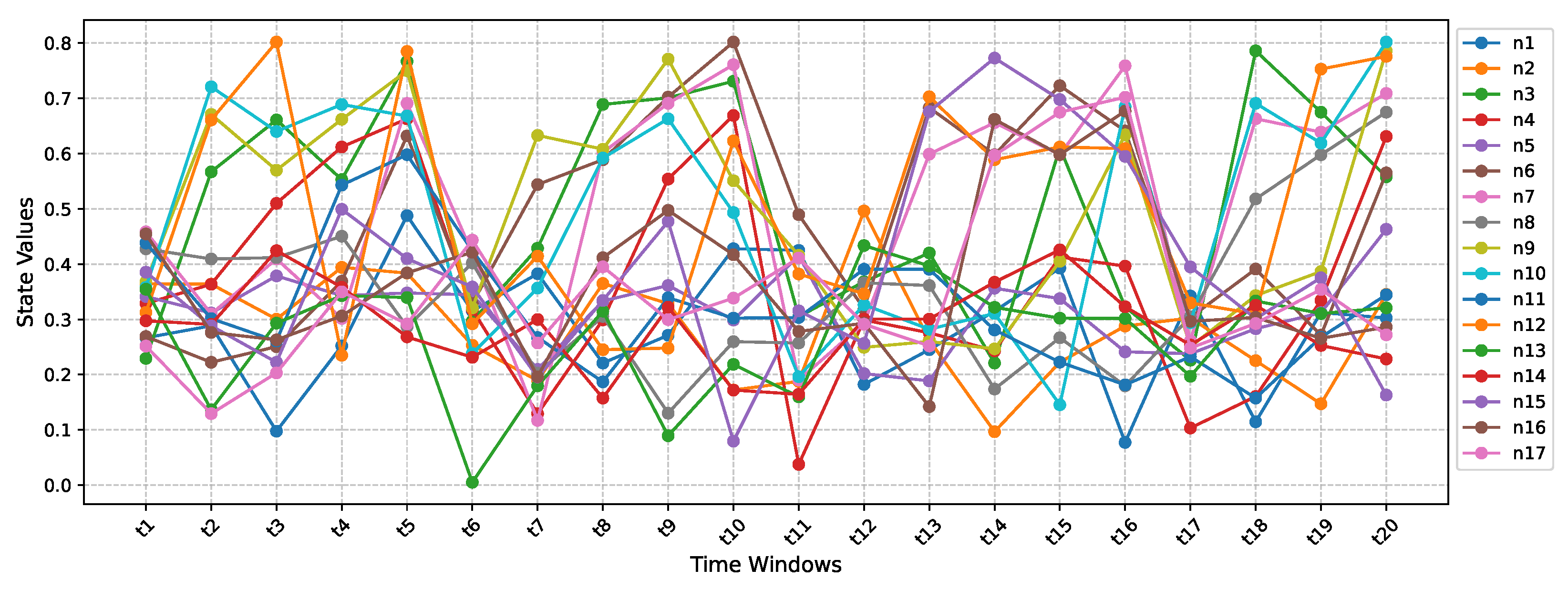
3.2. Node State Time-Series Matrix
4. Network Spatio-Temporal Situational Assessment Method Based on Anomaly Events
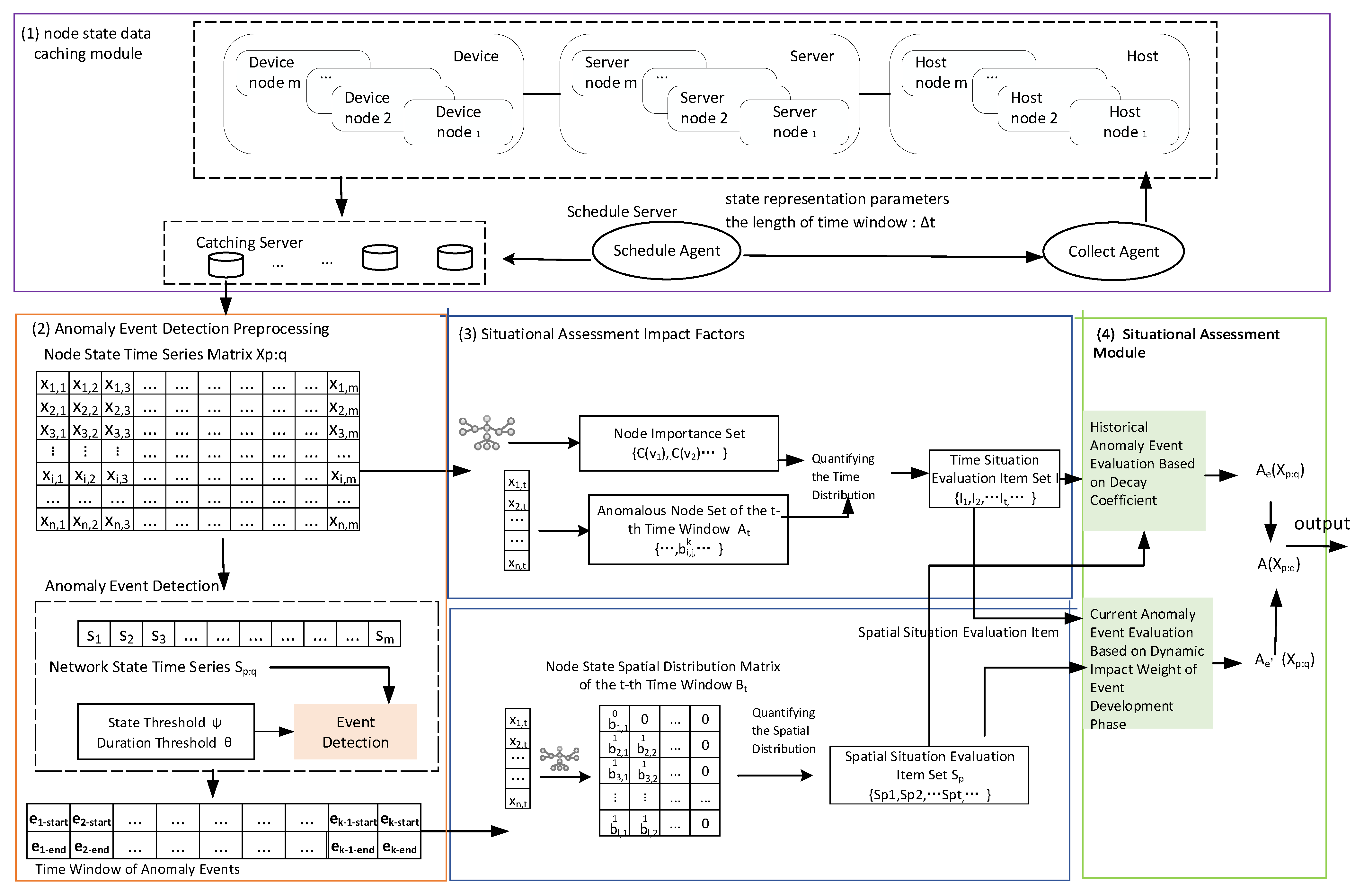
4.1. Situational Assessment Model
- (1)
- Node State Data Caching
- (2)
- Anomaly Event Detection Preprocessing
- (3)
- Situational Assessment Impact Factors
- (4)
- Situational Assessment Module
4.2. Anomaly Event Detection Preprocessing Based on State Fluctuations
- (1)
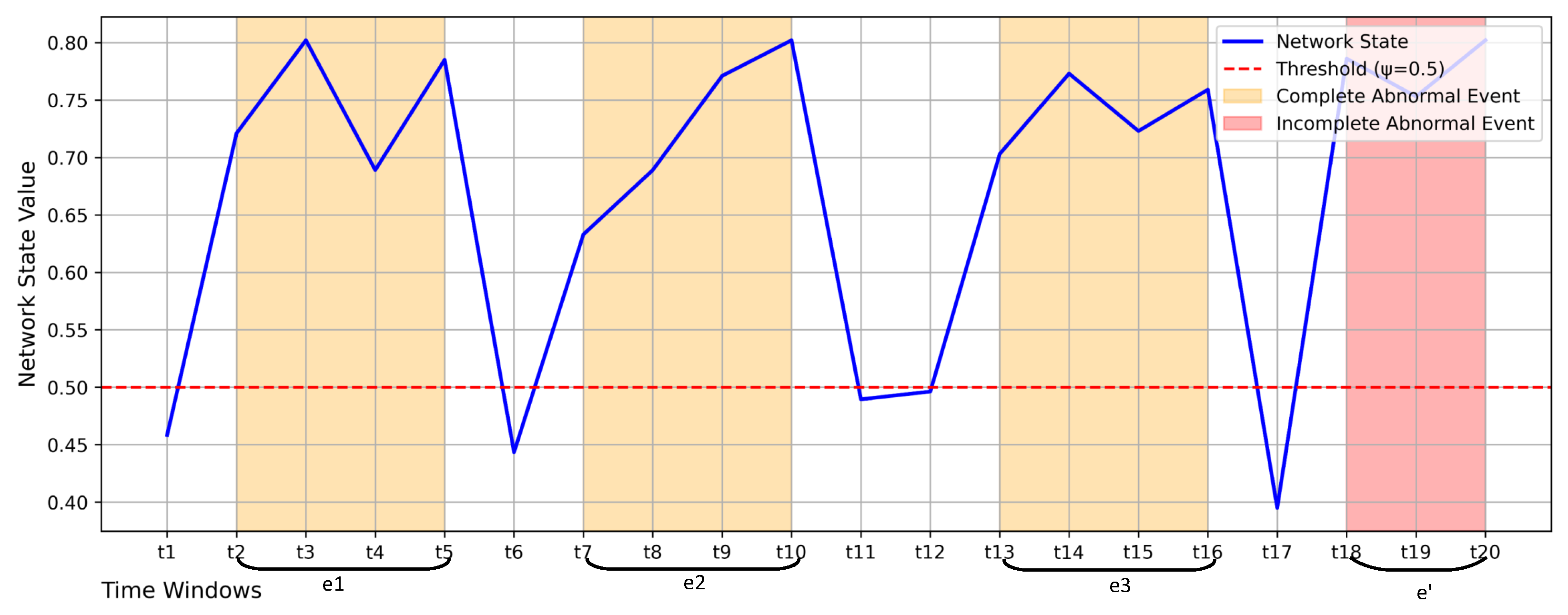
- Network State
- (2)
- Anomaly Event Determination Criteria
- (3)
- Anomaly Event Detection Preprocessing Algorithm
- Event Start: When the network state first exceeds the threshold , the start time of the event is marked.
- Event End: If the network state drops below the threshold again and the duration of the anomaly event meets the minimum threshold , this time period is marked as a historical anomaly event.
- Historical Anomaly Event Output: After traversing the network state time-series data , the algorithm outputs the start and end time windows of all detected historical anomaly events.
- Current Anomaly Event: If the network state in the last time window of the time-series data exceeds the threshold , it indicates that the anomaly event is ongoing and not yet finished. The algorithm outputs the start time window of the current anomaly event.
4.3. Spatio-Temporal Situational Impact Assessment
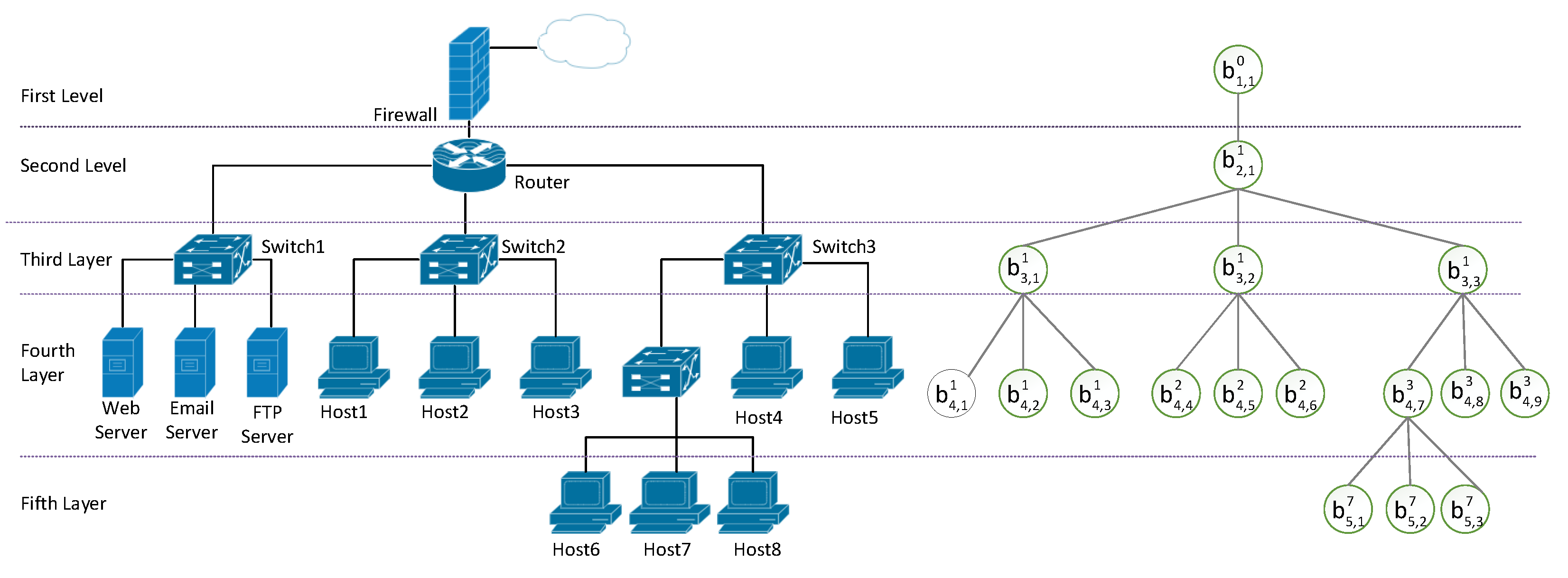
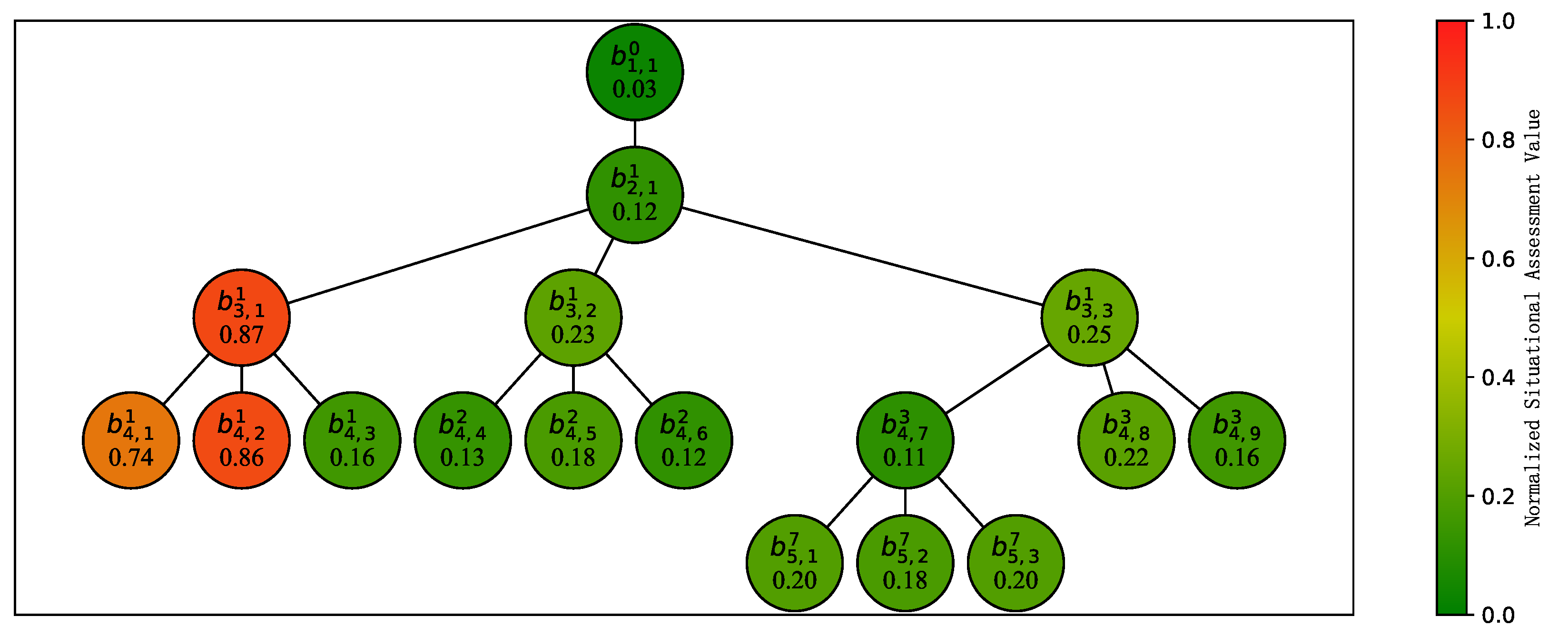
4.3.1. Node State Spatial Distribution Matrix for Time Windows
4.3.2. Abnormal Node Set for Time Windows
- For the node state spatial distribution matrix , check the state value of each node in the matrix to determine whether it exceeds the predefined threshold .
- If the state value of a node exceeds the threshold, add the node to the abnormal node set .
- Finally, the abnormal node set contains all nodes in whose state values exceed the threshold .
4.3.3. Node Importance
4.3.4. Quantifying Changes in Abnormal Node Spatial Distribution
- Domain Definition
- 2.
- Four Types of Spatial Distribution Abnormal Situations
- (1)
- Spatial Single-Point Abnormal Situation
- (2)
- Spatial Scattered-Point Abnormal Situation
- (3)
- Spatial Single-Domain Abnormal Situation
- (4)
- Spatial Multi-Domain Abnormal Situation
- 3.
- Situational Impact Assessment Value of Spatial Domains
- 4.
- Changes in the Spatial Distribution of Abnormal Nodes Across Adjacent Time Windows
- (1)
- Spatial Distribution Quantification Value for Single-Point or Scattered-Point Abnormal Situations
- (2)
- Spatial Distribution Quantification Value for Single-Domain or Multi-Domain Abnormal Situations
- (3)
- Spatial Distribution Change
4.3.5. Changes in Abnormal Node State Values Across Adjacent Time Windows
4.3.6. Situational Assessment Method
- (1)
- Situational Assessment of Historical Anomaly Event Windows
- (2)
- Situational Assessment of the Current Anomaly Event Window
5. Evaluation
5.1. Experimental Settings
5.2. Experimental Simulation and Validation
- (1)
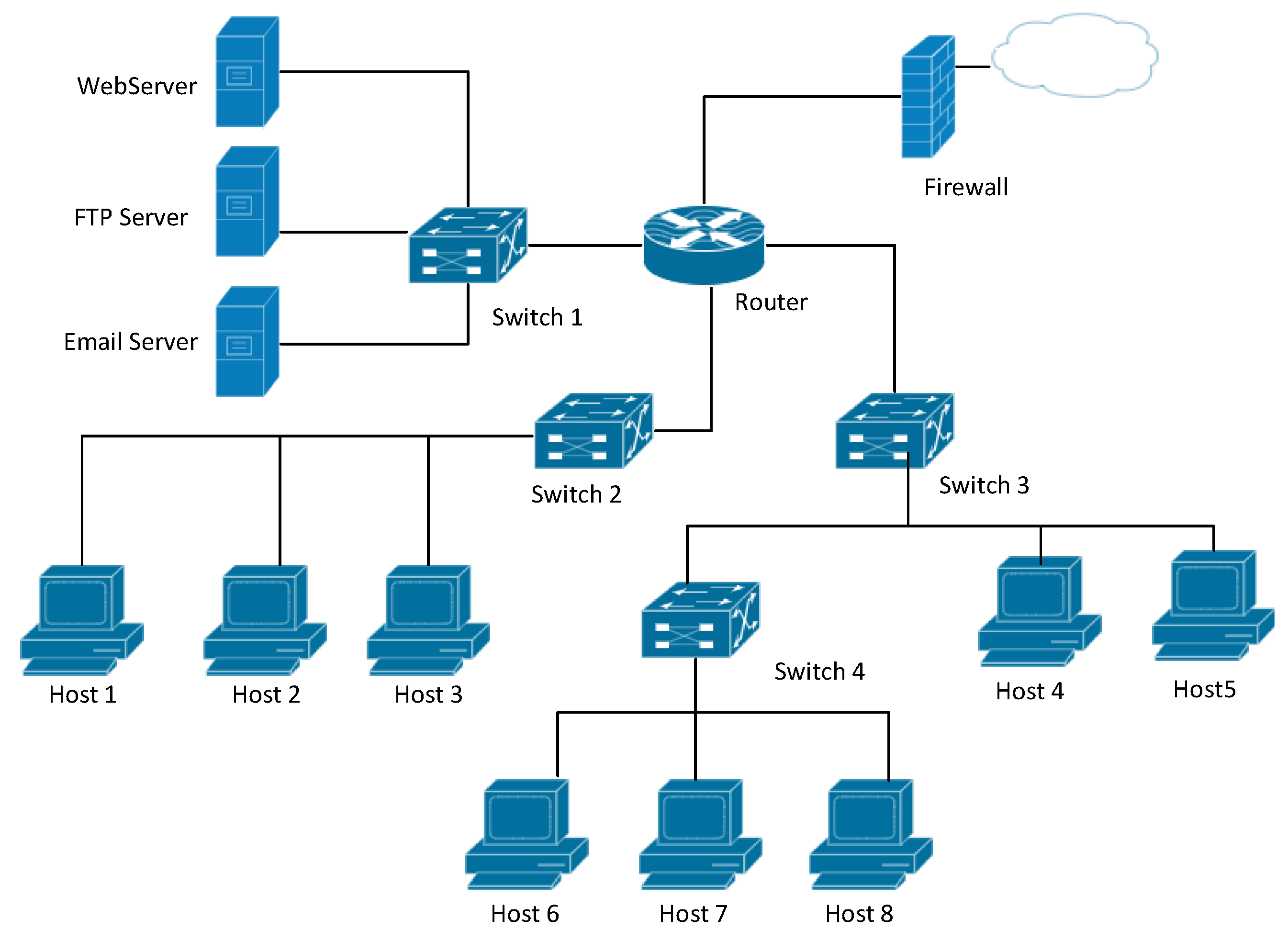
- Experimental Setup
- (2)
- Anomaly Event Detection and Preprocessing
- (3)
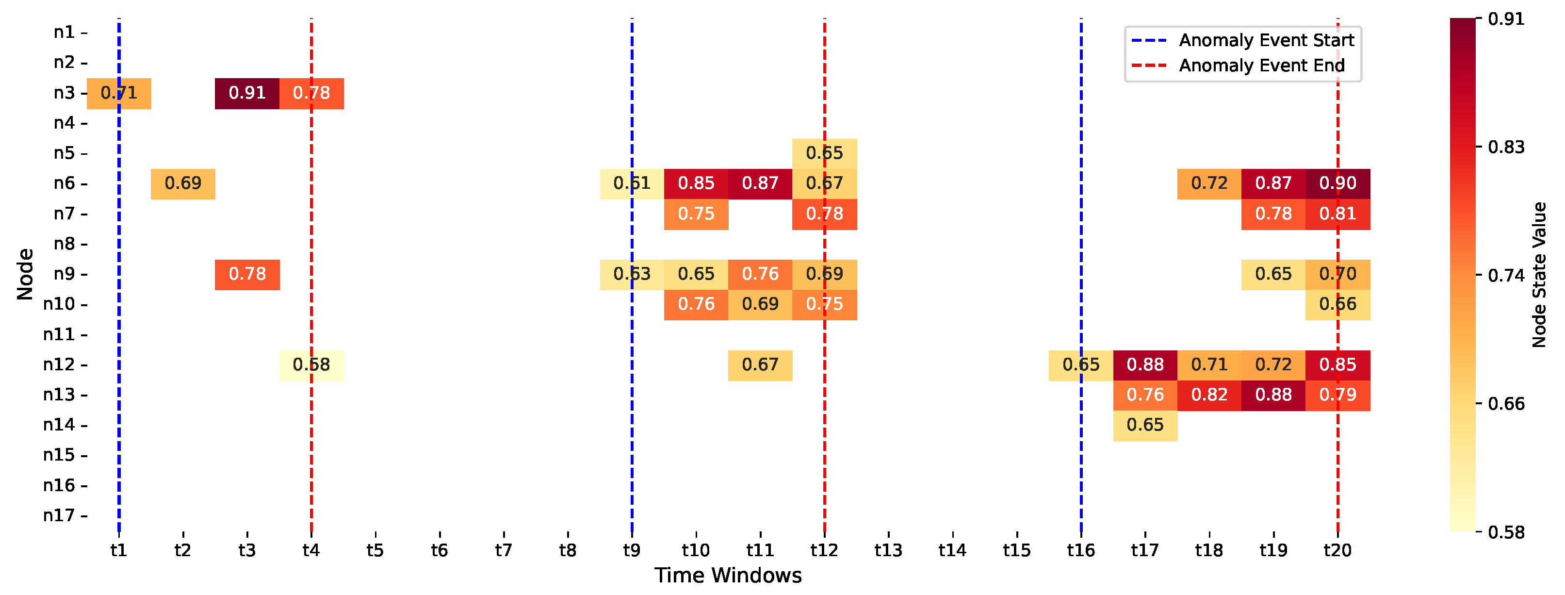
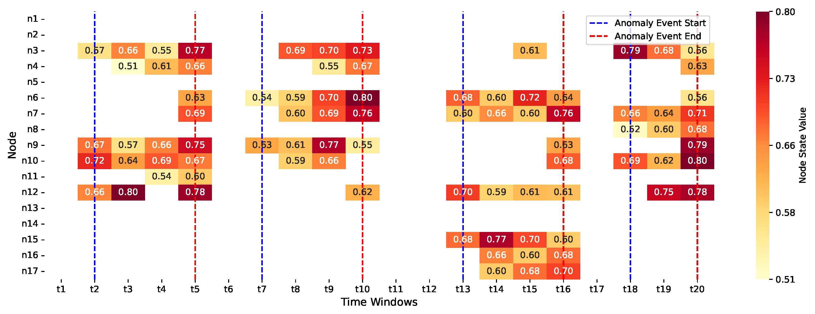
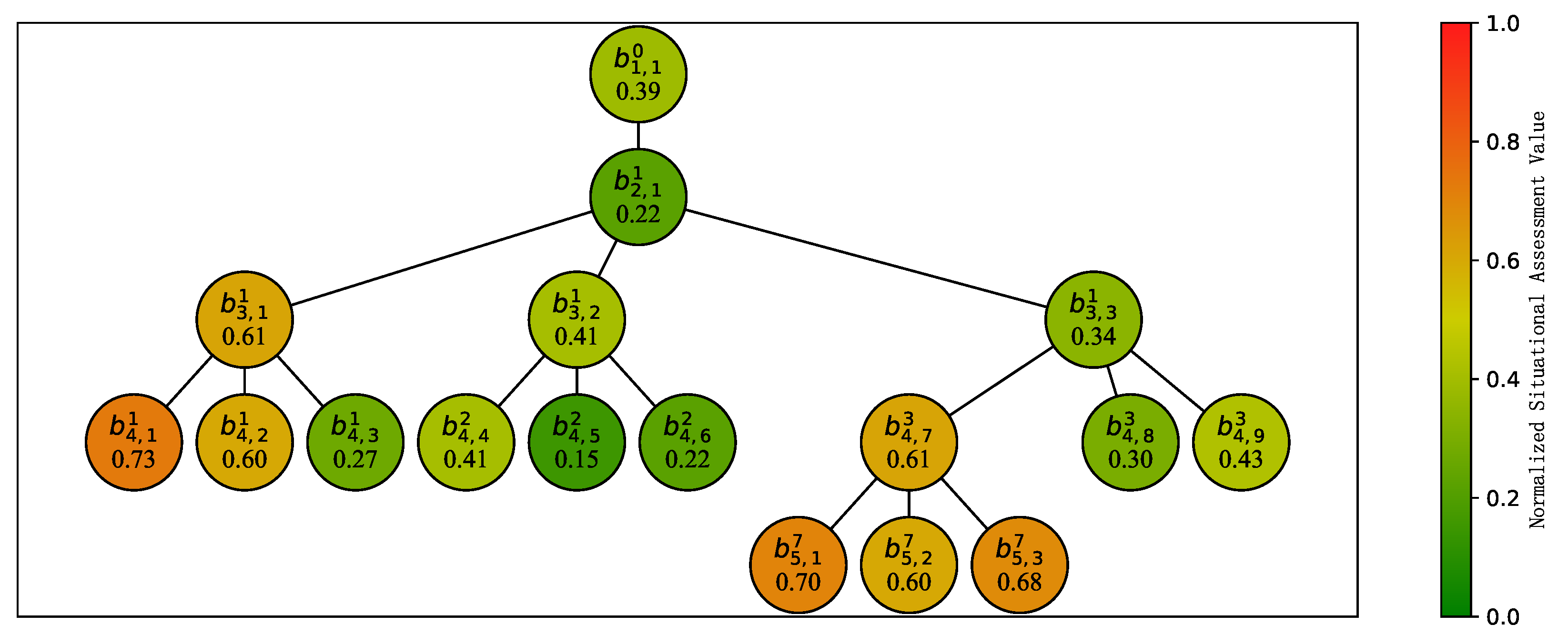
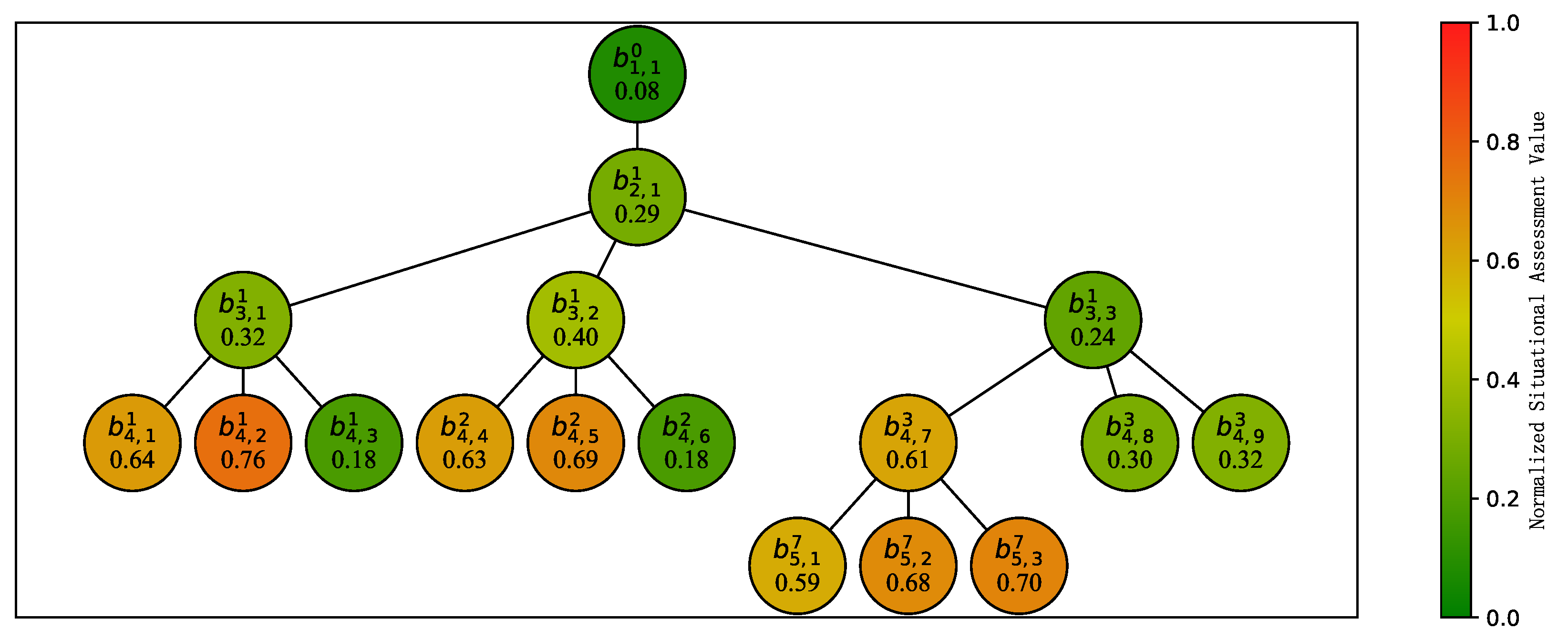
- Distribution of Abnormal Node States Within Anomaly Event Time Windows
- (4)
- Quantitative Assessment of Spatial Distribution and Node State Values
- (5)
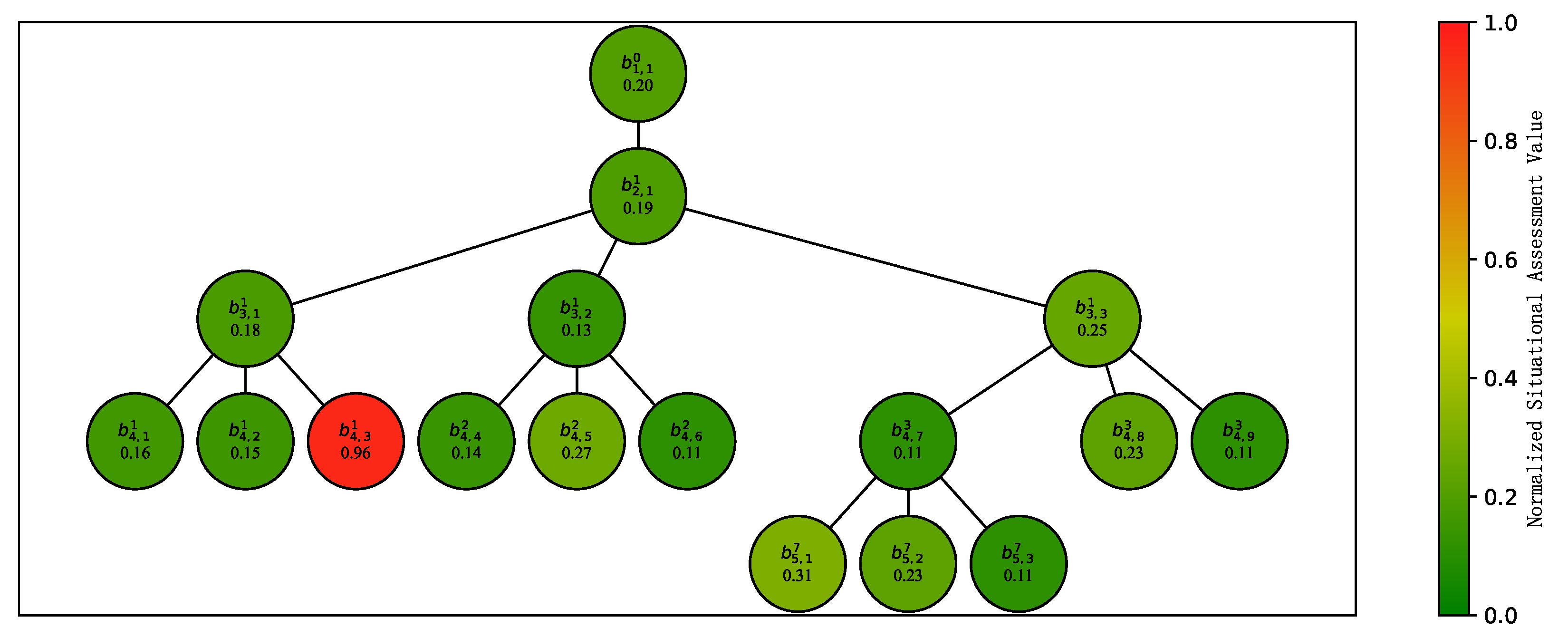
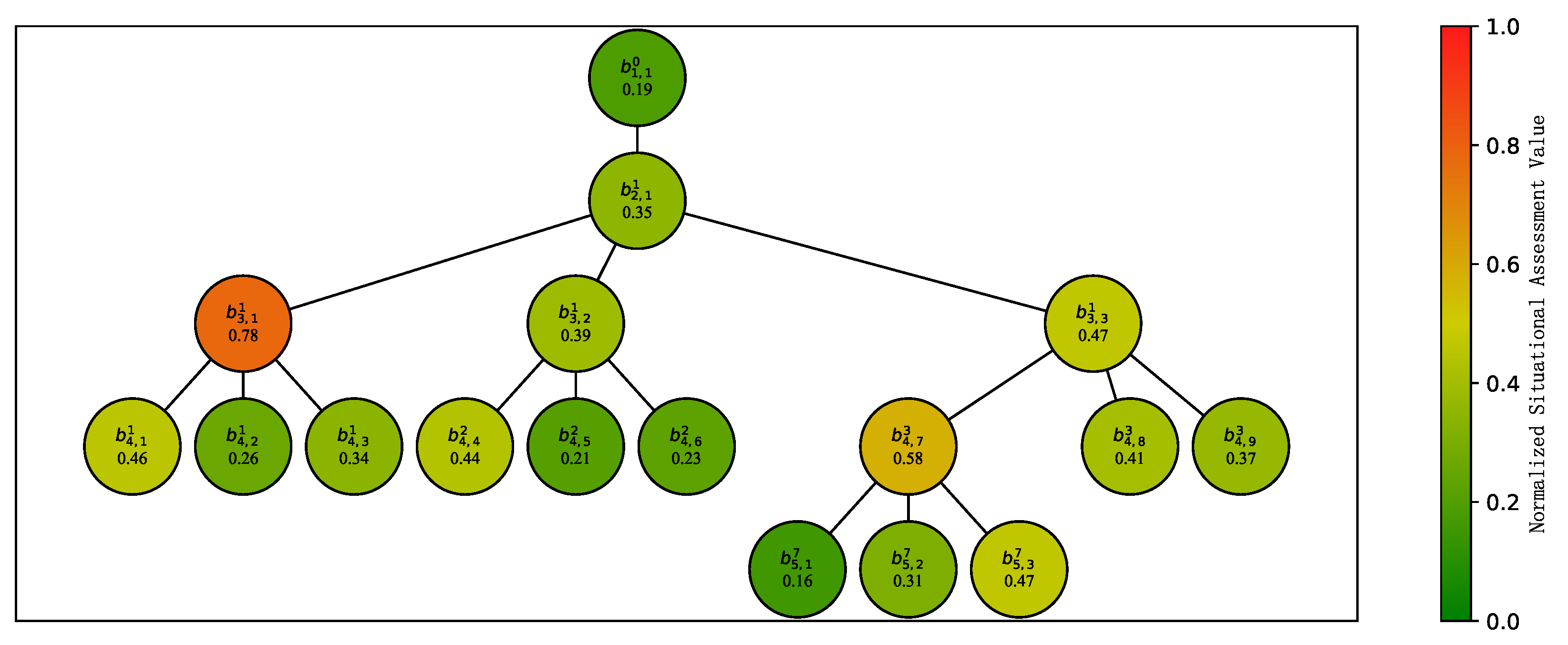
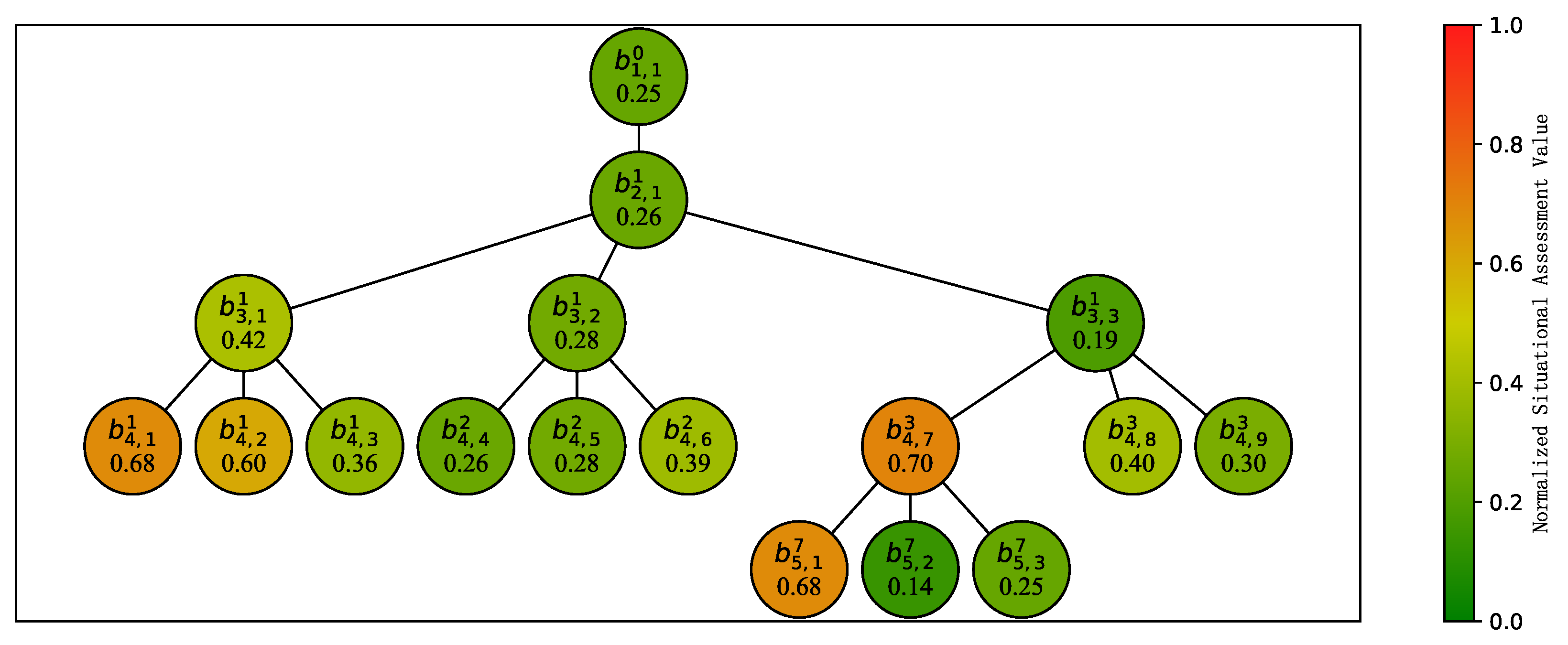
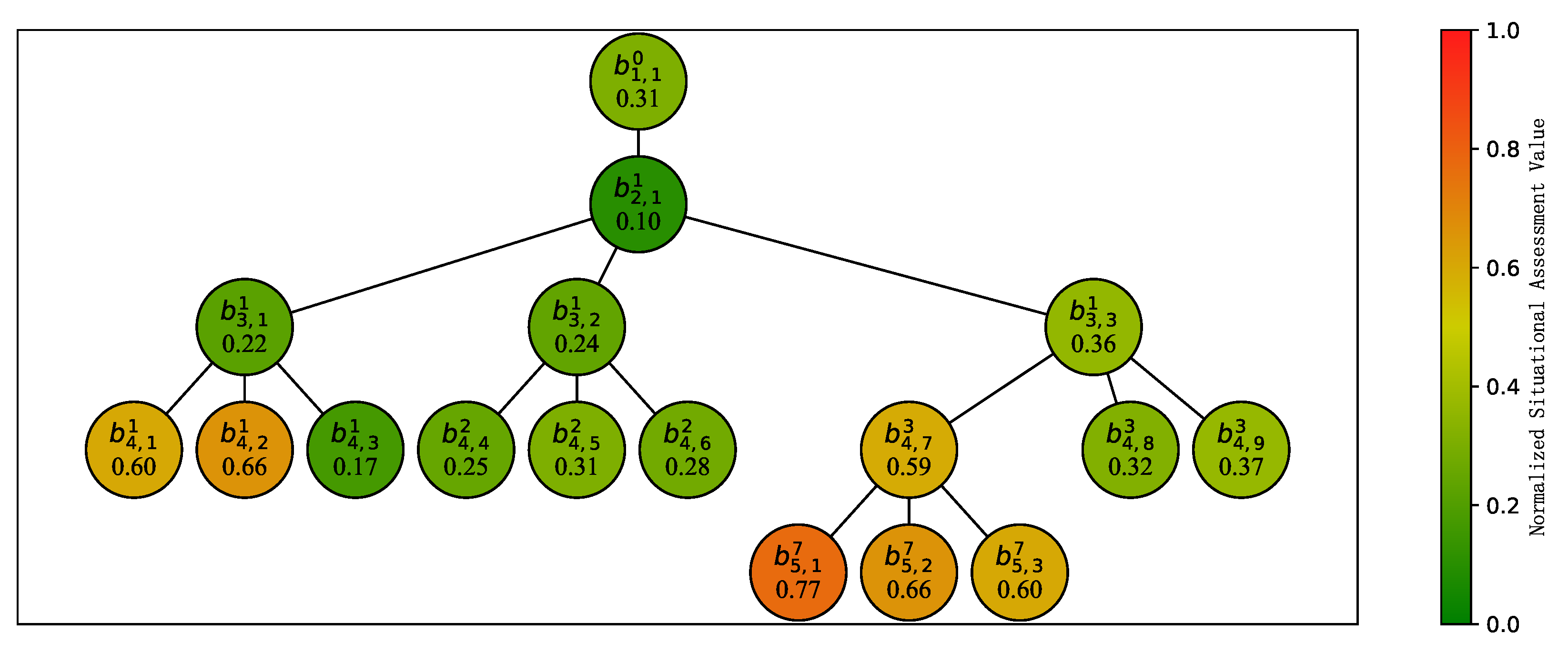
- Situational Assessment Based on Decay and Event Development Phases
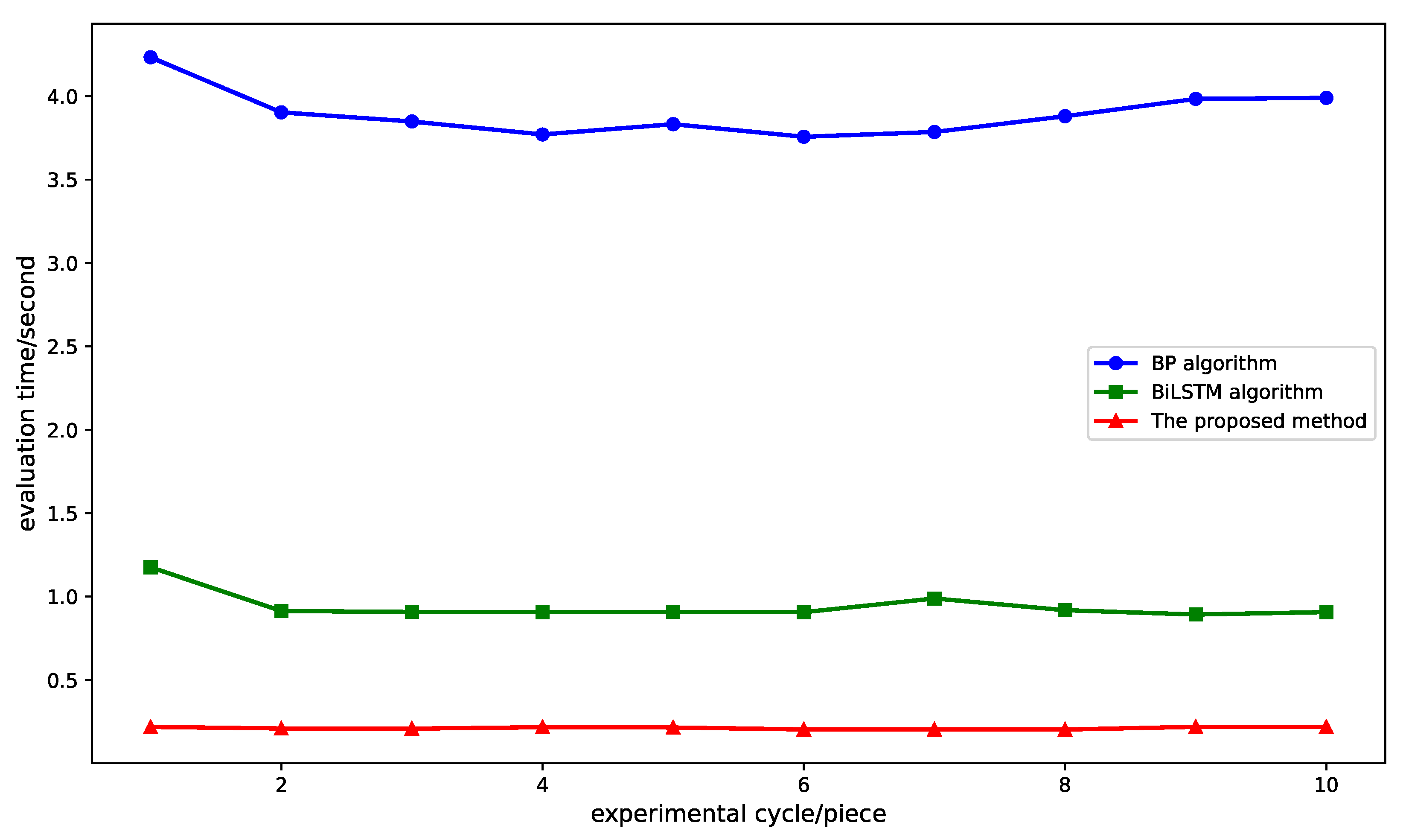
5.3. Validation of Method Effectiveness
6. Conclusions
Funding
Data Availability Statement
Conflicts of Interest
References
- Zhang, J.; Feng, H.; Liu, B.; Zhao, D. Survey of technology in network security situation awareness. Sensors 2023, 23, 2608. [Google Scholar] [CrossRef] [PubMed]
- Alavizadeh, H.; Jang-Jaccard, J.; Enoch, S.Y.; Al-Sahaf, H.; Welch, I.; Camtepe, S.A.; Kim, D.D. A survey on cyber situation-awareness systems: Framework, techniques, and insights. ACM Comput. Surv. 2022, 55, 1–37. [Google Scholar] [CrossRef]
- Barona Lopez, L.I.; Valdivieso Caraguay, A.L.; Maestre Vidal, J.; Sotelo Monge, M.A.; García Villalba, L.J. Towards incidence management in 5G based on situational awareness. Future Internet 2017, 9, 3. [Google Scholar] [CrossRef]
- Alghushairy, O.; Alsini, R.; Alhassan, Z.; Alshdadi, A.A.; Banjar, A.; Yafoz, A.; Ma, X. An efffcient support vector machine algorithm based network outlier detection system. IEEE Access 2024, 12, 24428–24441. [Google Scholar] [CrossRef]
- Bellavista, P.; Giannelli, C.; Montenero, D.D.P. A reference model and prototype implementation for SDN-based multi layer routing in fog environments. IEEE Trans. Netw. Serv. Manag. 2020, 17, 1460–1473. [Google Scholar] [CrossRef]
- Gallagher, M.; Pitropakis, N.; Chrysoulas, C.; Papadopoulos, P.; Mylonas, A.; Katsikas, S. Investigating machine learning attacks on financial time series models. Comput. Secur. 2022, 123, 102933. [Google Scholar] [CrossRef]
- Zhang, Y.; Zhang, R.; Liu, J. Network security situation assessment using deep self-encoding networks. Comput. Eng. Appl. 2020, 56, 92–98. [Google Scholar]
- Zhi, W.W.; Zhou, X.X.; Yang, L. Application of fuzzy comprehensive method and analytic hierarchy process in the evaluation of network security level protection research. Proc. J. Phys. Conf. Ser. 2021, 1820, 012187. [Google Scholar] [CrossRef]
- Zhang, S.; Fu, Q.; An, D. Network Security Situation Prediction Model Based on VMD Decomposition and DWOA Optimized BiGRU-ATTN Neural Network. IEEE Access 2023, 11, 129507–129535. [Google Scholar] [CrossRef]
- Zhao, D.; Song, H.; Zhang, H. Network Security Situation Based on Time Factor and Composite CNN Structure. Comput. Sci. 2021, 48, 349–356. [Google Scholar]
- Zhang, H.; Kang, C.; Xiao, Y. Research on network security situation awareness based on the LSTM-DT model. Sensors 2021, 21, 4788. [Google Scholar] [CrossRef] [PubMed]
- Yang, J.; Yang, Y.; Zheng, L.; Cheng, R.; Lin, S. Network security situation assessment based on attack graph techniques. J. Phys. Conf. Ser. 2022, 2310, 012071. [Google Scholar] [CrossRef]
- Chen, L.; Lü, L.; Yang, X. A Network Security Situation Assessment Method Based on Improved CRITIC and Grey Relational Analysis. Telecommun. Eng. 2022, 62, 517–525. [Google Scholar]
- Xu, Z.; Chen, J.; Zhang, Z.; Wan, J.; Yuan, P. Network Security Situation Assessment Based on Artificial Immunity and Hidden Markov Model in New Power Systems. J. East China Norm. Univ. (Nat. Sci. Ed.) 2023, 2023, 182. [Google Scholar]
- Xu, J.; Feng, B. Quantitative Assessment of Wireless Network Security Situation Based on Evidence Reasoning. Comput. Simul. 2023, 40, 449–452, 458. [Google Scholar]
- Yang, Q.; Wang, Y.; Li, S.; Yang, C.; Li, G.; Yuan, Y. A Security Evaluation Model of the Industrial Internet Based on a Selection Covariance Matrix. IEEE Access 2024, 12, 133770–133783. [Google Scholar] [CrossRef]
- Xiao, P.; Wang, K.; Huang, Z. Power Information Network Security Situation Assessment Based on IABC and Clustering Optimized RBF Neural Network. Smart Power 2022, 50, 100–106. [Google Scholar]
- Zhang, R.; Pan, Z.; Yin, Y.; Cai, Z. Network Security Situation Assessment Model Based on SAA-SSA-BPNN. Comput. Eng. Appl. 2022, 58, 117–124. [Google Scholar] [CrossRef]
- Yang, H.; Zhang, Z.; Zhang, L. Network Security Situation Assessment Based on Parallel Feature Extraction and Improved BiGRU. J. Tsinghua Univ. (Nat. Sci. Ed.) 2022, 62, 842–848. [Google Scholar]
- Ren, G.; Mo, X. Network Security Situation Assessment Based on PRFGRFECV Feature Selection and GAGLight GBM. Comput. Sci. 2023, 50, 769–774. [Google Scholar]
- Xie, B.; Li, F.; Li, H.; Wang, L.; Yang, A. Enhanced Internet of Things Security Situation Assessment Model with Feature Optimization and Improved SSA-LightGBM. Mathematics 2023, 11, 3617. [Google Scholar] [CrossRef]
- Sun, J.; Li, C.; Cao, B. Network Security Situation Prediction Based on TCN-BiLSTM. Syst. Eng. Electron. 2023, 45, 3671–3679. [Google Scholar]
- Chen, Q.; Xu, H.; Xiong, W.; Liu, W. Network Security Situation Assessment Method Based on MIDBO-SVR. Modern Electron. Technol. 2024, 1–6. [Google Scholar]
- Zhao, D.; Sun, M.; Su, M.; Wu, Y. Network Security Situation Assessment Based on Improved SKNet-SVM. J. Appl. Sci. 2024, 42, 334–349. [Google Scholar]
- Guo, S.; Liu, S.; Li, Z.; Ouyang, D.; Wang, N.; Xiang, T. Network Security Situation Awareness Method Based on Fusion Model. Comput. Eng. 2024, 50, 1–9. [Google Scholar]
- Peng, X.; Yuan, L.; Yu, Y.; Ma, Z.; Zhang, K. IoT Security Situation Assessment Based on Deep Learning. Comput. Appl. Softw. 2024, 1–9. [Google Scholar]
- Ullah, W.; Hussain, T.; Khan, Z.A.; Haroon, U.; Baik, S.W. Intelligent dual stream CNN and echo state network for anomaly detection. Knowl.-Based Syst. 2022, 253, 109456. [Google Scholar] [CrossRef]
- Sun, Y.; Ma, P.; Dai, J.; Li, D. A cloud Bayesian network approach to situation assessment of scouting underwater targets with fixed-wing patrol aircraft. CAAI Trans. Intell. Technol. 2023, 8, 532–545. [Google Scholar] [CrossRef]
- Fan, Z.; Xiao, Y.; Nayak, A.; Tan, C. An improved network security situation assessment approach in software defined networks. Peer-to-Peer Netw. Appl. 2019, 12, 295–309. [Google Scholar] [CrossRef]


| Approach | Year | Author(s) | Characteristics |
|---|---|---|---|
| Mathematical Mode | 2022 | Jinwei Yang et al. [12] | Assessment method based on attack graph |
| Mathematical Mode | 2022 | Chen Long et al. [13] | Using improved CRITIC and gray correlation analysis |
| Mathematical Mode | 2023 | Xu Zhi et al. [14] | Using hidden Markov and artificial immunization |
| Mathematical Mode | 2023 | Xu Jian et al. [15] | Assessment method based on evidential reasoning |
| Mathematical Mode | 2024 | QingQing Yang et al. [16] | Using a selection covariance matrix process |
| Machine Learning | 2022 | Xiao Peng et al. [17] | Assessment method based on IABC and clustering |
| Machine Learning | 2022 | Zhang Ran et al. [18] | Assessment model based on SAA-SSA-BPNN |
| Machine Learning | 2022 | Yang Hongyu et al. [19] | Assessment method based on parallel feature extraction network and attention mechanism improved BiGRU |
| Machine Learning | 2023 | Ren Gaoke et al. [20] | Using GA-LightGBM based on PRF-RFECV feature optimization |
| Machine Learning | 2023 | Baoshan Xie et al. [21] | Using feature optimization and improved SSA-LightGBM |
| Machine Learning | 2023 | Sun Junfeng et al. [22] | Using TCP-BiLSTM |
| Machine Learning | 2024 | Chen Qiuqiong et al. [23] | Assessment method based on MIDBO-SVR |
| Machine Learning | 2024 | Zhao Dongmei et al. [24] | Assessment model based on improved selective kernel convolutional neural network and support vector machine |
| Machine Learning | 2024 | Guo Shangwei et al. [25] | Assessment method based on fusion model |
| Machine Learning | 2024 | Peng Xingwei et al. [26] | Assessment method based on deep learning |
| Node | n1 | n2 | n3 | n4 | n5 | n6 | n7 | n8 | n9 |
| Importance | 0.0539 | 0.1407 | 0.0962 | 0.0962 | 0.1211 | 0.0368 | 0.0368 | 0.0368 | 0.0368 |
| Node | n10 | n11 | n12 | n13 | n14 | n15 | n16 | n17 | |
| Importance | 0.0368 | 0.0368 | 0.0828 | 0.0464 | 0.0464 | 0.0317 | 0.0317 | 0.0317 |
| Anomaly Event | Time Window | Anomalous Nodes | Spatial Distribution Type | Anomalous Node State Value per Time Window | Spatial Distribution Value per Time Window |
|---|---|---|---|---|---|
| t1 | n3 | A1 | 0.068302 | 0.0962 | |
| t2 | n6 | A1 | 0.025392 | 0.0368 | |
| t3 | n3, n7 | A2 | 0.116246 | 0.133 | |
| t4 | n6, n7, n8 | A2 | 0.076544 | 0.1104 | |
| t9 | n6, n9 | A2 | 0.045632 | 0.0736 | |
| t10 | n6, n7, n9, n10 | A2 | 0.110768 | 0.08704 | |
| t11 | n6, n9, n10, n12 | A2 | 0.140852 | 0.1932 | |
| t12 | n5, n6, n7, n9, n10 | A2 | 0.185067 | 0.2683 | |
| t16 | n12 | A1 | 0.05382 | 0.0828 | |
| t17 | n12, n13, n14 | A2 | 0.138288 | 0.1756 | |
| t18 | n12, n13, n6 | A2 | 0.123332 | 0.166 | |
| t19 | n12, n13, n6, n7, n9 | A2 | 0.185088 | 0.2396 | |
| t20 | n12, n13, n6, n7, n9, n10 | A2 | 0.220012 | 0.2764 |
| Anomaly Event | Time Window | Anomalous Nodes | Spatial Distribution Type | Anomalous Node State Value per Time Window | Quantitative Value of Spatial Distribution per Time Window |
|---|---|---|---|---|---|
| t2 | n3, n9, n10, n12 | A2 | 0.1605018 | 0.2526 | |
| t3 | n3, (n4, n9, n10), n12 | A3 | 0.2235838 | 2.5047 | |
| t4 | n3, (n4, n9, n10, n11) | A3 | 0.1817722 | 3.8940 | |
| t5 | (n3, n6, n7), (n4, n9, n10, n11), n12 | A4 | 0.3254392 | 6.1702 | |
| t7 | n6, n9 | A2 | 0.0433136 | 0.0736 | |
| t8 | (n3, n6, n7), n9, n10 | A3 | 0.1542706 | 2.3993 | |
| t9 | (n3, n6, n7), (n4, n9, n10) | A4 | 0.2247756 | 4.6515 | |
| t10 | (n3, n6, n7), (n4, n9), n12 | A4 | 0.2640596 | 3.8342 | |
| t13 | n6, n7, (n12, n15) | A3 | 0.1268152 | 1.4900 | |
| t14 | n6, n7, (n12, n15, n16, n17) | A3 | 0.1593308 | 3.8571 | |
| t15 | (n3, n6, n7), (n12, n15, n16, n17) | A4 | 0.2205453 | 6.1092 | |
| t16 | (n3, n6, n7), (n4, n9, n10), (n12, n15, n16, n17) | A4 | 0.2130602 | 8.4350 | |
| t18 | (n3, n7, n8), n10 | A3 | 0.1445028 | 2.3625 | |
| t19 | (n3, n7, n8), n10, n12 | A3 | 0.1955842 | 2.4453 | |
| t20 | (n3, n6, n7, n8), (n4, n9, n10), n12 | A4 | 0.3087962 | 6.2064 |
| Anomaly Event | From Time Window | To Time Window | |||||
|---|---|---|---|---|---|---|---|
| t1 | t2 | −0.04291 | −0.0594 | −2.87 | −2.40 | −3.33 | |
| t2 | t3 | 0.090854 | 0.0962 | 1.42 | 1.38 | 1.47 | |
| t3 | tt4 | −0.039702 | −0.0226 | −1.29 | −1.64 | −9.36 | |
| t9 | t10 | 0.065136 | 0.7968 | 7.20 | 1.09 | 1.33 | |
| t10 | t11 | 0.030084 | −0.6772 | −1.47 | 1.37 | −3.07 | |
| t11 | t12 | 0.044215 | 0.0751 | 7.36 | 5.46 | 9.27 | |
| t16 | t17 | 0.084468 | 0.0928 | 0.6549216 | 0.6241388 | 0.6857044 | |
| t17 | t18 | −0.014956 | −0.0096 | −0.0333751 | −0.0406546 | −0.0260955 | |
| t18 | t19 | 0.061756 | 0.0736 | 0.1839679 | 0.1678702 | 0.2000655 | |
| t19 | t20 | 0.034924 | 0.0368 | 0.1607223 | 0.1565185 | 0.1649262 |
| Anomaly Event | From Time Window | To Time Window | |||||
|---|---|---|---|---|---|---|---|
| t2 | t3 | 0.063082 | 2.2521 | 1.76 | 9.61 | 3.43 | |
| t3 | t4 | −0.0418116 | 1.3893 | 2.79 | −1.73 | 5.75 | |
| t4 | t5 | 0.143667 | 2.2762 | 1.36 | 1.62 | 2.56 | |
| t7 | t8 | 0.110957 | 2.3257 | 2.75 | 2.51 | 5.26 | |
| t8 | t9 | 0.07050504 | 2.2521 | 7.14 | 4.33 | 1.38 | |
| tt9 | t10 | 0.03928396 | −0.8173 | −6.50 | 6.56 | −1.37 | |
| t13 | t14 | 0.0325156 | 2.3671 | 0.0010941 | 2.97 | 0.0021585 | |
| t14 | t15 | 0.0612145 | 2.2521 | 0.0028671 | 1.52 | 0.0055825 | |
| t15 | t16 | −0.0074851 | 2.3257 | 0.0078102 | −5.04 | 0.0156707 | |
| t18 | t19 | 0.0510814 | 0.0828 | 0.1819637 | 0.1388536 | 0.2250737 | |
| t19 | t20 | 0.113212 | 3.7610 | 14.313489 | 0.8365298 | 27.790447 |
Disclaimer/Publisher’s Note: The statements, opinions and data contained in all publications are solely those of the individual author(s) and contributor(s) and not of MDPI and/or the editor(s). MDPI and/or the editor(s) disclaim responsibility for any injury to people or property resulting from any ideas, methods, instructions or products referred to in the content. |
© 2025 by the author. Licensee MDPI, Basel, Switzerland. This article is an open access article distributed under the terms and conditions of the Creative Commons Attribution (CC BY) license (https://creativecommons.org/licenses/by/4.0/).
Share and Cite
Xiao, P. A Network Security Situational Assessment Method Considering Spatio-Temporal Correlations. Symmetry 2025, 17, 385. https://doi.org/10.3390/sym17030385
Xiao P. A Network Security Situational Assessment Method Considering Spatio-Temporal Correlations. Symmetry. 2025; 17(3):385. https://doi.org/10.3390/sym17030385
Chicago/Turabian StyleXiao, Ping. 2025. "A Network Security Situational Assessment Method Considering Spatio-Temporal Correlations" Symmetry 17, no. 3: 385. https://doi.org/10.3390/sym17030385
APA StyleXiao, P. (2025). A Network Security Situational Assessment Method Considering Spatio-Temporal Correlations. Symmetry, 17(3), 385. https://doi.org/10.3390/sym17030385