Estimation and Bayesian Prediction for the Generalized Exponential Distribution Under Type-II Censoring

Abstract

This research focuses on the prediction and estimation problems for the generalized exponential distribution under Type-II censoring. Firstly, maximum likelihood estimations for the parameters of the generalized exponential distribution are computed using the EM algorithm. Additionally, confidence intervals derived from the Fisher information matrix are developed and analyzed alongside two bootstrap confidence intervals for comparison. Compared to classical maximum likelihood estimation, Bayesian inference proves to be highly effective in handling censored data. This study explores Bayesian inference for estimating the unknown parameters, considering both symmetrical and asymmetrical loss functions. Utilizing Gibbs sampling to produce Markov Chain Monte Carlo samples, we employ an importance sampling approach to obtain Bayesian estimates and compute the corresponding highest posterior density (HPD) intervals. Furthermore, for one-sample prediction and, separately, for the two-sample case, we provide the corresponding posterior distributions, along with methods for computing point predictions and predictive intervals. Through Monte Carlo simulations, we evaluate the performance of Bayesian estimation in contrast to maximum likelihood estimation. Finally, we conduct an analysis of a real dataset derived from deep groove ball bearings, calculating Bayesian point predictions and predictive intervals for future samples.

1. Introduction

In 1999, Reference [1] first formally introduced the generalized exponential distribution. It can also be regarded as a particular member of the three-parameter Exponentiated Weibull (EW) distribution, introduced by Reference [2]. Furthermore, its origins can be traced back to the early work of Gompertz and Verhulst, who introduced cumulative distribution functions for modeling human mortality and population growth. Interested readers can refer to References [3,4] for more details.

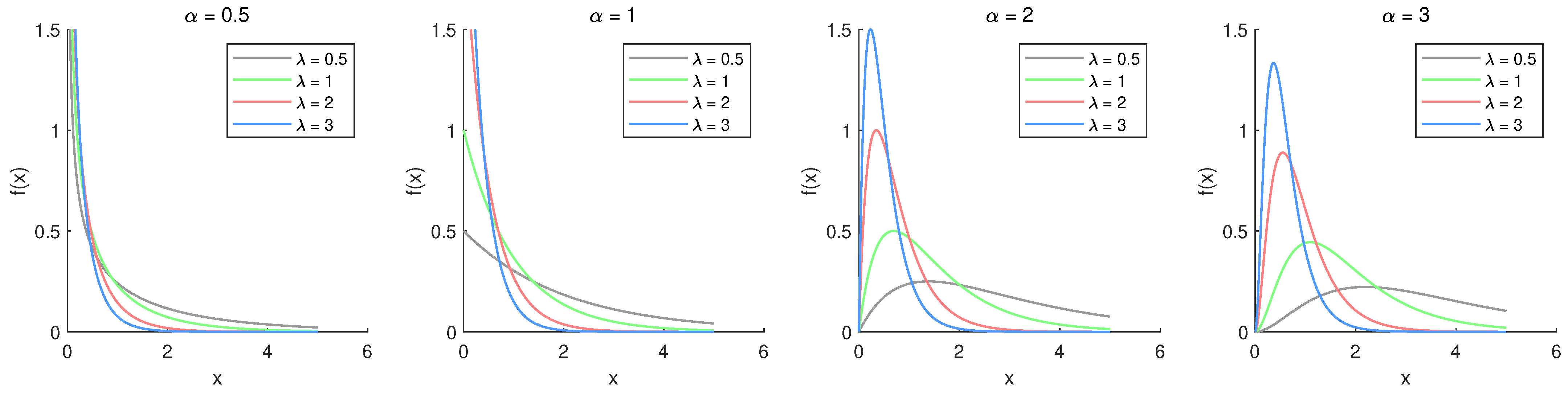
The probability density function (PDF) and cumulative distribution function (CDF) of generalized exponential distribution can be expressed as:

$$f\left(x\right)=\alpha \lambda e^{-\lambda x}{\left(1-e^{-\lambda x}\right)}^{\alpha -1},x>0,\alpha >0,\lambda >0,$$

(1)

$$F\left(x\right)={\left(1-e^{-\lambda x}\right)}^{\alpha },$$

(2)

The hazard rate and reliability functions can be expressed as:

$$h\left(x\right)={\displaystyle \frac{\alpha \lambda e^{-\lambda x}{(1-e^{-\lambda x})}^{\alpha -1}}{1-{(1-e^{-\lambda x})}^{\alpha }}},$$

(3)

$$R\left(x\right)=1-{(1-e^{-\lambda x})}^{\alpha }.$$

(4)

Figure 1 illustrates the PDF plots for the chosen parameter values. Based on Figure 1, the density function demonstrates different behaviors depending on $\alpha$. For $\alpha \le 1$, it is monotonically decreasing, whereas for $\alpha >1$, it becomes unimodal and right-skewed, similar to Weibull or Gamma distributions. The hazard rate plots with different parameter values are shown in Figure 2. It shows that the hazard function decreases when $\alpha <1$, remains constant when $\alpha =1$, and increases when $\alpha >1$. Notably, the hazard function eventually converges to the value of $\lambda$.

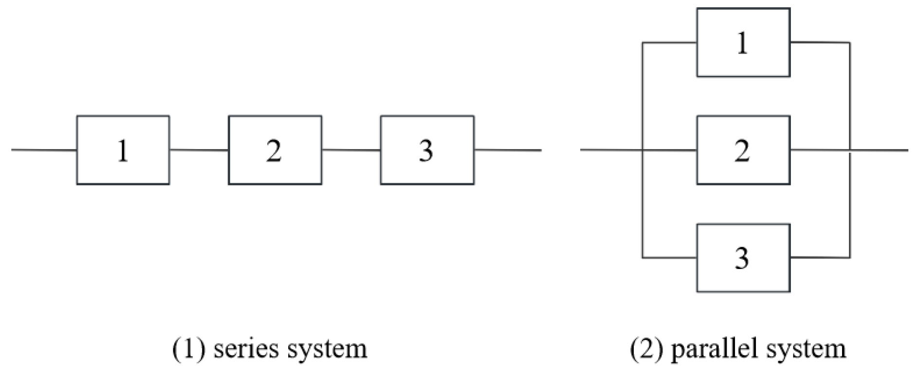
There are some interesting physical interpretations for the generalized exponential distribution. It defines the distribution of the maximum among $\alpha$ random variables that are independently and exponentially distributed when $\alpha$ is a positive integer greater than 1. This distribution applies to situations such as the overall lifetime of parallel systems of electronic components, each with an exponential lifetime distribution. In contrast, for a series system, the overall lifetime corresponds to the minimum of the exponentially distributed lifetimes, which follows an exponential distribution with rate parameter $\alpha \lambda$. Figure 3 presents a schematic representation of both series and parallel systems.

The generalized exponential distribution has gained significant scholarly interest due to its practical importance, particularly in situations involving censored data. This attention has led to a wealth of research focusing on its statistical properties. Reference [1] conducted a comprehensive study of its properties, addressing maximum likelihood estimation (MLE) along with its asymptotic behavior and issues related to hypothesis testing.

Reference [5] compared the generalized exponential distribution with the Weibull and Gamma distributions, demonstrating its advantages in modeling skewed life data. Further, Reference [6] investigated various parameter estimation methods and evaluated their performance.

Reference [7] studied estimation issues for the generalized exponential distribution under hybrid censoring, utilizing the EM algorithm to compute MLEs and importance sampling to derive Bayesian estimates. The Bayesian estimation for the parameter using doubly censored samples was derived by Reference [8]. Reference [9] applied both classical and Bayesian approaches for the estimation of parameters as well as the reliability and hazard functions based on adaptive Type-II progressive censored data. For more detailed results and examples related to the generalized exponential distribution, please refer to References [10,11,12,13].

However, research on Bayesian prediction problems remains relatively scarce for generalized exponential distribution. Prediction is an important aspect in life-testing experiments, where data from an existing sample is used to make inferences about future observations. Several studies have explored prediction problems in various contexts. For instance, Reference [14] provided a comprehensive and detailed review of Bayesian prediction techniques and their diverse applications. Additionally, Reference [15] studied one-sample and two-sample Bayesian prediction problems for the inverse Weibull distribution under Type-II censoring. Similarly, Reference [16] investigated the Poisson-Exponential distribution by employing both classical and Bayesian approaches, providing point predictions and credible predictive intervals.

This paper focuses on both one-sample and two-sample prediction problems. In the one-sample prediction case, let $X_1<\cdots <X_r$ represent the observed informative sample and $X_{r+1}<\cdots <X_n$ denote the future sample. The aim is to predict and make inferences about the future order statistics $X_k$ for $r<k\le n$. In the two-sample case, the observed sample of size r is denoted by $X_1<\cdots <X_r$, and the future ordered sample of size m is represented by $Y_1<\cdots <Y_m$. These two samples are based on the same distribution and assumed to be independent, enabling predictions and inferences for the order statistics $Y_1<\cdots <Y_m$.

The primary objectives of this study are twofold. Firstly, we aim to obtain the MLEs and Bayesian estimates under the Type-II censoring scheme and to compare their performance. Secondly, we seek to derive the Bayesian posterior predictive density for future order statistics and, based on this posterior predictive density, compute both point predictions and predictive intervals.

This paper proceeds as follows: In Section 2, the EM algorithm is employed to approximate the MLE of the model. For interval estimation, the Fisher information matrix is used to construct asymptotic confidence intervals (ACIs). Additionally, two bootstrap-based interval estimation methods are explored as comparative alternatives to evaluate their performance. Section 3 presents Bayesian parameter estimation under three different loss functions, utilizing Gibbs sampling and importance sampling techniques. HPD credible intervals are further obtained from the Gibbs sampling results. Section 4 focuses on Bayesian point predictions and the computation of predictive intervals for future order statistics. In Section 5, simulation studies are conducted to evaluate the performance of the proposed methodologies, followed by an analysis of a real-world dataset related to deep groove ball bearings, which is discussed in Section 6. Finally, we present conclusions in Section 7.

2. Maximum Likelihood Estimation

Let $x_1<x_2<\cdots <x_r$ denote a sample containing r observations obtained from the generalized exponential distribution under a Type-II censoring scheme characterized by $R=(n,r)$. The likelihood function associated with this sample is given by:

$$L(\alpha ,\lambda )={\displaystyle \frac{n!}{(n-r)!}}\prod _{i=1}^r\left(\alpha \lambda e^{-\lambda x_i}{\left(1-e^{-\lambda x_i}\right)}^{\alpha -1}\right)·{\left(1-{\left(1-e^{-\lambda x_r}\right)}^{\alpha }\right)}^{n-r}.$$

(5)

Neglecting the constant term, the log-likelihood function is:

$$l(\alpha ,\lambda )=rln\alpha \lambda +(\alpha -1)\sum _{i=1}^{r}ln\left(1-e^{-\lambda x_i}\right)-\lambda \sum _{i=1}^r{x}_i+(n-r)ln\left(1-{\left(1-e^{-\lambda x_r}\right)}^{\alpha }\right).$$

(6)

To compute the MLEs, we differentiate (6) with respect to $\alpha$ and $\lambda$ and set the derivatives to zero. The partial derivatives are:

$${\displaystyle \frac{\partial l(\alpha ,\lambda )}{\partial \alpha }}={\displaystyle \frac{r}{\alpha }}+\sum _{i=1}^{r}ln\left(1-e^{-\lambda x_i}\right)-(n-r){\displaystyle \frac{{\left(1-e^{-\lambda x_r}\right)}^{\alpha }ln\left(1-e^{-\lambda x_r}\right)}{1-{\left(1-e^{-\lambda x_r}\right)}^{\alpha }}}=0,$$

$${\displaystyle \frac{\partial l(\alpha ,\lambda )}{\partial \lambda }}={\displaystyle \frac{r}{\lambda }}+\sum _{i=1}^r{\displaystyle \frac{(\alpha -1)x_i}{e^{\lambda x_i}-1}}-\sum _{i=1}^r{x}_i-(n-r){\displaystyle \frac{\alpha {\left(1-e^{-\lambda x_r}\right)}^{\alpha -1}{e}^{-\lambda x_r}{x}_r}{1-{\left(1-e^{-\lambda x_r}\right)}^{\alpha }}}=0.$$

However, solving these equations analytically is not feasible. Therefore, numerical methods, such as the EM algorithm, are recommended. Initially introduced in Reference [17], the EM algorithm is a suitable approach for this scenario.

Under Type-II censoring framework, the observed data, represented as $X=(x_1,x_2,\cdots ,x_r)$, corresponds to the first r observations. The remaining $n-r$ data points, which are censored and unobserved, are denoted as $Z=(z_1,z_2,\cdots ,z_{n-r})$. Together, these two components form the complete sample W, where $W=(X,Z)$.

When constants are excluded, the log-likelihood function for W, represented as $L_c(\alpha ,\lambda ;W)$, can be expressed as:

$$\begin{array}{cc}\hfill L_c(\alpha ,\lambda ;W)=& nln\left(\alpha \lambda \right)-\lambda \sum _{i=1}^r{x}_i-\lambda \sum _{i=1}^{n-r}{z}_i\hfill \\ \hfill & +(\alpha -1)\sum _{i=1}^{r}ln\left(1-e^{-\lambda x_i}\right)+(\alpha -1)\sum _{i=1}^{n-r}ln\left(1-e^{-\lambda z_i}\right).\hfill \end{array}$$

(7)

The EM algorithm iteratively computes the MLEs by alternating between the E-step and M-step. In the E-step, the expectation of the log-likelihood function is calculated given the observed data X and the current parameter estimates. These estimates are updated in the M-step by maximizing the expected complete log-likelihood function. Therefore, we first derive the expression for the pseudo-log-likelihood function as follows:

$$\begin{array}{cc}\hfill L_s(\alpha ,\lambda )=& nln\alpha \lambda -\lambda \sum _{i=1}^r{x}_i+\sum _{i=1}^r(\alpha -1)ln(1-e^{-\lambda x_i})\hfill \\ \hfill & -\sum _{i=1}^{n-r}\lambda E\left(z_i\right|z_i>x_r)+\sum _{i=1}^{n-r}(\alpha -1)E(ln(1-e^{-\lambda z_i})|z_i>x_r),\hfill \end{array}$$

(8)

where

$$\begin{array}{cc}\hfill E\left(z_i\right|z_i>x_r)=& {\displaystyle \frac{1}{1-F\left(x_r\right)}}{\int }_{x_r}^{\infty }xf\left(x\right)dx,\hfill \\ \hfill =& Q_1(\alpha ,\lambda ,x_r)\hfill \end{array}$$

(9)

$$\begin{array}{cc}\hfill E(ln(1-e^{-\lambda z_i})|z_i>x_r)=& {\displaystyle \frac{1}{1-F\left(x_r\right)}}{\int }_{x_r}^{\infty }ln(1-e^{-\lambda x})f\left(x\right)dx.\hfill \\ \hfill =& Q_2(\alpha ,\lambda ,x_r)\hfill \end{array}$$

(10)

In the M-step, suppose the estimates of $\alpha$ and $\lambda$ at j-th iteration are denoted as ${\alpha }^{\left(j\right)}$ and ${\lambda }^{\left(j\right)}$, respectively. The new estimates can be calculated by maximizing the following expression:

$$\begin{array}{cc}\hfill L_s(\alpha ,\lambda )=& nln\alpha \lambda -\lambda \sum _{i=1}^r{x}_i+(\alpha -1)\sum _{i=1}^{r}ln(1-e^{-\lambda x_i})\hfill \\ \hfill & -\lambda (n-r)Q_1({\alpha }^{\left(j\right)},{\lambda }^{\left(j\right)},x_r)+(\alpha -1)(n-r)Q_2({\alpha }^{\left(j\right)},{\lambda }^{\left(j\right)},x_r).\hfill \end{array}$$

(11)

Here, we introduce an application of the iteration method, which is similar to the method proposed by Reference [5]. In order to maximize (11), we first take the partial derivative with respect to $\alpha$ and $\lambda$.

$${\displaystyle \frac{\partial L_s(\alpha ,\lambda )}{\partial \alpha }}={\displaystyle \frac{n}{\alpha }}+\sum _{i=1}^{r}ln(1-e^{-\lambda x_i})+(n-r)Q_2({\alpha }^{\left(j\right)},{\lambda }^{\left(j\right)},x_r)=0,$$

(12)

$${\displaystyle \frac{\partial L_s(\alpha ,\lambda )}{\partial \lambda }}={\displaystyle \frac{n}{\lambda }}-\sum _{i=1}^r{x}_i+(\alpha -1)\sum _{i=1}^r{\displaystyle \frac{e^{-\lambda x_i}{x}_i}{1-e^{-\lambda x_i}}}-(n-r)Q_1({\alpha }^{\left(j\right)},{\lambda }^{\left(j\right)},x_r)=0.$$

(13)

From (12), the estimate of $\alpha$ at $j+1$-th iteration can be determined as as follows:

$$\widehat{\alpha }\left(\lambda \right)=-{\displaystyle \frac{n}{(n-r)Q_2({\alpha }^{\left(j\right)},{\lambda }^{\left(j\right)},x_r)+{\displaystyle \sum _{i=1}^r}ln(1-e^{-\lambda x_i})}},$$

(14)

Thus, the maximization of (11) can be achieved by solving the corresponding fixed-point equation:

$$\lambda =\varphi \left(\lambda \right),$$

(15)

where

$$\varphi \left(\lambda \right)={\left[{\displaystyle \frac{1}{n}}\sum _{i=1}^r{x}_i+{\displaystyle \frac{n-r}{n}}{Q}_1({\alpha }^{\left(j\right)},{\lambda }^{\left(j\right)},x_r)-{\displaystyle \frac{1}{n}}\sum _{i=1}^r{\displaystyle \frac{\left(\widehat{\alpha }\left(\lambda \right)-1\right)e^{-\lambda x_i}{x}_i}{1-e^{-\lambda x_i}}}\right]}^{-1}.$$

(16)

After computing ${\lambda }^{(j+1)}$, the corresponding value of ${\alpha }^{(j+1)}$ can be determined using the relation ${\alpha }^{(j+1)}=\widehat{\alpha }\left({\lambda }^{(j+1)}\right)$.

The iterative procedure described in Equations (14) and (15) is deemed to have converged when the following inequality holds:

$$\left|{\alpha }^{(j+1)}-{\alpha }^{\left(j\right)}\right|+\left|{\lambda }^{(j+1)}-{\lambda }^{\left(j\right)}\right|<\tau ,$$

where $\tau$ denotes a small positive threshold to ensure accuracy and stability. The above process of the EM algorithm is summarized in the following Algorithm 1:

Algorithm 1 EM Algorithm for MLEs under Type-II Censoring

1: Input: Initial values $({\alpha }^{\left(0\right)},{\lambda }^{\left(0\right)})$, threshold $\tau$. 2: Initialization: Set $j=0$. 3: repeat 4:    Calculate the expectations $Q_1(x_r,{\alpha }^{\left(j\right)},{\lambda }^{\left(j\right)})$ and $Q_2(x_r,{\alpha }^{\left(j\right)},{\lambda }^{\left(j\right)})$. 5:    Solve the fixed-point equation to obtain ${\lambda }^{(j+1)}$ using Equation (15). 6:    Update ${\alpha }^{(j+1)}$ using ${\alpha }^{(j+1)}=\widehat{\alpha }\left({\lambda }^{(j+1)}\right)$ from Equation (14). 7:    Increment $j=j+1$. 8: until $$\left|{\alpha }^{(j+1)}-{\alpha }^{\left(j\right)}\right|+\left|{\lambda }^{(j+1)}-{\lambda }^{\left(j\right)}\right|<\tau .$$

In Section 5, when applying the EM algorithm for MLEs under Type-II censoring, the MLEs obtained from complete samples are used as the initial values.

2.1. Fisher Information Matrix

Reference [18] introduces several core concepts closely related to the Fisher information matrix. Building on this foundation, this subsection describes the approach for obtaining the observed information matrix, following the missing value principles outlined in Reference [19], which is then used to construct confidence intervals.

Specifically, let $\theta =(\alpha ,\lambda )$, where $I_X\left(\theta \right)$ represents the observed information matrix, $I_{W|X}\left(\theta \right)$ corresponds to the missing information matrix, and $I_W\left(\theta \right)$ indicates the complete information matrix. These matrices are related as follows:

$$I_X\left(\theta \right)=I_W\left(\theta \right)-I_{W|X}\left(\theta \right).$$

(17)

The missing information matrix, representing the Fisher information associated with the censored data, is expressed as:

$$\begin{array}{cc}\hfill I_{W|X}\left(\theta \right)& =(n-r)I_{Z|X}\left(\theta \right),\hfill \\ \hfill & =(n-r)E_{Z|X}\left[-{\displaystyle \frac{{\partial }^{2}ln{f}_{Z\mid X}(z\mid x_r,\theta )}{\partial {\theta }^2}}\right],\hfill \end{array}$$

(18)

where

$$f_{Z\mid X}\left(z\mid x_r,\theta \right)={\displaystyle \frac{f\left(z\right)}{1-F\left(x_r\right)}},z>x_r.$$

(19)

The complete information matrix, base on the log-likelihood function (7) is then given by:

$$I_W\left(\theta \right)=-E\left[{\displaystyle \frac{{\partial }^{2}ln{L}_c(\theta ;W)}{\partial {\theta }^2}}\right].$$

(20)

The details of the elements within these two matrices are elaborated in Appendix A. We can calculate $I_X\left(\theta \right)$ using the derived components of $I_W\left(\theta \right)$ and $I_{W|X}\left(\theta \right)$ easily. The variance-covariance matrix corresponding to the MLEs, $\widehat{\alpha }$ and $\widehat{\lambda }$, is then approximated by taking the inverse of $I_X\left(\theta \right)$, represented as $I_X^{-1}(\widehat{\alpha },\widehat{\lambda })$.

On the basis of this approximation, the $100(1-p)\%$ asymptotic confidence intervals for $\alpha$ and $\lambda$ are given as:

$$\left(\widehat{\alpha }-{\eta }_{p/2}\sqrt{\mathrm{D}\left(\widehat{\alpha }\right)},\widehat{\alpha }+{\eta }_{p/2}\sqrt{\mathrm{D}\left(\widehat{\alpha }\right)}\right),\left(\widehat{\lambda }-{\eta }_{p/2}\sqrt{\mathrm{D}\left(\widehat{\lambda }\right)},\widehat{\lambda }+{\eta }_{p/2}\sqrt{\mathrm{D}\left(\widehat{\lambda }\right)}\right),$$

where, $\mathrm{D}\left(\widehat{\alpha }\right)$ and $\mathrm{D}\left(\widehat{\lambda }\right)$ represent the diagonal elements of the inverse observed information matrix, denoted as $I_X^{-1}\left(\widehat{\theta }\right)$. The critical value ${\eta }_{p/2}$ corresponds to the upper $p/2$ quantile of the standard normal distribution.

2.2. Bootstrap Methods

The asymptotic confidence interval approach is based on the assumption that the estimators follow a normal distribution, an assumption that holds true when the sample size is adequately large. Nevertheless, in practical, the sample size is often limited. To address this, we propose two bootstrap techniques. The first is the percentile bootstrap method [20], which generates bootstrap samples by resampling the observed data. The second method, the bootstrap-t approach [21], also generates bootstrap samples but computes a bootstrap-t statistic that adjusts the estimates using their standard deviation.

Algorithms 2 and 3 present the procedures for implementing the Boot-p and Boot-t methods, respectively.

One potential direction for future research involves exploring the methods proposed in References [22,23] for identifying extreme values, which may help improve the accuracy of the bootstrap method.

Algorithm 2 Percentile Bootstrap (Boot-p) Method

1: Input: the Type-II censored sample X; the number of bootstrap replications M; the censoring scheme $R=(n,r)$. 2: Compute the MLEs $(\widehat{\alpha },\widehat{\lambda })$ for the generalized exponential distribution using the censored sample X. 3: for $j=1$ to M do 4:    Generate a bootstrap sample from the generalized exponential distribution parameterized by $(\widehat{\alpha },\widehat{\lambda })$ under the censoring scheme R. 5:    Calculate the MLEs $\left(({\widehat{\alpha }}_j^{*},{\widehat{\lambda }}_j^{*})\right)$ using the bootstrap sample. 6: end for 7: Arrange the bootstrap estimates $\left\{{\widehat{\phi }}_j^{*}\right\}$ in ascending order to obtain the sorted set $\{{\widehat{\phi }}_{\left(1\right)}^{*},{\widehat{\phi }}_{\left(2\right)}^{*},\cdots ,{\widehat{\phi }}_{\left(M\right)}^{*}\}$, where $\widehat{\phi }$ is the MLE obtained from the original sample X and ${\widehat{\phi }}_j^{*}$ is the bootstrap estimate of $\phi$. 8: Determine the percentile values for the confidence interval: $${\widehat{\phi }}_{\mathrm{Boot}-\mathrm{p}}\left({\displaystyle \frac{p}{2}}\right)={\widehat{\phi }}_{\left(\lfloor {\displaystyle \frac{p}{2}}M\rfloor \right)}^{*},{\widehat{\phi }}_{\mathrm{Boot}-\mathrm{p}}\left(1-{\displaystyle \frac{p}{2}}\right)={\widehat{\phi }}_{\left(\lfloor (1-{\displaystyle \frac{p}{2}})M\rfloor \right)}^{*},$$ where $\lfloor \Delta \rfloor$ denotes the greatest integer less than or equal to $\Delta$. 9: Output: The $100(1-p)\%$ Boot-p confidence interval: $\left({\widehat{\phi }}_{\mathrm{Boot}-\mathrm{p}}\left({\displaystyle \frac{p}{2}}\right),{\widehat{\phi }}_{\mathrm{Boot}-\mathrm{p}}\left(1-{\displaystyle \frac{p}{2}}\right)\right)$.

Algorithm 3 Bootstrap-t (Boot-t) Method

1: Input: the Type-II censored sample X; the number of bootstrap replications M; the censoring scheme $R=(n,r)$. 2: Compute the MLEs $(\widehat{\alpha },\widehat{\lambda })$ for the generalized exponential distribution using the censored sample X. 3: for $j=1$ to M do 4:    Generate a bootstrap sample from the generalized exponential distribution parameterized by $(\widehat{\alpha },\widehat{\lambda })$ under the censoring scheme R. 5:    Calculate the MLEs $\left(({\widehat{\alpha }}_j^{*},{\widehat{\lambda }}_j^{*})\right)$ using the bootstrap sample. 6:    Calculate the bootstrap-t statistic for the parameter $\phi$: $$T_j^{*}={\displaystyle \frac{{\widehat{\phi }}_j^{*}-\widehat{\phi }}{\sqrt{\mathrm{D}\left({\widehat{\phi }}_j^{*}\right)}}},$$ 7: end for 8: Sort the bootstrap-t statistics $\left\{T_j^{*}\right\}$ in ascending order to get the ordered set $\{T_{\left(1\right)}^{*},T_{\left(2\right)}^{*},\dots ,T_{\left(M\right)}^{*}\}$. 9: Compute $T_L^{*}=T_{\left(\lfloor {\displaystyle \frac{p}{2}}M\rfloor \right)}^{*},T_U^{*}=T_{\left(\lfloor (1-{\displaystyle \frac{p}{2}})M\rfloor \right)}^{*}$ and pick their corresponding MLEs ${\widehat{\phi }}_L^{*},{\widehat{\phi }}_U^{*}$. 10: Compute the bounds of the Boot-t confidence interval for $\phi$: $${\widehat{\phi }}_{\mathrm{Boot}-\mathrm{t}}\left({\displaystyle \frac{p}{2}}\right)=\widehat{\phi }+\sqrt{\mathrm{D}\left({\widehat{\phi }}_L^{*}\right)}·T_L^{*},{\widehat{\phi }}_{\mathrm{Boot}-\mathrm{t}}\left(1-{\displaystyle \frac{p}{2}}\right)=\widehat{\phi }+\sqrt{\mathrm{D}\left({\widehat{\phi }}_U^{*}\right)}·T_U^{*}.$$ 11: Output: The $100(1-p)\%$ Boot-t confidence interval: $$\left({\widehat{\phi }}_{\mathrm{Boot}-\mathrm{t}}\left({\displaystyle \frac{p}{2}}\right),{\widehat{\phi }}_{\mathrm{Boot}-\mathrm{t}}\left(1-{\displaystyle \frac{p}{2}}\right)\right).$$

3. Bayesian Estimation

This section focuses on deriving the Bayes estimates for $\alpha ,\lambda$ using type-II censored data within the framework of a specified loss function. Selecting an appropriate loss function is crucial, as it determines the penalty associated with estimation errors. In this study, we examine three types of loss functions: the general entropy loss function (GELF), the Linex loss function (LILF), and the squared error loss function (SELF). The SELF is widely used due to its symmetric nature and is most appropriate when the estimation error leads to symmetric consequences. For scenarios where the consequences of overestimation and underestimation differ, the Linex loss function, which introduces an asymmetry in the penalties, is more suitable. Meanwhile, the GELF accounts for entropy-based considerations, allowing greater flexibility in modeling uncertainty and estimation inaccuracies. Let $\widehat{\theta }$ denote an estimate of the $\theta$. The mathematical expression of the above three loss functions is provided below:

$$L_{GE}\left(\widehat{\theta }\right)={(\widehat{\theta }/\theta )}^{-\delta }-\delta ln(\widehat{\theta }/\theta )-1,\delta \ne 0,$$

(21)

$$L_{LI}\left(\widehat{\theta }\right)=e^{h(\widehat{\theta }-\theta )}-h(\widehat{\theta }-\theta )-1,h\ne 0,$$

(22)

$$L_{SE}\left(\widehat{\theta }\right)={(\theta -\widehat{\theta })}^2.$$

(23)

The Bayes estimates under each of these loss functions are defined as follows:

Bayes estimate for $\theta$ under GELF:

$${\widehat{\theta }}_{\mathrm{GE}}={\left(E\left[{\left({\displaystyle \frac{1}{\theta }}\right)}^{\delta }\mid X\right]\right)}^{-{\displaystyle \frac{1}{\delta }}},\delta \ne 0.$$

(24)

Bayes estimate for $\theta$ under LILF:

$${\widehat{\theta }}_{\mathrm{LI}}=-{\displaystyle \frac{1}{h}}lnE\left[e^{-h\theta }\mid X\right],h\ne 0.$$

(25)

Bayes estimate for $\theta$ under SELF:

$${\widehat{\theta }}_{\mathrm{SE}}=E[\theta \mid X].$$

(26)

This setup allows for flexibility in choosing an appropriate loss function based on the characteristics of the estimation problem. Following Reference [24], let us assume that $\alpha$ and $\lambda$ follow gamma prior distributions, expressed as:

$${\pi }_1\left(\alpha \right)\propto {\alpha }^{u-1}{e}^{-v\alpha },\alpha >0,$$

(27)

$${\pi }_2\left(\lambda \right)\propto {\lambda }^{s-1}{e}^{-b\lambda },\lambda >0.$$

(28)

where all hyper-parameters u, v, s, and b are known and positive.

The joint posterior distribution of $\alpha$ and $\lambda$ given type-II censored data X is

$$\pi (\alpha ,\lambda \mid X)={\displaystyle \frac{{\pi }_1\left(\alpha \right){\pi }_2\left(\lambda \right)L(\alpha ,\lambda )}{{\int }_0^{\infty }{\int }_0^{\infty }{\pi }_1\left(\alpha \right){\pi }_2\left(\lambda \right)L(\alpha ,\lambda )d\alpha d\lambda }}.$$

(29)

Since the denominator is a normalizing constant, we can simplify to obtain

$$\begin{array}{cc}\hfill \pi (\alpha ,\lambda |X)\propto & {\alpha }^{r+u-1}{\lambda }^{r+s-1}{e}^{-\alpha (-{\displaystyle \sum _{i=1}^r}ln(1-e^{-\lambda x_i})+v)}{e}^{-\lambda ({\displaystyle \sum _{i=1}^r}{x}_i+b)}\hfill \\ \hfill & \times {\left[1-{(1-e^{-\lambda x_r})}^{\alpha }\right]}^{n-r}/\prod _{i=1}^r(1-e^{-\lambda x_i}).\hfill \\ \hfill \propto & h_1\left(\lambda \right|X)h_2\left(\alpha \right|\lambda ,X)g(\alpha ,\lambda |X),\hfill \end{array}$$

(30)

here

$$\begin{array}{c}g(\alpha ,\lambda |X)={\displaystyle \frac{{(1-{(1-e^{-\lambda x_r})}^{\alpha })}^{n-r}}{{\displaystyle \prod _{i=1}^r}(1-e^{-\lambda x_i})·{(-{\displaystyle \sum _{i=1}^r}ln(1-e^{-\lambda x_i})+v)}^{r+u}}},\hfill \\ h_1\left(\lambda \right|X)\sim gamma(r+s,{\displaystyle \sum _{i=1}^r}{x}_i+b),\hfill \\ h_2\left(\alpha \right|\lambda ,X)\sim gamma(r+u,-{\displaystyle \sum _{i=1}^r}ln(1-e^{-\lambda x_i})+v).\hfill \end{array}$$

It is evident that the quantities $r+s$, ${\sum }_{i=1}^r{x}_i+b$, $r+u$, and $-{\sum }_{i=1}^{r}ln(1-e^{-\lambda x_i})+v$ are all positive.

Therefore, the posterior expectation of any function $u(\alpha ,\lambda )$ can be given directly as:

$$E(u(\alpha ,\lambda )\mid X)={\displaystyle \frac{{\int }_0^{\infty }{\int }_0^{\infty }u(\alpha ,\lambda )g(\alpha ,\lambda \mid X)h_1(\lambda \mid \alpha ,X)h_2(\alpha \mid X)d\alpha d\lambda }{{\int }_0^{\infty }{\int }_0^{\infty }g(\alpha ,\lambda \mid X)h_1(\lambda \mid \alpha ,X)h_2(\alpha \mid X)d\alpha d\lambda }}.$$

(31)

Based on (30) and (31), Gibbs sampling is initially applied to draw Monte Carlo Markov Chain (MCMC) samples from $\pi (\alpha ,\lambda \mid X)$. These samples are subsequently utilized in the importance sampling algorithm outlined in Algorithm 4 to approximate the values in (24)–(26).

Algorithm 4 Importance Sampling for Bayesian Estimation

1: for $j=1$ to N do 2:    Sample ${\lambda }_j$ from $h_1(\lambda \mid \mathrm{data})\sim \mathrm{Gamma}\left(r+s,{\sum }_{i=1}^r{x}_i+b\right)$. 3:    Sample ${\alpha }_j$ from $h_2(\alpha \mid {\lambda }_j,\mathrm{data})\sim \mathrm{Gamma}\left(r+u,-{\sum }_{i=1}^{r}ln(1-e^{-{\lambda }_j{x}_i})+v\right)$. 4: end for 5: Compute the Bayesian estimate of $\theta$ using three different loss functions: General Entropy Loss (GELF): $${\widehat{\theta }}_{GE}\approx {\left({\displaystyle \frac{{\displaystyle \sum _{j=1}^N}{\theta }_j^{-\delta }g({\alpha }_j,{\lambda }_j|X)}{{\displaystyle \sum _{j=1}^N}g({\alpha }_j,{\lambda }_j|X)}}\right)}^{-1/\delta }.$$ Linex Loss (LILF): $${\widehat{\theta }}_{LL}\approx -{\displaystyle \frac{1}{h}}ln\left({\displaystyle \frac{{\displaystyle \sum _{j=1}^N}{e}^{-h{\theta }_j}g({\alpha }_j,{\lambda }_j|X)}{{\displaystyle \sum _{j=1}^N}g({\alpha }_j,{\lambda }_j|X)}}\right).$$ Squared Error Loss (SELF): $${\widehat{\theta }}_{SE}\approx {\displaystyle \frac{\frac{1}{N}{\displaystyle \sum _{j=1}^N}{\theta }_{j}g({\alpha }_j,{\lambda }_j|X)}{\frac{1}{N}{\displaystyle \sum _{j=1}^N}g({\alpha }_j,{\lambda }_j|X)}}.$$

The credible interval for $\theta$ can be constructed using the methodology introduced by Reference [25]. Let $\pi (\theta \mid X)$ represent the posterior density function of $\theta$, while $\Pi (\theta \mid X)$ corresponds to its cumulative distribution function. The p-quantile of $\theta$, denoted as ${\theta }^{\left(p\right)}$, is expressed as:

$${\theta }^{\left(p\right)}=inf\{\theta :\Pi (\theta \mid X)\ge p\},$$

For any specific value ${\theta }^{*}$, the posterior cumulative distribution function is expressed as:

$$\Pi ({\theta }^{*}\mid X)=E[1_{\theta \le {\theta }^{*}}\mid X],$$

where $1_{\theta \le {\theta }^{*}}$ is an indicator function. An approximation for $\Pi ({\theta }^{*}\mid X)$ can be written as:

$$\Pi ({\theta }^{*}\mid X)={\displaystyle \frac{\frac{1}{N}{\sum }_{j=1}^N{1}_{{\theta }_j\le {\theta }^{*}}g({\alpha }_j,{\lambda }_j\mid X)}{\frac{1}{N}{\sum }_{j=1}^{N}g({\alpha }_j,{\lambda }_j\mid X)}}.$$

Let $\left\{{\theta }_{\left(j\right)}\right\}$ denote the ordered values of $\left\{{\theta }_k\right\}$, and define ${\omega }_{\left(j\right)}$ as:

$${\omega }_{\left(j\right)}={\displaystyle \frac{g({\alpha }_{\left(j\right)},{\lambda }_{\left(j\right)}\mid X)}{{\sum }_{j=1}^{N}g({\alpha }_{\left(j\right)},{\lambda }_{\left(j\right)}\mid X)}},$$

for $j=1,\dots ,N$. Using this, $\Pi ({\theta }^{*}\mid X)$ can be estimated as:

$$\widehat{\Pi }({\theta }^{*}\mid X)=\left\{\begin{array}{cc}0,\hfill & \mathrm{if}{\theta }^{*}<{\theta }_{\left(1\right)},\hfill \\ \sum _{j=1}^k{\omega }_{\left(j\right)},\hfill & \mathrm{if}{\theta }_{\left(k\right)}\le {\theta }^{*}<{\theta }_{(k+1)},\hfill \\ 1,\hfill & \mathrm{if}{\theta }^{*}\ge {\theta }_{\left(N\right)}.\hfill \end{array}\right.$$

${\theta }^{\left(p\right)}$, can subsequently be estimated using the following expression:

$${\widehat{\theta }}^{\left(p\right)}=\left\{\begin{array}{cc}{\theta }_{\left(1\right)},\hfill & \mathrm{if}p=0,\hfill \\ {\theta }_{\left(k\right)},\hfill & \mathrm{if}\sum _{j=1}^{k-1}{\omega }_{\left(j\right)}<p\le \sum _{j=1}^k{\omega }_{\left(j\right)}.\hfill \end{array}\right.$$

In order to construct the $100(1-p)\%$ HPD interval for $\theta$, we first establish the following definition:

$$R_j=\left({\widehat{\theta }}^{(j/N)},{\widehat{\theta }}^{\left((1-p+j)N/N\right)}\right),$$

where $j=1,\dots ,\lfloor pN\rfloor$. The HPD interval is then identified by selecting $R_{j^{*}}$, the interval with the shortest length.

4. Bayesian Prediction

Bayesian prediction for future observations is explored in this section. In this study, we consider Bayesian prediction within the framework of both one-sample and two-sample cases. We provide the corresponding posterior distributions, along with methods for computing point predictions and predictive intervals.

4.1. One-Sample Prediction

Let $X_1<\cdots <X_r$ represent the observed informative sample and $X_{r+1}<\cdots <X_n$ denote the future sample. We aim to predict and make inferences about the future order statistic $X_k$ (where $r<k\le n$). Noting that the conditional density function of $X_k$ can be written as

$$f_{X_k}\left(y\right|\alpha ,\lambda ,X)=\zeta {\displaystyle \frac{{\left(F\left(y\right)-F\left(x_r\right)\right)}^{k-r-1}f\left(y\right){\left(1-F\left(y\right)\right)}^{n-k}}{{\left(1-F\left(x_r\right)\right)}^{n-r}}},$$

(32)

where $\zeta =(k-r)\left({\displaystyle \genfrac{}{}{0pt}{}{n-r}{k-r}}\right)$. By applying the binomial expansion, the function mentioned above can be reformulated as:

$$f_{X_k}\left(y\right|\alpha ,\lambda ,X)=\zeta \sum _{i=0}^{k-r-1}\left(\begin{array}{c}k-r-1\\ i\end{array}\right){(-1)}^{k-r-1-i}{(1-F\left(y\right))}^{n-r-1-i}{(1-F\left(x_r\right))}^{i-n+r}f\left(y\right).$$

(33)

Therefore the corresponding survival function of $X_k$ given X is then expressed as:

$$S_{X_k}\left(t\right|\alpha ,\lambda ,X)={\displaystyle \frac{{\int }_t^{\infty }{f}_{X_k}\left(y\right|\alpha ,\lambda ,X)dy}{{\int }_{x_r}^{\infty }{f}_{X_k}\left(y\right|\alpha ,\lambda ,X)dy}},$$

(34)

$$={\displaystyle \frac{{\displaystyle \sum _{i=0}^{k-r-1}}\left(\begin{array}{c}k-r-1\\ i\end{array}\right){(-1)}^{k-r-1-i}\frac{{\left[1-{\left(1-e^{-\lambda t}\right)}^{\alpha }\right]}^{n-r-i}}{n-r-i}{\left[1-{\left(1-e^{-\lambda x_r}\right)}^{\alpha }\right]}^{i-n+r}}{{\displaystyle \sum _{i=0}^{k-r-1}}\left(\begin{array}{c}k-r-1\\ i\end{array}\right){(-1)}^{k-r-1-i}\frac{1}{n-r-i}}}.$$

(35)

The posterior predictive density function of $X_k$ can subsequently be expressed as:

$$f_{X_k}^{*}\left(y\right|X)={\int }_0^{\infty }{\int }_0^{\infty }\pi (\alpha ,\lambda |X)f_{X_k}\left(y\right|\alpha ,\lambda ,X)d\lambda d\alpha ,$$

(36)

and the posterior survival function is

$$S_{X_k}^{*}\left(y\right|X)={\int }_0^{\infty }{\int }_0^{\infty }\pi (\alpha ,\lambda |X)S_{X_k}\left(y\right|\alpha ,\lambda ,X)d\lambda d\alpha .$$

(37)

Let $\{({\alpha }_j,{\lambda }_j);j=1,\cdots ,N\}$ represent the samples obtained through Algorithm 4. The corresponding simulation-consistent estimates for $f_{X_k}^{*}$ and $S_{X_k}^{*}$ can then be approximated by:

$${\widehat{f^{*}}}_{X_k}\left(y\right|X)={\displaystyle \frac{1}{N}}\sum _{j=1}^N{\omega }_j·f_{X_k}\left(y\right|{\alpha }_j,{\lambda }_j,X),$$

(38)

and

$${\widehat{S^{*}}}_{X_k}\left(y\right|X)={\displaystyle \frac{1}{N}}\sum _{j=1}^N{\omega }_j·S_{X_k}\left(y\right|{\alpha }_j,{\lambda }_j,X),$$

(39)

where ${\omega }_j$ is defined as

$${\omega }_j={\displaystyle \frac{g({\alpha }_j,{\lambda }_j|X)}{{\displaystyle \sum _{j=1}^N}g({\alpha }_j,{\lambda }_j|X)}}.$$

(40)

The two-sided $100(1-p)\%$ symmetric predictive interval $(L_0,U_0)$ for $X_k$ is the solution to the following equations:

$$S_{X_k}^{*}\left(L_0\right|X)=1-{\displaystyle \frac{p}{2}}\mathrm{and}{S}_{X_k}^{*}\left(U_0\right|X)={\displaystyle \frac{p}{2}}.$$

(41)

The point prediction for $X_k$ can be determined by utilizing the corresponding predictive distribution. Specifically, it is computed as:

$$\begin{array}{cc}\hfill \widehat{X_k}=& {\int }_{x_r}^{\infty }y{f}_{X_k}^{*}\left(y\right|X)dy={\int }_0^{\infty }{\int }_0^{\infty }{\int }_{x_r}^{\infty }y·f_{X_k}\left(y\right|X)\pi (\alpha ,\lambda |X)dyd\lambda d\alpha \hfill \\ \hfill =& {\int }_0^{\infty }{\int }_0^{\infty }{I}_k(x_r;\alpha ,\lambda )\pi (\alpha ,\lambda |X)d\lambda d\alpha ,\hfill \end{array}$$

(42)

where

$$I_k(x_r;\alpha ,\lambda )=\zeta \sum _{i=0}^{k-r-1}\left(\begin{array}{c}k-r-1\\ i\end{array}\right){(-1)}^{k-r-1-i}{(1-F\left(x_r\right))}^{i-n+r}{\int }_{x_r}^{\infty }y{(1-F\left(y\right))}^{n-r-1-i}f\left(y\right)dy.$$

(43)

We cannot compute the above expression analytically. Therefore, we approximate $\widehat{X_k}$ using the previously drawn samples:

$$\widehat{X_k}={\displaystyle \frac{1}{N}}\sum _{j=1}^N{\omega }_j·I_k(x_r;{\alpha }_j,{\lambda }_j).$$

(44)

4.2. Two-Sample Prediction

This section addresses the problem of dealing with two distinct sets of samples, the first, identified as the informative sample, and the second, known as the future sample. The future order statistics, represented as $Y_1<\cdots <Y_m$, are considered to be statistically independent of the informative sample, $X_1<\cdots <X_r$. The main objective is to derive the predictive density for the k-th order statistic $Y_k$, conditioned on the observed sample X. The density function of $Y_k$ can be expressed as follows:

$$g_{Y_k}\left(y\right|\alpha ,\lambda ,X)=\kappa {\left[1-F\left(y\right)\right]}^{m-k}{\left[F\left(y\right)\right]}^{k-1}f\left(y\right),$$

(45)

where $\kappa ={\displaystyle \frac{m!}{(m-k)!(k-1)!}}$. If we let ${g^{*}}_{Y_k}\left(y\right|X)$ denote the posterior predictive density of $Y_k$, then it can be expressed as:

$${g^{*}}_{Y_k}\left(y\right|X)={\int }_0^{\infty }{\int }_0^{\infty }\pi (\alpha ,\lambda |X)g_{Y_k}\left(y\right|\alpha ,\lambda ,X)d\lambda d\alpha .$$

(46)

The function $G_{Y_k}\left(y\right|\alpha ,\lambda ,X)$ represents the survival function of $g_{Y_k}\left(y\right|\alpha ,\lambda ,X)$, given by:

$$\begin{array}{cc}\hfill G_{Y_k}\left(y\right|\alpha ,\lambda ,X)& =\kappa {\int }_y^{\infty }{\left[1-F\left(u\right)\right]}^{m-k}{\left[F\left(u\right)\right]}^{k-1}f\left(u\right)du\hfill \\ \hfill & =\kappa {\int }_{F\left(y\right)}^1{(1-\xi )}^{m-k}{\xi }^{k-1}d\xi .\hfill \end{array}$$

(47)

The predictive survival function of $Y_k$, denoted by ${G^{*}}_{Y_k}\left(y\right|X)$, is therefore given by:

$${G^{*}}_{Y_k}\left(y\right|X)={\int }_0^{\infty }{\int }_0^{\infty }\pi (\alpha ,\lambda |X)G_{Y_k}\left(y\right|\alpha ,\lambda ,X)d\lambda d\alpha .$$

(48)

In practical applications, ${g^{*}}_{Y_k}\left(y\right|X)$ can be approximated based on importance sampling method:

$${\widehat{g^{*}}}_{Y_k}\left(y\right|X)={\displaystyle \frac{1}{N}}\sum _{j=1}^N{\omega }_j·g_{Y_k}\left(y\right|\alpha ,\lambda ,X),$$

(49)

and ${G^{*}}_{Y_k}\left(y\right|X)$ can be approximated by:

$${\widehat{G^{*}}}_{Y_k}\left(y\right|X)={\displaystyle \frac{1}{N}}\sum _{j=1}^N{\omega }_j·G_{Y_k}\left(y\right|\alpha ,\lambda ,X),$$

(50)

where ${\omega }_j$ is defined as in (40). The two-sided $100(1-p)\%$ symmetric predictive interval $(L_1,U_1)$ for $Y_{\left(k\right)}$ is the solution to the following equations:

$${G^{*}}_{Y_k}\left(L_1\right|X)=1-{\displaystyle \frac{p}{2}}\mathrm{and}{G^{*}}_{Y_k}\left(U_1\right|X)={\displaystyle \frac{p}{2}}.$$

(51)

To obtain the point prediction for $Y_k$, we calculate it based on the corresponding predictive distribution ${g^{*}}_{Y_k}\left(y\right|X)$.

$${\widehat{Y}}_k={\int }_0^{\infty }y·{g^{*}}_{Y_k}\left(y\right|X)dy={\int }_0^{\infty }{\int }_0^{\infty }{H}_k(\alpha ,\lambda )\pi (\alpha ,\lambda |X)d\lambda d\alpha ,$$

(52)

where

$$H_k(\alpha ,\lambda )={\int }_0^{\infty }y·g_{Y_k}\left(y\right|\alpha ,\lambda ,X)dy.$$

(53)

5. Simulation

Monte Carlo simulation results are provided to evaluate the performance of Bayesian estimation methods in contrast to classical estimation. The comparisons are conducted under various censoring schemes and a range of parameter settings. The analysis was performed on a system equipped with an 11th Gen Intel(R) Core(TM) i7-11800H @ 2.30 GHz processor. Here, we used R software (version 4.4.1) for all computations.

To begin with, Type-II censored samples are generated under various censoring schemes, assuming that they follow a generalized exponential distribution with the true parameter values $\tilde{\alpha }=2$ and $\tilde{\lambda }=1$. The EM algorithm is subsequently applied to calculate the MLEs. Then, we set the hyper-parameters $(u,v,s,b)$ the values $(2,1,2,1)$. Under these settings, Bayesian estimates are computed using various loss functions through importance sampling techniques. The simulation is performed over 3000 iterations, and the mean estimates of $\widehat{\alpha }$ and $\widehat{\lambda }$ are computed. Additionally, a comparison is performed between the MLEs and Bayesian estimates, utilizing the mean squared error (MSE) as the primary criterion.

The definitions for the mean and mean squared error of the estimates $\widehat{\alpha }$ and $\widehat{\lambda }$ are as follows:

$$MS{E}_{\widehat{\alpha }}={\displaystyle \frac{1}{M}}\sum _{j=1}^M{({\widehat{\alpha }}_j-\tilde{\alpha })}^2\mathrm{and}MS{E}_{\widehat{\lambda }}={\displaystyle \frac{1}{M}}\sum _{j=1}^M{({\widehat{\lambda }}_j-\tilde{\lambda })}^2,$$

$$Mea{n}_{\widehat{\alpha }}={\displaystyle \frac{1}{M}}\sum _{j=1}^M{\widehat{\alpha }}_j\mathrm{and}Mea{n}_{\widehat{\lambda }}={\displaystyle \frac{1}{M}}\sum _{j=1}^M{\widehat{\lambda }}_j,$$

where ${\widehat{\alpha }}_j$ and ${\widehat{\lambda }}_j$ are derived from the j-th simulation. Here, $j=1,2,\dots ,M$, with M set to 3000 for this study.

Furthermore, we explore the effect of different values of h in the LILF and $\delta$ in the GELF to analyze their influence on the Bayesian estimates.

Under various Type-II censoring schemes,

Table 1. Mean and corresponding MSE values for $\widehat{\alpha }$ under various censoring schemes.

Censoring Scheme		$\mathit{\alpha }$	SELF	GELF		LILF		MLE
$\mathit{n}$	$\mathit{r}$			$\mathit{\delta }=-\mathbf{0}\mathbf{.}\mathbf{6}$	$\mathit{\delta }=\mathbf{0}\mathbf{.}\mathbf{8}$	$\mathit{h}=-\mathbf{0}\mathbf{.}\mathbf{2}$	$\mathit{h}=\mathbf{0}\mathbf{.}\mathbf{6}$
30	25	Mean	2.2448	2.2093	2.1188	2.2873	2.1636	2.2656
		MSE	0.3607	0.3345	0.2789	0.4062	0.2857	0.6245
40	30	Mean	2.1873	2.1590	2.0868	2.2198	2.1240	2.2143
		MSE	0.2740	0.2571	0.2208	0.3019	0.2259	0.5490
50	40	Mean	2.1602	2.1390	2.0844	2.1832	2.1143	2.1526
		MSE	0.2069	0.1981	0.1786	0.2204	0.1818	0.3836
60	40	Mean	2.1276	2.1071	2.0544	2.1500	2.0826	2.1962
		MSE	0.2743	0.2642	0.2409	0.2905	0.2436	0.4935
60	50	Mean	2.0975	2.0810	2.0387	2.1146	2.0632	2.1012
		MSE	0.1320	0.1279	0.1194	0.1383	0.1205	0.3004

and

Table 2. Mean and corresponding MSE values for $\widehat{\lambda }$ under various censoring schemes.

Censoring Scheme		$\mathit{\lambda }$	SELF	GELF		LILF		MLE
$\mathit{n}$	$\mathit{r}$			$\mathit{\delta }=-\mathbf{0}\mathbf{.}\mathbf{6}$	$\mathit{\delta }=\mathbf{0}\mathbf{.}\mathbf{8}$	$\mathit{h}=-\mathbf{0}\mathbf{.}\mathbf{2}$	$\mathit{h}=\mathbf{0}\mathbf{.}\mathbf{6}$
30	25	Mean	1.0711	1.0606	1.0335	1.0767	1.0600	0.9588
		MSE	0.0469	0.0451	0.0413	0.0484	0.0441	0.0707
40	30	Mean	1.0648	1.0557	1.0324	1.0698	1.0551	0.8879
		MSE	0.0411	0.0396	0.0364	0.0423	0.0388	0.0868
50	40	Mean	1.0503	1.0435	1.0262	1.0538	1.0432	0.9086
		MSE	0.0304	0.0297	0.0282	0.0310	0.0293	0.0626
60	40	Mean	1.0606	1.0537	1.0364	1.0644	1.0531	0.8655
		MSE	0.0429	0.0417	0.0390	0.0438	0.0411	0.1066
60	50	Mean	1.0305	1.0252	1.0116	1.0332	1.0252	0.9171
		MSE	0.0215	0.0211	0.0204	0.0218	0.0209	0.0522

provide the average estimates and MSEs for the parameters $\alpha$ and $\lambda$. The results show that the Bayesian estimates outperform the ML method. Notably, when utilizing the GELF with $\delta =0.8$, the Bayesian estimates stand out by exhibiting superior performance, achieving the smallest MSEs, and closely approximating the actual parameter values.

Table 3. Estimations of the intervals for parameters $\alpha$ and $\lambda$ under various censoring schemes.

(n, r)	Parameter	HPD Interval		Boot-t CI		Boot-p CI		Asymptotic CI
		AL	CP	AL	CP	AL	CP	AL	CP
(30, 25)	$\alpha$	2.1347	0.928	2.4560	0.945	2.3424	0.894	2.2971	0.891
	$\lambda$	0.7960	0.925	0.8530	0.912	0.9081	0.906	0.9098	0.947
(40, 30)	$\alpha$	1.7827	0.924	1.9712	0.906	1.8682	0.887	1.8804	0.902
	$\lambda$	0.7180	0.922	0.7200	0.879	0.8041	0.904	0.7810	0.915
(50, 40)	$\alpha$	1.4890	0.927	1.7580	0.911	1.6173	0.908	1.6071	0.922
	$\lambda$	0.6110	0.925	0.6720	0.903	0.6415	0.922	0.6296	0.936
(60, 40)	$\alpha$	1.3805	0.894	1.4474	0.857	1.4460	0.952	1.4334	0.964
	$\lambda$	0.6008	0.918	0.5691	0.874	0.6476	0.958	0.6385	0.936
(60, 50)	$\alpha$	1.3910	0.927	1.5730	0.943	1.5268	0.916	1.5325	0.924
	$\lambda$	0.5209	0.935	0.5870	0.922	0.5938	0.921	0.5872	0.927

summarizes the interval estimates for the unknown parameters under various censoring schemes, along with the associated coverage probabilities (CPs) and average lengths (ALs).

The findings reveal that the HPD intervals consistently have the shortest ALs among all the interval estimation methods considered, followed by the asymptotic confidence intervals, while the bootstrap confidence intervals have the longest ALs, ensuring that the intervals are broad enough to cover the asymmetry. Moreover, as n and r increase, the ALs of different interval estimates tend to decrease. In terms of CPs, the asymptotic intervals achieve the highest CPs, with the HPD intervals coming next and the bootstrap intervals showing the lowest CPs. Therefore, considering both AL and CP, the HPD intervals demonstrate superior performance compared to the asymptotic and bootstrap intervals.

Next, we evaluate the feasibility and robustness of the model under various parameter combinations. For the fixed censoring scheme $(n=40,r=30)$, seven different parameter combinations are specified. For each combination, the MLEs, Bayesian estimates, and the corresponding $95\%$ interval estimates are computed.

Table 4. Mean and corresponding MSE values for $\widehat{\alpha }$, $\widehat{\lambda }$ under fixed censoring schemes $n=40,r=30$ with different true values.

($\mathit{\alpha },\mathit{\lambda }$)	Parameter	MLE	GELF		LILF		SELF
			$\mathit{\delta }=-\mathbf{0}.\mathbf{6}$	$\mathit{\delta }=\mathbf{0}.\mathbf{8}$	$\mathit{h}=-\mathbf{0}.\mathbf{2}$	$\mathit{h}=\mathbf{0}.\mathbf{6}$
1.5, 0.5	$\alpha$	1.6785	1.7526	1.6954	1.7983	1.7322	1.7756
		(0.2794)	(0.2549)	(0.2109)	(0.3178)	(0.2290)	(0.2743)
	$\lambda$	0.4458	0.5774	0.5646	0.5842	0.5795	0.5826
		(0.0236)	(0.0209)	(0.0185)	(0.0224)	(0.0212)	(0.0220)
1.5, 1	$\alpha$	1.6816	1.6850	1.6375	1.7210	1.6702	1.7038
		(0.2693)	(0.1813)	(0.1533)	(0.2081)	(0.1665)	(0.1935)
	$\lambda$	0.8915	1.1380	1.1163	1.1522	1.1363	1.1468
		(0.0889)	(0.0720)	(0.0647)	(0.0776)	(0.0705)	(0.0751)
2, 0.5	$\alpha$	2.1659	2.1739	2.1099	2.2250	2.1441	2.1983
		(0.3529)	(0.2751)	(0.2433)	(0.3098)	(0.2482)	(0.2887)
	$\lambda$	0.4391	0.5392	0.5287	0.5444	0.5411	0.5433
		(0.0198)	(0.0111)	(0.0102)	(0.0116)	(0.0112)	(0.0115)
2, 1	$\alpha$	2.2143	2.2198	2.0868	2.2143	2.1240	2.1873
		(0.5490)	(0.3019)	(0.2208)	(0.3019)	(0.2259)	(0.2740)
	$\lambda$	0.8879	1.0698	1.0324	1.0698	1.0551	1.0648
		(0.0868)	(0.0423)	(0.0364)	(0.0423)	(0.0388)	(0.0411)
2, 2	$\alpha$	2.1513	2.1796	2.0419	2.1796	2.0810	2.1458
		(0.3299)	(0.2975)	(0.2237)	(0.2975)	(0.2236)	(0.2699)
	$\lambda$	1.7743	2.0811	1.9951	2.0811	2.0235	2.0617
		(0.2977)	(0.1545)	(0.1402)	(0.1545)	(0.1375)	(0.1481)
3, 1	$\alpha$	2.8915	2.9082	2.8189	2.9281	2.8437	2.9415
		(0.4177)	(0.3662)	(0.3705)	(0.3822)	(0.3261)	(0.3676)
	$\lambda$	0.8399	0.9814	0.9647	0.9908	0.9816	0.9877
		(0.0699)	(0.0237)	(0.0242)	(0.0237)	(0.0234)	(0.0236)
3, 2	$\alpha$	3.0947	2.8318	2.7477	2.9060	2.7748	2.8634
		(0.5801)	(0.3618)	(0.3878)	(0.3550)	(0.3605)	(0.3547)
	$\lambda$	1.7445	1.9205	1.8873	1.9447	1.9095	1.9331
		(0.2491)	(0.0866)	(0.0937)	(0.0831)	(0.0868)	(0.0845)

presents the mean estimates along with the MSEs (in brackets), which are used to evaluate the accuracy of the estimates for different parameter combinations.

Table 5. 95% confidence and credible intervals for $\alpha$, $\lambda$ under fixed censoring schemes $n=40,r=30$.

$\mathit{\alpha },\mathit{\lambda }$	Parameter	Asymptotic CI		Boot-t CI		Boot-p CI		HPD Interval
		AL	CP	AL	CP	AL	CP	AL	CP
1.5, 0.5	$\alpha$	1.3983	0.913	1.5377	0.903	1.5236	0.918	1.4135	0.924
	$\lambda$	0.4002	0.895	0.4776	0.920	0.4769	0.935	0.3760	0.844
1.5, 1	$\alpha$	1.3972	0.917	1.4469	0.918	1.4747	0.894	1.3544	0.882
	$\lambda$	0.7999	0.889	0.8831	0.895	0.8689	0.880	0.7377	0.894
2, 0.5	$\alpha$	1.9463	0.918	1.9251	0.927	1.9457	0.909	1.7153	0.946
	$\lambda$	0.3594	0.889	0.4072	0.927	0.4214	0.918	0.3512	0.944
2, 1	$\alpha$	1.8804	0.902	1.9710	0.906	1.8682	0.890	1.7827	0.924
	$\lambda$	0.7810	0.904	0.7200	0.879	0.8041	0.904	0.7180	0.922
2, 2	$\alpha$	1.9233	0.922	1.8971	0.907	1.9126	0.925	1.6530	0.936
	$\lambda$	1.4302	0.885	1.4415	0.907	1.4273	0.894	1.3608	0.924
3, 1	$\alpha$	2.2174	0.938	2.3316	0.918	2.2490	0.930	1.8863	0.934
	$\lambda$	0.6165	0.941	0.6823	0.918	0.7002	0.920	0.5202	0.932
3, 2	$\alpha$	2.2674	0.940	2.1774	0.883	2.3359	0.932	1.8230	0.912
	$\lambda$	1.2354	0.942	1.2179	0.883	1.1881	0.925	1.0399	0.904

provides the confidence and credible interval estimates corresponding to each parameter combination. Consistent with the previous discussion, the Bayesian estimates exhibit smaller MSEs compared to the MLEs. Additionally, the HPD intervals are characterized by the shortest average lengths.

Then, we explore the impact of prior distribution selection on Bayesian estimation. Similar to the previous discussion, we set the true values to be $\tilde{\alpha }=2.6$ and $\tilde{\lambda }=1.2$. We consider two types of prior distributions: the non-informative prior, where the hyper-parameters u, v, s, and b are set to 0, and the informative prior, where $u=2.6$, $v=1$, $s=1.2$, and $b=1$. In this case, the actual value of the parameter is typically considered as the expectation of the prior distribution. The results are provided in

Table 6. Mean and corresponding MSE values of $\widehat{\alpha }$, $\widehat{\lambda }$ for Non-informative and informative priors.

Scheme	Prior Information
	Non-Informative Prior					Informative Prior
	LILF		GELF		SELF	LILF		GELF		SELF
	$\mathit{h}=-\mathbf{0}.\mathbf{2}$	$\mathit{h}=\mathbf{0}.\mathbf{6}$	$\mathit{\delta }=-\mathbf{0}.\mathbf{6}$	$\mathit{\delta }=\mathbf{0}.\mathbf{8}$		$\mathit{h}=-\mathbf{0}.\mathbf{2}$	$\mathit{h}=\mathbf{0}.\mathbf{6}$	$\mathit{\delta }=-\mathbf{0}.\mathbf{6}$	$\mathit{\delta }=\mathbf{0}.\mathbf{8}$
(30, 25)	2.6605	2.5103	2.5384	2.4852	2.5880	2.6355	2.4885	2.5156	2.4629	2.5647
	(0.3512)	(0.3177)	(0.3320)	(0.3358)	(0.3321)	(0.3303)	(0.2900)	(0.3055)	(0.3072)	(0.3078)
	1.1861	1.1680	1.1640	1.1499	1.1772	1.1825	1.1641	1.1601	1.1458	1.1734
	(0.0482)	(0.0476)	(0.0485)	(0.0496)	(0.0478)	(0.0364)	(0.0361)	(0.0368)	(0.0379)	(0.0362)
(40, 30)	2.7590	2.6116	2.6948	2.5901	2.7229	2.6475	2.5197	2.5907	2.5001	2.6155
	(0.4616)	(0.3973)	(0.4372)	(0.4212)	(0.4439)	(0.2846)	(0.2525)	(0.2717)	(0.2707)	(0.2744)
	1.3760	1.3502	1.3471	1.3304	1.3632	1.3857	1.3615	1.3591	1.3437	1.3737
	(0.0504)	(0.0490)	(0.0500)	(0.0510)	(0.0500)	(0.0365)	(0.0358)	(0.0364)	(0.0377)	(0.0363)
(50, 40)	2.6100	2.5161	2.5686	2.4983	2.5873	2.5814	2.4979	2.5446	2.4826	2.5612
	(0.2505)	(0.2413)	(0.2485)	(0.2555)	(0.2477)	(0.2062)	(0.1989)	(0.2044)	(0.2099)	(0.2038)
	1.1973	1.1853	1.1891	1.1701	1.1943	1.1853	1.1744	1.1778	1.1604	1.1826
	(0.0320)	(0.0316)	(0.0320)	(0.0328)	(0.0319)	(0.0292)	(0.0294)	(0.0295)	(0.0307)	(0.0293)
(60, 40)	2.6644	2.5666	2.6218	2.5516	2.6407	2.6235	2.5360	2.5849	2.5223	2.6020
	(0.2911)	(0.2626)	(0.2803)	(0.2743)	(0.2831)	(0.2358)	(0.2207)	(0.2305)	(0.2312)	(0.2313)
	1.2218	1.2073	1.2122	1.1904	1.2182	1.2107	1.1971	1.2016	1.1813	1.2073
	(0.0402)	(0.0387)	(0.0395)	(0.0391)	(0.0398)	(0.0336)	(0.0326)	(0.0331)	(0.0330)	(0.0333)
(60, 50)	2.5215	2.4611	2.4944	2.4477	2.5069	2.5254	2.4683	2.4999	2.4563	2.5117
	(0.1558)	(0.1646)	(0.1605)	(0.1734)	(0.1575)	(0.1216)	(0.1283)	(0.1249)	(0.1350)	(0.1228)
	1.1520	1.1444	1.1467	1.1341	1.1501	1.1651	1.1579	1.1601	1.1484	1.1633
	(0.0248)	(0.0255)	(0.0254)	(0.0271)	(0.0250)	(0.0204)	(0.0208)	(0.0208)	(0.0220)	(0.0205)

. It can be concluded from the table that Bayesian estimates with informative priors yield smaller MSEs compared to those with non-informative priors. This indicates that incorporating prior information in the Bayesian procedure enhances the precision of the estimates.

Subsequently, we consider the Bayesian prediction problem. First, we employ the inverse transformation method to generate $n=30$ random numbers from the generalized exponential distribution, with the true values set as $\tilde{\alpha }=2$ and $\tilde{\lambda }=1$. These generated values are presented in

Table 7. Random numbers generated using the inverse transformation method.

0.16	0.21	0.31	0.34	0.44	0.47	0.49	0.64	0.70	0.99	1.01	1.11	1.15
1.23	1.38	1.42	1.43	1.53	1.66	1.68	1.72	2.09	2.48	2.81	2.83	2.95
2.99	3.01	3.24	6.73

. Following this, we define different censoring schemes, namely $(30,10)$, $(30,15)$, $(30,20)$, and $(30,25)$. For one-sample prediction, we compute point predictions and $95\%$ interval predictions for $k=26$, 28, and 30. The detailed results are displayed in

Table 8. Point predictions and predictive intervals for $k=26,28,30$ in the one-sample case.

(n, r)	k	Predictions	Intervals	Interval Length
(10, 30)	26	2.614	(1.804, 4.079)	2.275
	28	3.221	(2.250, 5.264)	3.013
	30	4.709	(2.866, 9.704)	6.839
(15, 30)	26	2.760	(1.993, 4.215)	2.221
	28	3.383	(2.285, 5.400)	3.116
	30	4.970	(3.023, 9.375)	6.353
(20, 30)	26	2.680	(1.988, 3.693)	1.705
	28	3.352	(2.270, 5.030)	2.760
	30	5.054	(2.851, 9.219)	6.368
(25, 30)	26	3.092	(2.840, 3.815)	0.975
	28	3.836	(3.022, 5.463)	2.442
	30	5.728	(3.584, 9.842)	6.258

. For two-sample prediction, we set $m=30$ and calculated both point predictions and predictive intervals. The results are summarized in

Table 9. Point predictions and predictive intervals for $k=26,28,30$ in the two-sample case.

(n, r)	k	Predictions	Intervals	Interval Length
(10, 30)	26	2.438	(1.704, 4.421)	2.717
	28	3.032	(2.073, 5.791)	3.718
	30	4.535	(2.820, 10.123)	7.303
(15, 30)	26	2.640	(1.741, 4.331)	2.590
	28	3.326	(2.106, 5.577)	3.471
	30	5.070	(2.835, 9.556)	6.721
(20, 30)	26	2.723	(1.624, 4.464)	2.840
	28	3.389	(1.955, 5.763)	3.808
	30	5.075	(2.598, 9.649)	7.051
(25, 30)	26	2.990	(1.787, 4.677)	2.890
	28	3.751	(2.176, 6.038)	3.861
	30	5.683	(2.933, 10.264)	7.331

.

6. Data Analysis

This section provides an illustrative example by analyzing a dataset reported by Lawless [26]. The detailed observed data are shown in

Table 10. Endurance Test Data for Deep Groove Ball Bearings (23 Samples).

Unit: Million Revolutions
17.88	28.92	33.00	41.52	42.12	45.60	48.80	51.84	51.96	54.12
55.56	67.80	68.64	68.64	68.88	84.12	93.12	98.64	105.12	105.84
127.92	128.04	173.40

.

This dataset has been analyzed in previous studies, with Reference [5] highlighting the effectiveness of the generalized exponential distribution in modeling this data.

To analyze real data, we begin by calculating the MLEs using the complete data, followed by computing the Kolmogorov–Smirnov (K-S) statistic, Akaike Information Criterion (AIC), and Bayesian Information Criterion (BIC). Additionally, in some studies, the Anderson–Darling (A-D) statistic has been found to be more effective than the K-S statistic. For further details on the A-D statistic and its associated probability calculations, please refer to Reference [27]. We also compare the goodness-of-fit for other life distributions, such as the Weibull, Log-Normal, and Gamma distributions. The PDFs of these distributions are provided below:

$$\mathrm{Gamma}:f_{\mathrm{Gamma}}\left(x\right)={\displaystyle \frac{{\lambda }^{\alpha }{x}^{\alpha -1}{e}^{-\lambda x}}{\Gamma \left(\alpha \right)}},x>0,$$

$$\mathrm{Weibull}:f_{\mathrm{Weibull}}\left(x\right)={\displaystyle \frac{\alpha }{\lambda }}{\left({\displaystyle \frac{x}{\lambda }}\right)}^{\alpha -1}{e}^{-{(x/\lambda )}^{\alpha }},x>0,$$

$$\mathrm{Log}-\mathrm{Normal}:f_{\mathrm{Log}-\mathrm{Normal}}\left(x\right)={\displaystyle \frac{1}{x\sigma \sqrt{2\pi }}}exp\left(-{\displaystyle \frac{{(lnx-\mu )}^2}{2{\sigma }^2}}\right),x>0$$

Table 11. Inferences on the goodness-of-fit for real data.

Distribution	$\widehat{\mathit{a}}$	$\widehat{\mathit{\lambda }}$	AIC	BIC	K-S	A-D	Log-Likelihood
Gamma	3.9822	0.0552	230.0561	232.3271	0.1220	0.2157	−113.0281
Weibull	2.1031	81.9010	231.3773	233.6483	0.1514	0.3292	−113.6887
Log-Normal	4.1507	0.5215	230.2574	232.5284	0.0973	0.1896	−113.1287
Generalized Exponential	5.2932	0.0323	229.9525	232.2235	0.1055	0.1874	−112.9762

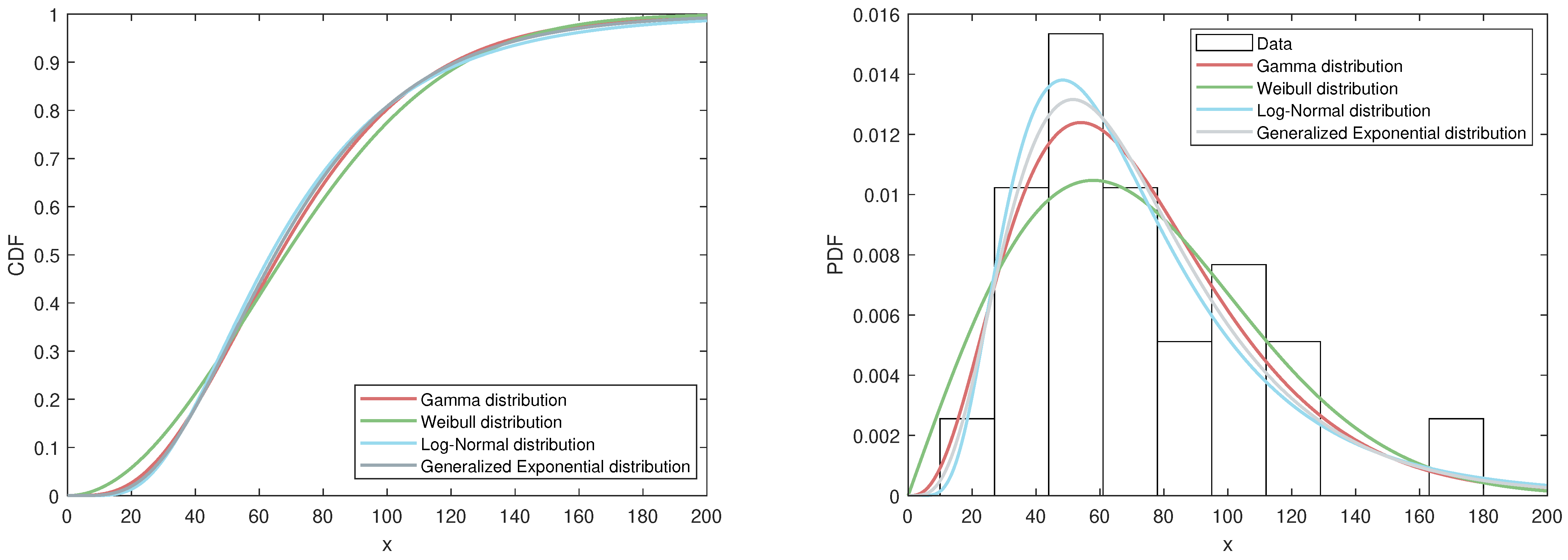
presents the test results for each distribution. Typically, better model fit is indicated by smaller values of K-S, A-D, AIC, and BIC, along with a higher log-likelihood value. As shown in the table, the generalized exponential distribution provides a good fit for this dataset. To further visualize the model performance, Figure 4 includes two plots based on the MLEs. The first plot compares the fitted CDFs of the four distributions mentioned above. The second plot displays the fitted PDFs of these four distributions alongside a histogram of the dataset.

Now, we consider the situation where the final three observations are censored, denoted as $r=20$. To estimate the unknown parameters, both Bayesian estimation and maximum likelihood estimation approaches are utilized. A summary of the estimation results is presented in

Table 12. Mean estimates of $\alpha$ and $\lambda$ for censoring scheme $n=23,r=20$ based on the real dataset.

Parameter	MLE	GELF		LILF		SELF
		$\mathit{\delta }=-\mathbf{0}.\mathbf{6}$	$\mathit{\delta }=\mathbf{0}.\mathbf{8}$	$\mathit{h}=-\mathbf{0}.\mathbf{2}$	$\mathit{h}=\mathbf{0}.\mathbf{6}$
$\alpha$	5.0439	5.0506	4.7649	5.3409	4.6706	5.1462
$\lambda$	0.0319	0.0297	0.0295	0.0301	0.0303	0.0287

.

The corresponding 95% asymptotic confidence intervals for $(\alpha ,\lambda )$ are $(2.5512,8.5386)$ and $(0.0225,0.0412)$, respectively. Meanwhile, the 95% HPD credible intervals are $(2.5123,6.4661)$ for $\alpha$ and $(0.0222,0.03426)$ for $\lambda$. Notably, the HPD intervals are shorter than the asymptotic confidence intervals.

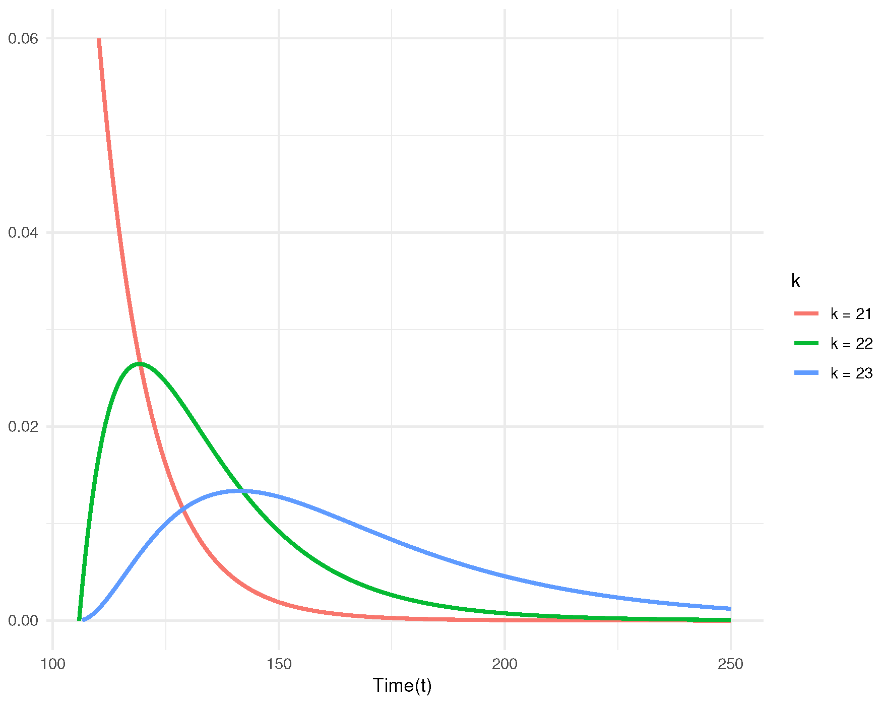
Now, we make predictive inference for the 21st, 22nd, and 23rd future order statistics, denoted as $X_{21}$, $X_{22}$, and $X_{23}$, using (41) and (44). We assume that the hyper-parameters are the same as in Section 5. From

Table 13. Point predictions and predictive intervals for $X_{21}$, $X_{22}$, and $X_{23}$ in the one-sample case.

k	True Value	Predictions	Intervals
21	127.92	119.1102	(106.1134, 147.1283)
22	128.04	138.6103	(109.4465, 194.0252)
23	173.40	176.8546	(118.7290, 289.9706)

, it is evident that the predicted values closely resemble the true values, thereby corroborating the effectiveness of our theoretical model. The Bayesian point prediction for the 21st order statistic is 127.92, with a 95% predictive interval ranging from 106.1134 to 147.1283. This suggests that, based on the observed sample, the 21st deep groove ball bearing is expected to fail between 106.11 and 147.13 million revolutions. 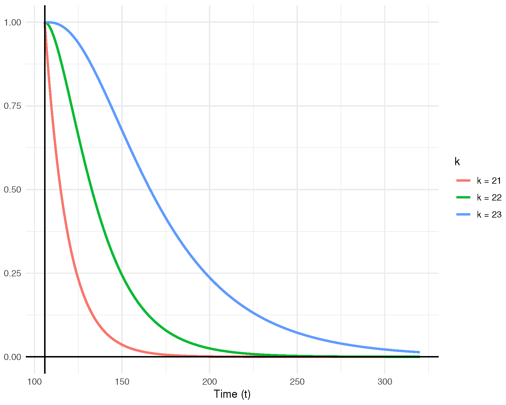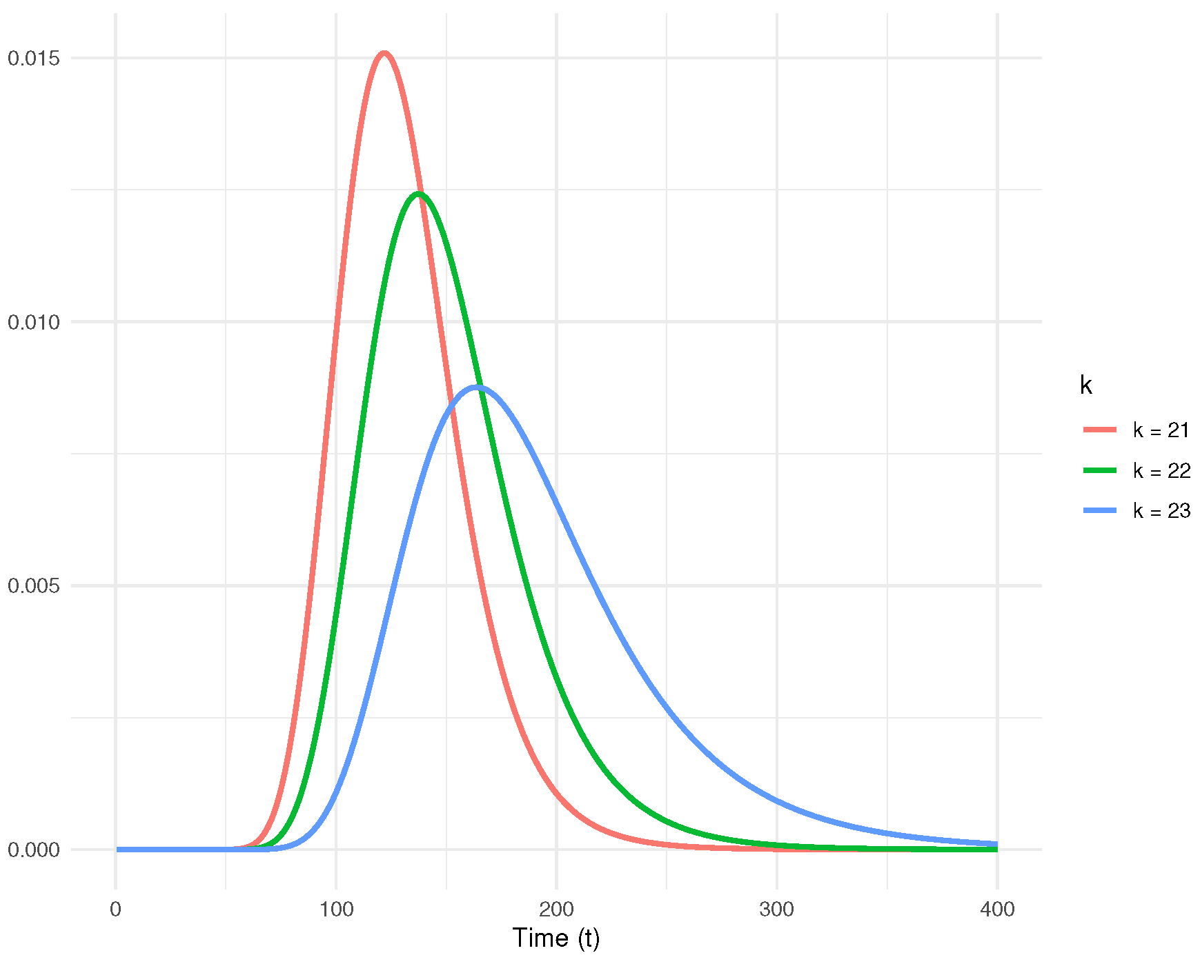Figure 5 illustrates the posterior predictive density functions for the censored observations. Additionally, the predictive survival functions for $X_{21}$, $X_{22}$, and $X_{23}$ are displayed in Figure 6. The plots clearly indicate that as k increases, the rate of decline in the predictive survival function decreases.

We now focus on the two-sample prediction problem discussed in Section 4.2. Assume 23 new deep groove ball bearings, denoted as $Y_1,Y_2,\dots ,Y_{23}$, are subjected to the same test. The goal is to derive the predictive density and make predictive inference for $Y_k$.

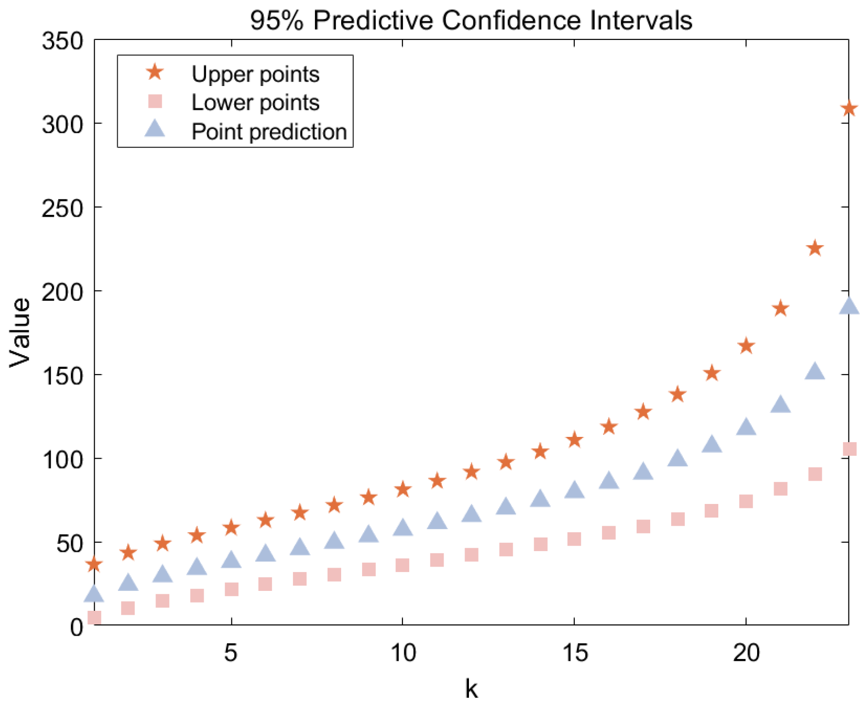
Figure 7 illustrates the point predictions and predictive intervals for the future samples derived from the observed dataset. Detailed numerical results are provided in

Table 14. Point predictions and predictive intervals in the two-sample case.

k	Point Prediction	Lower Bound	Upper Bound
1	17.6608	4.8729	36.4397
2	24.3465	10.2411	43.3671
3	29.4212	14.4497	48.8196
4	33.8348	18.0907	53.6814
5	37.9103	21.4086	58.2652
6	41.8053	24.5275	62.7310
7	45.6146	27.5226	67.1804
8	49.4043	30.4457	71.6893
9	53.2271	33.3365	76.3223
10	57.1294	36.2285	81.1406
11	61.1568	39.1524	86.2081
12	65.3576	42.1386	91.5963
13	69.7868	45.2195	97.3899
14	74.4534	48.4317	103.6955
15	79.6135	51.8191	110.6520
16	85.2072	55.4372	118.4508
17	90.6626	59.3598	127.3675
18	98.5624	63.6904	137.8241
19	106.9413	68.5841	150.5164
20	117.1294	74.2923	166.7142
21	130.6404	81.2710	189.1098
22	150.4528	90.5097	225.0417
23	189.4416	105.0678	308.4021

. The Bayesian point prediction for the median is 65.36, with a 95% predictive interval for the median ranging from 42.1386 to 91.5963. This suggests that, based on the observed sample, the 12th deep groove ball bearing is expected to fail between 42.14 and 91.60 million revolutions. The posterior predictive density functions for $Y_{21}$ to $Y_{23}$ are shown in Figure 8. It can be observed that as k increases, the expected values of $Y_k$ shift rightward, and the variances increase. 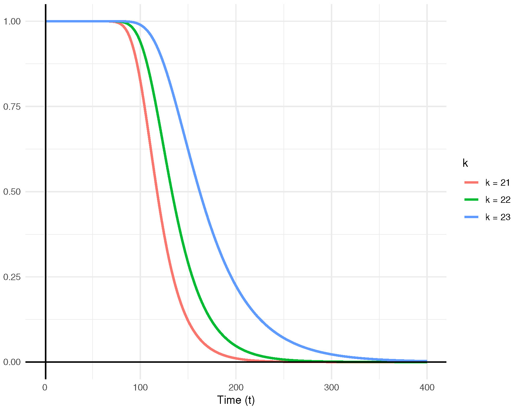Additionally, Figure 9 presents the predictive survival functions for $Y_{21}$, $Y_{22}$, and $Y_{23}$.

The results above, including both one-sample and two-sample predictions, can guide maintenance decisions by using the predictive intervals to schedule timely replacement or servicing of bearings, helping to prevent unexpected failures, minimize downtime, and reduce maintenance costs.

We encourage further research utilizing larger sample sizes and real-world datasets to achieve more accurate point and interval predictions, as well as to explore the impact of prior distribution selection on predictive outcomes.

7. Conclusions

In this study, we explore the estimation and prediction problems for the generalized exponential distribution based on Type-II censored data. The MLE is performed using the EM algorithm. Additionally, Bayesian estimation methods are investigated under various loss functions. Using Gibbs sampling and importance sampling, Bayesian estimates and HPD credible intervals are constructed. Monte Carlo simulations are conducted to assess and compare the performance of classical and Bayesian estimation techniques. Notably, the results indicate that Bayesian methods consistently provide lower MSEs and more precise interval estimates. For prediction, the proposed methods are applied to the endurance test data for deep groove ball bearings, where the last three observations are censored. Both one-sample and two-sample prediction scenarios are analyzed, with posterior predictive distributions used to construct predictive intervals. The findings demonstrate that Bayesian approaches offer a robust and reliable framework for both estimation and prediction in the presence of Type-II censored data.

One limitation of the Type-II censoring scheme is that units can only be censored at the final termination time. Future studies are encouraged to investigate more adaptable censoring schemes, such as progressive type-II hybrid censoring and adaptive Type-II progressive censoring. Moreover, exploring different prior distributions, alternative loss functions, or applying the model to other lifetime distributions could further improve the versatility and reliability of the approach.