Research on the Method of Calculating Anchorage Flaw Length Based on the Propagation Characteristics of Bolt Excitation Stress Waves

Abstract

This research aimed to detect the defects of anchoring agents’ empty slurries in anchor support. The influence of anchoring defects on the propagation law of stress waves was comprehensively investigated using laboratory tests, theoretical calculations, and other methods. The characteristic modal components with symmetry and periodicity laws were extracted by adopting a variable modal decomposition (VMD) signal decomposition method. It was found that the bottom reflection time of stress waves had an inverse function relationship with the length of the anchorage flaw. The average propagation speed of the stress wave in the free rod was obtained as 5150 m/s, and the average consolidation wave speed was 4198 m/s. The calculation method of the bolt flaw length was finally proposed. After experimental verification, the average error rate was 2.65%, which meets the requirement of testing accuracy in the engineering field, which provides a guarantee for safe production.

1. Introduction

Nowadays, anchor support technology is widely used in domestic and foreign countries, and it is one of the key technologies essential for coal mines to achieve high-yield and high-efficiency production. Anchor support can closely link the roadway surrounding rock with bolts and transmit the force on the surrounding rock through the bolts to maintain the stability of the roadway surrounding rock. The key to anchor support is to bond the surrounding rock to bolts through an anchoring agent [1,2,3]. However, due to the limitations of materials and engineering conditions, the anchoring system is bound to form a variety of anchoring defects such as the rusting of bolts, flaws in the empty slurry of anchors, and poor bonding effects of anchors with reinforcement materials and the surrounding rocks during construction and use. The existence of anchoring flaws reduces the bearing capacity of the anchoring system, which seriously causes the two sides of the roadway to move too close to each other, and accidents such as roofing ones seriously affect the safety of roadway support [4]. Therefore, domestic and foreign scholars have carried out a lot of research in anchorage quality detection, but there are still many shortcomings; most of this research only considered the length of bolts, the length of bolt solids, the location of flaws, and the detection of sound and lousy anchorage compactness, and for the length of flaws, less detection was conducted [5,6]. Research on the detection of bolt flaw length will help improve anchorage quality inspection and promote the development of anchorage quality inspection technology.

The quality inspection of bolt solid flaw detection technology is currently mainly based on nondestructive testing technology. Compared with conventional anchor pulling destructive anchoring quality inspection methods, nondestructive testing technology cannot damage or affect the use of the object under the premise of the performance of the object to be tested; using physical or chemical methods; with the help of advanced technology and equipment; the detection of defects within the object or on the surface; or the detection of defects, damages, inhomogeneity, and other issues, in order to ensure the object’s quality, safety, and reliability [7,8]. Vrkljan et al. [9] conducted vibration tests on anchors of different lengths in 1999, using small hammers to apply hammering loads at the top of the anchors and using accelerometers to receive the reflected signals of stress waves to study the relationship between the resonance frequency of the anchors and the anchorage length. Yi [10] transmitted and reflected waves using rules based on elastic stress wave propagation in grouted bolt solids. NDT experimental research was conducted on the free section of the grouted anchor bolt, the length of the bolt, and the location and length of the flaws within the anchor section to quantitatively determine the free section of the anchor bolt, the length of the bolt, and the specific location and length of the flaws within the anchor body. Zhu et al. [11] used ultrasonic-guided waves to detect the anchorage quality of anchorage flawed anchor rods. They used an improved adaptive noise complete ensemble empirical modal decomposition (CEEMD) method to analyze the ultrasonic-guided wave detection signals in anchored anchor rods to achieve the anchorage quality detection of the anchor rods and quantitative detection of the anchorage flaws in terms of the size of the anchor rods. Based on ultrasonic-guided wave nondestructive testing technology, Zhang et al. [12] studied the signals of defect-free and defect-containing anchored bolts, analyzed the propagation mechanism of guided waves in anchored bolts, and then detected the defects within the anchored body, which provided a reference for the evaluation of the anchoring quality of anchored bolts by using nondestructive testing technology. Numerous scholars have used the ultrasonic method [10], ultrasonic-guided wave method [11,12], and stress wave method [13,14,15,16,17,18] to study the anchorage quality and anchorage flaws in anchor rods, among which the stress wave nondestructive testing method has the advantages of fast transmission speed, long propagation distance, and sensitivity to the nature of the material, which is very suitable for the study of the defects of an empty slurry of an anchorage agent in an anchorage system.

The transmission law for stress waves in a bolt is affected by a number of factors. In Wang et al. [13], due to the resisting impact characteristics of anchored roadway supporting structures not being taken into full consideration in the existing mechanism of roadway dynamic failure, a dynamic analysis model of the bearing structure of rocks surrounding a mine roadway was built, and the dynamic action of P-waves was analyzed. Fan et al. [14] constructed an anchor solid model through finite element software to study stress wave propagation characteristics under different anchorage states and anchorage qualities; the stress wave propagation speed was negatively correlated with the density of the surrounding rock around the anchor bar, the stress wave amplitude did not have an exact attenuation speed in different rock formations, and denseness was significantly correlated with the reflective amplitude ratio of the bottom of the bar. Li et al. [15] found that a large number of joints contained in natural rock bodies significantly affected the propagation pattern of stress waves. The propagation of stress waves in the rock mass was accompanied by a decrease in amplitude and a decrease in wave speed. In this process, joints opened, closed, and slipped under the action of stress waves. Sun et al. [16] found that the stress wave velocity was closely related to the collaborative vibration and depended on the degree of bonding between the anchor body and the anchoring medium. The difference in the degree of bonding might be significant at different ages. Therefore, the bolt should not be considered a composite material when determining its wave velocity. Once the mortar had hardened, the synchronization of the stress waves increased, and the bolt could be considered a composite. Fun et al. [17] tested and analyzed the wave system characteristics of the bolt solid under the conditions of end anchorage and anchorage impaction from the point of view of the waveguide characteristics of the anchor solid. It was found that the propagation process of stress waves in resin bolt solid showed a certain periodic regularity. There was an approximate linear relationship between the wave velocity in the anchorage section and the anchorage compactness, based on which the waveguide characteristics could be inversely calculated to calculate the bolt’s characteristic length and the anchorage’s compactness. Niu et al. [18] investigated the stress wave propagation law in fully grouted rock anchors and flawed anchors and found that the velocity and amplitude attenuation of flawed anchored anchors were less than that of fully grouted rock anchors. The larger the flaw, the smaller the amplitude attenuation. In addition, amplitude attenuation increased with the distance of the flaw. Affected by the anchorage quality, the stress wave propagation law was highly complex, and some scholars had proposed that the anchorage flaws mainly affected the phase distribution, amplitude, energy change, and wave speed of the stress wave, where wave speed variations, in turn, directly affected the pole bottom reflected times.

Due to the influence of the complexity of rock engineering, the detected stress wave signals tended to behave in a more heterogeneous manner, resulting in difficulties in the identification of signals, such as time domain reflections at the bottom of the anchor and the location of the flaws. For this reason, Huang et al. [19] from NASA proposed empirical mode decomposition (EMD), which was different from the traditional Fourier transform; EMD was a technique applied to the analysis of nonstationary nonlinear signals, which removed the limitation of the Fourier transform, and had a better adaptability to the signal. It was also able to provide higher resolution. However, during the signal analysis, the empirical mode decomposition had endpoint effects and mode aliasing. In 2009, Huang et al. [20] proposed an improved algorithm for the problems of EMD, called ensemble empirical mode decomposition (EEMD), by adding the same level of Gaussian white noise to the original data and then performing EMD decomposition, and finally performing sum averaging, which could effectively eliminate the interference of noise. The effect was better than EMD in practical applications. In order to overcome the problems of significant reconstruction error and poor completeness of decomposition in EEMD, Torres et al. [21] proposed an improved EEMD algorithm by adding positive and negative pairs of auxiliary white noise to the original signal, which could be eliminated during ensemble averaging, and could be effectively used in EEMD. Phase cancellation during ensemble averaging can effectively improve the decomposition efficiency, thus forming the CEEMD. In order to better suppress the modal aliasing phenomenon of the EMD method, Dragomiretskiy et al. [22] proposed the VMD in 2014, which overcame the problems of endpoint effect and modal component aliasing of the EMD method and had a more solid mathematical theoretical foundation. Xu et al. [23] introduced the MF-VMD into analysis of bolt detection signals. MF-VMD was used to analyze the simulated vibration and bolt detection signals. The results showed that MF-VMD could effectively separate the eigenmode functions and eliminate noise interference even under substantial interference. Aiming at the problem that the noise interspersed with electromagnetic ultrasonic signals of the bolt significantly affected the extraction of useful information, Luo et al. [24] proposed a noise reduction method based on the cuckoo search algorithm, combining the variational modal decomposition and the independent component analysis to achieve the separation of the echo signal from the noise signal and to analyze the data of the bolt and the anchoring signal. Compared with the commonly used noise reduction methods, this method had better noise resistance and reduction effects. Li et al. [25] performed primary decomposition of the original detection signal or secondary decomposition of the eigenmode function by VMD signal analysis and processing method. Based on transmission characteristics of the excitation stress wave within the bolt, a bottom reflection time was also identified, and a method of calculating the anchorage length using the bottom reflection time was proposed. In summary, many scholars had adopted the VMD decomposition method for noise reduction in stress waves and had achieved many results that provided many practical bases for developing nondestructive testing technology for bolts.

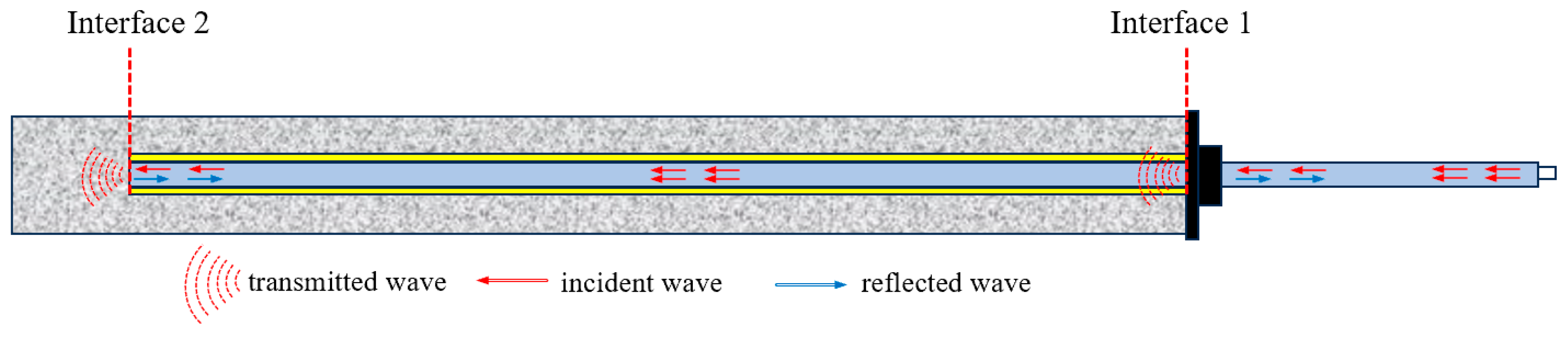
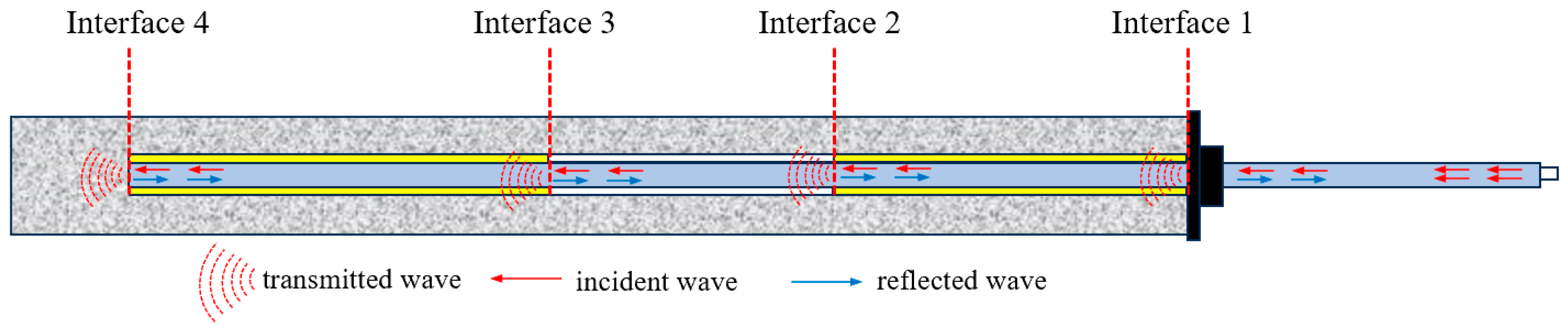
Presently, domestic and foreign experts have conducted detailed research on the propagation law of stress waves and have made many achievements. However, there are still some shortcomings due to the complexity of the composition of “anchors-resin anchors-anchor surrounding rock”. At present, it is still difficult to accurately describe the transmission law of stress waves in the anchorage system, and there are fewer studies on the anchorage flaws in the anchorage system. Therefore, it is essential to further investigate the significance of anchorage flaws within the law of stress wave propagation based on existing research, take the reflection of the stress wave at the bottom of the rod as the landing point, choose the appropriate stress wave signal processing method, and determine the length of the flaws through the propagation characteristics of the stress wave, to provide a valuable guideline for better implementation of nondestructive testing of anchor bars using the stress wave method.

2. Stress Wave Anchorage Flaw Detection Principle and Test System

2.1. Principle of Stress Wave Anchorage Flaw Detection

Numerous studies have shown that the physical properties of the medium itself mainly determine the propagation speed of stress waves in a medium. The stress wave emitted from the end of the bolt propagates inwards through the body of the bolt, and when it encounters the interface with the difference in wave impedance, reflection and transmission will occur. When the stress wave is transmitted to the bottom of the bolt, due to the apparent difference between the wave impedance of the anchor and the surrounding rock, there is an obvious reflection of the stress wave, and this propagation law can be applied to the detection of flaws in the anchor. As shown in Figure 1, when there is no flaw in the bolt solid, the transmission and reflection of stress waves only occur at the port and bottom of the bolt solid. In the former case, under the influence of anchorage holding force, there is a slight change in wave impedance at the interface between the bolt and the anchorage, which produces a weak reflection phenomenon and has a weak influence on the transmission of the stress waves. The latter stress wave is transmitted from the bolt into the surrounding rocks; due to the huge difference between the bolt and the surrounding rocks in physical properties and structural composition, the stress wave forms obvious transmission and reflection phenomena, which is called bottom reflection.

However, under conventional circumstances, the anchoring agent cannot fill the borehole, and a cavity flaw will be formed in a particular region of the anchoring section, affecting anchoring quality. As shown in Figure 2, if a cavity is formed inside a bolt solid, the stress wave propagating inside the bolt will pass through four wave impedance change interfaces, such as interface 1 to interface 4, in sequence. When the stress wave propagates to interface 1 by the anchor holding force, the wave impedance of the anchored section of the bolt changes, and the speed of the stress wave also changes. When the stress wave passes through interface 2, the stress wave is incident to the light bar from the anchorage section, the interface wave impedance changes, and the interface undergoes stress wave refraction and transmission phenomena. Similarly, when the stress wave reaches interface 3, the interface will again experience stress wave refraction and transmission. When the stress wave reaches interface 4, the stress wave is transmitted from the bolt into the surrounding rock; due to the vast difference between the anchor bolt and the surrounding rock in terms of physical properties and structural composition, the change in wave impedance at the interface is pronounced. The stress wave will form apparent transmission and reflection phenomena, generating the bottom-end reflection. When the bottom reflection signal is transmitted back to the end, the stress wave will pass through interface 3 to interface 1, and the transmission and reflection phenomena will occur again. Therefore, the stress wave undergoes at least six interface reflections and one bottom reflection in a complete propagation cycle.

Ideally, the stress waves are reflected as they pass through interfaces 2 and 3 accordingly. Suppose the arrival time of the respective reflection signals can be extracted. In that case, the time difference can be used to calculate the position of interface 2 and interface 3 and the specific length of the cavity region. However, in the actual signal measurement and analysis, it was found that the transmission and reflection phenomena of interface 2 and interface 3 were highly complex, and it was difficult to monitor them directly by conventional means, so it was impossible to analyze the location of the anchorage flaws. Therefore, we can only use an indirect method to calculate the bolt flaw length through the periodic change rule of the reflected signal at the bottom of the stress wave. Figure 3 shows a plot of the original stress wave signals collected from the flawed bolt solid. Due to the multiple modal superposition of reflected and transmitted waves, the stress waveform is highly complex, and it is impossible to extract the bottom reflection signal directly from the original waveform, so it is necessary to take appropriate signal processing methods to decompose the stress wave.

2.2. Principle of VMD Decomposition

Current signal processing methods are mainly divided into EMD and VMD. Compared with the traditional time–frequency analysis techniques, EMD does not need to choose the basis function, which overcomes the problem that the basis function is not adaptive in the wavelet transform, and its decomposition is based on the distribution of the extreme points of the signal itself. However, there are two flaws in using the EMD method: the phenomenon of modal superposition and the endpoint effect. Therefore, some scholars have proposed EMD-like signal decomposition methods on this basis to try to solve the problems of EMD methods but achieved little success.

Unlike the EMD principle, the VMD decomposition method uses an iterative search for the optimal solution of the variational model to determine the center frequencies and bandwidths of the components of each decomposition and is an entirely nonrecursive model. It overcomes the problems of endpoint effects and modal component aliasing of the EMD method and has better results for processing nonlinear nonsmooth signals. The VMD decomposition method has two significant effects: (1) it can denoise the original detection signal containing noise, and (2) the decomposition of the denoised signal can obtain the modal components with bottom reflection characteristics. Therefore, in this paper, VMD is considered comprehensively for noise reduction in stress wave signals.

The VMD decomposition consists of two main parts, the construction of the signal and the solution, and the steps are as follows:

Denote the original signal to be decomposed as $x\left(t\right)$, where $t$ denotes time. Decompose the original signal into a number of IMF component signals $uk\left(t\right)$; $k$ denotes the number of eigenmode functions obtained after decomposition, and each IMF component can be used as a set of amplitude–frequency signals:

$$uk\left(t\right)=\mathrm{R}\mathrm{e}\left\{Ak\left(t\right)\times e^{iBk\left(t\right)})\right\}$$

(1)

where $uk\left(t\right)=\left\{u_1,u_2,\cdot \cdot \cdot ,u_k\right\}$ denotes the set of each IMF component of the decomposition, $\mathrm{R}\mathrm{e}\left\{\right\}$ denotes the real part taken, and $Ak\left(t\right)$ and $Bk\left(t\right)$ denote the amplitude and phase of the signal, respectively;

The Hilbert transform is applied to each IMF component to obtain the analytical signal and one-sided spectrum of each modal component, and the results are as follows:

$$\left(\delta (t)+{\displaystyle \frac{j}{\pi t}}\right)\times uk(t)$$

(2)

where $\delta \left(t\right)$ is the unit impulse function, $\times$ is the convolution operation, and $j$ is the imaginary unit.

An exponential parameter $e^{-j{\omega }_k\left(t\right)}$ is introduced to correct the center frequency of each modal component, shifting the spectrum of each modal function to its corresponding fundamental frequency band:

$$\left[\left(\delta (t)+{\displaystyle \frac{j}{\pi t}}\right)\times uk(t)\right]e^{-j{\omega }_k\left(t\right)}$$

(3)

where ${\omega }_k\left(t\right)$ is the set of center frequencies, ${\omega }_k\left(t\right)=B_k{\left(t\right)}^{\prime }$.

The signal is then demodulated by Gaussian smoothing to obtain the bandwidth description of each modal function, and the computational model is as follows:

$$\underset{\left\{u_k,{\omega }_k\right\}}{\mathrm{m}\mathrm{i}\mathrm{n}}\left\{\sum _{k=1}^k{‖\partial (t)\left[\left(\delta (t)+{\displaystyle \frac{j}{\pi t}}\right)\times uk(t)\right]e^{-j{\omega }_k\left(t\right)}‖}_2^2\right\}$$

(4)

$$s.t.\sum _{k=1}^k{u}_k\left(t\right)=x\left(t\right)$$

(5)

where $\partial \left(t\right)$ is to find the partial derivative.

The constrained variational problem is converted into an unconstrained variational problem by introducing Lagrange multipliers $\lambda$ and quadratic penalty factors $\alpha$ based on the above formulation, and the transformation results are as follows:

$$\begin{array}{c}L(\left\{u_k\right\},\left\{{\omega }_k\right\},\lambda )=\alpha {\displaystyle \sum _{k=1}^k}{‖\partial (t)\left[\left(\delta (t)+{\displaystyle \frac{j}{\pi t}}\right)\times uk(t)\right]e^{-j{\omega }_k\left(t\right)}‖}_2^2+\\ {‖f(t)-{\displaystyle \sum _{k=1}^k}{u}_k(t)‖}_2^2+〈\lambda (t),f(t)-{\displaystyle \sum _{k=1}^k}{u}_k\left(t\right)〉\end{array}$$

(6)

Finally, the main variables in the above equations are iteratively updated by the alternating multiplier operator to obtain the optimal modal components, center frequencies, and Lagrange multipliers, and the updated equations for the optimal modal components $u_k^{n+1}\left(\omega \right)$ are as follows:

$$u_k^{n+1}(\omega )={\displaystyle \frac{\widehat{f}\left(\omega \right)-\sum _{i<k}{{\widehat{u}}_i}^{n+1}\left(\omega \right)-\sum _{i>k}{{\widehat{u}}_i}^{n+1}\left(\omega \right)+\frac{{\widehat{\lambda }}^n\left(\omega \right)}{2}}{1+2\alpha {(\omega -{{\omega }_k}^n)}^2}}$$

(7)

At the end of each iterative update of the IMF components, the center frequency ${\omega }_k^{n+1}$ and the Lagrange multipliers $\lambda$ are updated with the following equations:

$${{\omega }_k}^{n+1}={\displaystyle \frac{{\int }_0^{\infty }\omega {\left|{{\widehat{u}}_k}^{n+1}(\omega )\right|}^{2}d\omega }{{\int }_0^{\infty }{\left|{{\widehat{u}}_k}^{n+1}(\omega )\right|}^{2}d\omega }}$$

(8)

$${\widehat{\lambda }}^{n+1}(\omega )={\widehat{\lambda }}^n(\omega )+\tau (\widehat{f}(\omega )-\sum _{i=1}^{k-1}{{\widehat{u}}_i}^{n+1}(\omega ))$$

(9)

In the formula, ^{^} is the Fourier transform, $n$ is the number of iterations, and $\tau$ is the fidelity coefficient.

The termination conditions for the iterative update of the above equation are as follows:

$$\sum _{k=1}^k\left({‖{{\widehat{u}}_k}^{n+1}(\omega )-{{\widehat{u}}_k}^n(\omega )‖}_2^2/{‖{{\widehat{u}}_k}^n(\omega )‖}_2^2\right)<\epsilon$$

(10)

In summary, the ultimate goal of VMD decomposition is to decompose the original detected signal into intrinsic modal components with their respective center frequencies and bandwidths, i.e., IMF components. Thus, the frequency and bandwidth of the signal are redivided effectively to ensure that each modal component contains its own signal characteristics, and the decomposition flowchart is shown in Figure 4.

2.3. Test System Construction

2.3.1. Experimental Programme

In order to study the influence of different flaw lengths on the NDT signal characteristics and its indicators in the full-length bolt solid system, six anchor solid specimens with different types of anchorage flaw lengths were fabricated in the anchor solid, respectively, MG1~MG6. In order to control the relatively fixed location of the anchorage flaws and to facilitate the signal analysis, the specimen flaw location was ensured to be in the middle of the borehole as far as possible and to maintain a symmetrical distribution at both ends. The specimen dimensions are shown in Figure 5. The specimen parameters are shown in

Table 1. Parameter table of bolt solid specimens with different bolt flaw lengths.

Model Number	Anchor Length (mm)	Exposed Length (mm)	Length of Flawed Section (mm)
MG1-1–MG1-3	900	300	0
MG2-1–MG2-3	900	300	50
MG3-1–MG3-3	900	300	100
MG4-1–MG4-3	900	300	150
MG5-1–MG5-3	900	300	200
MG6-1–MG6-3	0	300	900

. In order to ensure the reliability of the samples, three specimens of each type of flaw length of bolt solid were produced. The lengths of empty slurry flaws of the specimens of the MG1~MG6 series were in this order: 0 mm (full anchor), 50 mm, 100 mm, 150 mm, 200 mm, and 900 mm (free anchor bar). The free end of the bolt is 300 mm long. After the specimens are made, the wireless anchor quality detector collects signals from each specimen.

2.3.2. Test Piece Production

The anchor bolts used in the NDT experiments were Q335 left-hand threaded steel anchors. The surrounding rock was simulated by mortar, the calculation ratio was water: cement: sand = 1:2:4 for the medium stability rock layer commonly found in the roadway, and the average compressive strength of the surrounding rock was 37.65 MPa after the standard compression test, which meets the requirements of the experiment. According to the mixing ratio, 21 columnar mortar specimens were made, and 32 mm diameter drill holes were reserved in the center of the specimens [26,27]. After the mortar had solidified, they were placed vertically for 28 d. The anchoring was carried out after the maintenance was completed according to the experimental plan. The completed specimens are shown in Figure 6.

2.3.3. Signal Acquisition

The wireless anchor quality tester used is shown in Figure 7. It was based on Wi-Fi wireless data transmission, and the test host input pulsed high voltage into the roller shaker, generating an alternating magnetic field, which drove the self-excited vibration of the rod in the roller shaker. Stress wave method testing has the advantages of fast propagation speed, long propagation distance, and simple operation. The following issues need to be noted when using the anchor nondestructive testing instrument to collect signals:

(1)

The leveling of the end of the measuring rod and the installation of the sensor:

First, we used a steel file to polish the top of the measuring rod flat, and then we used an electric drill to drill an eye in the middle of the end of the measuring rod to install the acceleration sensor. When installing the acceleration sensor, in order to ensure the objectivity of the test results, two factors should be considered:

The installation position and direction of the sensor. As the propagation law of elastic stress wave was based on the one-dimensional longitudinal wave propagation theory, the axis of the sensor had to be parallel to the axis of the measuring rod. Otherwise, the angle between the incident wave and the reflected wave would be generated (phase difference), and the two-dimensional effect was challenging to overcome.

The coupling between the sensor and the top of the measuring rod was critical. If the installation was not careful, it would cause parasitic oscillations; if the bonding state is not good, it will reduce the resonant frequency of the sensor installation, and in severe cases, it will restrict the effective use of the acceleration sensor range so that the test failed. Therefore, in the experiment, the effect of using a petroleum-jelly-coated anchor rod head was good.

(2)

Signal acquisition parameter setting:

The signal acquisition process needed to debug the parameters of nondestructive testing; signal acquisition parameter settings mainly included the sampling rate, the number of sampling points, channel gain, and emission energy adjustment to collect the appropriate signal amplitude. In order to ensure the accuracy of signal acquisition and the acquisition of multiple stress wave signal propagation cycles, we needed to reduce the sampling time interval and increase the number of sampling points per unit of time, and the sample frequency Fs had to be greater than the highest frequency of the components of the signal under test Fm twice. According to experience, the final sampling rate was set to the maximum sampling rate of 1 MHz, the number of sampling time points was set to 6k, and the channel gain and launch energy adjustment of the two were used in conjunction with each other; the greater the gain, the greater the signal amplitude, and the greater the launch energy of the signal amplitude. But if the launch energy was too large, the rod head would produce aftershocks and interference with typical signal acquisition. In the signal acquisition process for each group of specimens, to ensure the stability and reliability of the detection signal, each specimen was acquired three times; each acquisition contained three groups of signals, and a total of nine groups of data were acquired.

3. Analysis of Test Results

3.1. MG1 Series Specimen Detection Signal Analysis

The results of MG1-1 decomposition using VMD are shown in Figure 8. The original detection signal is decomposed into eight modal function component signals. The former seven modal components of the rod bottom reflection and periodicity are not prominent and play little role in determining the rod bottom reflection time. Observation of the IMF8 component signal in Figure 9 reveals that the component waveform has an obvious symmetry and periodic decay pattern. The waveform graph shows multiple peaks and multiple reflections at the bottom of the pole, which is referred to as the eigenmode component in this paper. The time interval between adjacent peaks is the time it takes for the stress waves to make a round trip within a bolt, referred to here as bottom reflection time. In order to reduce the calculation error of the bottom reflection time, this paper takes the average value of the time difference between several adjacent peaks in the eigenmodal component as the bottom reflection time. Finally, it determines that the bottom reflection time of the specimen is 545.5 μs.

For the same three specimens without anchorage flaws, nine sets of data collected from each specimen were processed as described above. The average value of the bottom reflection time for each specimen was calculated, and the results of the calculations are shown in

Table 2. Specimen MG1 series specimen rod bottom reflection time.

Specimen Number	Length of Exposed Section of Bolt/mm	Actual Anchorage Length/mm	Average Rod Bottom Reflection Time/μs
MG1-1	301	899	546.1
MG1-2	303	897	543.7
MG1-3	300	900	545.8

.

3.2. MG2 Series Specimen Detection Signal Analysis

The above VMD decomposition was performed on the detection signal of the specimen with MG2-1, and the decomposition results are shown in Figure 10. When analyzing the IMF3 and IMF8 components in Figure 11, it can be found that these two modal component signals have multiple reflections from the bottom of the rod, the time interval between adjacent peaks is the same, and the periodicity and symmetry are apparent, which are the characteristic modal components. After calculation, the average rod bottom reflection time was 541.1 μs. For the three specimens with 5 cm flaws, 9 datasets collected from each specimen were processed as above. The average value of the bottom reflection time for each specimen was calculated, and the calculation results are shown in

Table 3. Specimen MG2 series specimen rod bottom reflection time.

Specimen Number	Length of Exposed Section of Bolt/mm	Actual Anchorage Length/mm	Average Rod Bottom Reflection Time/μs
MG2-1	305	895	540.2
MG2-2	303	897	540.7
MG2-3	299	901	541.3

.

3.3. MG3 Series Specimen Detection Signal Analysis

The decomposition results of the MG3-1 specimen are shown in Figure 12. The rod bottom reflection signals can be seen in both IMF5 and IMF7 modal component signals in Figure 13. The signal in the IMF7 modal component is relatively smooth, with a symmetric and periodic decay pattern. The time intervals between neighboring crests are essentially the same. When observing the signal of the IMF5 modal component, it is found that a signal with a smaller amplitude is superimposed between two adjacent wave peaks with a larger amplitude, and it is inferred that the signal may be the reflection signal formed by the reflection phenomenon of the stress wave propagating to the flaw location in the bolt. Since the change in wave impedance at the flaw location is smaller than that at the bottom of the bolt, only part of the propagation direction of the stress wave is changed, the energy of the reflected wave is relatively weak, and the amplitude of the decomposed modal component signal is relatively small.

The IMF5 modal component signal will inevitably affect the determination of the reflection time T at the bottom of the rod due to the superposition of the reflection signal at the location of the flaw. In order to remove the superposition of the reflection signal at the flaw location, this paper carries out a secondary decomposition of the IMF5 modal component signal, i.e., the IMF5 modal component signal is processed by the variational modal decomposition (VMD), and the decomposition results are shown in Figure 14: the secondary decomposition results of IMF1, IMF2, IMF3, IMF5, and IMF8 all show multiple rod bottom reflections, with apparent symmetry and periodicity patterns, for the desired eigenmode components. The time difference between adjacent wave peaks was taken as a rod bottom reflection time, the average value of multiple rod bottom reflection times was calculated, and the average value of rod bottom reflection time was finally obtained as 536.3 μs.

The above treatment was performed for all three specimens with all the flaw lengths of 150 mm, and the bottom reflection times obtained for each bolt are shown in

Table 4. Specimen MG3 series specimen rod bottom reflection time.

Specimen Number	Length of Exposed Section of Bolt/mm	Actual Anchorage Length/mm	Average Rod Bottom Reflection Time/μs
MG3-1	302	898	536.0
MG3-2	300	900	535.8
MG3-3	299	901	536.2

below.

3.4. MG4 Series Specimen Detection Signal Analysis

The decomposition of the time domain signal of the MG4-1 specimen yielded eight modal components, as shown in Figure 15, and the denseness of the signal reflects the frequencies of the different modal components, which are different from each other. From Figure 16, it can be seen that the IMF8 component signal rod bottom reflection is clear, symmetry and periodicity are obvious, and there is basically no reflection signal superposition for the characteristic modal component signal. By calculating the time difference between adjacent peaks in the IMF8 edge component signal and calculating the average value, the rod bottom reflection time was obtained as 531.8 μs.

The nine sets of data collected from each of the three specimens with the same length of anchorage flaws were processed according to the above procedure to find the bottom reflection time for each specimen. The obtained bottom reflection times for each rod are shown in

Table 5. Specimen MG4 series specimen rod bottom reflection time.

Specimen Number	Length of Exposed Section of Bolt/mm	Actual Anchorage Length/mm	Average Rod Bottom Reflection Time/μs
MG4-1	300	900	532.6
MG4-2	302	898	531.3
MG4-3	301	899	531.0

below.

3.5. MG5 Series Specimen Detection Signal Analysis

As shown in Figure 17, the time domain signal detected by specimen MG5-1 is decomposed into eight modal function component signals. Among them, IMF2, IMF5, and IMF6 in Figure 18 are the eigenmodal component signals. The eigenmodal components have multiple symmetrical and periodic waveform decay features, and the reflection signals at the bottom of the rod are apparent. Therefore, we calculated the time difference between adjacent peaks of the three components and found the average value, which was taken as the bottom reflection time for the bolt. We found the average bottom reflection time for the bolt to be 528.7 μs.

The nine datasets collected from each of the three specimens with the same flaw length were processed as above. The time difference between the crest points in the eigenmode function components was calculated to obtain the average bolt bottom reflection time.

Table 6. Specimen MG5 series specimen rod bottom reflection time.

Specimen Number	Length of Exposed Section of Bolt/mm	Actual Anchorage Length/mm	Average Rod Bottom Reflection Time/μs
MG5-1	298	902	529.1
MG5-2	297	903	528.2
MG5-3	301	899	526.3

shows the bolt bottom reflection time for each rod of the MG5 model.

3.6. MG6 Series Specimen Detection Signal Analysis

As shown in Figure 19 for the test signal of specimen MG6-1 after VMD decomposition, it can be clearly seen that there are symmetrical and periodic waveforms in each component, and the reflection at the bottom of the rod is clear. The peak value of the waveform in each component signal was selected, and the difference between adjacent peaks was taken as a rod bottom reflection time; the average rod bottom time of each component was calculated, and, finally, the average value of the rod bottom reflection time of eight components was taken. The final rod bottom reflection time was 466.3 μs.

Nine sets of data collected for each of the three specimens of the same length were processed as described above, and the following

Table 7. Specimen MG6 series specimen rod bottom reflection time.

Specimen Number	Length of Exposed Section of Bolt/mm	Actual Anchorage Length/mm	Average Rod Bottom Reflection Time/μs
MG6-1	299	0	466.2
MG6-2	301	0	465.7
MG6-3	300	0	466.1

shows the bottom reflection time for each specimen.

By performing VMD decomposition of the detected stress wave signals of specimens with different anchorage flaw lengths and in-depth analyses of the obtained eigenmode signals, the rod bottom reflection time of each specimen was determined from them. The results of the analyses show that the rod bottom reflection time gradually decreases with the increase in the anchorage flaw length. This trend indicates that the propagation speed of stress waves in the anchor rods decreases when the anchors are in the anchored state, which may be because there is a holding force between the anchoring agent and the anchor rods in the anchored state compared to the free anchors, resulting in a reduction in the propagation speed of the stress waves in the anchored section of the anchor rods. Therefore, the longer the anchorage flaw in the anchorage system, the shorter the time for the stress wave to propagate one cycle in the anchor.

4. Calculation Method and Validation of Anchorage Flaw Length Based on the Propagation Characteristics of Excited Reflected Stress Wave

4.1. Calculation of the Length of an Anchorage Flaw

The above studies show that flaws in the anchoring system affect the bottom reflection time of stress waves in anchors, as shown by the fact that the bottom reflection time becomes shorter as the length of the flaw increases. This phenomenon is due to the difference in the propagation speed of stress waves in different media. As a result, after a stress wave is excited within the bolt end, the stress waves travel along the bolt to the bottom of the bolt and then from the bottom of the bolt back to the head of the bolt. Due to the different propagation speeds of the stress wave in different media, the time spent in the process of propagating to the bottom of the rod and returning to the head of the rod from the bottom of the rod is not the same. This time difference will change with the different defects in the anchoring system. When the defect length is larger, the impact of the stress wave propagation process is greater, which makes the bottom reflection time shorter, and accordingly the whole propagation process will take a different time to the normal situation. According to the principle of stress wave propagation, the time taken by the stress wave in the anchorage system to propagate one round trip in the anchor is composed of the following three parts: (1) stress wave propagation time $T_1$ in the exposed section of the anchor, (2) stress wave propagation time $T_2$ in the dense section of the anchor, and (3) stress wave propagation time $T_3$ in the defective section of the empty slurry of the anchor. The reflection time course of the bottom of the rod in the anchoring system can be expressed as Formula (11):

$$T=T_1+T_2+T_3={\displaystyle \frac{2l_e}{c}}+{\displaystyle \frac{2l_d}{V_d}}+{\displaystyle \frac{2(l-l_e-l_d)}{V}}$$

(11)

According to the above equation, it can be obtained that the length of the flawed section in the anchoring system can be calculated by Equation (12):

$$l_d={\displaystyle \frac{V_d(TCV-2V{l}_e-2Cl+2C{l}_e)}{2C(V-V_d)}}$$

(12)

where $l$ is the length of the anchor rod, $l_e$ is the length of the exposed section of the anchor rod, which can be directly measured in the experiment; $l_d$ is the length of the defective section of the empty slurry, $C$ is the propagation speed of the stress wave in the free rod, $V$ is the velocity of the consolidation wave, $V_d$ is the propagation speed of the stress wave in the flawed section, and $T$ is the time used for the propagation of the stress wave in the anchor rod for one round trip. Therefore, to accurately calculate the length of the anchorage trap section in the anchorage system, we first need to calculate the size of $C$, $V$, and $T$.

(1)

Determination of free rod wave velocity ($C$):

The velocity $C$ of the stress wave propagating in the free rod can be determined from Equation (13).

$$C={\displaystyle \frac{2l}{T}}$$

(13)

where l is the length of the anchor rod (1200 mm), and $T$ is the reflection time at the bottom of the rod for the MG6 specimen. The wave speeds $C$ of the three free rods were obtained as 5148 m/s, 5153 m/s, and 5149 m/s, respectively, and these calculations were averaged to finally determine the size of $C$ as 5150 m/s.

(2)

Determination of consolidation wave velocity $V$:

Regarding the determination of consolidation wave velocity $V$, the study object is mainly for specimens without anchorage flaws. The bottom reflection time consists of two parts: the propagation time of the stress wave in the exposed section of the anchor $T_w$, as well as the propagation time of the anchorage section $T_m$, which can be expressed as follows:

$$T=T_w+T_m={\displaystyle \frac{2l_e}{c}}+{\displaystyle \frac{2(l-l_e)}{V}}$$

(14)

Then the consolidation wave velocity $V$ can be expressed as

$$V={\displaystyle \frac{2C(l-l_e)}{CT-2l_e}}$$

(15)

where, for the bottom reflection time of the above MG1 specimen, the consolidation wave velocity $V$ in the three flawless anchorage specimens was calculated to be 4189 m/s, 4211 m/s, and 4193 m/s, respectively, and the average value was taken to determine $V$ as 4198 m/s.

(3)

Determination of stress wave propagation velocity $V_d$ in anchorage flaw section

In the experiment of making specimens with anchorage flaws, to determine the existence of anchorage flaws inside the bolt solid, the made specimens were crushed. Figure 20 below shows the remaining anchor rods stained with an anchoring agent after crushing the specimens with anchorage flaws.

From the figure, it can be seen that there are anchorage flaws inside the red frame line. After careful observation, it was found that a thin layer of anchoring agent was attached to the surface of the defective section of anchor rods. Therefore, in order to determine the transmission speed of the stress waves in the flawed section of the anchorage system, three anchor rods with a length of 1200 mm and an anchoring agent attached to the surface were fabricated and labeled as M1, M2, and M3, respectively, and the fabricated rods are shown in Figure 21.

The anchor quality tester detected the bolt excitation stress wave on three anchor rods, as shown in Figure 22. The signal maps were obtained after denoising the detected signals. The comparison found that the time domain signal plots of the attached anchored anchor rods and the free rods were nearly the same. We calculated the bottom reflection time for the detection signals of M1, M2, and M3 anchor rods. The bottom reflection time was 466.4 μs, 466.1 μs, and 465.6 μs, respectively. The transmission speeds of the stress waves within M1, M2, and M3 bolts were obtained to be 5146 m/s, 5149 m/s, and 5155 m/s according to the formulae, and in order to obtain more representative data, we took the wave speeds of the three specimens as the average value to obtain $V_d=C=5150$ m/s. Therefore, Equation (12) can be simplified as follows:

$$l_d={\displaystyle \frac{2Cl+2V{l}_e-CV-2C{l}_e}{2(C-V)}}$$

(16)

4.2. Experimental Verification of the Length of Anchorage Flaws

To confirm the accuracy and feasibility, we calculated the anchorage flaw length. Strictly following the content of Section 2.3.2., three new anchor anchorage specimens, labeled YZ1, YZ2, and YZ3, were prepared, and the location and length of flaws in these three specimens were randomly set. Then, the specimens were subjected to stress wave nondestructive testing, as shown in Figure 23; the three specimens were inspected in the field during the verification test.

After the signal acquisition was completed, the acquired stress wave signals were decomposed by the VMD signal processing method, and the characteristic modal signals with obvious reflection signals at the bottom end were searched for in each modal signal after decomposition. If the reflection signal of the flaw location was superimposed in the eigenmode signal, the secondary decomposition was carried out. The components with apparent symmetry and periodicity in the secondary decomposition were extracted as the characteristic modal signals, and the average bottom reflection time of the specimen was calculated sequentially. The length of the anchorage flaw segment in the anchored specimen was then calculated according to the formula established above. Finally, the specimen was broken, and the actual anchorage flaw segment length inside the specimen was measured to calculate the error in the stress wave detection results. Figure 24 shows the flow chart of the validation experiment.

The characteristic modal signals after the decomposition of each detection signal were analyzed, and the reflection times at the bottom of the rod corresponding to specimens YZ1, YZ2, and YZ3 were determined to be 529.7 μs, 534.9 μs, and 539.1 μs, respectively. According to equation, the lengths of anchorage flaws in the three specimens were calculated to be 174.9 mm, 118.9 mm, and 70.1 mm. Subsequently, the three specimens were then crushed, and the results after crushing are shown in Figure 25.

Observation of the figure reveals that after the resin anchorage had been set, the material brittleness increased significantly due to the material’s brittleness. When the specimen was broken, the integrity of the anchorage itself suffered a certain degree of damage. This is manifested by the fact that part of the anchoring agent was attached to the anchor rods while the other was attached to the surrounding rock. In areas where the anchorage was flawed, the integrity of the anchorage remained intact, with a relatively thin layer of anchorage attached to the anchor rods. A rigid ruler was used to measure the anchorage flaws, as shown in the figure for the field measurement; the lengths of the flaws inside the three specimens were about 178.2 mm, 117.0 mm, and 67.1 mm. The validation experimental test results and the actual test results and errors are shown in

Table 8. Verification of experimental test results and errors.

Specimen Number	Exposed Length of Bolt (mm)	Anchorage Flaw Detection Results (mm)	Actual Measurement (mm)	Difference (mm)	Detection Error (%)
YZ1	302	174.9	178.2	3.3	1.85%
YZ2	299	118.9	117.0	1.9	1.62%
YZ3	300	70.1	67.1	3.0	4.47%

.

Table 8 shows the detection results of the maximum and minimum differences of 3.3 mm and 1.9 mm, respectively, with an average difference of 2.7 mm. The detection error of the maximum and minimum values of 4.47% and 1.62%, respectively, was the average error of 2.65%. Overall, the stress wave detection results are consistent with the actual measurement results, and the detection error is small and stable. The results show that using the bottom reflection time of the stress waves detection signal to judge the length of the anchorage flaw is feasible.

5. Conclusions

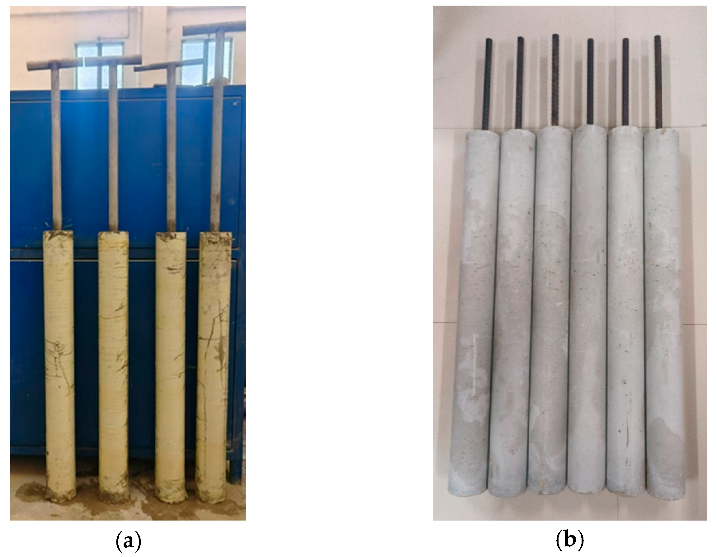
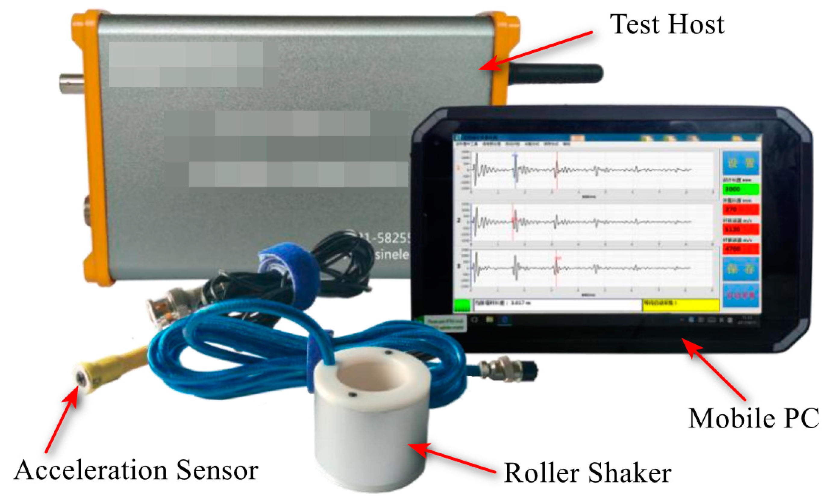
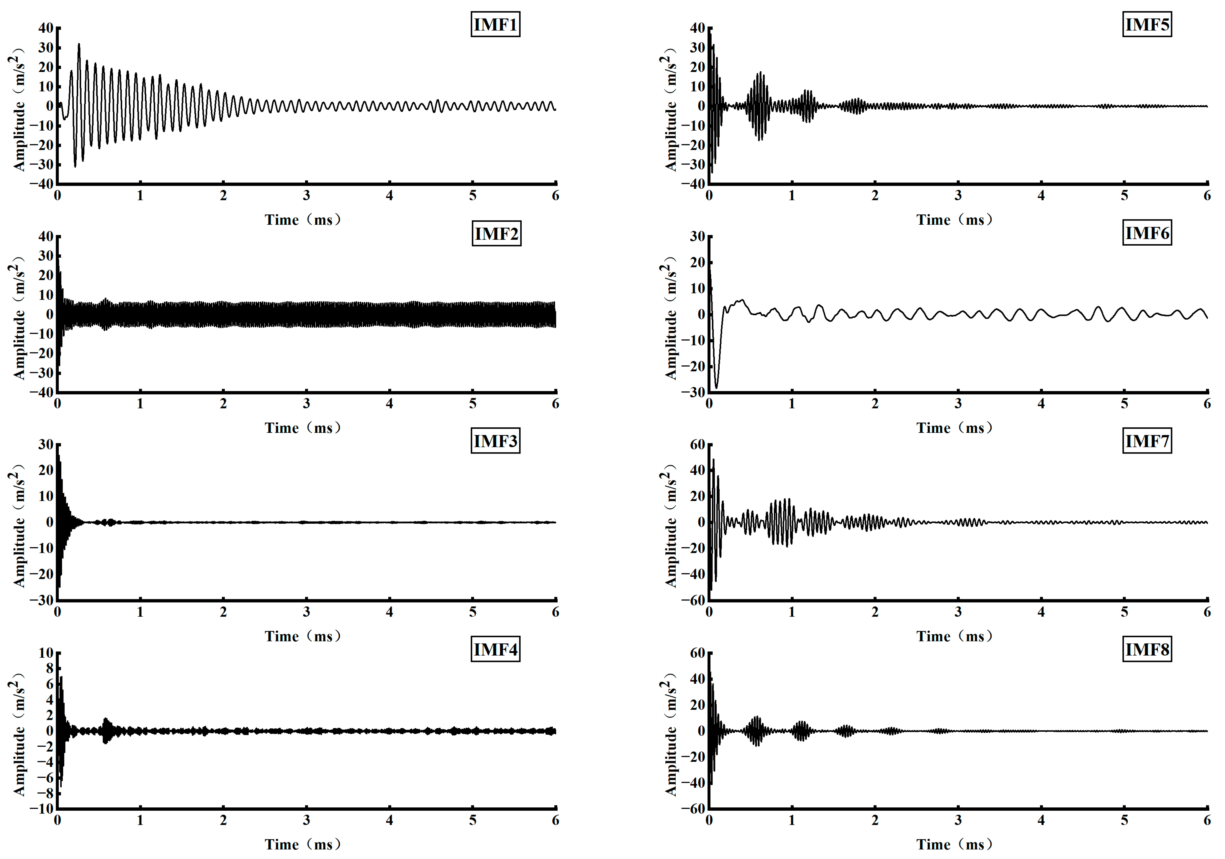
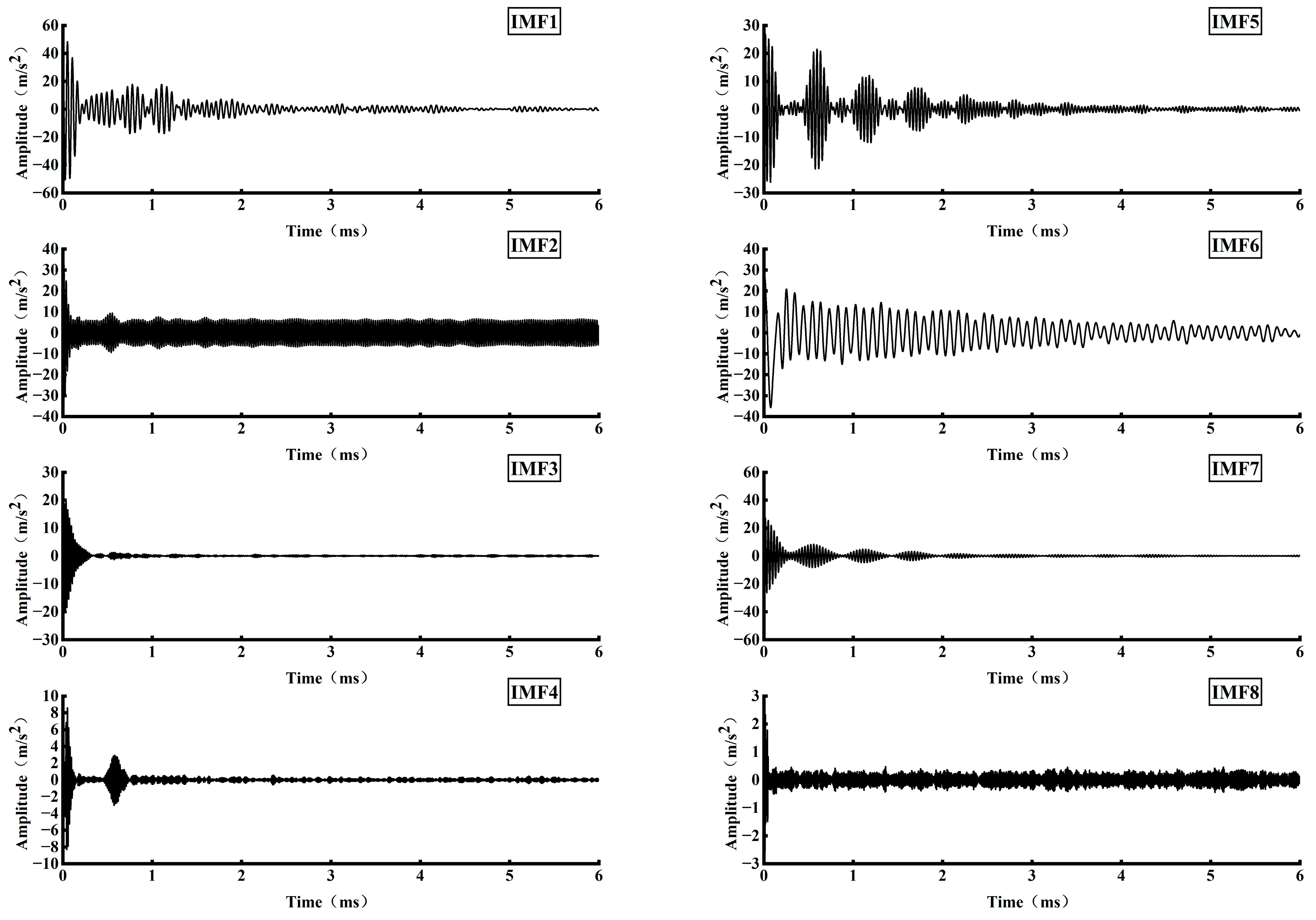
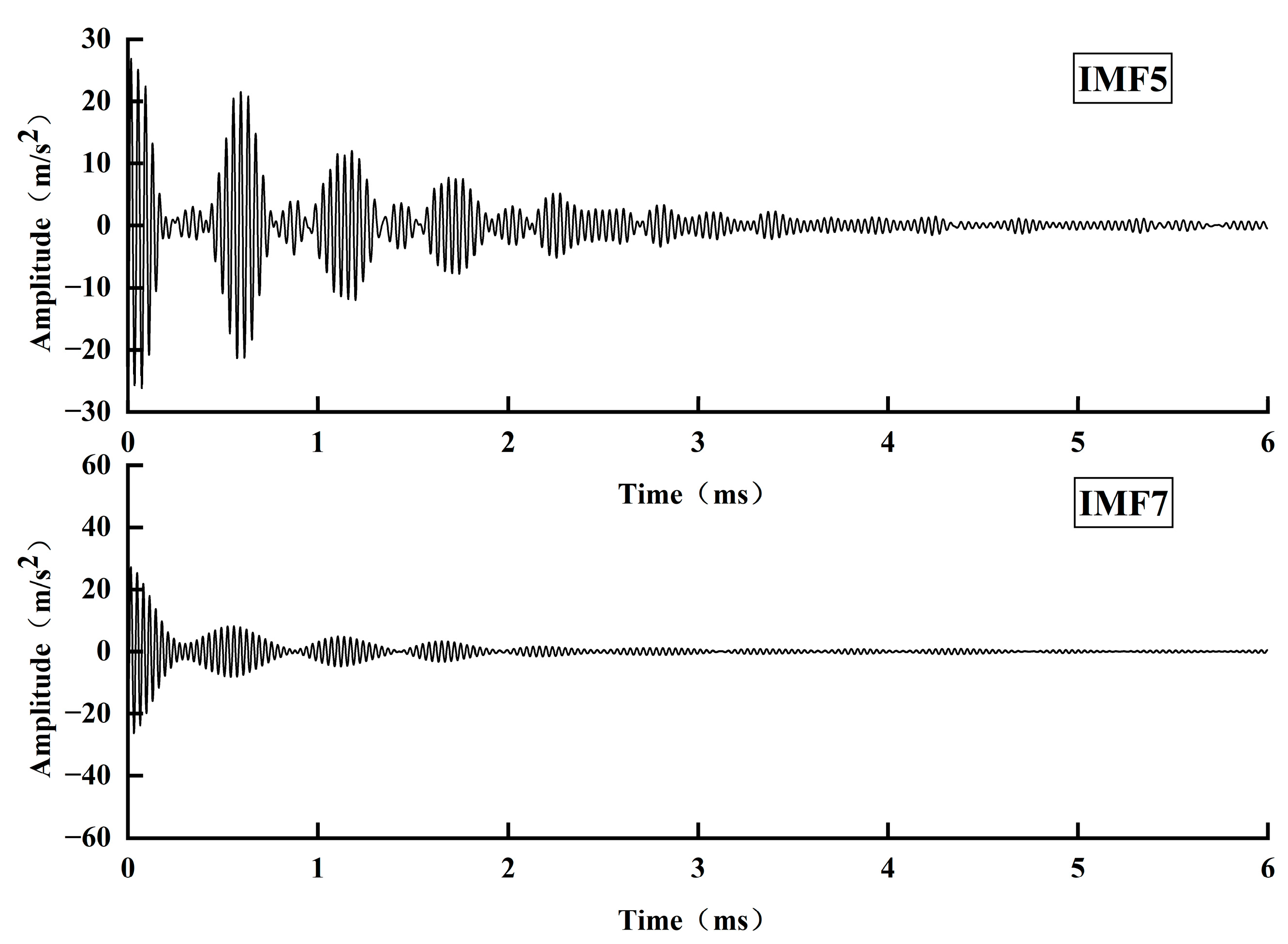
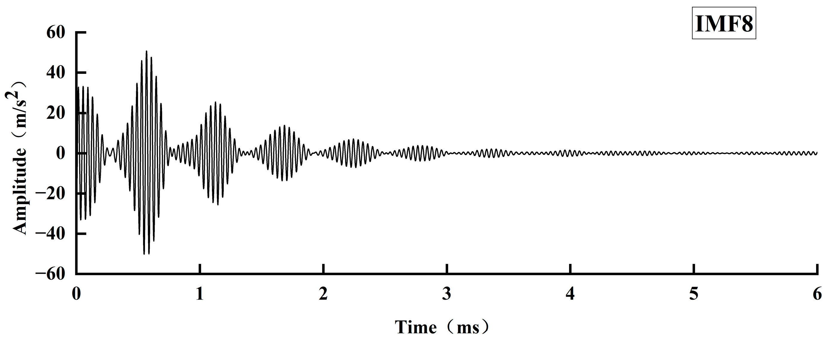
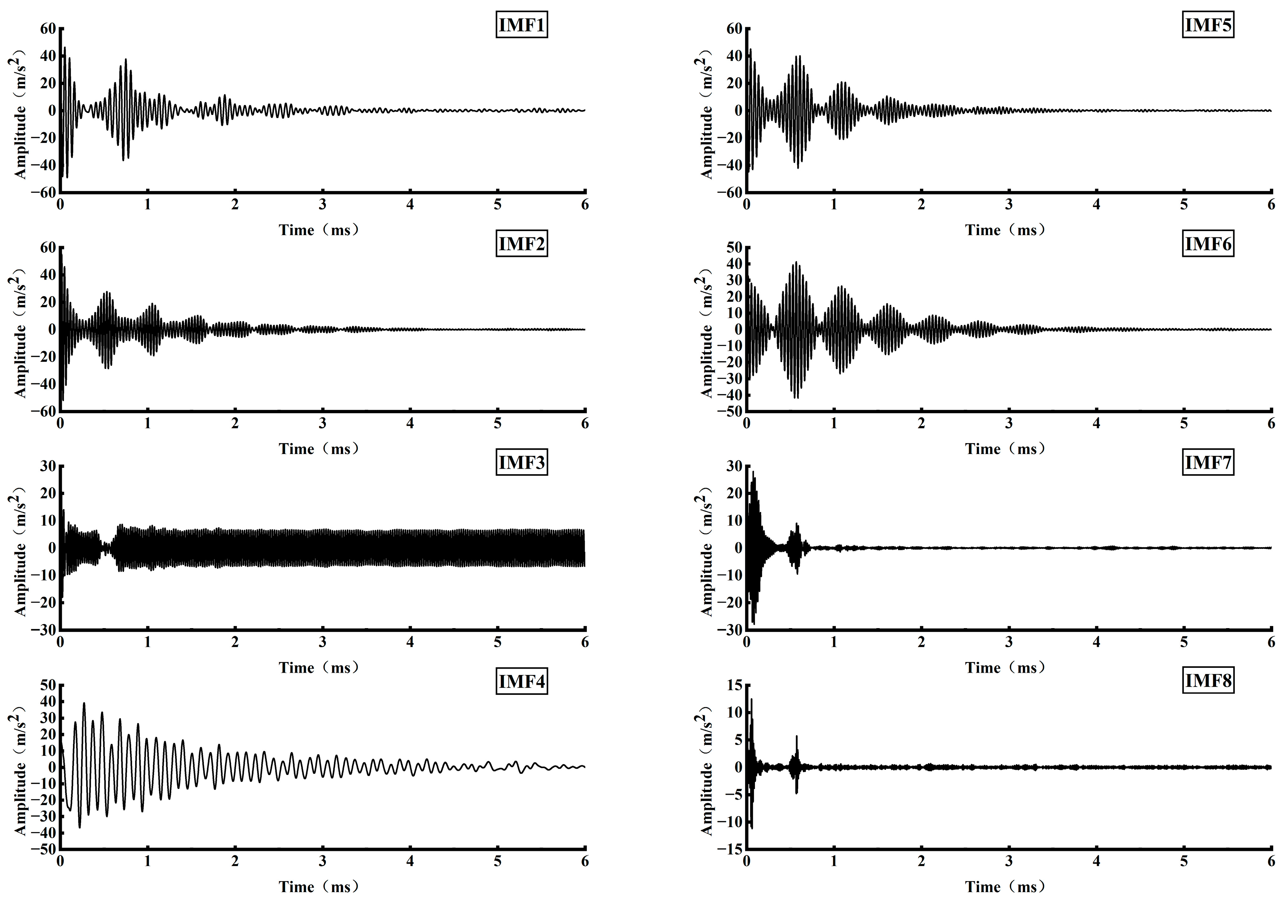
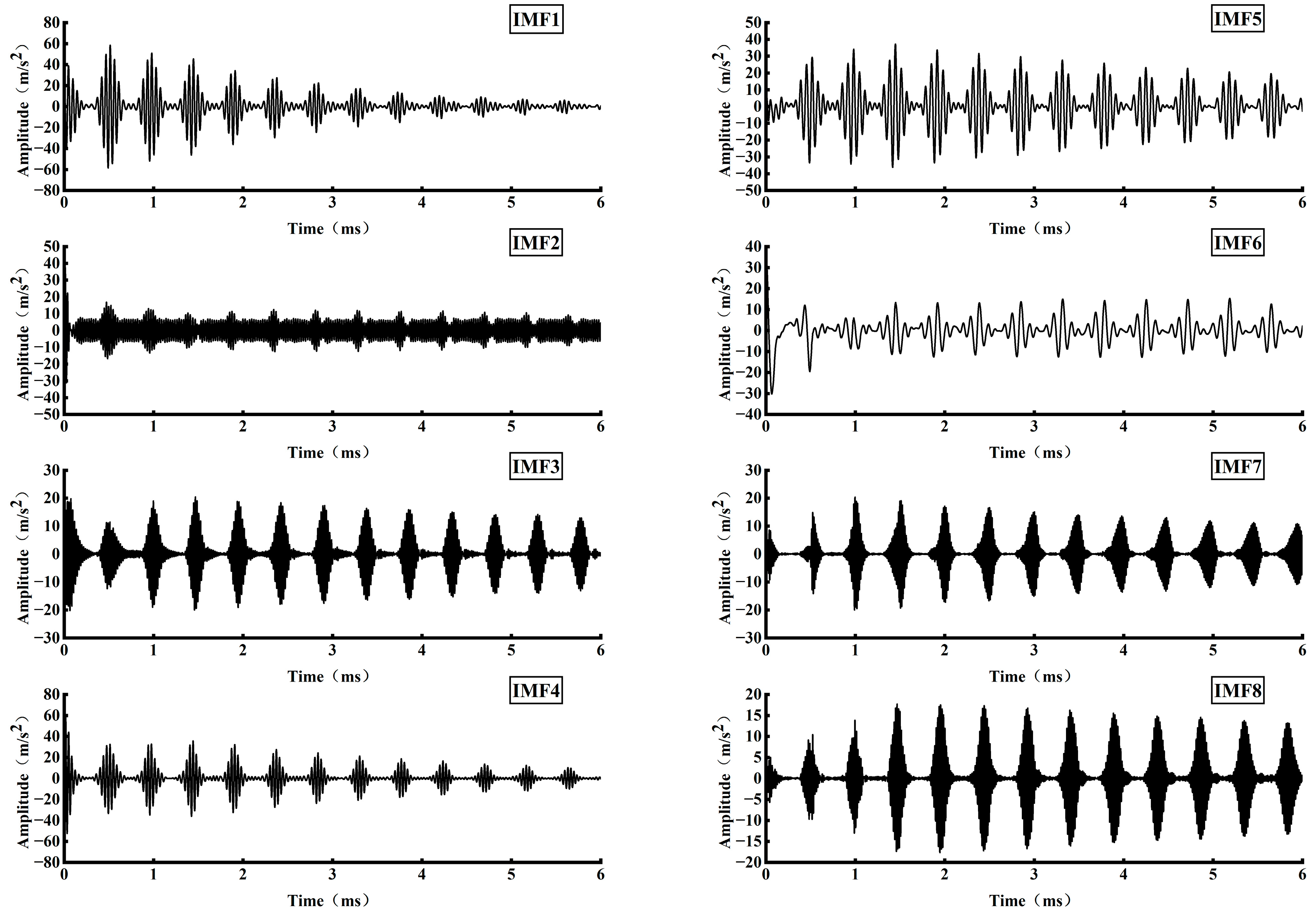
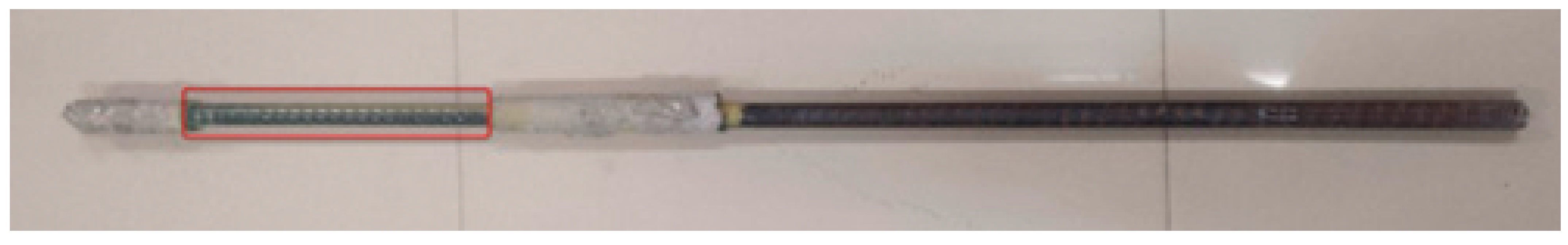
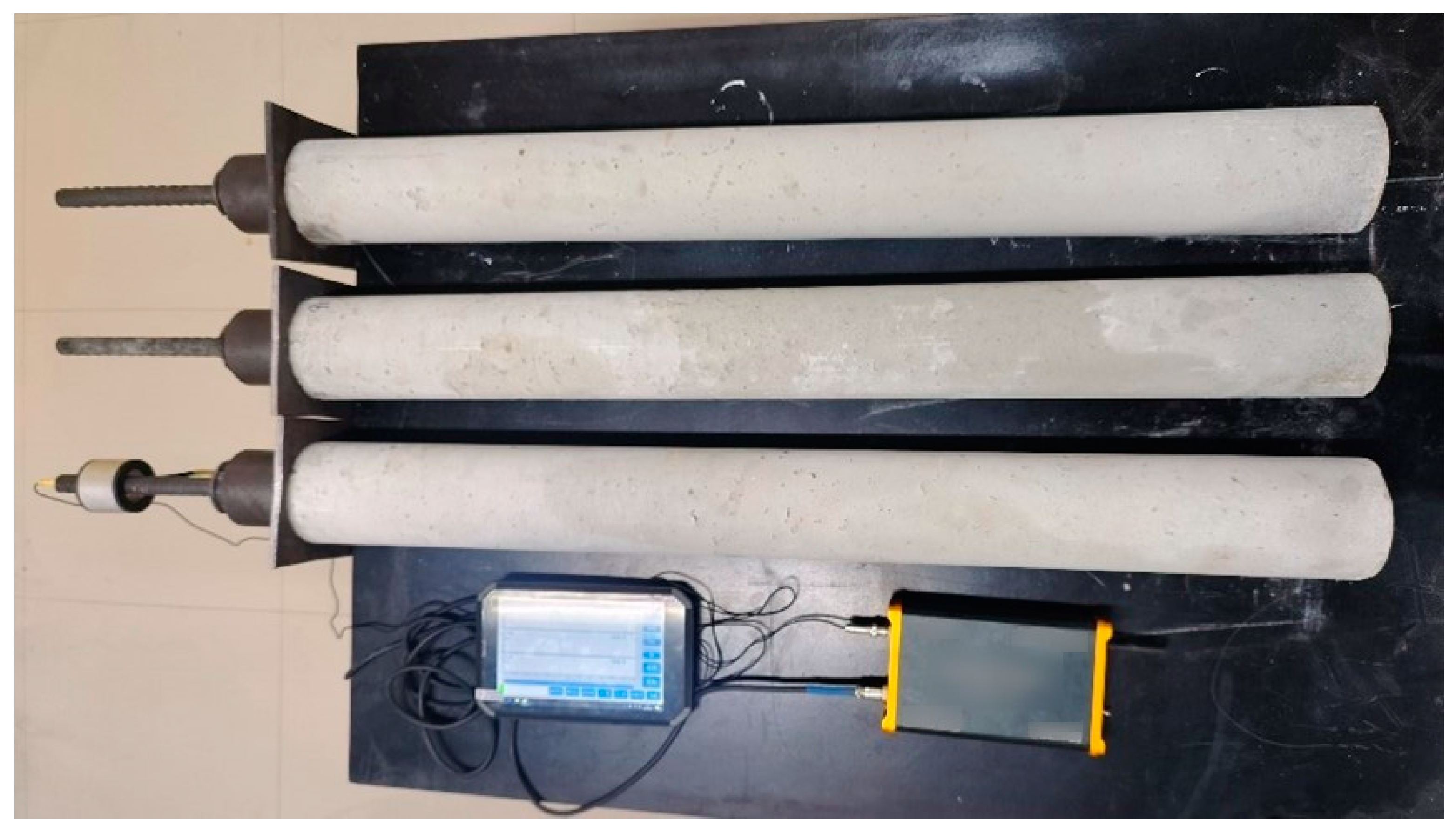
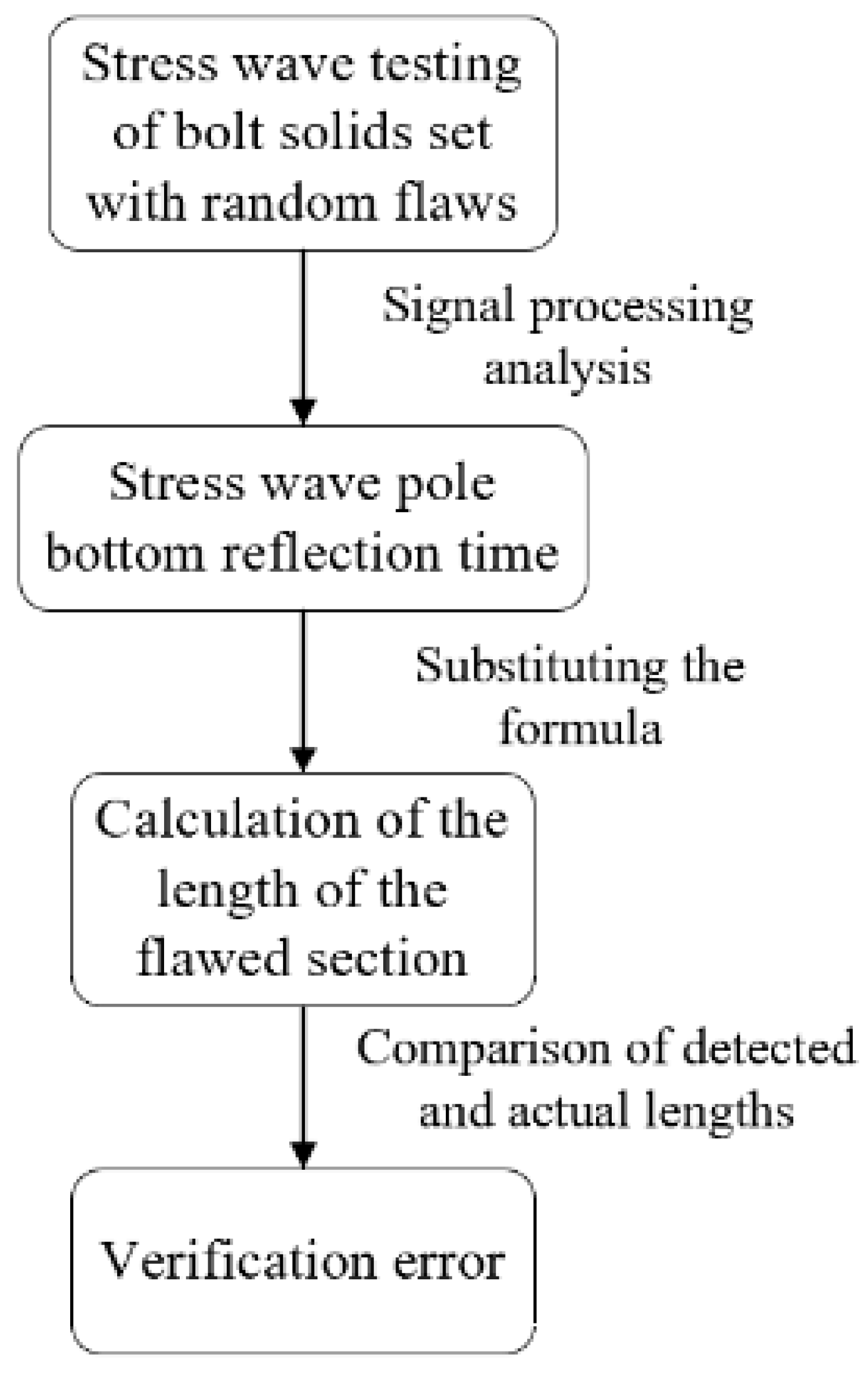
Based on the propagation law of stress waves in defective bolt solids, this paper proposed a stress wave anchorage defect detection method centered on analyzing the reflection at the bottom of the stress wave rod and the reflection phenomenon at the bottom of the bolt solid with different defect lengths. This was accomplished by building an experimental system of nondestructive testing of anchorage defects in a stress wave, and employing the VMD signal decomposition method. VMD is a powerful signal processing technique that decomposes a signal into a finite number of modes, each with a specific frequency range and amplitude. The key research findings are the following:

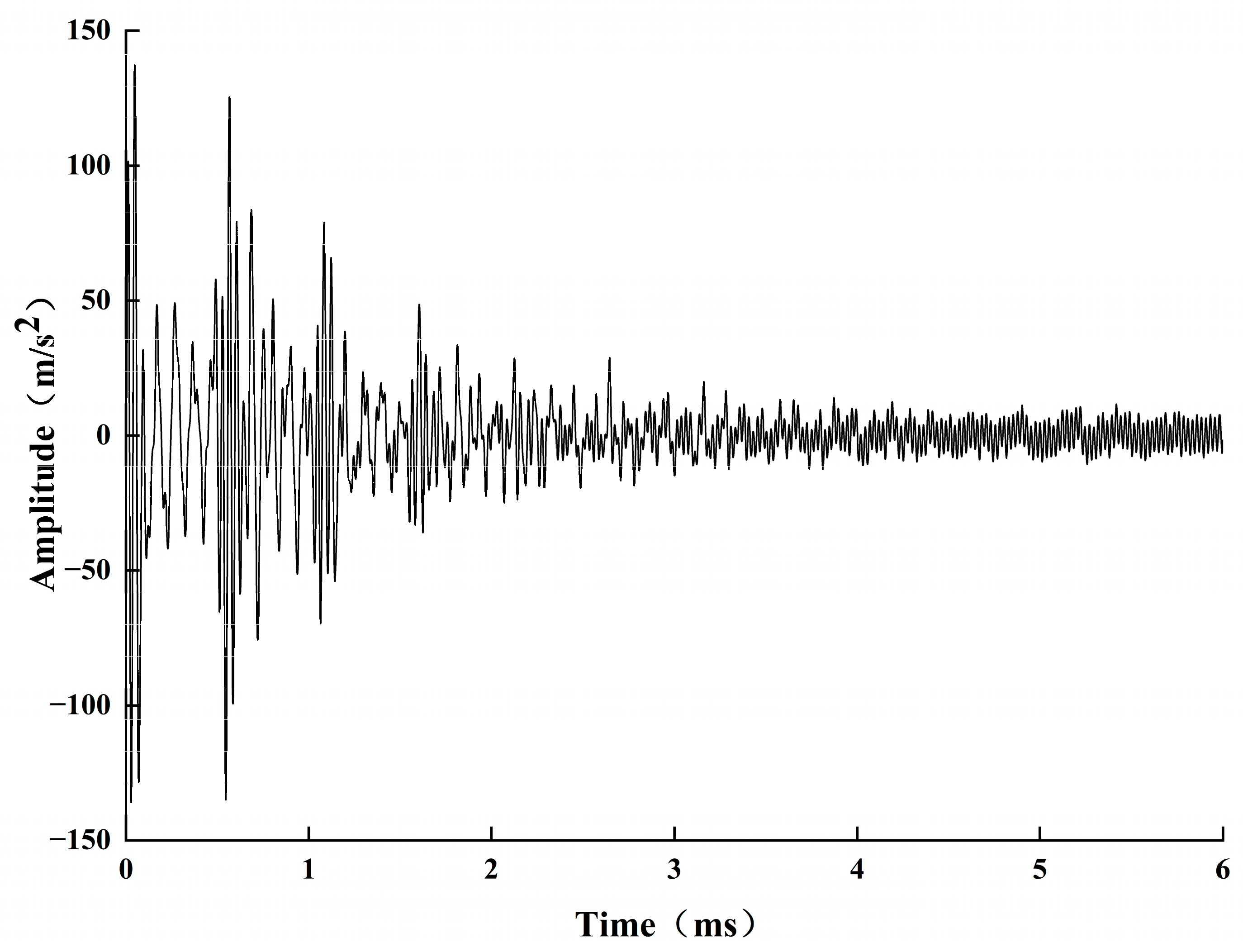
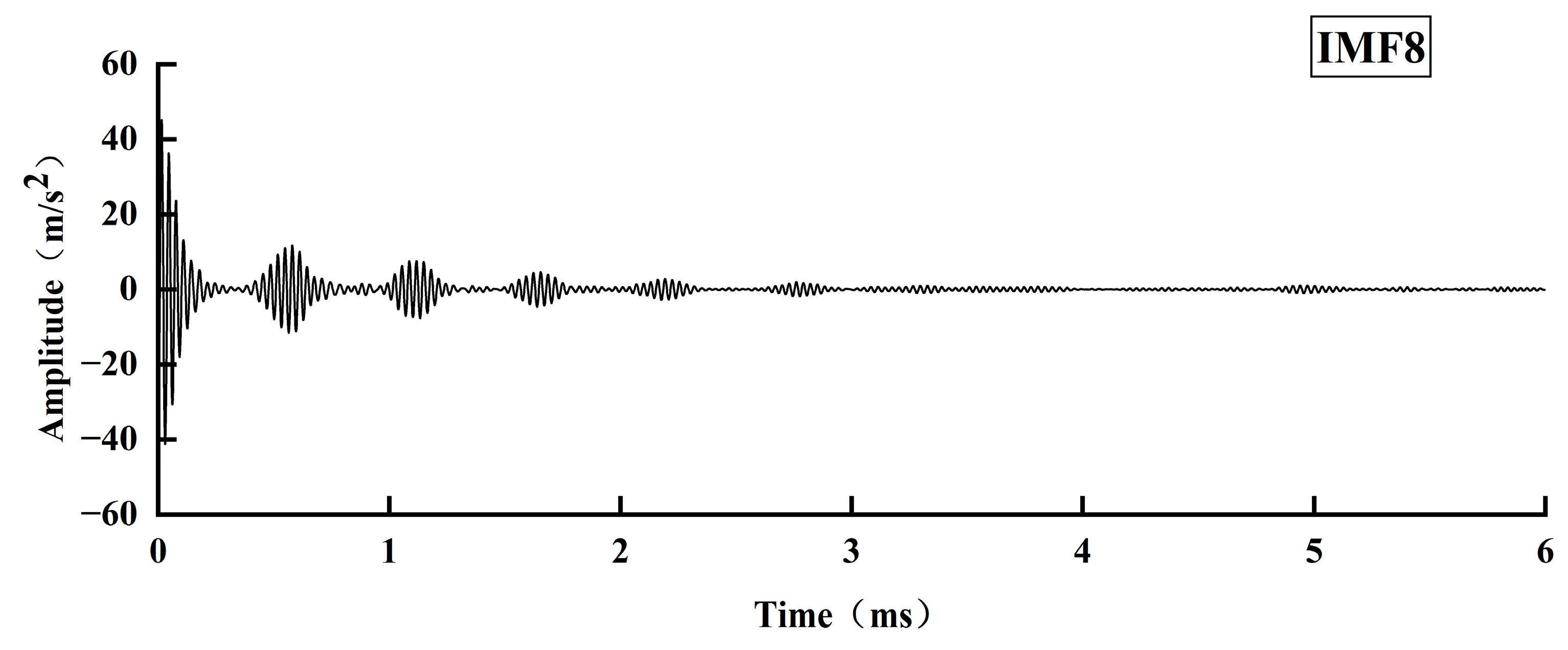
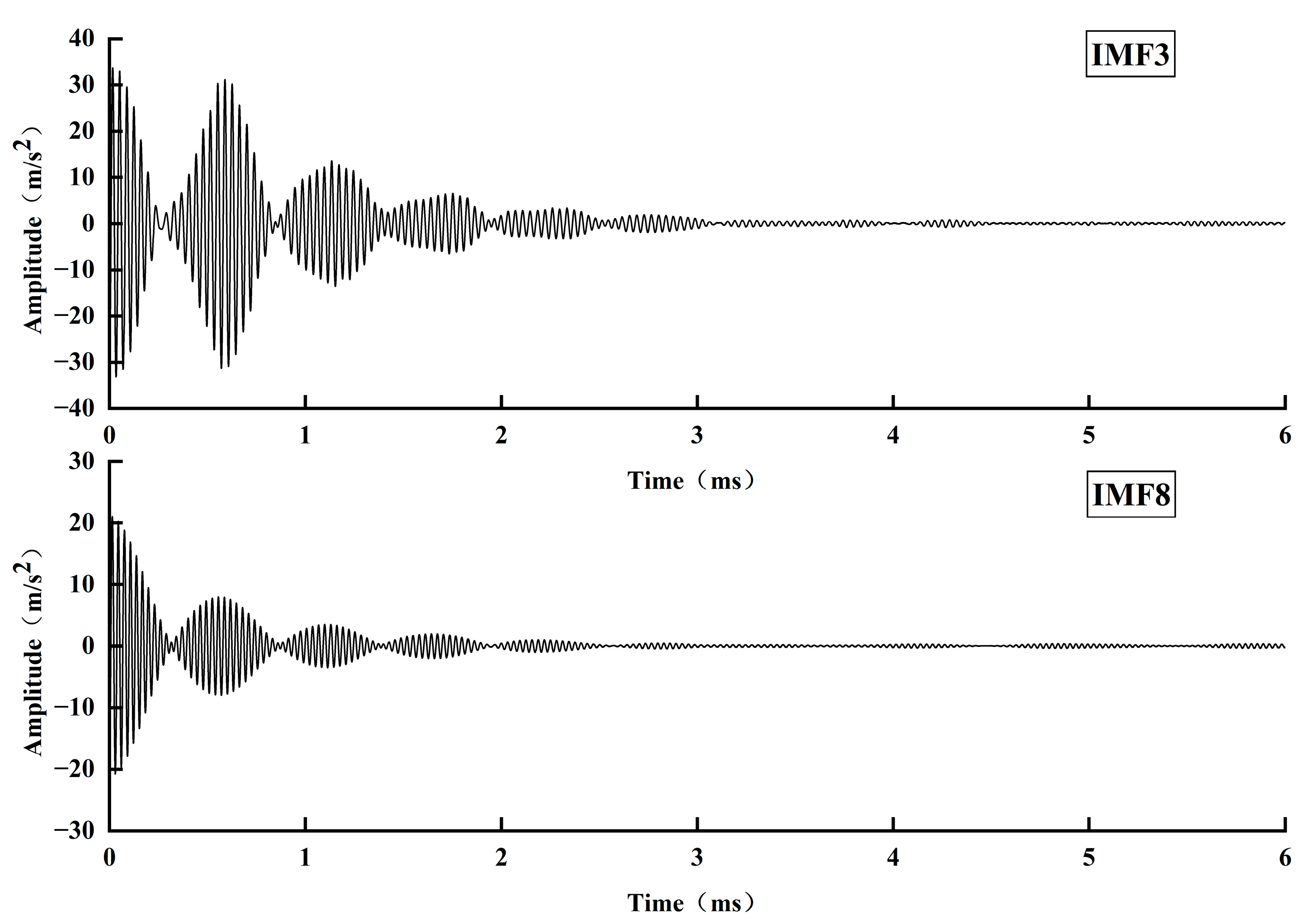
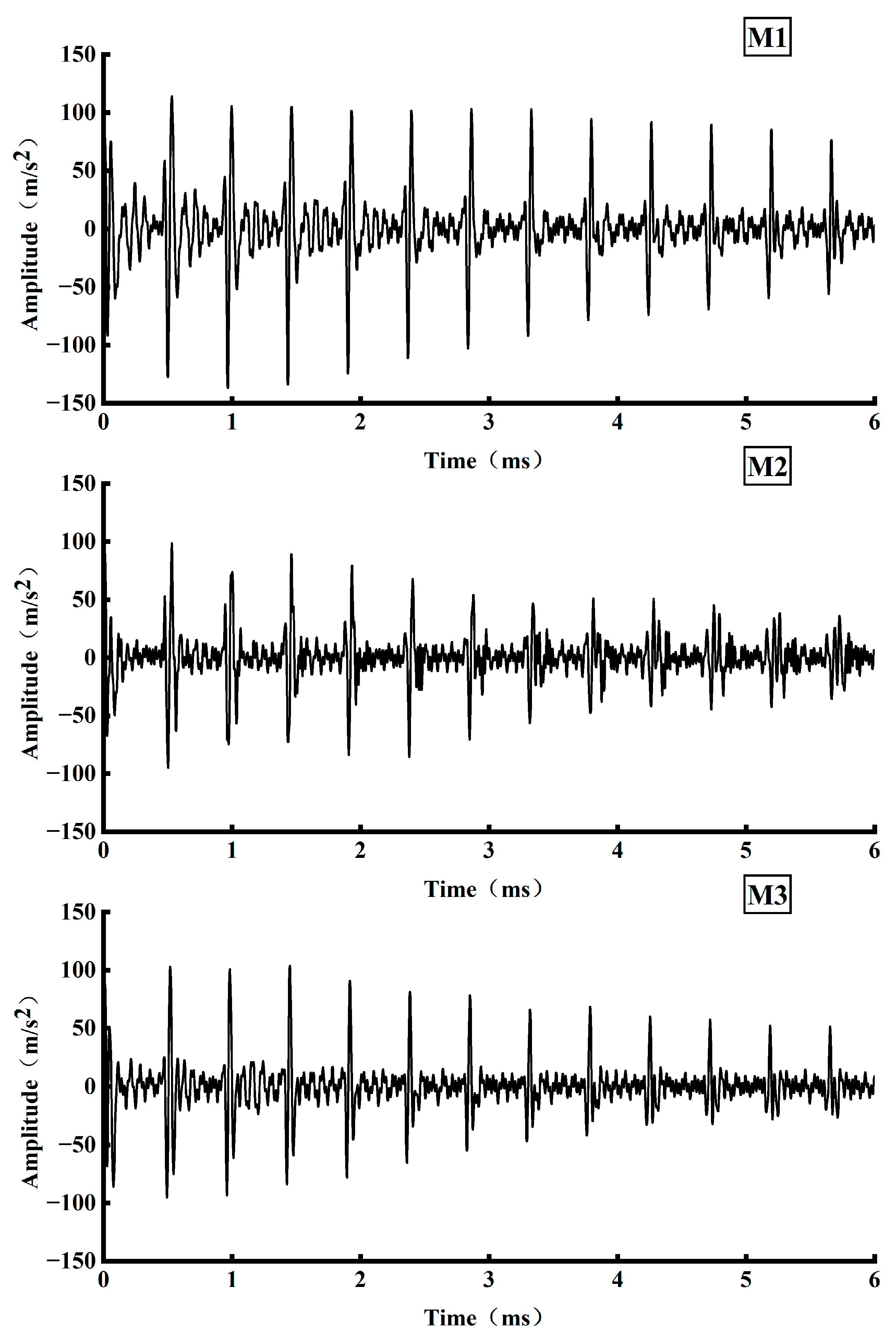
VMD decomposed the stress wave signals of specimens with different anchorage flaw lengths, and the characteristic modal signals obtained were analyzed in depth, from which the reflection time of the bottom of the rod of each specimen was determined. The analysis results show that the rod bottom reflection time is gradually shortened with the increase in the anchorage flaw length.

The rod bottom reflection time of specimens in different anchorage states was analyzed, and the propagation velocities of the excitation reflected stress wave in the free rod, anchorage section, and anchorage flaw section were 5150 m/s, 4198 m/s, and 5150 m/s, respectively. By taking the rod bottom reflection time as the key parameter for calculating the length of the anchorage flaws, the formula of the length of the anchorage flaws was proposed; it can provide a reference for the detection of the quality of the anchorage.

The calculation method of anchorage flaw length was used to verify the anchorage quality of several unknown flaws in the bolt solids. The results show that the proposed method can effectively detect anchorage flaws, with an average difference of 2.7 mm and an average error of 2.65%. This practical application of the method confirms its potential to be a valuable tool in the field of nondestructive testing.

References

1. Feng, C.; Liu, S.; Jia, H.; Fu, M.; He, D. Strengthening Device for Improving Shear Performance of Anchor Cable in Rock Support. Materials 2024, 17, 197. [Google Scholar] [CrossRef]
2. Shan, R.L.; Peng, Y.; Kong, X.S.; Xiao, Y.H.; Yuan, H.H.; Huang, B.; Zheng, Y. Research progress of coal roadway support technology at home and abroad. Chin. J. Rock Mech. Eng. 2019, 38, 2377–2403. [Google Scholar] [CrossRef]
3. Kang, H. Seventy years development and prospects of strata control technologies for coal mine roadways in China. Chin. J. Rock Mech. Eng. 2021, 40, 1–30. [Google Scholar] [CrossRef]
4. Seo, D.; Kim, J.; Park, S. An experimental study on defect detection of anchor bolts using non-destructive testing techniques. Materials 2023, 16, 4861. [Google Scholar] [CrossRef]
5. Hao, Y.; Wu, Y.; Ranjith, P.G.; Zhang, K.; Zhang, H.; Chen, Y.; Li, M.; Li, P. New insights on ground control in intelligent mining with Internet of Things. Comput. Commun. 2020, 150, 788–798. [Google Scholar] [CrossRef]
6. Zhang, X.; Wang, Z. Development and application of nondestructive testing methods for concrete. Nondestruct. Test. 2017, 39, 1–5. [Google Scholar] [CrossRef]
7. Dwivedi, S.K.; Vishwakarma, M.; Soni, A. Advances and researches on non destructive testing: A review. Mater. Today Proc. 2018, 5, 3690–3698. [Google Scholar] [CrossRef]
8. Gupta, M.; Khan, M.A.; Butola, R.; Singari, R.M. Advances in applications of Non-Destructive Testing (NDT): A review. Adv. Mater. Process. Technol. 2022, 8, 2286–2307. [Google Scholar] [CrossRef]
9. Vrkljan, I.; Szavits-Nossan, B.; Kovacevic, M.S. Nondestructive Procedure For Testing Grouting Quality of Rockbolt Anchors. Paper presented at the 9th ISRM Congress, Paris, France, 25–29 August 1999. [Google Scholar]
10. Teng, Y.; Hao, Y.Y.; Xue, X. Experimental research on grouting anchor Bar quality using nondestructive testing technology. Coal Eng. 2019, 51, 123–128. [Google Scholar]
11. Liu, L.L.; Zhu, J.; Zhang, S.H.; Sun, P.H. Non-destructive detection of anchor defects using ultrasonic guided wave and ICEEMDAN method. Earth Sci. 2022, 66, 1–17. [Google Scholar]
12. Naiyuan, Z. Study on Identification of Rockbolt Anchorage Defects Based on Ultrasonic Testing Method. Master’s Thesis, Northeastern University, Liaoning, China, 2021. [Google Scholar] [CrossRef]
13. Wang, Z.-Y.; Dou, L.-M.; Wang, G.-F.; Feng, L.-F.; Kang, K.; Bai, J.-Z.; Wang, S.-C. Resisting impact mechanical analysis of an anchored roadway supporting structure under P-wave loading and its application in rock burst prevention. Arab. J. Geosci. 2018, 11, 81. [Google Scholar] [CrossRef]
14. Fan, K.S.; Shen, B.H.; Liu, S.W.; Jiao, J.K. Numerical test and application of propagation characteristics of stress wave on roadway roof anchored body. J. Min. Saf. Eng. 2018, 28, 245–253. [Google Scholar] [CrossRef]
15. Li, J.C.; Fan, L.F.; Li, Z.L. Progress of methods for wave propagation across rock masses. Chin. J. Appl. Mech. 2022, 39, 845–858. [Google Scholar]
16. Sun, B.; Xie, J.-H.; Zeng, S. Synchronicity of Stress Wave Propagation in Bolt Body and Anchorage Medium. J. Eng. Technol. Sci. 2017, 49, 247–260. [Google Scholar] [CrossRef]
17. Fan, K. Experimental study on waveguide features of resin anchoring mass. Coal Sci. Technol. 2016, 11, 62–67. [Google Scholar] [CrossRef]
18. Niu, L.; Zhu, W.; Qin, C.; Zhang, N. The quality evaluation of the grout in rock bolts based on the stress wave propagation. IOP Conf. Series Earth Environ. Sci. 2021, 861, 042066. [Google Scholar] [CrossRef]
19. Huang, N.E.; Shen, Z.; Long, S.R.; Wu, M.C.; Shih, H.H.; Zheng, Q.; Yen, N.-C.; Tung, C.C.; Liu, H.H. The empirical mode decomposition and the Hilbert spectrum for nonlinear and non-stationary time series analysis. Proceedings of the Royal Society of London. Ser. A Math. Phys. Eng. Sci. 1998, 454, 903–995. [Google Scholar] [CrossRef]
20. Wu, Z.; Huang, N.E. Ensemble empirical mode decomposition: A noise-assisted data analysis method. Adv. Adapt. Data Anal. 2009, 1, 1–41. [Google Scholar] [CrossRef]
21. Torres, M.E.; Colominas, M.A.; Schlotthauer, G.; Flandrin, P. A complete ensemble empirical mode decomposition with adaptive noise. in 2011 IEEE international conference on acoustics, speech and signal processing (ICASSP). In Proceedings of the 2011 IEEE International Conference on Acoustics, Speech and Signal Processing (ICASSP), Prague, Czech Republic, 22–27 May 2011. [Google Scholar] [CrossRef]
22. Dragomiretskiy, K.; Zosso, D. Variational mode decomposition. IEEE Trans. Signal Process. 2013, 62, 531–544. [Google Scholar] [CrossRef]
23. Xu, J.; Ren, Q. A novel method of bolt detection based on variational modal decomposition. arXiv 2017, arXiv:1711.04388. [Google Scholar] [CrossRef]
24. Luo, Y.; Yao, Y.; Huang, C.; Zhang, J. Deformation feature extraction and analysis based on improved variational mode decomposition. Geomat. Inf. Sci. Wuhan Univ. 2020, 45, 612–619. [Google Scholar] [CrossRef]
25. Li, C.; Zhang, Z.; Li, C.; Feng, R.; Gao, X.; Bai, J.; Nie, B. A novel method of computation for anchorage length based on the propagation characteristics of anchor excitation stress wave. Nondestruct. Test. Eval. 2024, 1–36. [Google Scholar] [CrossRef]
26. Liu, W.; Yuan, W.; Yan, Y.; Wang, X. Analysis of Acoustic Emission Characteristics an Damage Constitutive Model of Coal-Rock Combined Body Based on Particle Flow Code. Symmetry 2019, 11, 1040. [Google Scholar] [CrossRef]
27. Peng, C.; Du, X.; Li, Z.; Liu, W.; Huang, B. Experimental and simulation study on compressive failure of rock with pre-Y-shaped cracks. PLoS ONE 2024, 19, e0312344. [Google Scholar] [CrossRef] [PubMed]
Figure 1. Schematic of stress wave propagation without flawed bolt solid.
Symmetry 17 00221 g001
Figure 2. Schematic of stress wave propagation in flawed bolt solid.
Symmetry 17 00221 g002
Figure 3. Original signal map of flawed bolt solid.
Symmetry 17 00221 g003
Figure 4. VMD decomposition flowchart.
Symmetry 17 00221 g004
Figure 5. Schematic diagram of bolt solid specimens with different bolt flaw lengths.
Symmetry 17 00221 g005
Figure 6. (a) Specimen production; (b) completed specimens.
Symmetry 17 00221 g006
Figure 7. Wireless anchor quality tester.
Symmetry 17 00221 g007
Figure 8. Specimen MG1-1 detection signal decomposition results.
Symmetry 17 00221 g008
Figure 9. IMF8 modal functions.
Symmetry 17 00221 g009
Figure 10. Specimen MG2-1 detection signal decomposition results.
Symmetry 17 00221 g010
Figure 11. IMF3 and IMF8 modal components.
Symmetry 17 00221 g011
Figure 12. Specimen MG31 detection signal decomposition results.
Symmetry 17 00221 g012
Figure 13. IMF5 and IMF7 modal components.
Symmetry 17 00221 g013
Figure 14. IMF5 quadratic decomposition results.
Symmetry 17 00221 g014
Figure 15. Specimen MG41 detection signal decomposition results.
Symmetry 17 00221 g015
Figure 16. IMF8 components.
Symmetry 17 00221 g016
Figure 17. Specimen MG51 detection signal decomposition results.
Symmetry 17 00221 g017
Figure 18. IMF2, IMF5, and IMF6 modal components.
Symmetry 17 00221 g018
Figure 19. Specimen MG61 detection signal decomposition results.
Symmetry 17 00221 g019
Figure 20. Bolts containing anchorage flaws.
Symmetry 17 00221 g020
Figure 21. Bolts with anchoring agent attached.
Symmetry 17 00221 g021
Figure 22. Time domain diagrams of M1, M2, and M3 specimens.
Symmetry 17 00221 g022
Figure 23. Verification of experimental specimen signal acquisition.
Symmetry 17 00221 g023
Figure 24. Validation test flow chart.
Symmetry 17 00221 g024
Figure 25. Specimen anchorage length verification: (a) Verification of specimen crushing results; (b) measurement of bolt flaw lengths.
Symmetry 17 00221 g025