Estimation and Bayesian Prediction for New Version of Xgamma Distribution Under Progressive Type-II Censoring

Abstract

This article introduces a new continuous lifetime distribution within the Gamma family, called the induced Xgamma distribution, and explores its various statistical properties. The proposed distribution’s estimation and prediction are investigated using Bayesian and non-Bayesian approaches under progressively Type-II censored data. The maximum likelihood and maximum product spacing methods are applied for the non-Bayesian approach, and some of their performances are evaluated. In the Bayesian framework, the numerical approximation technique utilizing the Metropolis–Hastings algorithm within the Markov chain Monte Carlo is employed under different loss functions, including the squared error loss, general entropy, and LINEX loss. Interval estimation methods, such as asymptotic confidence intervals, log-normal asymptotic confidence intervals, and highest posterior density intervals, are also developed. A comprehensive numerical study using Monte Carlo simulations is conducted to evaluate the performance of the proposed point and interval estimation methods through progressive Type-II censored data. Furthermore, the applicability and effectiveness of the proposed distribution are demonstrated through three real-world datasets from the fields of medicine and engineering.

1. Introduction

The development of new probability distributions plays a crucial role in statistical modeling, particularly in reliability engineering, survival analysis, and actuarial science. In many real-world applications, existing distributions fail to adequately capture the complexity of observed data, leading to the need for more flexible and robust models (see [1,2,3,4,5,6,7,8,9,10,11,12]). One such challenge arises in studying lifetime data, where traditional distributions may not fully accommodate various hazard-rate behaviors. This motivates the derivation of new probability models that better describe real-world phenomena.

For the PCT-II approach, ref. [2] created an algorithm to simulate general PCT-II samples from uniform or other continuous distributions. Some procedures for the estimation of parameters from different lifetime distributions based on PCT-II were developed by many authors, which include [1,13,14,15,16,17,18,19,20,21,22,23,24,25,26,27,28,29]. Recently, ref. [28] looked at the A and D optimal censoring plans in the PCT-II scheme order statistics. Ref. [26] suggested a new test statistic based on spacings to see if the samples from the general PCT-II scheme are from an exponential distribution. Ref. [30] estimated a Burr distribution’s unknown parameters, reliability, and hazard functions under the PCT-II sample.

Ref. [31] showed that when a controlled stepwise sample of the second type was available, parametric (classical and Bayes) point estimation procedures could be used to determine reliability characteristics, such as the reliability function and the mean time to failure for the Xgamma distribution, based on all observations.

To demonstrate the PCT-II scheme analyzing methods, the examiner gives different but identical units to the life test. There are n units to be tested at the beginning of the experiment, and the test ends when the mth $(m<n)$ unit fails. Once one unit fails, the time $x_{\left(1\right)}$ is recorded and $R_1$ units are randomly selected from the remaining survival units $n-1$. Again, when the second unit fails, the time $x_{\left(2\right)}$ will be recorded, and $R_2$ units are then randomly withdrawn from the remaining $n-R_1-2$ survival units. This experiment stops at the mth failure, which is determined in advance, at time $x_m$, and $R_m=n-m-{\displaystyle \sum _{i=1}^{m-1}}{R}_i$. The likelihood function based on a PCT-II sample $\{x_{\left(i\right)},R_i\}$ is given by (see, [1]):

$$L\left(\theta \right)=C\underset{i=1}{{\displaystyle \prod }^m}f(x_{\left(i\right)};\theta ){\left[1-F(x_{\left(i\right)};\theta )\right]}^{R_i},$$

(1)

where C is defined as $C=n\left(n-1-R_1\right)\left(n-2-R_1-R_2\right)\cdots \left(n-{\sum }_{i=1}^{m-1}\left(R_i+1\right)\right),$ and $F(·)$ and $f(·)$ represent the cumulative distribution function (Cdf) and probability density function (Pdf), respectively. For the representation of the PCT-II scheme, Figure 1 illustrates the PCT-II scheme.

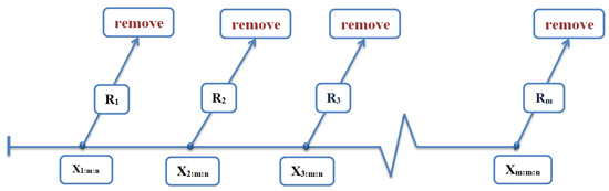
Figure 1. Visualization of PCT-II scheme.

This article introduces a new probability distribution using the concept of an induced distribution. Let X be a continuous random variable with Pdf $g\left(x\right)$, Cdf $G\left(x\right)$, and expectation $E\left(X\right)$. We define an induced Pdf $f\left(x\right)$ as:

$$f\left(x\right)={\displaystyle \frac{1-G\left(x\right)}{E\left(X\right)}},x>0.$$

It is well known that:

$$E\left(X\right)={\int }_0^{\infty }[1-G\left(x\right)]dx<\infty .$$

Thus, the induced Pdf $f\left(x\right)$ can be rewritten as:

$$f\left(x\right)={\displaystyle \frac{1-G\left(x\right)}{{\int }_0^{\infty }[1-G\left(x\right)]dx}},x>0.$$

(2)

The assumed $G\left(x\right)$ is the Xgamma distribution which was proposed by [16] with Pdf and Cdf, respectively, given by:

$$g(x;\theta )={\displaystyle \frac{{\theta }^2}{1+\theta }}\left(1+{\displaystyle \frac{\theta x^2}{2}}\right)e^{-\theta x};x,\theta >0,$$

(3)

and

$$G(x;\theta )=1-{\displaystyle \frac{1}{1+\theta }}\left(1+\theta +\theta x+{\displaystyle \frac{{\theta }^2{x}^2}{2}}\right)e^{-\theta x};x,\theta >0,$$

(4)

Many of the statistical characteristics of this distribution are easily studied, and it exhibits a strong relationship with its parent distribution, i.e., the Xgamma distribution. The Xgamma distribution is chosen for its flexibility in modeling lifetime data, combining gamma and exponential properties, and adapting well to progressive Type-II censoring (PCT-II), and it exhibits similar properties to the Lindley distribution. Using the approach described in Equation (2), where $E\left(X\right)$ is the mean of the random variable $X\sim \mathrm{Xgamma}\left(\theta \right)$, we derive the Pdf of the new distribution, which we term the induced Xgamma distribution (iXgamma). Hence, the Pdf of the iXgamma distribution is obtained by substituting $G(x;\theta )$ from Equation (4) into Equation (2). It is expressed as:

$$f(x;\theta )={\displaystyle \frac{\theta }{3+\theta }}\left(1+\theta +\theta x+{\displaystyle \frac{{\theta }^2{x}^2}{2}}\right)e^{-\theta x},x,\theta >0.$$

(5)

The Cdf of the iXgamma distribution can be derived by integrating Equation (5) concerning x. It is given by:

$$F(x;\theta )=1-\left[1+{\displaystyle \frac{\theta }{\theta +3}}\left(2x+{\displaystyle \frac{\theta x^2}{2}}\right)\right]e^{-\theta x},x,\theta >0.$$

(6)

Proof. 

We know,

$$\begin{array}{ccc}\hfill F(x,\theta )& =& {\int }_0^{x}f\left(t\right)dt\hfill \\ & =& {\int }_0^x{\displaystyle \frac{\theta }{3+\theta }}\left(1+\theta +\theta t+{\displaystyle \frac{{\theta }^2{t}^2}{2}}\right)e^{-\theta t}dt\hfill \\ & =& {\displaystyle \frac{\theta }{3+\theta }}{\int }_0^x\left(e^{-\theta t}dt+\theta e^{-\theta t}dt+\theta t{e}^{-\theta t}dt+{\displaystyle \frac{{\theta }^2{t}^2}{2}}{e}^{-\theta t}dt\right)\hfill \\ & =& {\displaystyle \frac{\theta }{3+\theta }}{\left[{\displaystyle \frac{-e^{-\theta t}}{\theta }}-{\displaystyle \frac{\theta e^{-\theta t}}{\theta }}-{\displaystyle \frac{e^{-\theta t}(\theta t+1)}{\theta }}-{\displaystyle \frac{e^{-\theta t}\left({\theta }^2{t}^2+2\theta t+2\right)}{2\theta }}\right]}_0^x\hfill \\ & =& 1-\left[1+{\displaystyle \frac{\theta }{\theta +3}}\left(2x+{\displaystyle \frac{\theta x^2}{2}}\right)\right]e^{-\theta x}.\hfill \end{array}$$

□

The newly proposed iXgamma distribution can also be expressed as a form of the following mixture:

$$f(x;\theta )=p_1{g}_1\left(x\right)+p_2{g}_2\left(x\right)+p_3{g}_3\left(x\right)$$

where

$$g_1\left(x\right)=\mathrm{Exp}\left(\theta \right),g_2\left(x\right)=\mathrm{Gamma}(2,\theta )\mathrm{and}{g}_3\left(x\right)=\mathrm{Gamma}(3,\theta ),$$

and

$$p_1={\displaystyle \frac{1+\theta }{3+\theta }},p_2={\displaystyle \frac{1}{3+\theta }},p_3={\displaystyle \frac{1}{3+\theta }}.$$

Proof. 

$$\begin{array}{ccc}\hfill f(x;\theta )& =& p_1{g}_1\left(x\right)+p_2{g}_2\left(x\right)+p_3{g}_3\left(x\right)\hfill \\ & =& {\displaystyle \frac{1+\theta }{3+\theta }}\mathrm{Exp}\left(\theta \right)+{\displaystyle \frac{1}{3+\theta }}\mathrm{Gamma}(2,\theta )+{\displaystyle \frac{1}{3+\theta }}\mathrm{Gamma}(3,\theta )\hfill \\ & =& {\displaystyle \frac{1+\theta }{3+\theta }}\theta e^{-\theta x}+{\displaystyle \frac{1}{3+\theta }}{\displaystyle \frac{{\theta }^2}{\Gamma 2}}{x}^{2-1}{e}^{-\theta x}+{\displaystyle \frac{1}{3+\theta }}{\displaystyle \frac{{\theta }^3}{\Gamma 3}}{x}^{3-1}{e}^{-\theta x}\hfill \\ & =& {\displaystyle \frac{\theta }{\theta +3}}\left[(1+\theta )e^{\theta x}+\theta x{e}^{-\theta x}+{\displaystyle \frac{{\theta }^2{x}^2}{2}}{e}^{\theta x}\right]\hfill \\ & =& {\displaystyle \frac{\theta }{3+\theta }}\left(1+\theta +\theta x+{\displaystyle \frac{{\theta }^2{x}^2}{2}}\right)e^{-\theta x}.\hfill \end{array}$$

□

The Pdf and Cdf plots for the iXgamma distribution with different values of $\theta$ are shown in Figure 2. These plots exhibit characteristics similar to those of the exponential distribution.

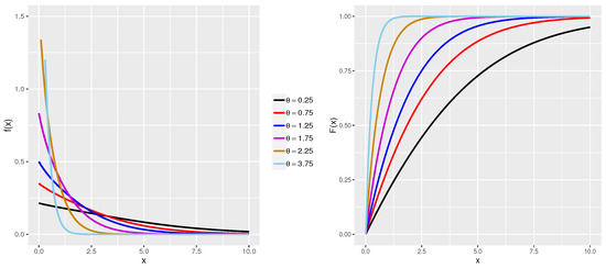
Figure 2. The graph of Pdf and Cdf of iXgamma for different values of $\theta$.

The novelty of our research is defined in three key aspects. First, we derived a new distribution based on the concept of induced distributions, as given in Equation (2), utilizing $G\left(x\right)\sim \mathrm{Xgamma}\left(\theta \right)$, leading to the proposed iXgamma distribution. Second, our proposed distribution is not merely an extension of the Xgamma distribution but rather a hybrid approach that integrates two fundamental distributions in mathematical statistics and reliability analysis—the Gamma and exponential distributions.

The limitations and challenges of this work are primarily related to the complexity of parameter estimation, computational intensity, limited sample sizes, model power, prediction, and inference difficulties. Advanced statistical methods and thorough evaluation of the data details and the censoring scheme are frequently needed to address these problems. Due to their costly numerical evaluations and complicated outcomes, new extended-gamma (iXgamma) lifetime models receive little attention from researchers. To our knowledge, no attempt has been made to estimate the iXgamma parameters based on the PCT-II scheme since the iXgamma distribution was presented in the literature, except for the work of [32], who used a complete sample to study Bayesian inferences based on non-informative priors.

The rest of the article is organized as follows: Section 2 introduces properties of the proposed iXgamma distribution. We discussed the maximum likelihood estimation and maximum product spacing estimation in Section 3. In Section 4, we present the Bayesian inferences and in Section 5, the confidence intervals estimations are presented. Simulation investigations and discussion are highlighted in Section 6. Three real datasets are analyzed in Section 7. In Section 8, point prediction is addressed using the maximum likelihood predictor and the Bayesian predictor. Finally, various observations are made in Section 9.

2. Properties of the Proposed iXgamma Distribution

In this section, various statistical and mathematical properties of the proposed distribution are explored, including reliability analysis, the distribution of order statistics, and the reliability of the stress strength and moments.

2.1. Reliability and Hazard Rate Function

The reliability $R(·)$ and hazard rate function for the iXgamma distribution are given, respectively, by:

$$\begin{array}{c}\hfill R\left(x\right)=P(X>x)=\left[1+{\displaystyle \frac{\theta }{\theta +3}}(2x+{\displaystyle \frac{\theta x^2}{2}})\right]e^{-\theta x}.\end{array}$$

$$\begin{array}{c}\hfill r\left(x\right)={\displaystyle \frac{f\left(x\right)}{R\left(x\right)}}={\displaystyle \frac{\theta \left(1+\theta +\theta x+\frac{{\theta }^2{x}^2}{2}\right)}{\left(3+\theta +2\theta x+\frac{{\theta }^2{x}^2}{2}\right)}}.\end{array}$$

It should be noted that ${\displaystyle \frac{\theta (1+\theta )}{3+\theta }}\le r\left(x\right)<\theta .$ The plot of the reliability and hazard rate functions of the iXgamma for different $\theta$ are given in Figure 3.

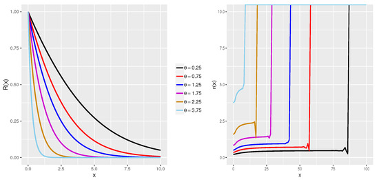
Figure 3. The reliability and hazard rate functions plot of iXgamma for different values of $\theta$.

The mean residual life (MRL) function of iXgamma is given by

$$\begin{array}{c}\hfill MRL\left(x\right)=P(X-x|X>x)={\displaystyle \frac{6+\theta +3\theta x+0.5{\theta }^2{x}^2}{\theta \left(3+\theta +2\theta x+0.5{\theta }^2{x}^2\right)}},\end{array}$$

and ${\displaystyle \frac{1}{\theta }}<MRL\left(x\right)\le {\displaystyle \frac{6+\theta }{\theta (3+\theta )}}$. Note that

$$MRL\left(0\right)={\displaystyle \frac{\theta +6}{\theta (\theta +3)}}={\mu }_1^{\prime }=E\left(X\right).$$

2.2. Quantile Function

The quantile function is defined as the inverse of the Cdf, $F\left(x\right)$. It satisfies the relationship:

$$F(x;\theta )=u\Rightarrow x=F^{-1}(u;\theta ),$$

where u follows a standard uniform distribution. For the iXgamma distribution, the percentiles cannot be expressed in a closed-form analytical solution due to the complexity of its Cdf. Thus, numerical methods are typically used to compute the quantile function.

2.3. Moments

The rth order moment for the iXgamma distribution is given by

$$\begin{array}{c}\hfill {\mu }_r^{\prime }={\displaystyle \frac{r!}{{\theta }^r(3+\theta )}}\left[(1+\theta )+(r+1)\left({\displaystyle \frac{r+4}{2}}\right)\right].\end{array}$$

Proof. 

We know,

$$\begin{array}{ccc}\hfill {\mu }_r^{\prime }& =& E\left(X^r\right)\hfill \\ & =& {\int }_0^{\infty }{x}^r{\displaystyle \frac{\theta }{3+\theta }}\left(1+\theta +\theta x+{\displaystyle \frac{{\theta }^2{x}^2}{2}}\right)e^{-\theta x}dx\hfill \\ & =& {\displaystyle \frac{\theta }{3+\theta }}{\int }_0^{\infty }{x}^r\left(1+\theta +\theta x+{\displaystyle \frac{{\theta }^2{x}^2}{2}}\right)e^{-\theta x}dx\hfill \\ & =& {\displaystyle \frac{\theta }{3+\theta }}{\int }_0^{\infty }\left[x^r{e}^{-\theta x}dx+\theta x^r{e}^{-\theta x}dx+\theta x^{r+1}{e}^{-\theta x}dx+{\displaystyle \frac{{\theta }^2}{2}}{x}^{r+2}{e}^{-\theta x}dx\right]\hfill \\ & =& {\displaystyle \frac{\theta }{3+\theta }}\left[{\int }_0^{\infty }{x}^r{e}^{-\theta x}dx+\theta {\int }_0^{\infty }{x}^r{e}^{-\theta x}dx+\theta {\int }_0^{\infty }{x}^{r+1}{e}^{-\theta x}dx+{\displaystyle \frac{{\theta }^2}{2}}{\int }_0^{\infty }{x}^{r+2}{e}^{-\theta x}dx\right]\hfill \\ & =& {\displaystyle \frac{\theta }{3+\theta }}\left[{\int }_0^{\infty }{x}^{(r+1)-1}{e}^{-\theta x}dx+\theta {\int }_0^{\infty }{x}^{(r+1)-1}{e}^{-\theta x}dx+\theta {\int }_0^{\infty }{x}^{(r+2)-1}{e}^{-\theta x}dx+{\displaystyle \frac{{\theta }^2}{2}}{\int }_0^{\infty }{x}^{(r+3)-1}{e}^{-\theta x}dx\right]\hfill \\ & =& {\displaystyle \frac{\theta }{3+\theta }}\left[{\displaystyle \frac{(1+\theta )\Gamma (r+1)}{{\theta }^{r+1}}}+{\displaystyle \frac{\theta \Gamma (r+2)}{{\theta }^{r+2}}}+{\displaystyle \frac{{\theta }^2\Gamma (r+3)}{2{\theta }^{r+3}}}\right]\hfill \\ & =& {\displaystyle \frac{r!}{{\theta }^r(3+\theta )}}\left[1+\theta +r+1+{\displaystyle \frac{(r+2)(r+1)}{2}}\right]\hfill \\ & =& {\displaystyle \frac{r!}{{\theta }^r(3+\theta )}}\left[(1+\theta )+(r+1)\left({\displaystyle \frac{r+4}{2}}\right)\right].\hfill \end{array}$$

□

In particular,

$${\mu }_1^{\prime }={\displaystyle \frac{\theta +6}{\theta (\theta +3)}}=E\left(X\right)=\mu ,$$

$${\mu }_2^{\prime }={\displaystyle \frac{2(\theta +10)}{{\theta }^2(\theta +3)}}$$

$${\mu }_2={\displaystyle \frac{{\theta }^2+14\theta +24}{{\theta }^2{(\theta +3)}^2}}$$

Using the recursive relation of raw and central moments, we can derive the skewness ($\sqrt{{\beta }_1}$), kurtosis (${\beta }_2$), and coefficient of variation ($CV$) as follows:

$$\begin{array}{c}\hfill \sqrt{{\beta }_1}={\displaystyle \frac{{\mu }_3^2}{{\mu }_2^3}},{\beta }_2={\displaystyle \frac{{\mu }_4}{{\mu }_2^2}},CV={\displaystyle \frac{{\mu }_2}{{\mu }_1^{\prime }}}.\end{array}$$

In Table 1, the values of the mean, variance, coefficient of skewness, coefficient of kurtosis, and coefficient of variation for different values of $\theta$ are presented. We draw the following conclusions:

Table 1. Table of central tendency and coefficient of skewness, kurtosis, and variation of iXgamma for different $\theta$.

$\mathit{\theta }$	Mean	Variance	Skewness: $\sqrt{{\mathit{\beta }}_1}$	Kurtosis: ${\mathit{\beta }}_2$	$\mathit{CV}(\%)$
0.2	9.6875	65.5273	2.9380	4.3179	47.4291
0.4	4.7059	16.0900	2.4946	4.0758	51.1966
0.6	3.0556	7.0216	2.2217	3.8808	54.4867
0.8	2.2368	3.8781	2.0447	3.7346	57.3973
1.0	1.7500	2.4375	1.9259	3.6296	60.000
1.2	1.4286	1.6629	1.8444	3.5576	62.3455
1.4	1.2013	1.2007	1.7879	3.5116	64.4732
1.6	1.0326	0.9038	1.7486	3.4861	66.4140
1.8	0.9028	0.7025	1.7216	3.4767	68.1924
2.0	0.8000	0.5600	1.7034	3.4800	69.8286
2.2	0.7168	0.4557	1.6918	3.4934	71.3392
2.4	0.6481	0.3772	1.6850	3.5148	72.7382
2.6	0.5907	0.3168	1.6819	3.5426	74.0376
2.8	0.5419	0.2694	1.6816	3.5754	75.2473
3.0	0.5000	0.2315	1.6833	3.6122	76.3762

• The mean and variance decrease as $\theta$ increases.
• $CV$ increases as $\theta$ increases,
• $\sqrt{{\beta }_1}>1$ and ${\beta }_2$ > 3, $\forall \theta$. So, the iXgamma distribution is positively skewed and leptokurtic.

The inverse raw moment is used to find the harmonic mean and the expression for the inverse raw moment is given by

$$\begin{array}{c}\hfill E\left({\displaystyle \frac{1}{X^r}}\right)={\displaystyle \frac{{\theta }^r\Gamma (1-r)}{\theta +3}}\left[1+(1-r)(3-r)\right].\end{array}$$

Putting $r=1$, we obtain the harmonic mean as

$$E\left({\displaystyle \frac{1}{x}}\right)={\displaystyle \frac{\theta }{\theta +3}}.$$

Also, the expression for the moment-generating function is given by

$$M_X\left(t\right)={\displaystyle \frac{\theta (3{\theta }^2+t^2-3\theta t)}{(\theta +3){(\theta -t)}^3}}.$$

2.4. Entropy Measures

Some alternatives to moments are entropy measures, such as the R$\acute{e}$nyi and Shannon entropies, which are illustrated below:

• R$\acute{\mathit{e}}$nyi Entropy:
  If $X\sim \mathrm{iXgamma}\left(\theta \right)$, the R$\acute{e}$nyi entropy is defined as:

  $$\begin{array}{ccc}\hfill e\left(\eta \right)& =& {\displaystyle \frac{1}{1-\eta }}ln\left[{\left({\displaystyle \frac{\theta (\theta +1)}{\theta +3}}\right)}^{\eta }\sum _{m=0}^{\eta }\sum _{l=0}^m\left({\displaystyle \genfrac{}{}{0pt}{}{\eta }{m}}\right)\left({\displaystyle \genfrac{}{}{0pt}{}{m}{l}}\right){\displaystyle \frac{\Gamma (m+l+1)}{2^l\theta {(1+\theta )}^m{\eta }^{m+l+1}}}\right].\hfill \end{array}$$

  Proof. 

  $$\begin{array}{ccc}\hfill e\left(\eta \right)& =& {\displaystyle \frac{1}{1-\eta }}ln\left[E\left[f^{\eta }\left(X\right)\right]\right]\hfill \\ & =& {\displaystyle \frac{1}{1-\eta }}ln\left[{\int }_0^{\infty }{f}^{\eta }\left(x\right)f\left(x\right)dx\right]\hfill \\ & =& {\displaystyle \frac{1}{1-\eta }}ln\left[{\left({\displaystyle \frac{\theta (\theta +1)}{\theta +3}}\right)}^{\eta }\sum _{m=0}^{\eta }\sum _{l=0}^m\left({\displaystyle \genfrac{}{}{0pt}{}{\eta }{m}}\right)\left({\displaystyle \genfrac{}{}{0pt}{}{m}{l}}\right){\displaystyle \frac{\Gamma (m+l+1)}{2^l\theta {(1+\theta )}^m{\eta }^{m+l+1}}}\right].\hfill \end{array}$$

  □
• Shannon Entropy:
  If $X\sim \mathrm{iXgamma}\left(\theta \right)$, the Shannon entropy is defined as:

  $$\begin{array}{ccc}\hfill \Omega & =& -ln\left({\displaystyle \frac{\theta (\theta +1)}{\theta +3}}\right)+{\displaystyle \frac{\theta +6}{\theta +3}}-\sum _{k=1}^{\infty }\sum _{m=0}^k\left[\left({\displaystyle \genfrac{}{}{0pt}{}{k}{m}}\right){\displaystyle \frac{{(-1)}^k(m+n)!{\theta }^{k-n}}{2^{m}k{(\theta +1)}^k(\theta +3)}}\right.\hfill \\ & & \left.\left[(\theta +1)+(m+n+1){\displaystyle \frac{(m+n+4)}{2}}\right]\right].\hfill \end{array}$$

  Proof. 

  $$\begin{array}{ccc}\hfill \Omega & =& E\left[-ln\left(x\right)\right]\hfill \\ & =& -{\int }_0^{\infty }ln\left(f\left(x\right)\right)f\left(x\right)dx\hfill \\ & =& -ln\left({\displaystyle \frac{\theta (\theta +1)}{\theta +3}}\right)+{\displaystyle \frac{\theta +6}{\theta +3}}-\sum _{k=1}^{\infty }\sum _{m=0}^k\left[\left({\displaystyle \genfrac{}{}{0pt}{}{k}{m}}\right){\displaystyle \frac{{(-1)}^k(m+n)!{\theta }^{k-n}}{2^{m}k{(\theta +1)}^k(\theta +3)}}\right.\hfill \\ & & \left.\left[(\theta +1)+(m+n+1){\displaystyle \frac{(m+n+4)}{2}}\right]\right].\hfill \end{array}$$

  □

2.5. Distribution of Order Statistics

Let $X_1,X_2,\dots ,X_n$ be a random sample from iXgamma$\left(\theta \right)$ and $X_{\left(1\right)},X_{\left(2\right)},..,X_{\left(n\right)}$ be the corresponding order statistics; then, the Pdf and Cdf of the rth-order statistics, say, $Y=X_{\left(r\right)}$, are given by,

$$\begin{array}{c}\hfill f_{r,n}\left(y\right)={\displaystyle \frac{n!\theta \left(1+\theta +\theta y+{\displaystyle \frac{{\theta }^2{y}^2}{2}}\right)e^{-\theta y}}{(\theta +3)(r-1)!(n-r)!}}\sum _{l=0}^{n-r}\left({\displaystyle \genfrac{}{}{0pt}{}{n-r}{l}}\right){\left[1-\left(1+{\displaystyle \frac{\theta }{\theta +3}}(\theta y+{\displaystyle \frac{\theta y^2}{2}})\right)e^{-\theta y}\right]}^{r+l-1}\end{array}$$

$$\begin{array}{c}\hfill F_{r,n}\left(y\right)=\sum _{j=r}^n\sum _{l=0}^{n-j}\left({\displaystyle \genfrac{}{}{0pt}{}{n}{j}}\right)\left({\displaystyle \genfrac{}{}{0pt}{}{n-j}{l}}\right){(-1)}^l{\left[1-\left(1+{\displaystyle \frac{\theta }{\theta +3}}(\theta y+{\displaystyle \frac{\theta y^2}{2}})\right)e^{-\theta y}\right]}^{j+l}\end{array}$$

Putting $r=1$ and and $r=n$, we obtain the Pdf of $X_{\left(1\right)}$ and $X_{\left(n\right)}$, respectively, as

$$\begin{array}{ccc}\hfill f_1\left(y\right)& =& {\displaystyle \frac{n\theta \left(1+\theta +\theta y+{\displaystyle \frac{{\theta }^2{y}^2}{2}}\right)e^{-\theta y}}{(\theta +3)}}\sum _{l=0}^{n-1}\left({\displaystyle \genfrac{}{}{0pt}{}{n-1}{l}}\right){\left[1-\left(1+{\displaystyle \frac{\theta }{\theta +3}}(\theta y+{\displaystyle \frac{\theta y^2}{2}})\right)e^{-\theta y}\right]}^l\hfill \\ \hfill f_n\left(y\right)& =& {\displaystyle \frac{n\theta \left(1+\theta +\theta y+{\displaystyle \frac{{\theta }^2{y}^2}{2}}\right)e^{-\theta y}}{(\theta +3)}}.\hfill \end{array}$$

2.6. Stress-Strength Reliability (SSR)

SSR provides the probability of success for a system; a system succeeds whenever its inbuilt strength, Y exceeds the applied stress, X. Let X∼ iXgamma (${\theta }_1$) and Y∼ iXgamma (${\theta }_2$); then, the expression for SSR is given by

$$\begin{array}{cc}\hfill SSR& =P(X<Y)={\int }_0^{\infty }P(X<Y\mid Y=y)f_{\left(Y\right)}\left(y\right)dy={\int }_0^{\infty }f(y,{\theta }_1)F(y,{\theta }_2)dy\hfill \\ \hfill & ={\displaystyle \frac{1}{({\theta }_1+3)({\theta }_2+3){({\theta }_1+{\theta }_2)}^5}}\left[{\theta }_2(({\theta }_2+1){\theta }_1^5+({\theta }_2+2)(4{\theta }_2+3){\theta }_1^4+6{\theta }_2({\theta }_2({\theta }_2+5)+5){\theta }_1^3\right.\hfill \\ \hfill & +2{\theta }_2^2({\theta }_2+6)(2{\theta }_2+5){\theta }_1^2+{\theta }_2^3({\theta }_2({\theta }_2+17)+39){\theta }_1+3{\theta }_2^4({\theta }_2+3)\left)\right]\hfill \end{array}$$

Figure 4 shows the stress strength reliability of the iXgamma for different values of ${\theta }_1$ and ${\theta }_2$.

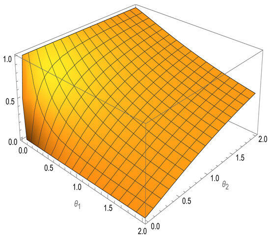
Figure 4. The SSR of iXgamma for different values of ${\theta }_1$ and ${\theta }_2$.

3. Non-Bayesian Estimation

In this section, we will discuss the non-Bayesian methods for estimating the unknown parameter $\theta$ of the iXgamma distribution in the presence of PCT-II censoring, specifically, MLE and MPS.

3.1. Maximum Likelihood Estimation

Here, we estimate the parameter $\theta$ of the iXgamma distribution under PCT-II samples using the MLE. Let $x_{\left(1\right)},x_{\left(2\right)},\cdots ,x_{\left(m\right)}$ where $1\le m\le n$ is the PCT-II sample of size m from a sample of n with the scheme $R_1,R_2,\dots ,R_m$, drawn from the iXgamma distribution with parameter $\theta$. Substituting the Cdf and Pdf from Equations (5) and (6), respectively, into Equation (1), the log-likelihood function of $\theta$ can be given as follows:

$$L\left(\theta \right)\propto \prod _{i=1}^m\left({\displaystyle \frac{\theta }{3+\theta }}\left(1+\theta +\theta x_{\left(i\right)}+0.5{\theta }^2{x}_{\left(i\right)}^2\right)e^{-\theta x_{\left(i\right)}}\right)\times {\left(\left[1+{\displaystyle \frac{\theta }{\theta +3}}\left(2x_{\left(i\right)}+0.5\theta x_{\left(i\right)}^2\right)\right]e^{-\theta x_{\left(i\right)}}\right)}^{R_i}.$$

(7)

The log-likelihood function $(\ell )$, without the constant term, can be written as follows:

$$\begin{array}{cc}\hfill \ell & =mln\left({\displaystyle \frac{\theta }{\theta +3}}\right)-\theta \sum _{i=1}^m{x}_{\left(i\right)}+\sum _{i=1}^{m}ln\left(1+\theta +\theta x_{\left(i\right)}+0.5{\theta }^2{x}_{\left(i\right)}^2\right)+\hfill \\ \hfill & \sum _{i=1}^m{R}_{i}ln\left(1+{\displaystyle \frac{\theta }{\theta +3}}\left(2x+0.5\theta x_{\left(i\right)}^2\right)\right)-\theta \sum _{i=1}^m{R}_i{x}_{\left(i\right)},\hfill \end{array}$$

(8)

Calculating the first partial derivatives of ℓ with respect to $\theta$, and equating each to zero, we obtain the likelihood equations as follows:

$$\begin{array}{cc}\hfill {\displaystyle \frac{\partial \ell }{\partial \theta }}& ={\displaystyle \frac{3m}{\theta (\theta +3)}}-\sum _{i=1}^m{x}_{\left(i\right)}+\sum _{i=1}^m\left({\displaystyle \frac{1+x_{\left(i\right)}+\theta x_{\left(i\right)}^2}{1+\theta +\theta x_{\left(i\right)}+0.5{\theta }^2{x}_{\left(i\right)}^2}}\right)\hfill \\ \hfill & +\sum _{i=1}^m{R}_i{\displaystyle \frac{x_{\left(i\right)}(\theta (\theta +6)x_{\left(i\right)}+12)}{(\theta +3)({\theta }^2{x}_{\left(i\right)}^2+\theta (4x_{\left(i\right)}+2)+6)}}-\sum _{i=1}^m{R}_i{x}_{\left(i\right)}=0.\hfill \end{array}$$

(9)

Since Equation (9) does not provide any closed-form solutions, we use the Newton–Raphson iteration method by using the optim() command of the R programming software to obtain the estimates. Refs. [4,14,18] describe the algorithm as follows:

• Initially, set $k=0$ and use ${\theta }_0$ as the starting point of iteration.
• Calculate ${\left({\displaystyle \frac{\partial \ell }{\partial \theta }}\right)}_{\left({\theta }_k\right)}$, where ${\theta }_k$ is the value of the unknown parameter $\theta$ at iteration number k and find the observed Fisher information matrix $I^{-1}\left(\theta \right)$.
• Then, continue the iteration with $\theta$ as follows:

  $${\theta }_{k+1}={\theta }_k+{\left({\displaystyle \frac{\partial \ell }{\partial \theta }}\right)}_{\left({\theta }_k\right)}\times I^{-1}\left(\theta \right),$$

  where $I^{-1}\left(\theta \right)=-E\left[\left({\displaystyle \frac{{\partial }^2\ell }{\partial {\theta }^2}}\right)\right]$; the Fisher information matrix can also be obtained from the second-order partial derivatives of the log-likelihood function.
• Increment $k=k+1$ and return to Step 2.
• Continue the iterative steps until $\left|{\theta }_{k+1}-{\theta }_k\right|$ is smaller than a threshold value. The final estimates of $\theta$ are the MLE of the parameters, denoted as $\widehat{\theta }$.

Moreover, using the invariance property of the MLEs, we obtain the MLEs of $R\left(x\right)$ and $r\left(x\right)$ by replacing $\theta$ with $\widehat{\theta }$, as follows:

$$\begin{array}{cc}\hfill \widehat{R}\left(x\right)& =\left[1+{\displaystyle \frac{\widehat{\theta }}{\widehat{\theta }+3}}(2x+{\displaystyle \frac{\widehat{\theta }{x}^2}{2}})\right]e^{-\widehat{\theta }x}\hfill \\ \hfill \widehat{r}\left(x\right)& ={\displaystyle \frac{\widehat{\theta }\left(1+\widehat{\theta }+\widehat{\theta }x+{\displaystyle \frac{{\widehat{\theta }}^2{x}^2}{2}}\right)}{\left(3+\widehat{\theta }+2\widehat{\theta }x+{\displaystyle \frac{{\widehat{\theta }}^2{x}^2}{2}}\right)}}.\hfill \end{array}$$

Existence and Uniqueness of MLEs

To check the existence and uniqueness of $\widehat{\theta }$ under the PCT-II sample data, we begin by taking the second partial derivatives of the log-likelihood function ℓ with respect to $\theta$ as follows:

$$\begin{array}{cc}\hfill {\displaystyle \frac{{\partial }^2\ell }{\partial {\theta }^2}}& =-\sum _{i=1}^m{R}_i{\displaystyle \frac{x_{\left(i\right)}\left(48(\theta +3)+{\theta }^2\left({\theta }^2+12\theta +18\right)x_{\left(i\right)}^3+24\theta (2\theta +3)x_{\left(i\right)}^2+12(5\theta +3)x_{\left(i\right)}\right)}{{(\theta +3)}^2{\left({\theta }^2{x}_{\left(i\right)}^2+\theta (4x_{\left(i\right)}+2)+6\right)}^2}}\hfill \\ \hfill & -\sum _{i=1}^m{\displaystyle \frac{2\left({\theta }^2{x}_{\left(i\right)}^4+2\theta x_{\left(i\right)}^3+2\theta x_{\left(i\right)}^2+4x_{\left(i\right)}+2\right)}{{\left({\theta }^2{x}_{\left(i\right)}^2+2\theta (x_{\left(i\right)}+1)+2\right)}^2}}-{\displaystyle \frac{3m(3+2\theta )}{{\theta }^2{(3+\theta )}^2}}.\hfill \end{array}$$

(10)

From Equation (10), one can observe that

$${\displaystyle \frac{{\partial }^2\ell }{\partial {\theta }^2}}<0,$$

which is a clear indication that the log-likelihood function ℓ is strictly concave. So, we can say that the MLE exists and is unique.

3.2. Maximum Product Spacing

The maximum product spacing (MPS) method, which approximates the Kullback–Leibler information measure, serves as a reliable alternative to the MLE method. Consider the PCT-II sample of size m, obtained using the PCT-II scheme from the iXgamma population with parameter $\theta$, denoted as $x=x_{\left(i\right)}$, where i ranges from 1 to m. The MPS for the iXgamma distribution can be formulated as follows:

$$\begin{array}{cc}\hfill GS\left(\theta \right)& =\prod _{i=1}^{m+1}\left(F\left(x_{\left(i\right)}\right)-F\left(x_{(i-1)}\right)\right)\prod _{i=1}^m{(1-F\left(x_{\left(i\right)}\right))}^{R_i}\hfill \\ \hfill & =\prod _{i=1}^{m+1}\left(\left[1+{\displaystyle \frac{\theta }{\theta +3}}\left(2x_{(i-1)}+{\displaystyle \frac{\theta x_{(i-1)}^2}{2}}\right)\right]e^{-\theta x_{(i-1)}}-\left[1+{\displaystyle \frac{\theta }{\theta +3}}\left(2x_{\left(i\right)}+{\displaystyle \frac{\theta x_{\left(i\right)}^2}{2}}\right)\right]e^{-\theta x_{\left(i\right)}}\right)\hfill \\ \hfill & \prod _{i=1}^m{\left(\left[1+{\displaystyle \frac{\theta }{\theta +3}}\left(2x_{\left(i\right)}+{\displaystyle \frac{\theta x_{\left(i\right)}^2}{2}}\right)\right]e^{-\theta x_{\left(i\right)}}\right)}^{R_i},\hfill \end{array}$$

(11)

and $gs\left(\theta \right)=ln\left(Gs\right(\theta \left)\right)$ can be obtained as

$$\begin{array}{cc}\hfill gs\left(\theta \right)& =\sum _{i=1}^{m+1}ln\left(\left[1+{\displaystyle \frac{\theta }{\theta +3}}\left(2x_{(i-1)}+{\displaystyle \frac{\theta x_{(i-1)}^2}{2}}\right)\right]e^{-\theta x_{(i-1)}}-\left[1+{\displaystyle \frac{\theta }{\theta +3}}\left(2x_{\left(i\right)}+{\displaystyle \frac{\theta x_{\left(i\right)}^2}{2}}\right)\right]e^{-\theta x_{\left(i\right)}}\right)\hfill \\ \hfill & +R_i\sum _{i=1}^{m}ln\left(\left[1+{\displaystyle \frac{\theta }{\theta +3}}\left(2x_{\left(i\right)}+{\displaystyle \frac{\theta x_{\left(i\right)}^2}{2}}\right)\right]e^{-\theta x_{\left(i\right)}}\right)\hfill \end{array}$$

(12)

Upon deriving the first derivative of the function $gs\left(\theta \right)$ with respect to $\theta$, we obtain:

$$\begin{array}{cc}\hfill {\displaystyle \frac{\partial gs\left(\theta \right)}{\partial \theta }}& ={\displaystyle \frac{{\sum }_{i=1}^{m+1}\left(\left[\frac{x_{\left(i\right)}(\theta x_{\left(i\right)}(\theta ((\theta +3)x_{\left(i\right)}+3)+6)-12)}{(\theta +3)\left(2(\theta +3)e^{\theta x_{\left(i\right)}}+\theta x_{\left(i\right)}(\theta x_{\left(i\right)}+4)\right)}\right)-\left[\frac{x_{(i-1)}(\theta x_{(i-1)}(\theta ((\theta +3)x_{(i-1)}+3)+6)-12)}{(\theta +3)\left(2(\theta +3)e^{\theta x_{(i-1)}}+\theta x_{(i-1)}(\theta x_{(i-1)}+4)\right)}\right]\right)}{{\sum }_{i=1}^{m+1}ln\left(\left[1+\frac{\theta }{\theta +3}\left(2x_{(i-1)}+\frac{\theta x_{(i-1)}^2}{2}\right)\right]e^{-\theta x_{(i-1)}}-\left[1+\frac{\theta }{\theta +3}\left(2x_{\left(i\right)}+\frac{\theta x_{\left(i\right)}^2}{2}\right)\right]e^{-\theta x_{\left(i\right)}}\right)}}\hfill \\ \hfill & +\sum _{i=1}^m{R}_i\left[{\displaystyle \frac{x_{\left(i\right)}(\theta x_{\left(i\right)}(\theta ((\theta +3)x_{\left(i\right)}+3)+6)-12)}{(\theta +3)\left(2(\theta +3)e^{\theta x_{\left(i\right)}}+\theta x_{\left(i\right)}(\theta x_{\left(i\right)}+4)\left(\left[1+\frac{\theta }{\theta +3}\left(2x_{\left(i\right)}+\frac{\theta x_{\left(i\right)}^2}{2}\right)\right]e^{-\theta x_{\left(i\right)}}\right)\right)}}\right]\hfill \end{array}$$

(13)

Setting Equation (13) equal to zero and solving for $\theta$, the MPS is obtained. Equation (13) does not provide a closed-form analytical solution when equated to zero. Consequently, numerical methods are employed to find the solutions.

4. Bayesian Estimation

In this section, we derive the Bayesian estimation (BE) of the parameter $\theta$ for the iXgamma distribution under PCT-II samples, assuming a Gamma prior distribution. The Gamma prior is specified as follows:

$$\pi \left(\theta \right)\propto {\theta }^{a-1}{e}^{-b\theta },\theta >0,a>0,b>0.$$

Thus, the posterior distribution is given by:

$${\pi }^{*}\left(\theta \mid \mathbf{x}\right)={\displaystyle \frac{\pi \left(\theta \right)L\left(\theta \right)}{{\int }_0^{\infty }\pi \left(\theta \right)L\left(\theta \right)d\theta }},$$

(14)

where $L\left(\theta \right)$ is the likelihood function given in Equation (7) based on the PCT-II samples (x̠). The integral in the denominator ensures that the posterior distribution is normalized. Thus, the posterior distribution can be written

$$\begin{array}{cc}\hfill {\pi }^{*}\left(\theta \mid \underset{-}{\mathrm{x}}\right)& \propto \prod _{i=1}^m\left[{\theta }^{a-1}{\mathrm{e}}^{-b\theta }\right].\prod _{i=1}^m\left({\displaystyle \frac{\theta }{3+\theta }}\left(1+\theta +\theta x_i+{\displaystyle \frac{{\theta }^2{x}_i^2}{2}}\right)e^{-\theta x_i}\right)\hfill \\ \hfill & \times {\left(1+{\displaystyle \frac{\theta }{\theta +3}}\left(2x_i+{\displaystyle \frac{\theta x_i^2}{2}}\right)e^{-\theta x_i}\right)}^{R_i}\hfill \end{array}$$

A commonly used symmetrical loss function is the square error loss (SEL), which assigns equal losses to overestimation and underestimation. If $l\left(\theta \right)$ is estimated by an estimator $\widehat{l}\left(\theta \right)$, then the SEL function is defined as

$$E\left(l\left(\theta \right),\widehat{l}\left(\theta \right)\right)=E{\left(l\left(\theta \right)-\widehat{l}\left(\theta \right)\right)}^2.$$

Therefore, the BE of any function of $\theta$, say $l\left(\theta \right)$ under the SEL function, can be obtained as

$${\widehat{\theta }}_{SEL}=E\left[l\left(\theta \right)|\mathbf{x}\right]={\int }_{\theta }l\left(\theta \right)\pi \left(\theta \right|x)d\theta .$$

(15)

Ref. [28] considered a LINEX (linear-exponential) loss function $L\left(▵\right)$ for a parameter $\theta$ is given by

$$L\left(▵\right)=\left(e^{c▵}-c▵-1\right),c\ne 0,▵=\widehat{\theta }-\theta .$$

This loss function is suitable for situations where overestimation is more costly than underestimation. Ref. [29] discussed BE and prediction using the LINEX loss. Hence, under the LINEX loss function, the BE of a function $l\left(\theta \right)$ is

$${\widehat{\theta }}_{LINEX}=-{\displaystyle \frac{1}{c}}ln\left[E\left(e^{-cl\left(\theta \right)}\mid \underset{-}{\mathrm{x}}\right)\right],c\ne 0,$$

(16)

The BE of a function of $ł\left(\theta \right)$, concerning the general entropy loss (GEL) function, is given by

$${\widehat{\theta }}_{GEL}={\left[E\left(l{\left(\theta \right)}^{-p}\right|\underset{-}{\mathrm{x}})\right]}^{-1/p},p\ne 0$$

(17)

All the above estimators in Equations (15)–(17) are the form of the ratio of two integrals for which simplified closed forms are not available. The Tierney–Kadan method is a numeric integration technique in such cases, and the Markov Chain Monte Carlo (MCMC) method finds the BEs.

4.1. MCMC Method

The MCMC methodology is one of the most effective numerical approaches in Bayesian inference. Moreover, calculating the normalization constant is unnecessary when summarizing the posterior distribution using MCMC methods. MCMC techniques have been extensively utilized in Bayesian statistical inference [32,33,34,35,36]. An algorithm, the Metropolis–Hastings (MH) algorithm, can be utilized as a sampler for the MCMC approach. A critical aspect of this method involves selecting an appropriate proposal distribution that satisfies two key criteria: (1) it should be easy to simulate, and (2) it should closely approximate the posterior distribution of interest. Once such a proposal distribution is identified, the acceptance/rejection rule is employed to generate random samples from the target posterior distribution. This enables efficient approximation of the Bayesian posterior summaries.

After obtaining a set of M samples from the posterior distribution, discarding a portion of the initial samples (known as the burn-in samples), and retaining the remaining samples for further analysis is common practice. Specifically, the BEs of the parameter $\theta$, using the SEL and LINEX, GEL functions, are provided as follows:

$$\begin{array}{cc}\hfill {\widehat{\theta }}_{\mathrm{MCMC}:\mathrm{SEL}}& ={\displaystyle \frac{1}{M-I_B}}\sum _{i=I_B+1}^M{\theta }_i\hfill \end{array}$$

(18)

$$\begin{array}{cc}\hfill {\widehat{\theta }}_{\mathrm{MCMC}:\mathrm{LINEX}}& =-{\displaystyle \frac{1}{c}}ln\left({\displaystyle \frac{1}{M-I_B}}\sum _{i=I_B+1}^M{e}^{-c{\theta }_i}\right)\hfill \end{array}$$

(19)

$$\begin{array}{cc}\hfill {\widehat{\theta }}_{\mathrm{MCMC}:\mathrm{GEL}}& ={\left({\displaystyle \frac{1}{M-I_B}}\sum _{i=I_B+1}^M{\theta }_i^{-p}\right)}^{-1/p}\hfill \end{array}$$

(20)

where $I_B$ represents the number of burn-in samples.

MCMC Convergence

The Gelman–Rubin statistics are available to assess the convergence of the samples produced by the posterior distribution using MCMC. The goal of this approach is to confirm that MCMC samples have reached the target distribution that was planned for them. In this work, we use several Markov chains to evaluate convergence using the Gelman–Rubin statistic, which is sometimes referred to as the potential scale reduction factor (PSRF). The following formula is used to determine the PSRF:

$$\mathrm{PSRF}=\sqrt{{\displaystyle \frac{\frac{M-1}{M}{V}_w+\frac{1}{M}{V}_b}{V_w}}}$$

(21)

where $V_w$ is the average within-chain variance, and the term in the numerator combines the between-chain variance $V_b$ with the within-chain variance $V_w$ to estimate the marginal posterior variance of the parameter. The number of iterations of each chain is shown here by M.

It is likely that the chains have converged if the PSRF value is near 1. The Gelman–Rubin statistic is extremely valuable as it uses several chains to provide an independent measure of convergence, eliminating the potential of erroneous integration that usually exists when using only a single chain. For more information, see [37].

4.2. Tierney–Kadane Method

Here, in this method, the ratios of the integrals from Equations (15)–(17) are represented in two forms shown below:

$$\begin{array}{c}\hfill H\left(\theta \right)={\displaystyle \frac{1}{n}}\pi \left(\theta \right|\mathbf{x})\end{array}$$

(22)

$$\begin{array}{c}\hfill H^{*}\left(\theta \right)=H\left(\theta \right)+{\displaystyle \frac{1}{n}}lng\left(\theta \right)\end{array}$$

(23)

$$\begin{array}{ccc}\hfill H\left(\theta \right)& =& {\displaystyle \frac{1}{n}}\left((a-1)ln\theta -b\theta +mln{\displaystyle \frac{\theta }{\theta +3}}-\theta m\overline{x}+\sum _{i=1}^{m}ln\left(1+\theta +\theta x_i+{\displaystyle \frac{{\theta }^2{x}_i^2}{2}}\right)\right)\hfill \\ & +& {\displaystyle \frac{1}{n}}\left(\sum _{i=1}^m{R}_{i}ln\left(1+{\displaystyle \frac{\theta }{\theta +3}}(2x+{\displaystyle \frac{\theta x_i^2}{2}})\right)-\theta \sum _{i=1}^m{R}_i{x}_i\right).\hfill \end{array}$$

(24)

The equation takes the form of

$$\begin{array}{c}\hfill \widehat{{\theta }_{TK}}=\sqrt{{\displaystyle \frac{|{\sum }^{*}|}{|\sum |}}}g\left(\widetilde{{\theta }^{*}}\right){\displaystyle \frac{\pi \left(\widetilde{{\theta }^{*}}\right|\mathbf{x})}{\pi \left(\tilde{\theta }\right|\mathbf{x})}},\end{array}$$

(25)

where $\widetilde{{\theta }^{*}}$ and $\tilde{\theta }$ maximize $H^{*}\left(\theta \right)$ and $H\left(\theta \right)$, respectively, and $|{\sum }^{*}|$ and $|\sum |$ are the negatives of the inverse Hessian of $H^{*}\left(\theta \right)$ and $H\left(\theta \right)$ at $\widetilde{{\theta }^{*}}$ and $\tilde{\theta }$, respectively. Here, Equation (25) is used to obtain the Bayes estimators for the parameter $\theta$, which is an approximation form. Now, differentiating Equation (24) with respect to $\theta$, we obtain,

$$\begin{array}{ccc}\hfill H_1& =& {\displaystyle \frac{\partial H\left(\theta \right)}{\partial \theta }}={\displaystyle \frac{1}{n}}\left[{\displaystyle \frac{a-1}{\theta }}-b+{\displaystyle \frac{3m}{\theta (\theta +3)}}-m\overline{x}+\sum _{i=1}^m{\displaystyle \frac{1+x_i+\theta x_i^2}{1+\theta +\theta x_i+{\displaystyle \frac{{\theta }^2{x}_i^2}{2}}}}\right]\hfill \\ & & {\displaystyle \frac{1}{n}}\left[\sum _{i=1}^m{R}_i{x}_i+\sum _{i=1}^m{R}_i\left({\displaystyle \frac{{\displaystyle \frac{\theta x_i^2}{2}}+{\displaystyle \frac{3(2x_i+\theta /2x_i^2)}{(\theta +3)}}}{\theta +3+\theta (2x_i+\theta /2x_i^2)}}\right)\right].\hfill \end{array}$$

Now, the BE of $\theta$ can be computed as follows:

4.2.1. Under SEL Function

If $l\left(\theta \right)=\theta$, then the Equation (22) becomes

$${}_{\theta }H^{*}\left(\theta \right)=H\left(\theta \right)+{\displaystyle \frac{ln\theta }{n}}.$$

The first derivatives of ${}_{\theta }H^{*}\left(\theta \right)$ with respect to $\theta$ is

$${\displaystyle \frac{{\partial }_{\theta }{H}^{*}\left(\theta \right)}{\partial \theta }}{=}_{\theta }{H}_1^{*}\left(\theta \right)=H^{\prime }\left(\theta \right)+{\displaystyle \frac{1}{n\theta }}$$

Again differentiating with respect to $\theta$, we obtain

$$\begin{array}{c}\hfill {\displaystyle \frac{{\partial }_{\theta }^2{H}^{*}\left(\theta \right)}{\partial {\theta }^2}}{=}_{\theta }{H}_{11}^{*}\left(\theta \right)=H^{\prime \prime }\left(\theta \right)-{\displaystyle \frac{1}{n{\theta }^2}}\end{array}$$

Therefore,

$$\sum ={\displaystyle \frac{1}{H^{\prime \prime }\left(\theta \right)-{\displaystyle \frac{1}{n{\theta }^2}}}}$$

Putting the value in Equation (25), we obtain the Bayes estimator using the TK method under the SEL function.

4.2.2. Under the LINEX Function

If $l\left(\theta \right)=e^{-c\theta }$, then the Equation (22) becomes

$${}_{\theta }H^{*}\left(\theta \right)=H\left(\theta \right)-{\displaystyle \frac{1}{n}}c\theta .$$

The first derivative of ${}_{\theta }H^{*}\left(\theta \right)$ with respect to $\theta$ is

$${\displaystyle \frac{{\partial }_{\theta }{H}^{*}\left(\theta \right)}{\partial \theta }}{=}_{\theta }{H}_1^{*}\left(\theta \right)=H^{\prime }\left(\theta \right)-{\displaystyle \frac{c}{n}}$$

Again differentiating with respect to $\theta$, we obtain

$$\begin{array}{c}\hfill {\displaystyle \frac{{\partial }_{\theta }^2{H}^{*}\left(\theta \right)}{\partial {\theta }^2}}{=}_{\theta }{H}_{11}^{*}\left(\theta \right)=H^{\prime \prime }\left(\theta \right)\end{array}$$

Therefore,

$$\sum ={\displaystyle \frac{1}{H^{\prime \prime }\left(\theta \right)}}$$

Putting the value in Equation (25), we obtain the Bayes estimator using the TK method under the LINEX function.

4.2.3. Under the GEL Function

If $l\left(\theta \right)={\theta }^{-p}$, then the Equation (22) becomes

$${}_{\theta }H^{*}\left(\theta \right)=H\left(\theta \right)-{\displaystyle \frac{pln\theta }{n}}.$$

The first derivative of ${}_{\theta }H^{*}\left(\theta \right)$ with respect to $\theta$ is

$${\displaystyle \frac{{\partial }_{\theta }{H}^{*}\left(\theta \right)}{\partial \theta }}{=}_{\theta }{H}_1^{*}\left(\theta \right)=H^{\prime }\left(\theta \right)-{\displaystyle \frac{p}{n\theta }}$$

Again differentiating with respect to $\theta$, we obtain

$$\begin{array}{c}\hfill {\displaystyle \frac{{\partial }_{\theta }^2{H}^{*}\left(\theta \right)}{\partial {\theta }^2}}{=}_{\theta }{H}_{11}^{*}\left(\theta \right)=H^{\prime \prime }\left(\theta \right)+{\displaystyle \frac{p}{n{\theta }^2}}\end{array}$$

Therefore,

$$\sum ={\displaystyle \frac{1}{H^{\prime \prime }\left(\theta \right)+{\displaystyle \frac{p}{n{\theta }^2}}}}$$

Putting the value in Equation (25), we obtain the Bayes estimator using the TK method under the GEL function.

5. Confidence Interval Estimation

The confidence interval (CI) estimation for the parameter $\theta$ is derived from data obtained from the iXgamma distribution under the PCT-II scheme. In this section, the asymptotic confidence intervals and the highest posterior density intervals for the MLEs and BEs are presented.

5.1. Approximate Confidence Interval

Approximate confidence interval (ACI) estimation for the parameter $\theta$ using large-sample approximations. Two methods are presented: normal approximation (NA), which assumes $\theta$ follows a normal distribution, and log-transformed normal approximation (NL), which applies a logarithmic transformation for better coverage. The NA method provides direct ACI estimates, while the NL method ensures a more reliable range, especially for small samples or highly skewed distributions

5.2. Highest Posterior Density

According to the technique of [34], one can establish the highest posterior density (HPD) intervals for the unknown parameter $\theta$ of the iXgamma distribution under the PCT-II scheme using the samples obtained by the suggested MH algorithm in the preceding paragraph. Considering ${\theta }^{\left(\gamma \right)}$ to be the $\gamma$th quantile of $\theta$, that is,

$${\theta }^{\left(\gamma \right)}=inf\{\theta :\Pi \left(\theta \mid \mathbf{x}\right)\ge \gamma \},$$

where $0<\gamma <1$ and $\Pi (·)$ is the posterior function of $\theta$. It should be noted that for a given ${\theta }^{*}$, an accurate estimator based on simulation of $\pi \left(\theta \mid \mathbf{x}\right)$ might well be computed as

$$\Pi \left\{\theta \mid \mathbf{x}\right\}={\displaystyle \frac{1}{M-l_B}}\sum _{i=l_B}^M{I}_{\theta \le {\theta }^{*}}.$$

Here, $I_{\theta \le {\theta }^{*}}$ is the indicator function. The proper estimate is then determined as

$$\widehat{\Pi }\left({\theta }^{*}\mid \mathbf{x}\right)=\left\{\begin{array}{cc}0\hfill & if{\theta }^{*}<{\theta }_{l_B}\hfill \\ \sum _{j=l_B}^i{\omega }_j\hfill & if{\theta }_i<{\theta }^{*}<{\theta }_{i+1}\hfill \\ 1\hfill & if{\theta }^{*}>{\theta }_M\hfill \end{array}\right.$$

where ${\omega }_j={\displaystyle \frac{1}{M-l_B}}$ and ${\theta }^j$ are the ordered values of ${\theta }^{\left(j\right)}$. Now, for $i=l_B,\dots ,M$, ${\theta }^{\left(\gamma \right)}$ may be estimated by

$${\tilde{\theta }}^{\left(\gamma \right)}=\left\{\begin{array}{cc}{\theta }_{l_B}\hfill & if\gamma =0\hfill \\ {\theta }_i\hfill & if\sum _{j=l_B}^{i-1}{\omega }_j<\gamma <\sum _{j=l_B}^i{\omega }_j.\hfill \end{array}\right.$$

Let determine a $100(1-\gamma )\%$ HPD credible interval for $\theta$ as

$$HP{D}_j^{\theta }=\left({\tilde{\theta }}^{\left({\displaystyle \frac{j}{M}}\right)},{\tilde{\theta }}^{\left({\displaystyle \frac{j+(1-\gamma )M}{M}}\right)}\right)$$

for $j=l_B,\dots ,\left[\gamma M\right]$; here, $\left[a\right]$ indicates the largest integer that ≤a. It is necessary to choose $HP{D}_{j^{*}}$ from one of many $HP{D}_j^{\theta }$s with the narrowest width.

6. Simulation Study and Discussion

In this section, Monte Carlo simulation studies are conducted to evaluate the performance of various estimation methods, including MLE, MPS, and BE, within the framework of the PCT-II scheme for the iXgamma distribution. We produce 1000 data points from the iXgamma distribution with parameters $\theta =0.5,1.5,$ and 3. The choice of parameter values for the iXgamma distribution covered different shapes and behaviors of the distribution, allowing for an analysis of its behavior under these values. The PCT-II scheme can be assumed according to a given value of n and m and a different pattern for removing items $R_i$, where $i=1,2,\dots ,m$, as shown in Table 2.

Table 2. Proposed schemes for PCT-II.

n	m	CS
		${\mathcal{R}}_{\mathbf{1}}$	${\mathcal{R}}_{\mathbf{2}}$	${\mathcal{R}}_{\mathbf{3}}$	${\mathcal{R}}_{\mathbf{4}}$	${\mathcal{R}}_{\mathbf{5}}$
30	10	$\left(20,0^{*9}\right)$	$\left(10,0^{*8},10\right)$	$\left(0^{*4},10,10,0^{*4}\right)$	$\left(0^{*9},20\right)$	$\left(2^{*10}\right)$
	20	$\left(10,0^{*19}\right)$	$\left(5,0^{*18},5\right)$	$\left(0^{*9},5,5,0^{*9}\right)$	$\left(0^{*19},10\right)$	$\left(1^{*10},0^{*10}\right)$
60	20	$\left(40,0^{*19}\right)$	$\left(20,0^{*18},20\right)$	$\left(0^{*9},20,20,0^{*9}\right)$	$\left(0^{*19},40\right)$	$\left(2^{*20}\right)$
	40	$\left(20,0^{*39}\right)$	$\left(10,0^{*38},10\right)$	$\left(0^{*19},10,10,0^{*19}\right)$	$\left(0^{*39},20\right)$	$\left(1^{*20},0^{*20}\right)$

Here, $(0^{*4},10)$, for instance, represents a censoring scheme expressed as $(0,0,0,0,10)$.

This implies that the scheme ${\mathcal{R}}_4$ corresponds to a Type-II censoring scheme as a particular case, with the number of failure items given by $R_m=n-m$. Moreover, complete sampling is treated as a special case of the PCT-II scheme when $R_i=0$ for $i=1,2,\dots ,n$.

6.1. Monte Carlo Simulation Process

• Generate random samples for the iXgamma distribution with parameter $\theta$ using the assumed schemes of PCT-II in Table 2 employing the algorithm proposed by [2].
• Estimate the parameter $\theta$ using non-Bayesian methods (Non-BE), specifically MLE and MPS. From the MLE, the variance of the parameter $\theta$ can also be derived. When calculating MLEs, the initial estimate values are assumed to coincide with the true parameter values.
• Estimate the parameter $\theta$ using Bayesian methods (BE) as follows:

  (a)

  Assume the informative prior case, where the hyper-parameters are proposed and fixed at $a=1.5$ and $b=2.5$. These values are plugged into the posterior density.

  (b)

  Consider three loss functions: SEL, LINEX (with $c=1.5$), and GEL (with $p=-0.5$). We have experimented with different values to achieve the best possible results through these functions, ultimately arriving at the current values.

  (c)

  Estimate the parameter $\theta$ using the BE methods adopted in the research, initially through the TK method and MCMC.

  (d)

  For the MCMC method, using the MH algorithm:

  • The initial values for the MH algorithm are set to the MLE estimates with their variances.
  • Proposal samples for $\theta$ are generated from a normal distribution: $\theta \sim N(\widehat{\theta },I^{-1}\left(\widehat{\theta }\right))$, where $\widehat{\theta }$ is the MLE of $\theta$, and $I\left(\widehat{\theta }\right)$ is the observed Fisher information matrix of $\theta$.
  • A total of 10,000 posterior samples are generated, with the first 2000 samples discarded as burn-in to enhance the convergence of the MCMC estimation.
  • The final estimate of $\theta$ is obtained by computing the average based on the chosen loss functions.
  • The acceptance rate in our MCMC implementation was approximately 65%.

• Estimate the CIs for the parameter $\theta$, which are the NA, NL, and HPD intervals.
• Perform steps 1 to 4 iteratively for a total of 1000 repetitions, storing all resulting estimates. Subsequently, compute the average (AV) and root mean square error (RMSE) for the point estimate. Additionally, determine the mean values of the lower and upper bounds of the CIs, calculate the average interval length (AIL), and evaluate the coverage probability (CP) as a percentage (%).
• In addition to the specific PCT-II patterns in Table 2, a general case of complete sampling has been added to estimates where $m=n$ and did not involve the exclusion of units from the experiment.

6.2. Comments on Results

In Table 3, Table 4 and Table 5,we obtained point estimates for the parameter $\theta$ at values 0.5, 1.5, and 2.5, respectively, for all estimation methods. Meanwhile, in Table 6, Table 7 and Table 8, we obtained interval estimates for the same parameter values in the same sequence. In general, from the results, we observe that as m increases, there is an improvement in the estimates converging closer to the assumed parameter value. Additionally, we observe a decrease in RMSE and, finally, a decrease in AILs for all estimation methods. Furthermore, CP is also observed to be constrained within specific bounds greater than 94%. There are also specific observations regarding the patterns of PCT-II and estimation methods, which can be summarized as follows:

Table 3. The estimated values of AV and RMSE under various PCT-II schemes at $\theta =0.5$.

n	m	CS		Non-BE		BE: TK			BE: MCMC
				MLE	MPS	SEL	LINEX	GEL	SEL	LINEX	GEL
30	10	${\mathcal{R}}_1$	AV	0.5444	0.5862	0.5031	0.4568	0.4948	0.4599	0.4410	0.5164
			RMSE	0.1617	0.1927	0.1343	0.1258	0.1321	0.1686	0.1620	0.1397
		${\mathcal{R}}_2$	AV	0.5418	0.5117	0.5011	0.4530	0.4925	0.4539	0.4262	0.5113
			RMSE	0.1543	0.1407	0.1288	0.1226	0.1269	0.1675	0.1715	0.1352
		${\mathcal{R}}_3$	AV	0.5404	0.5654	0.4992	0.4518	0.4907	0.4560	0.4267	0.5093
			RMSE	0.1504	0.1711	0.1260	0.1211	0.1243	0.1665	0.1613	0.1323
		${\mathcal{R}}_4$	AV	0.5429	0.5065	0.5010	0.4518	0.4922	0.4382	0.4158	0.5113
			RMSE	0.1586	0.1429	0.1317	0.1253	0.1298	0.1775	0.1744	0.1349
		${\mathcal{R}}_5$	AV	0.5419	0.5198	0.5007	0.4526	0.4921	0.4494	0.4213	0.5108
			RMSE	0.1630	0.1523	0.1360	0.1284	0.1339	0.1688	0.1707	0.1415
	20	${\mathcal{R}}_1$	AV	0.5179	0.5447	0.4990	0.4766	0.4949	0.5105	0.5040	0.5066
			RMSE	0.0991	0.1141	0.0912	0.0890	0.0906	0.0942	0.0913	0.0931
		${\mathcal{R}}_2$	AV	0.5152	0.5113	0.4969	0.4745	0.4928	0.5078	0.5015	0.5039
			RMSE	0.0952	0.0938	0.0880	0.0867	0.0875	0.0908	0.0881	0.0898
		${\mathcal{R}}_3$	AV	0.5156	0.5379	0.4967	0.4741	0.4927	0.5082	0.5017	0.5041
			RMSE	0.0998	0.1103	0.0923	0.0907	0.0918	0.0947	0.0917	0.0937
		${\mathcal{R}}_4$	AV	0.5202	0.5107	0.5015	0.4786	0.4974	0.5117	0.5048	0.5080
			RMSE	0.1030	0.0996	0.0945	0.0914	0.0937	0.0977	0.0957	0.0963
		${\mathcal{R}}_5$	AV	0.5201	0.5448	0.5010	0.4783	0.4970	0.5110	0.5048	0.5084
			RMSE	0.0984	0.1124	0.0902	0.0876	0.0895	0.0941	0.0916	0.0921
	Complete		AV	0.5110	0.5296	0.4987	0.4839	0.4960	0.5067	0.5026	0.5041
			RMSE	0.0785	0.0863	0.0745	0.0734	0.0742	0.0761	0.0746	0.0755
60	20	${\mathcal{R}}_1$	AV	0.5138	0.5393	0.4951	0.4729	0.4911	0.5072	0.5005	0.5031
			RMSE	0.0950	0.1081	0.0882	0.0873	0.0878	0.0910	0.0897	0.0901
		${\mathcal{R}}_2$	AV	0.5182	0.5041	0.4994	0.4760	0.4952	0.5096	0.5029	0.5058
			RMSE	0.0986	0.0943	0.0908	0.0887	0.0902	0.0938	0.0913	0.0923
		${\mathcal{R}}_3$	AV	0.5139	0.5333	0.4950	0.4720	0.4909	0.5046	0.4986	0.5021
			RMSE	0.0901	0.0989	0.0836	0.0835	0.0833	0.0886	0.0854	0.0850
		${\mathcal{R}}_4$	AV	0.5220	0.5045	0.5024	0.4782	0.4980	0.5126	0.5048	0.5089
			RMSE	0.1039	0.0984	0.0949	0.0919	0.0942	0.0983	0.0964	0.0970
		${\mathcal{R}}_5$	AV	0.5186	0.5108	0.4997	0.4763	0.4955	0.5099	0.5030	0.5061
			RMSE	0.0980	0.0953	0.0901	0.0881	0.0895	0.0930	0.0909	0.0917
	40	${\mathcal{R}}_1$	AV	0.5090	0.5246	0.4999	0.4887	0.4979	0.5057	0.5027	0.5037
			RMSE	0.0649	0.0713	0.0623	0.0616	0.0621	0.0634	0.0625	0.0630
		${\mathcal{R}}_2$	AV	0.5097	0.5079	0.5008	0.4896	0.4988	0.5062	0.5031	0.5042
			RMSE	0.0669	0.0663	0.0641	0.0631	0.0639	0.0652	0.0642	0.0648
		${\mathcal{R}}_3$	AV	0.5107	0.5249	0.5015	0.4901	0.4994	0.5072	0.5040	0.5051
			RMSE	0.0693	0.0753	0.0663	0.0651	0.0660	0.0676	0.0664	0.0671
		${\mathcal{R}}_4$	AV	0.5089	0.5043	0.5000	0.4887	0.4979	0.5051	0.5020	0.5030
			RMSE	0.0626	0.0616	0.0601	0.0595	0.0599	0.0611	0.0602	0.0608
		${\mathcal{R}}_5$	AV	0.5136	0.5293	0.5042	0.4928	0.5021	0.5098	0.5066	0.5078
			RMSE	0.0688	0.0756	0.0655	0.0639	0.0651	0.0668	0.0655	0.0662
	Complete		AV	0.5083	0.5199	0.5022	0.4948	0.5009	0.5061	0.5040	0.5048
			RMSE	0.0562	0.0606	0.0544	0.0536	0.0542	0.0551	0.0545	0.0548

Table 4. The estimated values of AV and RMSE under various PCT-II schemes at $\theta =1.5$.

n	m	CS		Non-BE		BE: TK			BE: MCMC
				MLE	MPS	SEL	LINEX	GEL	SEL	LINEX	GEL
30	10	${\mathcal{R}}_1$	AV	1.6188	1.7270	1.3450	1.1672	1.3222	1.0978	0.8781	1.3801
			RMSE	0.4588	0.5327	0.3427	0.4132	0.3489	0.5694	0.7126	0.3458
		${\mathcal{R}}_2$	AV	1.6248	1.5345	1.3494	1.1691	1.3263	1.1017	0.8674	1.3803
			RMSE	0.4608	0.4203	0.3387	0.4107	0.3449	0.5538	0.7223	0.3445
		${\mathcal{R}}_3$	AV	1.6614	1.7392	1.3741	1.1900	1.3508	1.1135	0.8517	1.4091
			RMSE	0.5202	0.5767	0.3577	0.4095	0.3612	0.5493	0.7515	0.3621
		${\mathcal{R}}_4$	AV	1.6532	1.5452	1.3701	1.1861	1.3467	1.1153	0.9232	1.4021
			RMSE	0.4868	0.4344	0.3432	0.4047	0.3477	0.5561	0.6770	0.3430
		${\mathcal{R}}_5$	AV	1.6225	1.5566	1.3473	1.1675	1.3244	1.0726	0.8806	1.3832
			RMSE	0.4822	0.4503	0.3550	0.4204	0.3605	0.5865	0.7110	0.3551
	20	${\mathcal{R}}_1$	AV	1.5624	1.6388	1.4276	1.3308	1.4158	1.4631	1.4077	1.4546
			RMSE	0.3043	0.3478	0.2591	0.2795	0.2606	0.2622	0.2619	0.2592
		${\mathcal{R}}_2$	AV	1.5632	1.5491	1.4290	1.3318	1.4171	1.4644	1.4091	1.4546
			RMSE	0.3009	0.2955	0.2556	0.2765	0.2572	0.2594	0.2561	0.2571
		${\mathcal{R}}_3$	AV	1.5516	1.6151	1.4183	1.3221	1.4065	1.4553	1.3995	1.4450
			RMSE	0.3159	0.3491	0.2732	0.2935	0.2749	0.2737	0.2749	0.2731
		${\mathcal{R}}_4$	AV	1.5554	1.5262	1.4219	1.3251	1.4101	1.4579	1.3991	1.4462
			RMSE	0.3056	0.2958	0.2627	0.2845	0.2644	0.2628	0.2697	0.2669
		${\mathcal{R}}_5$	AV	1.5468	1.6152	1.4147	1.3190	1.4030	1.4469	1.3904	1.4415
			RMSE	0.3013	0.3381	0.2628	0.2864	0.2650	0.2681	0.2700	0.2618
	Complete		AV	1.5468	1.6019	1.4574	1.3909	1.4494	1.4845	1.4491	1.4764
			RMSE	0.2361	0.2607	0.2101	0.2199	0.2107	0.2117	0.2070	0.2113
60	20	${\mathcal{R}}_1$	AV	1.5580	1.6350	1.4239	1.3274	1.4121	1.4600	1.4047	1.4505
			RMSE	0.3082	0.3545	0.2640	0.2844	0.2656	0.2659	0.2668	0.2636
		${\mathcal{R}}_2$	AV	1.5575	1.5149	1.4239	1.3268	1.4121	1.4589	1.4071	1.4499
			RMSE	0.3047	0.2915	0.2620	0.2837	0.2637	0.2667	0.2589	0.2623
		${\mathcal{R}}_3$	AV	1.5511	1.6060	1.4196	1.3239	1.4079	1.4535	1.3996	1.4449
			RMSE	0.2952	0.3249	0.2575	0.2815	0.2594	0.2607	0.2628	0.2569
		${\mathcal{R}}_4$	AV	1.5405	1.4904	1.4104	1.3150	1.3987	1.4402	1.3929	1.4350
			RMSE	0.2951	0.2831	0.2614	0.2878	0.2638	0.2685	0.2635	0.2601
		${\mathcal{R}}_5$	AV	1.5565	1.5323	1.4239	1.3272	1.4121	1.4604	1.4065	1.4499
			RMSE	0.2978	0.2902	0.2570	0.2799	0.2588	0.2565	0.2541	0.2570
	40	${\mathcal{R}}_1$	AV	1.5280	1.5738	1.4621	1.4120	1.4561	1.4818	1.4553	1.4758
			RMSE	0.1969	0.2163	0.1828	0.1906	0.1833	0.1826	0.1806	0.1826
		${\mathcal{R}}_2$	AV	1.5332	1.5266	1.4672	1.4169	1.4612	1.4864	1.4598	1.4804
			RMSE	0.1958	0.1940	0.1801	0.1871	0.1806	0.1809	0.1783	0.1806
		${\mathcal{R}}_3$	AV	1.5229	1.5635	1.4575	1.4076	1.4515	1.4773	1.4509	1.4713
			RMSE	0.2025	0.2178	0.1896	0.1979	0.1903	0.1896	0.1879	0.1896
		${\mathcal{R}}_4$	AV	1.5272	1.5129	1.4616	1.4114	1.4556	1.4810	1.4543	1.4749
			RMSE	0.2060	0.2027	0.1912	0.1982	0.1916	0.1917	0.1894	0.1916
		${\mathcal{R}}_5$	AV	1.5293	1.5715	1.4633	1.4132	1.4574	1.4837	1.4571	1.4777
			RMSE	0.2069	0.2241	0.1913	0.1978	0.1918	0.1918	0.1889	0.1916
	Complete		AV	1.5214	1.5551	1.4774	1.4436	1.4734	1.4910	1.4731	1.4870
			RMSE	0.1629	0.1751	0.1542	0.1575	0.1544	0.1548	0.1531	0.1546

Table 5. The estimated values of AV and RMSE under various PCT-II schemes at $\theta =3$.

n	m	CS		Non-BE		BE: TK			BE: MCMC
				MLE	MPS	SEL	LINEX	GEL	SEL	LINEX	GEL
30	10	${\mathcal{R}}_1$	AV	3.2528	3.4980	2.3220	1.9140	2.2809	1.4365	0.9537	2.3667
			RMSE	0.9415	1.1352	0.8076	1.1308	0.8380	1.6876	2.1118	0.7870
		${\mathcal{R}}_2$	AV	3.2793	3.0950	2.3413	1.9313	2.3003	1.4563	0.9570	2.3807
			RMSE	0.9864	0.8957	0.7960	1.1162	0.8258	1.6732	2.0986	0.7671
		${\mathcal{R}}_3$	AV	3.2188	3.3468	2.3118	1.9098	2.2715	1.4565	1.0620	2.3607
			RMSE	0.9410	1.0370	0.8238	1.1383	0.8532	1.6684	1.9998	0.7976
		${\mathcal{R}}_4$	AV	3.2224	3.0093	2.3191	1.9176	2.2789	1.4674	0.8528	2.3779
			RMSE	0.9290	0.8394	0.8173	1.1314	0.8466	1.6526	2.2181	0.7815
		${\mathcal{R}}_5$	AV	3.2337	3.1008	2.3191	1.9151	2.2786	1.4608	1.0358	2.3700
			RMSE	0.9425	0.8835	0.8192	1.1342	0.8487	1.6677	2.0304	0.7935
	20	${\mathcal{R}}_1$	AV	3.1271	3.2792	2.6380	2.3796	2.6151	2.7050	2.4803	2.7009
			RMSE	0.6237	0.7152	0.5616	0.7164	0.5736	0.5451	0.6784	0.5348
		${\mathcal{R}}_2$	AV	3.1354	3.1064	2.6456	2.3864	2.6226	2.7132	2.4901	2.7065
			RMSE	0.6050	0.5939	0.5446	0.7039	0.5569	0.5246	0.6750	0.5197
		${\mathcal{R}}_3$	AV	3.1463	3.2760	2.6541	2.3943	2.6311	2.7229	2.5085	2.7153
			RMSE	0.6277	0.6926	0.5495	0.7025	0.5611	0.5369	0.6487	0.5240
		${\mathcal{R}}_4$	AV	3.1162	3.0567	2.6320	2.3754	2.6092	2.6922	2.4873	2.6922
			RMSE	0.6165	0.5963	0.5632	0.7192	0.5754	0.5555	0.6613	0.5363
		${\mathcal{R}}_5$	AV	3.1895	3.3401	2.6830	2.4178	2.6598	2.7526	2.5027	2.7461
			RMSE	0.6624	0.7518	0.5441	0.6888	0.5547	0.5345	0.6918	0.5217
	Complete		AV	3.0809	3.1983	2.7515	2.5648	2.7357	2.8112	2.6818	2.7956
			RMSE	0.4828	0.5334	0.4514	0.5478	0.4583	0.4316	0.4753	0.4365
60	20	${\mathcal{R}}_1$	AV	3.1153	3.2651	2.6310	2.3742	2.6082	2.6945	2.4895	2.6918
			RMSE	0.5999	0.6911	0.5551	0.7152	0.5677	0.5448	0.6509	0.5274
		${\mathcal{R}}_2$	AV	3.1181	3.0323	2.6384	2.3832	2.6158	2.7085	2.4987	2.6980
			RMSE	0.5766	0.5493	0.5403	0.7029	0.5530	0.5187	0.6479	0.5124
		${\mathcal{R}}_3$	AV	3.1034	3.2178	2.6285	2.3752	2.6059	2.6919	2.4853	2.6881
			RMSE	0.5974	0.6601	0.5578	0.7152	0.5702	0.5483	0.6490	0.5307
		${\mathcal{R}}_4$	AV	3.1053	3.0034	2.6322	2.3799	2.6098	2.6936	2.4972	2.6914
			RMSE	0.6089	0.5793	0.5618	0.7151	0.5738	0.5633	0.6616	0.5373
		${\mathcal{R}}_5$	AV	3.1411	3.0916	2.6554	2.3978	2.6327	2.7161	2.5016	2.7165
			RMSE	0.6077	0.5905	0.5407	0.6958	0.5526	0.5222	0.6550	0.5152
	40	${\mathcal{R}}_1$	AV	3.0694	3.1637	2.8193	2.6727	2.8072	2.8648	2.7635	2.8526
			RMSE	0.4193	0.4618	0.3909	0.4542	0.3952	0.3794	0.4045	0.3824
		${\mathcal{R}}_2$	AV	3.0652	3.0517	2.8165	2.6704	2.8043	2.8622	2.7613	2.8501
			RMSE	0.4060	0.4022	0.3837	0.4502	0.3884	0.3715	0.3992	0.3747
		${\mathcal{R}}_3$	AV	3.0474	3.1279	2.8021	2.6578	2.7901	2.8469	2.7476	2.8349
			RMSE	0.4093	0.4428	0.3955	0.4630	0.4003	0.3822	0.4118	0.3857
		${\mathcal{R}}_4$	AV	3.0693	3.0399	2.8203	2.6742	2.8082	2.8656	2.7650	2.8535
			RMSE	0.4093	0.4013	0.3837	0.4487	0.3882	0.3721	0.3986	0.3752
		${\mathcal{R}}_5$	AV	3.0610	3.1480	2.8135	2.6681	2.8015	2.8589	2.7589	2.8469
			RMSE	0.3927	0.4296	0.3753	0.4449	0.3802	0.3613	0.3916	0.3648
	Complete		AV	3.0296	3.0996	2.8641	2.7632	2.8559	2.8946	2.8252	2.8865
			RMSE	0.3142	0.3366	0.3105	0.3532	0.3133	0.3023	0.3213	0.3045

Table 6. The CIs, AILs, and CP (in %) across various PCT-II schemes at $\theta =0.5$.

n	m	CS	NA Interval		NL Interval		HPD Interval
			(Lower, Upper)	AIL/CP	(Lower, Upper)	AIL/CP	(Lower, Upper)	AIL/CP
30	10	${\mathcal{R}}_1$	(0.2742, 0.8147)	0.5405/93.9	(0.3740, 0.7949)	0.4209/88.9	(0.0779, 0.7486)	0.6707/96.0
		${\mathcal{R}}_2$	(0.2682, 0.8155)	0.5473/94.1	(0.3704, 0.7947)	0.4243/95.0	(0.1331, 0.8307)	0.6976/97.9
		${\mathcal{R}}_3$	(0.2680, 0.8127)	0.5447/95.2	(0.3700, 0.7911)	0.4211/91.2	(0.0915, 0.7809)	0.6894/97.8
		${\mathcal{R}}_4$	(0.2656, 0.8202)	0.5546/95.2	(0.3693, 0.8003)	0.4310/96.4	(0.0702, 0.7488)	0.6786/97.4
		${\mathcal{R}}_5$	(0.2681, 0.8156)	0.5475/94.2	(0.3700, 0.7959)	0.4259/94.9	(0.0976, 0.7553)	0.6577/97.0
	20	${\mathcal{R}}_1$	(0.3363, 0.6996)	0.3633/94.9	(0.4012, 0.6690)	0.2678/88.1	(0.3537, 0.7099)	0.3562/96.6
		${\mathcal{R}}_2$	(0.3343, 0.6960)	0.3617/96.2	(0.3993, 0.6650)	0.2657/94.4	(0.3448, 0.6729)	0.3281/95.9
		${\mathcal{R}}_3$	(0.3335, 0.6977)	0.3642/95.3	(0.3989, 0.6669)	0.2680/89.2	(0.3342, 0.6881)	0.3539/95.6
		${\mathcal{R}}_4$	(0.3365, 0.7038)	0.3673/94.8	(0.4020, 0.6735)	0.2715/93.6	(0.3417, 0.7077)	0.3660/96.3
		${\mathcal{R}}_5$	(0.3370, 0.7032)	0.3662/95.7	(0.4023, 0.6727)	0.2704/88.1	(0.3296, 0.6846)	0.3550/95.6
	Complete		(0.3648, 0.6572)	0.2924/95.0	(0.4158, 0.6282)	0.2124/87.5	(0.3815, 0.6753)	0.2938/97.5
60	20	${\mathcal{R}}_1$	(0.3335, 0.6941)	0.3606/96.4	(0.3984, 0.6629)	0.2645/89.2	(0.3485, 0.6837)	0.3352/96.6
		${\mathcal{R}}_2$	(0.3330, 0.7035)	0.3705/95.3	(0.3995, 0.6727)	0.2732/94.6	(0.3416, 0.7014)	0.3598/96.5
		${\mathcal{R}}_3$	(0.3305, 0.6974)	0.3669/96.5	(0.3969, 0.6658)	0.2689/90.4	(0.3311, 0.6710)	0.3399/96.1
		${\mathcal{R}}_4$	(0.3330, 0.7109)	0.3779/95.0	(0.4005, 0.6806)	0.2801/94.5	(0.3384, 0.6986)	0.3602/95.7
		${\mathcal{R}}_5$	(0.3331, 0.7042)	0.3711/96.3	(0.3997, 0.6734)	0.2737/94.4	(0.3440, 0.6878)	0.3438/96.3
	40	${\mathcal{R}}_1$	(0.3828, 0.6353)	0.2525/96.2	(0.4261, 0.6082)	0.1821/88.6	(0.3778, 0.6267)	0.2489/96.0
		${\mathcal{R}}_2$	(0.3832, 0.6363)	0.2531/95.2	(0.4265, 0.6093)	0.1828/93.1	(0.3804, 0.6369)	0.2565/96.2
		${\mathcal{R}}_3$	(0.3831, 0.6384)	0.2553/95.3	(0.4267, 0.6114)	0.1847/88.3	(0.3969, 0.6498)	0.2529/97.5
		${\mathcal{R}}_4$	(0.3818, 0.6360)	0.2542/96.9	(0.4254, 0.6088)	0.1834/94.8	(0.3839, 0.6143)	0.2304/95.7
		${\mathcal{R}}_5$	(0.3856, 0.6416)	0.2560/95.7	(0.4291, 0.6147)	0.1856/88.1	(0.3971, 0.6440)	0.2469/97.1
	Complete		(0.4054, 0.6112)	0.2058/95.8	(0.4397, 0.5877)	0.1480/88.3	(0.4096, 0.6154)	0.2058/97.1

Table 7. The CIs, AILs, and CP (in %) across various PCT-II schemes at $\theta =1.5$.

n	m	CS	NA Interval		NL Interval		HPD Interval
			(Lower, Upper)	AIL/CP	(Lower, Upper)	AIL/CP	(Lower, Upper)	AIL/CP
30	10	${\mathcal{R}}_1$	(0.8088, 2.4288)	1.6200/94.4	(0.8449, 3.1291)	2.2842/98.6	(0.2538, 1.8882)	1.6344/98.2
		${\mathcal{R}}_2$	(0.8099, 2.4397)	1.6298/95.4	(0.8460, 3.1477)	2.3017/99.5	(0.1719, 1.7728)	1.6009/97.0
		${\mathcal{R}}_3$	(0.8309, 2.4920)	1.6611/93.5	(0.8585, 3.2498)	2.3913/98.5	(0.2097, 1.8228)	1.6131/97.4
		${\mathcal{R}}_4$	(0.8257, 2.4807)	1.6550/94.0	(0.8565, 3.2194)	2.3629/99.8	(0.1377, 1.7760)	1.6383/96.9
		${\mathcal{R}}_5$	(0.8102, 2.4349)	1.6247/94.2	(0.8449, 3.1456)	2.3007/99.6	(0.2008, 1.8247)	1.6239/98.3
	20	${\mathcal{R}}_1$	(1.0097, 2.1152)	1.1055/96.0	(0.9989, 2.4487)	1.4498/98.1	(1.0032, 1.9579)	0.9547/96.3
		${\mathcal{R}}_2$	(1.0104, 2.1159)	1.1055/94.8	(0.9996, 2.4492)	1.4496/99.3	(0.9921, 2.0054)	1.0133/96.3
		${\mathcal{R}}_3$	(1.0026, 2.1005)	1.0979/94.3	(0.9930, 2.4296)	1.4366/97.6	(0.9833, 1.9722)	0.9889/96.0
		${\mathcal{R}}_4$	(1.0045, 2.1062)	1.1017/96.1	(0.9948, 2.4367)	1.4419/99.2	(1.0054, 1.9451)	0.9397/96.4
		${\mathcal{R}}_5$	(0.9999, 2.0937)	1.0938/95.4	(0.9913, 2.4183)	1.4270/98.1	(0.9899, 1.9340)	0.9441/96.0
	Complete		(1.1001, 1.9935)	0.8934/95.2	(1.0772, 2.2229)	1.1457/98.4	(1.1221, 1.9267)	0.8046/96.9
60	20	${\mathcal{R}}_1$	(1.0070, 2.1090)	1.1020/94.9	(0.9967, 2.4406)	1.4439/97.6	(1.0298, 2.0380)	1.0082/97.3
		${\mathcal{R}}_2$	(1.0057, 2.1093)	1.1036/94.5	(0.9958, 2.4407)	1.4449/99.3	(0.9980, 2.0225)	1.0245/96.8
		${\mathcal{R}}_3$	(1.0041, 2.0982)	1.0941/95.5	(0.9949, 2.4227)	1.4278/98.5	(0.9959, 1.9606)	0.9647/96.6
		${\mathcal{R}}_4$	(0.9959, 2.0850)	1.0891/95.4	(0.9885, 2.4050)	1.4165/99.3	(0.9943, 1.9624)	0.9681/96.8
		${\mathcal{R}}_5$	(1.0064, 2.1066)	1.1002/95.3	(0.9966, 2.4354)	1.4388/99.2	(0.9971, 1.9537)	0.9566/96.2
	40	${\mathcal{R}}_1$	(1.1460, 1.9100)	0.7640/96.1	(1.1199, 2.0857)	0.9658/98.0	(1.1409, 1.8119)	0.6710/95.8
		${\mathcal{R}}_2$	(1.1501, 1.9162)	0.7661/96.1	(1.1233, 2.0934)	0.9701/99.0	(1.1411, 1.8415)	0.7004/96.4
		${\mathcal{R}}_3$	(1.1422, 1.9036)	0.7614/95.8	(1.1166, 2.0780)	0.9614/98.6	(1.1602, 1.8759)	0.7157/97.4
		${\mathcal{R}}_4$	(1.1450, 1.9094)	0.7644/95.9	(1.1189, 2.0856)	0.9667/99.0	(1.1269, 1.8487)	0.7218/96.9
		${\mathcal{R}}_5$	(1.1471, 1.9115)	0.7644/95.7	(1.1206, 2.0880)	0.9674/98.6	(1.1753, 1.8928)	0.7175/97.7
	Complete		(1.2108, 1.8319)	0.6211/96.3	(1.1816, 1.9593)	0.7777/98.5	(1.2391, 1.8098)	0.5707/97.8

Table 8. The CIs, AILs, and CP (in %) across various PCT-II schemes at $\theta =3$.

n	m	CS	NA Interval		NL Interval		HPD Interval
			(Lower, Upper)	AIL/CP	(Lower, Upper)	AIL/CP	(Lower, Upper)	AIL/CP
30	10	${\mathcal{R}}_1$	(1.5828, 4.9227)	3.3399/95.1	(1.2668, 8.5424)	7.2756/99.8	(0.0035, 2.3146)	2.3111/95.2
		${\mathcal{R}}_2$	(1.6021, 4.9565)	3.3544/94.8	(1.2763, 8.6446)	7.3683/99.8	(0.0009, 2.3334)	2.3325/95.0
		${\mathcal{R}}_3$	(1.5771, 4.8605)	3.2834/94.4	(1.2663, 8.3672)	7.1009/99.2	(0.0038, 2.2690)	2.2652/95.1
		${\mathcal{R}}_4$	(1.5836, 4.8612)	3.2776/95.6	(1.2710, 8.3455)	7.0745/99.9	(0.0866, 2.3292)	2.2426/96.0
		${\mathcal{R}}_5$	(1.5830, 4.8844)	3.3014/94.6	(1.2684, 8.4243)	7.1559/99.2	(0.0350, 2.3534)	2.3184/95.8
	20	${\mathcal{R}}_1$	(1.9943, 4.2599)	2.2656/94.8	(1.6361, 6.0060)	4.3699/99.2	(1.8750, 3.6416)	1.7666/96.5
		${\mathcal{R}}_2$	(2.0002, 4.2706)	2.2704/95.5	(1.6405, 6.0199)	4.3794/99.2	(1.9286, 3.6090)	1.6804/96.8
		${\mathcal{R}}_3$	(2.0090, 4.2837)	2.2747/94.9	(1.6454, 6.0458)	4.4004/99.9	(1.9015, 3.5932)	1.6917/96.3
		${\mathcal{R}}_4$	(1.9892, 4.2432)	2.2540/95.2	(1.6342, 5.9708)	4.3366/99.9	(1.8751, 3.6172)	1.7421/97.0
		${\mathcal{R}}_5$	(2.0346, 4.3444)	2.3098/95.7	(1.6582, 6.1671)	4.5089/99.8	(1.8598, 3.6199)	1.7601/96.2
	Complete		(2.1704, 3.9914)	1.8210/96.1	(1.8269, 5.2060)	3.3791/99.8	(2.0359, 3.5310)	1.4951/96.0
60	20	${\mathcal{R}}_1$	(1.9877, 4.2429)	2.2552/96.0	(1.6335, 5.9684)	4.3349/99.8	(1.9051, 3.5589)	1.6538/97.0
		${\mathcal{R}}_2$	(1.9951, 4.2411)	2.2460/96.4	(1.6406, 5.9500)	4.3094/99.9	(1.9360, 3.5409)	1.6049/97.0
		${\mathcal{R}}_3$	(1.9882, 4.2186)	2.2304/95.5	(1.6368, 5.9106)	4.2738/99.9	(1.9011, 3.5565)	1.6554/96.8
		${\mathcal{R}}_4$	(1.9928, 4.2177)	2.2249/96.0	(1.6403, 5.9057)	4.2654/99.9	(1.8901, 3.5872)	1.6971/97.2
		${\mathcal{R}}_5$	(2.0112, 4.2709)	2.2597/95.1	(1.6494, 6.0084)	4.3590/99.2	(2.0337, 3.7019)	1.6682/98.3
	40	${\mathcal{R}}_1$	(2.2843, 3.8544)	1.5701/95.9	(1.9557, 4.8227)	2.8670/99.6	(2.1898, 3.5406)	1.3508/96.3
		${\mathcal{R}}_2$	(2.2820, 3.8484)	1.5664/96.5	(1.9547, 4.8114)	2.8567/99.9	(2.2477, 3.5650)	1.3173/97.4
		${\mathcal{R}}_3$	(2.2703, 3.8245)	1.5542/95.7	(1.9475, 4.7737)	2.8262/99.9	(2.1591, 3.5006)	1.3415/95.8
		${\mathcal{R}}_4$	(2.2857, 3.8529)	1.5672/95.8	(1.9575, 4.8176)	2.8601/99.2	(2.2366, 3.5810)	1.3444/96.8
		${\mathcal{R}}_5$	(2.2796, 3.8424)	1.5628/96.4	(1.9538, 4.8003)	2.8465/99.7	(2.2908, 3.5821)	1.2913/97.4
	Complete		(2.3973, 3.6619)	1.2646/97.6	(2.1040, 4.3643)	2.2603/99.8	(2.3806, 3.4484)	1.0678/97.0

• With respect to the Non-BE methods, it is observed that the MLE method outperforms the method of percentile score MPS in scenarios involving PCT-II schemes, ${\mathcal{R}}_1$, ${\mathcal{R}}_3$, and ${\mathcal{R}}_5$, whereas the opposite is observed in schemes, ${\mathcal{R}}_2$ and ${\mathcal{R}}_4$.
• In the BE methods, specifically, the TK method, we observe that the LINEX loss function performs best among the three loss functions when the parameter $\theta$ is less than 1, whereas SEL appears to perform better when $\theta$ is greater than 1.
• As for the MCMC method, there is variability in the performance of the loss functions and different PCT-II schemes, and we could not determine a clear preference for monitoring patterns or loss functions. However, it can be said that in most cases, the SEL tends to have the highest preference, followed by the GEL.
• Regarding interval estimation, we observe that the highest efficiency is with the HPD method, followed by NA, and finally, NL intervals for $\theta >1$. For $\theta <1$, the NA interval has the smallest AILs.

For checking of the convergence of the MCMC, assuming $(n=60,m=20)$ and the PCT-II pattern is ${\mathcal{R}}_2$, we may create three separate chains using a number of iterations of 10,000 samples to confirm the convergence of the MCMC for the two-parameter $\theta$. We were able to use Equation (21) to estimate the PSRF. According to the results, all PSRF estimations are near to one, demonstrating that the chains have converged to the target distribution and implying that the MCMC method’s sampling is stable and trustworthy for more research.

7. Data Analysis

In this section, we aim to explore the applicability of the statistical distribution discussed in this research to various applications, including medicine, industry, and life testing. Therefore, we have applied it to three different applications: leukemia-free survival times, electrical appliances, and time between failures. Initially, we investigate the compatibility of these applications with the proposed iXgamma distribution using their data, illustrating this with graphical representations whenever possible. Then, we implement PCT-II for several proposed schemes.

7.1. Application 1: Leukemia-Free Survival Times

A total of fifty-one patients underwent an autologous bone marrow transplant [38]. The table below, Table 9, presents the leukemia-free survival durations (in months) for these patients.

Table 9. The leukemia free-survival times (in months) dataset.

0.658	0.822	1.414	2.500	3.322	3.816	4.737	4.836	4.934	5.033	5.757
5.855	5.987	6.151	6.217	6.447	8.651	8.717	9.441	10.329	11.480	12.007
12.007	12.237	12.401	13.059	14.474	15.000	15.461	15.757	16.480	16.711	17.204
17.237	17.303	17.664	18.092	18.092	18.750	20.625	23.158	27.730	31.184	32.434
35.921	42.237	44.638	46.480	47.467	48.322	56.086

To evaluate the appropriateness of the iXgamma distribution for the given dataset, we compute the MLEs for the parameter $\theta$ and assess various goodness of fit (GOF) measures. These include the negative log-likelihood criterion (NLC), Akaike information criterion (AIC), Bayesian information criterion (BIC), and the Kolmogorov–Smirnov (K-S) test statistic, along with its corresponding P-value. These measures are then compared against those for other distributions, such as the Gamma, Xgamma, Inverse Weibull (Inv. Weibull), and exponential distributions. The estimated parameters, along with their standard errors (St.Er) and GOF statistics, are summarized in Table 10, where lower criterion values and higher P-values indicate a better fit. The findings suggest that the iXgamma distribution is a suitable model for the data. Furthermore, graphical representations, including the empirical Cdf and histogram with the fitted Cdf and Pdf curves for each distribution, are shown in Figure 5, which visually demonstrates that the iXgamma distribution provides a superior fit to the dataset when compared to the other distributions.

Table 10. GOF for survival times (in months).

Pdf	Estimates (St.Er)		NLC	AIC	BIC	K-S	p-Value
Gamma	1.4401 (0.2588)	11.6183 (2.4893)	192.8105	389.6209	393.4846	0.3259	<0.001
Xgamma	0.1604 (0.0136)	—	195.7795	393.5591	395.4909	0.1498	0.2026
Inv.Weibull	5.3245 (0.9397)	0.8768 (0.0831)	205.1887	414.3775	418.2411	0.1443	0.2386
Exponential	1.4401 (2.3446)	—	194.6829	391.3658	393.2976	0.1288	0.3656
iXgamma	0.1177 (0.0132)	—	193.4791	388.9582	390.8900	0.1164	0.4943

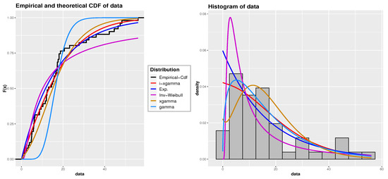
Figure 5. The fitted Pdf and Cdf for dataset 1: Leukemia-free survival times.

7.2. Application 2: Electrical Appliances

The second dataset pertains to the number of cycles to failure for 60 electrical appliances in a life test experiment (see [39]), as shown in Table 11.

Table 11. Failure time of 60 electrical appliances dataset.

0.014	0.034	0.059	0.061	0.069	0.080	0.123	0.142	0.165	0.210	0.381	0.464
0.479	0.556	0.574	0.839	0.917	0.969	0.991	1.064	1.088	1.091	1.174	1.270
1.275	1.355	1.397	1.477	1.578	1.649	1.702	1.893	1.932	2.001	2.161	2.292
2.326	2.337	2.628	2.785	2.811	2.886	2.993	3.122	3.248	3.715	3.790	3.857
3.912	4.100	4.106	4.116	4.315	4.510	4.580	5.267	5.299	5.583	6.065	9.701

To verify the compatibility of the data with the iXgamma distribution, we compare it with the Burr-III, log-normal, Lindley, and generalized exponential (Gen-Exp) distributions, following the same methodology as in the first application. The estimated parameters along with the GOF statistics are displayed in Table 12. Additionally, Figure 6 provides the empirical Cdf and histogram, along with the fitted Cdf and Pdf lines for the compared distributions. The results show that the iXgamma distribution provides a better fit compared to the other distributions for this particular dataset.

Table 12. GOF for electrical appliances dataset.

Pdf	Estimates (St.Er)		NLC	AIC	BIC	K-S	p-Value
Burr-XII	1.2676 (0.1539)	0.8944 (0.1309)	116.9868	237.9735	242.1622	0.1691	0.0571
Log-normal	0.1596 (0.1858)	1.4393 (0.1314)	116.5645	237.1289	241.3176	0.1654	0.0666
Lindley	0.7209 (0.0689)	—	107.2974	216.5948	218.6892	0.1017	0.5296
Gen-Exp	0.9159 (0.1501)	2.3190 (0.3954)	106.9694	217.9388	222.1275	0.0921	0.6539
iXgamma	0.8152 (0.0842)	—	106.3719	214.7438	216.8381	0.0881	0.7059

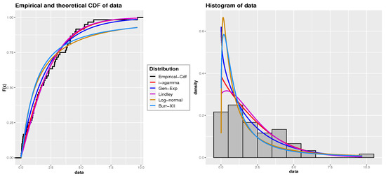
Figure 6. The fitted Pdf and Cdf for dataset 2: Electrical appliances.

7.3. Application 3: Time Between Failures

The data, sourced from [40], pertain to the time between failures for 30 repairable items, and are detailed in Table 13.

Table 13. Sorted time intervals between failures for a set of 30 repairable items.

0.11	0.30	0.40	0.45	0.59	0.63	0.70	0.71	0.74	0.77	0.94	1.06	1.17	1.18	1.23
1.23	1.24	1.46	1.49	1.74	1.82	1.86	1.97	2.23	2.37	2.46	2.63	3.46	4.36	4.73

Following a methodology similar to the first and second applications, we assess the compatibility of the iXgamma distribution both numerically and graphically with this dataset. We compare its fit with the Gamma, Rayleigh, exponential, and Xgamma distributions. The estimated parameters and GOF statistics can be found in Table 14. Figure 7 displays the empirical Cdf and histogram with the fitted Cdf and Pdf lines for the various distributions. The results suggest that the iXgamma distribution offers a better fit than the other distributions for this particular dataset.

Table 14. GOF for repairable items.

Pdf	Estimates (St.Er)		NLC	AIC	BIC	K-S	p-Value
Gamma	1.9761 (0.4733)	0.7806 (0.2126)	39.6295	83.2591	86.0615	0.2367	0.0692
Rayleigh	1.3433 (0.1226)	—	42.9182	87.8365	89.2377	0.1864	0.2479
Exponential	1.5425 (0.2815)	—	43.0053	88.0107	89.4119	0.1845	0.2588
Xgamma	1.2525 (0.1615)	—	42.6852	87.3704	88.7716	0.1745	0.3206
iXgamma	1.1396 (0.1666)	—	42.1351	86.2703	87.6715	0.1624	0.4068

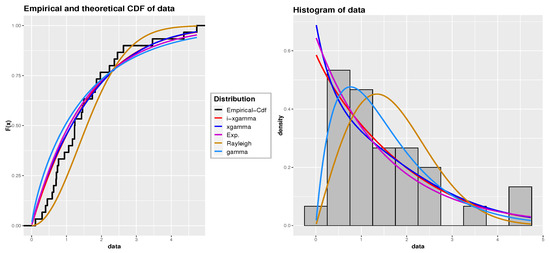
Figure 7. The fitted Pdf and Cdf for dataset 3: Time between failures dataset.

Finally, for the three given datasets, a summary of the MLE and the different Asy-CIs, including both the NA and NL methods, for the parameter $\theta$ is presented in Table 15.

Table 15. Summary of estimation for given three datasets.

Dataset	$\widehat{\mathit{\theta }}$ (Std. Error)	Asy-CI: NA	Asy-CI: NL
Leukemia free-survival times	0.1177 (0.0132)	(0.0918, 0.1435)	(0.094, 0.1466)
Electrical appliances	0.8152 (0.0842)	(0.6501, 0.9802)	(0.6658, 0.9981)
Time between failures	1.1396 (0.1666)	(0.8130, 1.4661)	(0.8556, 1.5177)

After confirming the compatibility of the previous three applications with the iXgamma distribution, our goal is to implement the PCT-II methodology using various removal schemes and estimate the distribution parameter $\theta$ using assumed estimation methods. Specifically, for Non-BE methods, we employ MLE and MPS. For BE methods, we apply various loss functions, such as SEL, LINEX at $c=1.5$, and GEL at $p=-0.5$ under TK, along with MCMC using the MH algorithm. Both point estimates and interval estimates have been calculated, with the results shown in Table 16 and Table 17, respectively. It is noteworthy that the entire dataset has been used, and these estimates are provided for comparison with those obtained under the PCT-II schemes.

Table 16. Point estimates for Non-BE and BE methods for the three datasets under various PCT-II schemes.

CS	Non-BE		BE: TK			BE: MCMC
	MLE (St.Er)	MPS	SEL	LINEX	GEL	SEL (St.Er)	LINEX	GEL
Dataset 1: Leukemia free-survival times
$\left(20,0^{*30}\right)$	0.1163 (0.0168)	0.1191	0.1142	0.1116	0.1136	0.1158 (0.0172)	0.1151	0.1156
$\left(10,0^{*29},10\right)$	0.0639 (0.0094)	0.0637	0.0627	0.0609	0.0624	0.0635 (0.0096)	0.0632	0.0635
$\left(0^{*30},10\right)$	0.0451 (0.0067)	0.0449	0.0445	0.0435	0.0443	0.0452 (0.0069)	0.0449	0.0452
Complete	0.1177 (0.0132)	0.1146	0.1163	0.1151	0.1159	0.1172 (0.0137)	0.1168	0.1170
Dataset 2: Electrical appliances
$\left(30,0^{*29}\right)$	0.8645 (0.1261)	0.8834	0.8480	0.8180	0.8435	0.8659 (0.1275)	0.8613	0.8540
$\left(15,0^{*28},15\right)$	0.3934 (0.0584)	0.3893	0.3862	0.3750	0.3841	0.3931 (0.0591)	0.3909	0.3905
$\left(0^{*29},30\right)$	0.2663 (0.0403)	0.2615	0.2613	0.2539	0.2598	0.2664 (0.0410)	0.2648	0.2651
Complete	0.8153 (0.0842)	0.8390	0.8074	0.7937	0.8052	0.8129 (0.0854)	0.8106	0.8074
Dataset 3: Time between failures
$\left(10,0^{*19}\right)$	1.2234 (0.2185)	1.1321	1.1890	1.1167	1.1793	1.2137 (0.2265)	1.2031	1.1766
$\left(5,0^{*18},5\right)$	0.8261 (0.1481)	1.0021	0.8035	0.7617	0.7966	0.8204 (0.1522)	0.8133	0.8034
$\left(0^{*19},10\right)$	0.6339 (0.1144)	0.9754	0.6171	0.5869	0.6118	0.6311 (0.1182)	0.6256	0.6209
Complete	1.1396 (0.1666)	1.2147	1.1178	1.0737	1.1113	1.1385 (0.1704)	1.1321	1.1171

Table 17. Interval estimates for the three datasets under various PCT-II schemes.

Dataset	CS	NA-CI	NL-CI	HPD-CI
Leukemia free-survival times	$\left(20,0^{*30}\right)$	(0.0833, 0.1492)	(0.1055, 0.1281)	(0.0831, 0.1502)
	$\left(10,0^{*29},10\right)$	(0.0454, 0.0824)	(0.0594, 0.0688)	(0.0452, 0.0832)
	$\left(0^{*30},10\right)$	(0.0318, 0.0583)	(0.0423, 0.0480)	(0.0319, 0.0587)
	Complete	(0.0917, 0.1437)	(0.1091, 0.1270)	(0.0906, 0.1445)
Electrical appliances	$\left(30,0^{*29}\right)$	(0.6172, 1.1118)	(0.6626, 1.1280)	(0.6271, 1.1279)
	$\left(15,0^{*28},15\right)$	(0.2788, 0.5080)	(0.3277, 0.4723)	(0.2820, 0.5145)
	$\left(0^{*29},30\right)$	(0.1872, 0.3454)	(0.2284, 0.3104)	(0.1887, 0.3505)
	Complete	(0.6502, 0.9804)	(0.6790, 0.9788)	(0.6464, 0.9853)
Time between failures	$\left(10,0^{*19}\right)$	(0.7951, 1.6517)	(0.8306, 1.8019)	(0.7984, 1.6836)
	$\left(5,0^{*18},5\right)$	(0.5358, 1.1164)	(0.6003, 1.1370)	(0.5240, 1.1214)
	$\left(0^{*19},10\right)$	(0.4096, 0.8582)	(0.4783, 0.8402)	(0.3935, 0.8551)
	Complete	(0.8131, 1.4661)	(0.8393, 1.5474)	(0.8107, 1.4743)

Figure 8, Figure 9 and Figure 10 illustrate the convergence of the MCMC estimates using the MH algorithm for the three datasets under the initial PCT-II scheme. These figures present trace plots, histograms, and cumulative means of the estimated parameter $\theta$, based on non-informative priors. These visual representations highlight the distribution of the posterior samples obtained when using informative priors for both parameters.

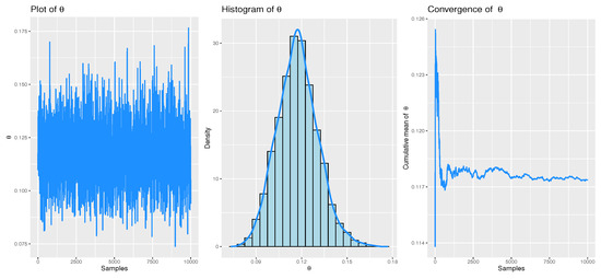
Figure 8. Convergence of MCMC for real dataset 1: Leukemia free-survival times.

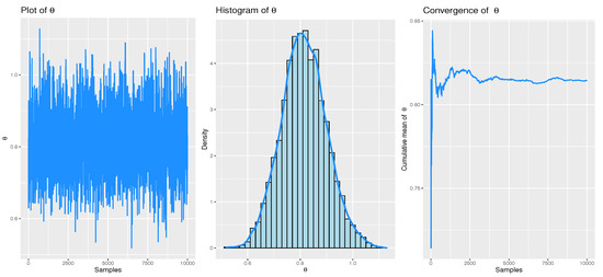
Figure 9. Convergence of MCMC for real dataset 2: Electrical appliances.

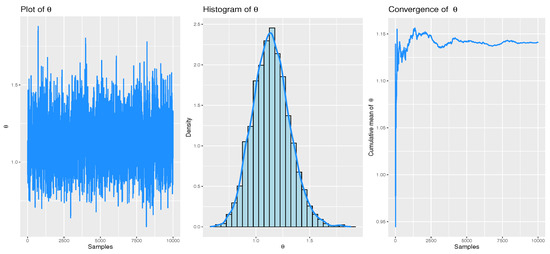
Figure 10. Convergence of MCMC for real dataset 3: Time between failures.

8. Prediction

This section addresses the issue of point prediction. Recall that under the PCT-II scheme, a number $R_j$ of live units are randomly removed from the experiment at the time of the $j\mathrm{th}$ failure, denoted as $x_{\left(j\right)}$. Let $y_{\left(jk\right)}$ represent the lifespans of these units, where $k=1,2,\cdots ,R_j$, and $j=1,2,\cdots ,m$. It is then important to note that the conditional density of $y_{\left(jk\right)}$, given the PCT-II sample x and R, provided in references [11,41], can be written as:

$$\begin{array}{ccc}\hfill f\left(y_{\left(jk\right)}\right|\mathbf{x},\theta )& =& {\displaystyle \frac{k\left(\genfrac{}{}{0pt}{}{R_j}{k}\right){\left[F\left(y_{\left(jk\right)}\right)-F\left(x_{\left(j\right)}\right)\right]}^{k-1}{(1-F\left(y_{\left(jk\right)}\right))}^{R_j-k}f\left(y_{\left(jk\right)}\right)}{{\left[1-F\left(x_j\right)\right]}^{R_j}}},y_{\left(jk\right)}>x_{\left(j\right)},\hfill \end{array}$$

where,

$$F\left(y_{\left(jk\right)}\right)=1-\left[1+{\displaystyle \frac{\theta }{\theta +3}}\left(2y_{\left(jk\right)}+{\displaystyle \frac{\theta y_{\left(jk\right)}^2}{2}}\right)\right]e^{-\theta y_{\left(jk\right)}},$$

$$F\left(x_{\left(j\right)}\right)=1-\left[1+{\displaystyle \frac{\theta }{\theta +3}}\left(2x_{\left(j\right)}+{\displaystyle \frac{\theta x_{\left(j\right)}^2}{2}}\right)\right]e^{-\theta x_{\left(j\right)}},$$

and

$$f\left(y_{\left(jk\right)}\right)={\displaystyle \frac{\theta }{3+\theta }}\left(1+\theta +\theta y_{\left(jk\right)}+{\displaystyle \frac{{\theta }^2{y}_{\left(jk\right)}^2}{2}}\right)e^{-\theta y_{\left(jk\right)}}.$$

Now, the aim is to predict the value of $y_{\left(jk\right)}$ by several prediction methods after entering all the values.

8.1. Maximum Likelihood Predictor

Here, we have to estimate and predict the value of $y_{\left(jk\right)}$; the predictive likelihood can be written as

$$\begin{array}{c}\hfill L_1\left(y_{\left(jk\right)}\right|\theta ,x)=f\left(y_{\left(jk\right)}\right|\mathbf{x},\theta )L\left(\theta \right|x).\end{array}$$

By applying the predictive log-likelihood function, $l_1=ln{L}_1\left(y_{\left(jk\right)}\right|\theta ,x)$, and computing the partial derivatives concerning both $\theta$ and $y_{\left(jk\right)}$, we derive the following expression:

$$\begin{array}{c}\hfill {\displaystyle \frac{d{L}_1}{d{y}_{\left(jk\right)}}}={\displaystyle \frac{(k-1)f\left(y_{\left(jk\right)}\right)}{F\left(y_{\left(jk\right)}\right)-F\left(x_j\right)}}-{\displaystyle \frac{(R_j-k)f\left(y_{\left(jk\right)}\right)}{1-F\left(y_{\left(jk\right)}\right)}}+{\displaystyle \frac{f^{\prime }\left(y_{\left(jk\right)}\right)}{f\left(y_{\left(jk\right)}\right)}}=0\end{array}$$

$$\begin{array}{c}{\displaystyle \frac{d{L}_1}{d\theta }}={\displaystyle \frac{n}{\theta }}-{\displaystyle \frac{n}{3+\theta }}-n\overline{x}+\sum _{i=1}^n\left({\displaystyle \frac{1+x_i+\theta x_i^2}{1+\theta +\theta x_i+{\displaystyle \frac{{\theta }^2{x}_i^2}{2}}}}\right)+{\displaystyle \frac{(k-1)[F_{\theta }^{\prime }\left(y_{\left(jk\right)}\right)-F_{\theta }^{\prime }\left(x_j\right)]}{F_{\theta }\left(y_{\left(jk\right)}\right)-F_{\theta }\left(x_j\right)}}\hfill \\ \hfill +{\displaystyle \frac{(R_j-k)\left[F_{\theta }^{\prime }\left(y_{\left(jk\right)}\right)\right]}{1-F_{\theta }\left(y_{\left(jk\right)}\right)}}+{\displaystyle \frac{f_{\theta }^{\prime }\left(y_{\left(jk\right)}\right)}{f\left(y_{\left(jk\right)}\right)}}+{\displaystyle \frac{R_j\left[F_{\theta }^{\prime }\left(x_j\right)\right]}{1-F_{\theta }\left(x_j\right)}}=0,\end{array}$$

where $f_{\theta }^{\prime }\left(y_{jk}\right)={\displaystyle \frac{df\left(y_{jk}\right)}{d\theta }}$, $F_{\theta }^{\prime }\left(x_j\right)={\displaystyle \frac{dF\left(x_j\right)}{d\theta }}$ and $F_{\theta }^{\prime }\left(y_{jk}\right)={\displaystyle \frac{dF\left(y_{jk}\right)}{d\theta }}$. Solving the above equations, we obtain the predictive maximum likelihood estimates (PMLE) of $y_{\left(jk\right)}$ and $\theta$.

8.2. Best Unbiased Predictor

Here, $y_{\left(jk\right)}$ can be predicted using the concept of the best unbiased predictor (BUP), i.e., by ${\widehat{y}}_{\left(jk\right)}$. It can also be concluded that if $E({\widehat{y}}_{\left(jk\right)}-y_{\left(jk\right)})=0$, and if $y_{\left(jk\right)}^{*}$ be any other unbiased predictor, then $Var({\widehat{y}}_{\left(jk\right)}-y_{\left(jk\right)})\le Var(y_{\left(jk\right)}^{*}-y_{\left(jk\right)})$.The BUP is given by

$$\begin{array}{ccc}\hfill {\widehat{y}}_{\left(jk\right)}& =& E\left(y_{\left(jk\right)}\right|x)\hfill \\ & =& {\int }_{x_{\left(j\right)}}^{\infty }{y}_{\left(jk\right)}f\left(y_{\left(jk\right)}\right|x,\theta )d{y}_{\left(jk\right)}.\hfill \\ & =& {\int }_{x_{\left(j\right)}}^{\infty }{y}_{\left(jk\right)}{\displaystyle \frac{k\left(\genfrac{}{}{0pt}{}{R_j}{k}\right){\left[F\left(y_{\left(jk\right)}\right)-F\left(x_{\left(j\right)}\right)\right]}^{k-1}{(1-F\left(y_{\left(jk\right)}\right))}^{R_j-k}f\left(y_{\left(jk\right)}\right)}{{\left[1-F\left(x_j\right)\right]}^{R_j}}}d{y}_{\left(jk\right)}\hfill \end{array}$$

Putting the values of $F\left(y_{\left(jk\right)}\right),F\left(x_{\left(j\right)}\right)$, and $f\left(y_{\left(jk\right)}\right)$ in the above equation, we obtain the BUP of $y_{\left(jk\right)}$.

8.3. Bayesian Predictor

In this subsection, we focus on the Bayesian predictor (BP) to forecast the $y_{\left(jk\right)}$ observations using the prior $\pi \left(\theta \right)$ along with the SEL function. The predictive posterior density, under the posterior ${\pi }^{*}\left(\theta \right)$ and prior $\pi \left(\theta \right)$, is expressed as:

$$\begin{array}{c}\hfill f^{*}\left(y_{\left(jk\right)}\right|x)={\int }_0^{\infty }f\left(y_{\left(jk\right)}\right|x,\theta ){\pi }^{*}\left(\theta \right)d\theta .\end{array}$$

Additionally, the kth observation from the $R_j$ censored units can be predicted under the SEL function as follows:

$$\begin{array}{ccc}\hfill {\widehat{y}}_{\left(jk\right)}& =& {\int }_{x_j}^{\infty }{y}_{\left(jk\right)}{f}^{*}\left(y_{\left(jk\right)}\right|x)d{y}_{\left(jk\right)}\hfill \\ & =& {\int }_0^{\infty }\left[{\int }_{x_j}^{\infty }{y}_{\left(jk\right)}f\left(y_{\left(jk\right)}\right|x,\theta )d{y}_{\left(jk\right)}\right]{\pi }^{*}\left(\theta \right)d\theta \hfill \\ & =& {\int }_0^{\infty }I\left(\theta \right){\pi }^{*}\left(\theta \right)d\theta .\hfill \end{array}$$

The above expression represents the expectation of $I\left(\theta \right)$ under the SEL function.

To obtain the desired predictive estimate, we first generate samples from the corresponding predictive posterior density using the MH algorithm. Subsequently, the predictive estimate can be obtained as follows:

$${\widehat{y}}_{\left(jk\right)}={\displaystyle \frac{1}{M-l_B}}\sum _{i=l_B}^{M}I\left({\theta }^{\left(i\right)}\right),$$

where M is the number of MCMC iterations and $l_B$ is the burn in samples.

Application to Real Datasets

In this section, we apply the prediction methods discussed earlier to the datasets introduced in Section 7, utilizing the PCT-II methodology. The first four censored observations are predicted using the proposed methods: PMLE, BUP, and BP. The predictive values for all observations are provided in Table 18. Additionally, the true observations for the considered datasets are also included in Table 18. It can be seen that the predictive estimates obtained using BP are closer to the true observations compared to those generated by the other methods.

Table 18. Estimates from different predictive methods: PMLE, BUP, and BP for ${\widehat{y}}_{\left(jk\right)}$.

Dataset	CS	J	k	True Value	PMLE ($\widehat{\mathit{\theta }}$)	${\widehat{\mathit{y}}}_{\left(\mathbf{jk}\right)}$
						PMLE	BUP	BP
Leukemia free-survival times	$\left(0^{*44},15\right)$	45	1	42.237	0.0795	42.1964	37.1302	40.9056
			2	44.638	0.0786	44.6040	38.4135	43.5464
			3	46.800	0.0784	46.4509	39.7819	45.3746
			4	47.467	0.0793	47.4428	41.2503	47.1601
Electrical appliances	$\left(0^{*19},10\right)$	20	1	1.820	—	—	1.8982	—
			2	1.860	1.0930	1.9024	2.0711	1.8852
			3	1.970	1.0922	2.0813	2.2621	2.0434
			4	2.230	1.0915	2.2806	2.4763	2.2331
Time between failures	$\left(0^{*44},15\right)$	45	1	3.715	0.7937	—	3.3807	3.4974
			2	3.790	0.8082	3.3839	3.5215	3.3516
			3	3.857	0.8080	3.5289	3.6717	3.4592
			4	3.912	0.8078	3.6837	3.8328	3.5768

9. Concluding Remarks

In this research, a new life distribution, named the iXgamma distribution, has been proposed and studied based on induced distributions. The PCT-II scheme is implemented for the proposed distribution. Several mathematical properties of the iXgamma distribution, including its reliability properties, moments, order statistics, and stress-strength reliability, have been derived. Various Non-BE methods, such as MLE and MPS, have been explored. Additionally, Bayesian procedures have been examined using numerical techniques (MCMC with the MH algorithm) and approximation methods, such as the Tierney–Kadane method based on the loss functions SEL, LINEX, and GEL. Interval estimation is also studied for MLE and BE, using Asy-CI and HPD intervals, respectively. The effectiveness of the proposed distribution is demonstrated through the analysis of three actual lifetime datasets. Our proposed distribution is shown to be superior to the Gamma, Rayleigh, exponential, and Xgamma distributions. Furthermore, Monte Carlo simulation studies were conducted to assess the performance of both non-Bayesian and BEs using the PCT-II scheme for the iXgamma distribution. Among the point estimation methods, MLE performed well in non-BE, while the Terry–Kande method excelled in BE. The HPD interval estimation method proved to be the most efficient among different interval estimation techniques. After our study, several predictor functions for the iXgamma distribution under the PCT-II scheme were derived, including the maximum likelihood predictor, best-unbiased predictor, and Bayesian predictor. Future work can explore extending the study to acceptance sampling plans, investigating informative and non-informative priors in BE, and studying causes of failure.

References

- Balakrishnan, N.; Aggarwala, R. Progressive Censoring: Theory, Methods, and Applications; Springer Science & Business Media: Berlin/Heidelberg, Germany, 2000. [Google Scholar]
- Balakrishnan, N.; Sandhu, R. A simple simulational algorithm for generating progressive Type-II censored samples. Am. Stat. 1995, 49, 229–230. [Google Scholar] [CrossRef]
- Maiti, K.; Kayal, S. Estimating Reliability Characteristics of the Log-Logistic Distribution Under Progressive Censoring with Two Applications. Ann. Data Sci. 2023, 10, 89–128. [Google Scholar] [CrossRef]
- Eryilmaz, S.; Bayramoglu, I. Spacings, exceedances, and concomitants in progressive type II censoring scheme. J. Stat. Inference 2006, 136, 527–536. [Google Scholar]
- Maiti, K.; Kayal, S. Estimation of parameters and reliability characteristics for a generalized Rayleigh distribution under progressive type-II censored sample. Commun. Stat.-Simul. Comput. 2021, 50, 3669–3698. [Google Scholar] [CrossRef]
- Tolba, A.; Almetwally, E.; Ramadan, D. Bayesian Estimation of A One-Parameter Akshaya Distribution with Progressively Type-II Censored Data. J. Stat. Appl. Probab. 2022, 11, 565–579. [Google Scholar]
- Balakrishnan, N. Progressive censoring methodology: An appraisal. Test 2007, 16, 211–259. [Google Scholar] [CrossRef]
- Balakrishnan, N.; Cramer, E. The Art of Progressive Censoring, Applications to Reliability and Quality; Springer: New York, NY, USA, 2014. [Google Scholar]
- Saha, M.; Yadav, A. Estimation of the reliability characteristics by using classical and Bayesian methods of estimation for Xgamma distribution. Life Cycle Reliab. Saf. Eng. 2021, 10, 303–317. [Google Scholar] [CrossRef]
- Abushal, T. Parametric inference of Akash distribution for Type-II censoring with analyzing of relief times of patients. Aims Math. 2021, 6, 10789–10801. [Google Scholar] [CrossRef]
- Aggarwala, R.; Balakrishnan, N. Recurrence relations for single and product moments of progressive Type-II right censored order statistics from exponential and truncated exponential distributions. Ann. Inst. Stat. Math. 1996, 48, 757–771. [Google Scholar] [CrossRef]
- Aggarwala, R.; Balakrishnan, N. Some properties of progressively censored order statistics from arbitrary and uniform distributions with applications to inference and simulation. J. Stat. Plan. Inference 1998, 70, 35–49. [Google Scholar] [CrossRef]
- Sarhan, A.; Al-Ruzaizaa, A. Statistical inference in connection with the Weibull model using type-II progressively censored data with random scheme. Pak. J. Stat. 2010, 426, 267–279. [Google Scholar]
- Sarhan, A.; Abuammoh, A. Statistical inference using progressively type-II censored data with random scheme. Int. Math. Forum 2008, 3, 1713–1725. [Google Scholar]
- Cheng, R.; Amin, N. Estimating parameters in continuous univariate distributions with a shifted origin. J. R. Stat. Soc. Ser. B Methodol. 1983, 45, 394–403. [Google Scholar] [CrossRef]
- Sen, S.; Maiti, S.; Chandra, N. The Xgamma distribution: Statistical properties and application. J. Mod. Appl. Stat. Methods 2016, 15, 38. [Google Scholar] [CrossRef]
- Montanari, G.; Mazzanti, G.; Cacciari, M.; Fothergill, J. Optimum estimators for the Weibull distribution from censored test data. Progressively censored tests. IEEE Trans. Dielectr. Electr. Insul. 1998, 5, 157–164. [Google Scholar] [CrossRef]
- Ahmed, E. Estimation and prediction for the generalized inverted exponential distribution based on progressively first-failure-censored data with the application. J. Appl. Stat. 2017, 44, 1576–1608. [Google Scholar] [CrossRef]
- Ali Mousa, M.; Jaheen, Z. Statistical Inference for the Burr Model Based on Progressively Censored Data. Comput. Math. Appl. 2002, 43, 1441–1449. [Google Scholar] [CrossRef]
- Balakrishnan, N.; Kannan, N. Point and interval estimation for parameters of the logistic distribution based on progressively Type-II censored samples. Adv. Reliab. 2001, 20, 431–456. [Google Scholar]
- Balakrishnan, N.; Sandhu, R. Best linear unbiased and maximum likelihood estimation for exponential distributions under general progressive Type-II censored samples. Indian J. Stat. Ser. B 1996, 58, 1–9. [Google Scholar]
- Alsadat, N.; Ramadan, D.; Almetwally, E.; Tolba, A. Estimation of some lifetime parameter of the unit half logistic-geometry distribution under progressively type-II censored data. J. Radiat. Res. Appl. Sci. 2023, 16, 100674. [Google Scholar] [CrossRef]
- Klein, J.; Moeschberger, M. Survival Analysis: Techniques for Censored and Truncated Data; Springer Science and Business Media: Berlin/Heidelberg, Germany, 1997. [Google Scholar]
- Ghitany, M.; Al-Awadhi, S. Maximum likelihood estimation of Burr XII distribution parameters under random censoring. J. Appl. Stat. 2002, 29, 955–965. [Google Scholar] [CrossRef]
- Lawless, J. Statistical Methods and Methods for Lifetime Data; John Wiley and Sons: New York, NY, USA, 1982. [Google Scholar]
- Panahi, H.; Asadi, S. On adaptive progressive hybrid censored Burr type III distribution: Application to the nanodroplet dispersion data. Qual. Technol. Quant. Manag. 2021, 18, 179–201. [Google Scholar] [CrossRef]
- Qin, X.; Yu, J.; Gui, W. Goodness-of-fit test for exponentiality based on spacings for general progressive Type-II censored data. J. Appl. Stat. 2020, 49, 599–620. [Google Scholar] [CrossRef]
- Salemi, U.; Rezaei, S.; Nadarajah, S. A-optimal and D-optimal censoring plans in progressively Type-II right censored order statistics. Stat. Pap. 2019, 60, 1349–1367. [Google Scholar] [CrossRef]
- Tse, S.; Yang, C.; Yuen, H. Statistical analysis of Weibull distributed lifetime data under type II progressive censoring with binomial removals. J. Appl. Stat. Taylor Fr. J. 2020, 27, 1033–1043. [Google Scholar] [CrossRef]
- Ali Mousa, M.; Jaheen, Z. Bayesian prediction for progressively censored data from the Burr model. Stat. Pap. 2002, 43, 587–593. [Google Scholar] [CrossRef]
- Ali Mousa, M.; Al-Sagheer, S. Bayesian Prediction for Progressively Type-II Censored Data from the Rayleigh Model. Commun. Stat. Theory Methods 2005, 34, 2353–2361. [Google Scholar] [CrossRef]
- Alotaibi, R.; Dey, S.; Elshahhat, A. Analysis of Progressively Type-II Inverted Generalized Gamma Censored Data and Its Engineering Application. CMES-Comput. Model. Eng. Sci. 2024, 141, 459–489. [Google Scholar] [CrossRef]
- Tolba, A. Bayesian and Non-Bayesian Estimation Methods for Simulating the Parameter of the Akshaya Distribution. Comput. J. Math. Stat. Sci. 2022, 1, 13–25. [Google Scholar] [CrossRef]
- Chen, M.; Shao, Q. Monte Carlo estimation of Bayesian credible and HPD intervals. J. Comput. Graph. Stat. 1999, 8, 69–92. [Google Scholar] [CrossRef]
- Meeker, W.; Escobar, L.; Pascual, F. Statistical Methods for Reliability Data; John Wiley & Sons: Hoboken, NJ, USA, 2022. [Google Scholar]
- Ramos, P.; Mota, A.; Ferreira, P.; Ramos, E.; Tomazella, V.; Louzada, F. Bayesian analysis of the inverse generalized Gamma distribution using objective priors. J. Stat. Comput. Simul. 2021, 91, 786–816. [Google Scholar] [CrossRef]
- Gelman, A.; Rubin, D. Inference from iterative simulation using multiple sequences. Stat. Sci. 1992, 7, 457–472. [Google Scholar] [CrossRef]
- Murthy, D.; Xie, M.; Jiang, R. Weibull Models; John Wiley & Sons: Hoboken, NJ, USA, 2004. [Google Scholar]
- Efron, B. The bootstrap and other resampling plans. In CBMS-NSF Regional Conference Series in Applied Mathematics; SIAM: Philadelphia, PA, USA, 1982. [Google Scholar]
- Gupta, R.; Kirmani, S. The role of weighted distributions in stochastic modeling. Commun. Stat. Theory Methods 1990, 19, 3147–3162. [Google Scholar] [CrossRef]
- Ahmed, E. Estimation of some lifetime parameters of generalized Gompertz distribution under progressively type-II censored data. Appl. Math. Model. 2015, 39, 5567–5578. [Google Scholar] [CrossRef]
Disclaimer/Publisher’s Note: The statements, opinions and data contained in all publications are solely those of the individual author(s) and contributor(s) and not of MDPI and/or the editor(s). MDPI and/or the editor(s) disclaim responsibility for any injury to people or property resulting from any ideas, methods, instructions or products referred to in the content. |
© 2025 by the authors. Licensee MDPI, Basel, Switzerland. This article is an open access article distributed under the terms and conditions of the Creative Commons Attribution (CC BY) license (https://creativecommons.org/licenses/by/4.0/).