Bézier Curves and Surfaces with the Blending (α, λ, s)-Bernstein Basis

Abstract

This study presents a generalized approach to Bézier curves and surfaces by utilizing the blending $(\alpha ,\lambda ,s)$-Bernstein basis. The $(\alpha ,\lambda ,s)$-Bernstein basis introduces shape parameters $\alpha$, $\lambda$, and s, which allow for more flexibility and control over the curve’s shape compared to the classical Bernstein basis. The paper explores the properties of these generalized curves and surfaces, demonstrating their ability to maintain essential geometric characteristics, such as convex hull containment and endpoint interpolation, while providing enhanced control over the shape. This work aims to contribute to the fields of computer-aided geometric design and related applications by offering a robust tool for curve and surface modeling.

1. Introduction

Bézier curves are a fundamental tool in computer-aided geometric design (CAGD), widely used in various applications such as automobile design, architecture, and medical imaging [1,2]. Traditionally, Bézier curves are defined using the Bernstein polynomial basis, which provides a parametric representation of the curves based on a set of control points. One challenge in using these curves is the limited ability to vary their shape without altering the control points. To address this, various generalizations of Bézier curves have been proposed, incorporating additional parameters into the basis polynomials to enhance flexibility. Paper [3] traced the history of the Bernstein basis, starting with its introduction by Sergei Natanovich Bernstein in 1912 as a constructive proof of the Weierstrass approximation theorem (which states that any continuous function can be approximated by a polynomial). This paper highlighted the many advantages of the Bernstein basis, such as its numerical stability, intuitive geometric interpretation (through control points), and efficient algorithms for evaluation, differentiation, and subdivision. So, Farouki’s paper emphasizes the enduring impact of this “simple but powerful idea” that continues to influence various fields a century after its inception.

Recent advancements in the field of geometric modeling have led to the development of new Bézier-like curves and surfaces that offer enhanced flexibility through the use of shape parameters. Ameer et al. [4] introduced generalized Bézier-like curves constructed with new Bernstein-like basis functions that include two shape parameters. These curves retain the essential geometric properties of classical Bézier curves, such as non-negativity and partition of unity, while providing additional control over the shape, making them highly suitable for various applications in CAGD and other engineering fields. One of the key contributions of this paper is the introduction of a new set of basis functions with two shape parameters. This allows for more flexibility in controlling the shape of the curves and surfaces compared to traditional Bézier curves and surfaces, which only have one shape parameter. The authors also provide a detailed analysis of the properties of these generalized Bézier-like curves and surfaces, which is essential for understanding their behavior and potential applications.

Similarly, recent work on generalized blended trigonometric Bézier (GBT-Bernstein) curves demonstrated the potential of blending trigonometric functions with shape parameters to create curves and surfaces that offer enhanced control and flexibility [5]. This approach not only preserves the foundational properties of classical Bernstein basis functions but also introduces new characteristics, such as symmetry and higher-order derivative continuity, making them ideal for complex geometric modeling tasks. These advancements underscore the ongoing evolution of Bézier curves and surfaces, emphasizing the importance of shape parameters in expanding their applicability and utility in modern geometric modeling.

The authors in [6] presented another generalization of Bézier curves and surfaces, also by incorporating shape parameters. The authors proposed a different set of basis functions that are also a generalization of the classical Bernstein basis functions. However, unlike the basis functions proposed by Ameer et al. [4], these basis functions only have one shape parameter. The authors also derived several properties of these generalized Bézier curves and surfaces. They demonstrated the effectiveness of their approach through several examples, showing how the shape parameter can be used to create a variety of different shapes.

Paper [7] explored Bézier curves and surfaces based on modified Bernstein polynomials. The authors proposed a modification to the classical Bernstein basis functions, which introduces a shape parameter. They then used these modified Bernstein polynomials to construct Bézier curves and surfaces. They demonstrated the effectiveness of their approach through several examples, showing how the shape parameter can be used to create a variety of different shapes. On the other hand, Mad Zain et al. [8] investigated the enhancement of flexibility and control in $\kappa$-curves using fractional Bézier curves. The authors explored the potential of utilizing fractional Bézier curves to improve the adaptability of $\kappa$-curves, which are known for their ability to represent conic sections precisely. By incorporating fractional calculus into the framework of $\kappa$-curves, the authors demonstrated how the resulting curves can achieve more nuanced and precise shape adjustments. This approach offers a novel perspective on integrating fractional calculus into CAGD, potentially leading to more sophisticated and adaptable curve and surface design tools.

Among the mentioned generalizations, $\alpha$-Bézier curves introduced the shape parameter $\alpha$ into the Bernstein basis, allowing for more control over the curve’s form. However, despite these advancements, there remains a need for a more comprehensive framework that integrates multiple shape parameters to provide even greater flexibility. In response to this need, this paper studies the $(\alpha ,\lambda ,s)$-Bernstein basis, a blending-type basis that incorporates three shape parameters: $\alpha$, $\lambda$, and s. This new basis enables the construction of generalized Bézier curves and surfaces, offering improved control over their shape while preserving essential geometric properties.

In the current paper, our aim is to construct Bézier curves represented by the blending-type $(\alpha ,\lambda ,s)$-Bernstein polynomial basis presented in [9]. The rest of the paper is organized as follows: In Section 2, we begin by defining the $(\alpha ,\lambda ,s)$-Bernstein polynomial basis and examining its properties, including its non-negativity, end point polarization, symmetry, and partition of unity. In Section 3, we define $(\alpha ,\lambda ,s)$-Bézier curves and surfaces based on this generalized basis. In Section 4, we explore the properties of these curves and surfaces, demonstrating their ability to maintain essential geometric characteristics while providing enhanced control over the shape. In Section 5, we summarize the contributions of this work and suggest potential avenues for future research.

2. (α, λ, s)-Bernstein Polynomial Basis

A widely utilized tool in CAGD is the classical Bézier curves defined, in terms of the Bernstein polynomial basis ${\displaystyle b_{r,s}\left(z\right)=\left(\genfrac{}{}{0pt}{}{r}{s}\right)z^s{(1-z)}^{r-s}}$ of degree r together with the control points $Q_s(x_s,y_s)$, as follows:

$$\begin{array}{c}\hfill B_r(Q;z)=\sum _{s=0}^r{Q}_s(x_s,y_s)b_{r,s}\left(z\right),\end{array}$$

(1)

where $z\in [0,1]$, $s=0,\dots ,r,$ and $b_{r,s}\left(z\right)=0$, $r<0$ or $s>r$.

The Bézier curves are used in a wide range of applications from automobile and architectural designs to medical imaging. One challenge of using a parametric representation of curves is to vary the shape of the curve while the control points remain unchanged. In this direction, one of the remarkable attempts is the rational Bézier curves which have their own deficiencies. On the one hand, when tangency properties are needed to be controlled, differentiation results in higher-order curves. On the other hand, the representation of these curves contains weights in addition to the control points. Thus, various generalizations of the Bézier curves, by presenting shape parameters in the basis polynomials, have been the subject of several papers in recent decades [10,11,12].

Among these papers, in [12], $\alpha$-Bézier curves are constructed as

$$\begin{array}{c}\hfill B_r(Q;z;\alpha )=\sum _{s=0}^r{Q}_s(x_s,y_s)b_{r,s}^{\alpha }\left(z\right),\end{array}$$

(2)

where for $\alpha \in [0,1]$, $b_{r,s}^{\alpha }\left(z\right)$ is the $\alpha$-Bernstein polynomial introduced in [13] as

$$b_{r,s}^{\alpha }\left(z\right)=\left[\left({\displaystyle \genfrac{}{}{0pt}{}{r-2}{s}}\right)(1-\alpha )z+\left({\displaystyle \genfrac{}{}{0pt}{}{r-2}{s-2}}\right)(1-\alpha )(1-z)+\left({\displaystyle \genfrac{}{}{0pt}{}{r}{s}}\right)\alpha z(1-z)\right]z^{s-1}{(1-z)}^{r-s-1}.$$

(3)

Note that this polynomial has been used in many studies to construct certain positive linear operators [14,15,16]. We begin with the $\lambda$-Bernstein polynomials which are defined for $r\ge 2$ in [17] as:

$$\begin{array}{c}\hfill a_{r,i}^{\lambda }\left(z\right)=\left\{\begin{array}{cc}{b}_{r,0}\left(z\right)-{\displaystyle \frac{\lambda }{r+1}}{b}_{r+1,1}\left(z\right),\hfill & i=0,\hfill \\ \\ b_{r,i}\left(z\right)+\lambda \left({\displaystyle \frac{r-2i+1}{r^2-1}}\right)b_{r+1,i}\left(z\right)-\lambda \left({\displaystyle \frac{r-2i-1}{r^2-1}}\right)b_{r+1,i+1}\left(z\right),\hfill & 1\le i\le r-1,\hfill \\ \\ b_{r,r}\left(z\right)-{\displaystyle \frac{\lambda }{r+1}}{b}_{r+1,r}\left(z\right),\hfill & i=r\hfill \end{array}\right.\end{array}$$

(4)

and when $r=0,1$, we make a convenience of the following:

$$\begin{array}{cc}\hfill a_{0,0}^{\lambda }\left(z\right)& =b_{0,0}\left(z\right)=1,\hfill \\ \hfill a_{1,0}^{\lambda }\left(z\right)& =b_{1,0}\left(z\right)=1-z,a_{1,1}^{\lambda }\left(z\right)=b_{1,1}\left(z\right)=z.\hfill \end{array}$$

(5)

The $\lambda$-Bernstein polynomials are used to construct some approximating operators in the literature [18,19,20,21,22,23,24].

By means of $\lambda$- and $\alpha$-Bernstein polynomials, in [9], $(\alpha ,\lambda ,s)$-Bernstein polynomials are defined as:

$$\begin{array}{c}\hfill q_{r,i}^{\alpha ,\lambda ,s}\left(z\right)=\left\{\begin{array}{cc}{a}_{r,i}^{\lambda }\left(z\right),\hfill & r<s,\hfill \\ \\ (1-\alpha )[z{a}_{r-s,i-s}^{\lambda }\left(z\right)+(1-z)a_{r-s,i}^{\lambda }\left(z\right)]+\alpha a_{r,i}^{\lambda }\left(z\right),\hfill & r\ge s,\hfill \end{array}\right.\end{array}$$

(6)

where $z,\alpha \in [0,1]$, $\lambda \in [-1,1]$, s is a positive integer, and $b_{r,s}\left(z\right)$ is the classical Bernstein basis functions. We refer the reader to studies [16,25] on certain kinds of $(\alpha ,\lambda )$-Bernstein-type operators, their extensions or modifications, and their approximation properties. We also refer the reader to some recent important approximation theory studies on the effect of shape parameters in approximating operators [15,26,27].

Remark 1.

Note that

• The λ-Bernstein polynomial basis reduces to the classical Bernstein polynomial basis when $\lambda =0$.
• The $(\alpha ,\lambda ,s)$-Bernstein polynomial basis reduces to the λ-Bernstein polynomial basis when $\alpha =1$ or, by Lemma 2 below, $s=1$.
• The $(\alpha ,\lambda ,s)$-Bernstein polynomial basis reduces to the classical Bernstein polynomial basis when $\lambda =0$ and $\alpha =1$ or $\lambda =0$ and $s=1$.

In [17,28], for $z\in [0,1]$ and $\lambda \in [-1,1]$, the following properties of $\lambda$-Bernstein polynomials are obtained:

• $a_{r,i}^{\lambda }\left(z\right)$ is non-negative.
• End Point Polarization:

  $$\begin{array}{c}\hfill a_{r,i}^{\lambda }\left(0\right)=\left\{\begin{array}{cc}0,\hfill & i\ne 0\hfill \\ \\ 1,\hfill & i=0\hfill \end{array}\right.,a_{r,i}^{\lambda }\left(1\right)=\left\{\begin{array}{cc}0,\hfill & \mathit{i}\ne r\hfill \\ \\ 1,\hfill & \mathit{i}=r.\hfill \end{array}\right.\end{array}$$

  (7)
• Symmetry:

  $$\begin{array}{c}\hfill a_{r,i}^{\lambda }\left(z\right)=a_{r,r-i}^{\lambda }(1-z).\end{array}$$

  (8)
• Partition of Unity: ${\displaystyle \sum _{i=0}^r{a}_{r,i}^{\lambda }\left(z\right)=1.}$

Lemma 1.

For $z,\alpha \in [0,1]$, $\lambda \in [-1,1]$ and any positive integer s,

$\left(1\right)$

$q_{r,i}^{\alpha ,\lambda ,s}\left(z\right)$ is non-negative.

$\left(2\right)$

End Point Polarization:

$$\begin{array}{c}\hfill q_{r,i}^{\alpha ,\lambda ,s}\left(0\right)=\left\{\begin{array}{cc}0,\hfill & i\ne 0\hfill \\ 1,\hfill & i=0\hfill \end{array}\right.,q_{r,i}^{\alpha ,\lambda ,s}\left(1\right)=\left\{\begin{array}{cc}0,\hfill & \mathit{i}\ne r\hfill \\ 1,\hfill & \mathit{i}=r.\hfill \end{array}\right.\end{array}$$

(9)

$\left(3\right)$

Symmetry:

$$\begin{array}{c}\hfill q_{r,i}^{\alpha ,\lambda ,s}\left(z\right)=q_{r,r-i}^{\alpha ,\lambda ,s}(1-z).\end{array}$$

(10)

$\left(4\right)$

Partition of Unity: ${\displaystyle \sum _{i=0}^r{q}_{r,i}^{\alpha ,\lambda ,s}\left(z\right)=1.}$

Proof. 

Each property can be obtained by direct calculations using the above (1)–(4) properties of the $\lambda$-Bernstein polynomials. □

Figure 1 demonstrates the impact of fixing two parameters and varying the third, revealing the enhanced flexibility of the ($\alpha ,\lambda ,s$)-Bernstein basis in controlling curve shapes. In part (a), $\lambda (=0.5)$ and $s(=2)$ are fixed while the parameter $\alpha$ varies from $0.4$ to $0.9$; in part (b), $\alpha (=0.5)$ and $s(=2)$ are fixed while the parameter $\lambda$ varies from $-0.6$ to $0.6$, and in part (c), $\lambda (=0.5)$ and $\lambda (=0.7)$ are fixed while the parameter s varies from 2 to 4. It can obviously be seen that the ($\alpha ,\lambda ,s$)-Bernstein basis preserves the geometric feature of the classical Bernstein basis.

Lemma 2.

For any $\lambda \in [-1,1]$, each r-th degree λ-Bernstein polynomial can be decomposed as:

$$\begin{array}{c}\hfill a_{r,i}^{\lambda }\left(z\right)=(1-z)a_{r-1,i}^{\lambda }\left(z\right)+z{a}_{r-1,i-1}^{\lambda }\left(z\right).\end{array}$$

(11)

Proof. 

We substitute the well-known recursive formula of classical Bernstein polynomials

$$b_{r,i}\left(z\right)=(1-z)b_{r-1,i}\left(z\right)+z{b}_{r-1,i-1}\left(z\right)$$

into the definition of $\lambda$-Bernstein polynomials given in (4) and obtain:

$$\begin{array}{cc}\hfill a_{r,i}^{\lambda }\left(z\right)& =(1-z)b_{r-1,i}\left(z\right)+z{b}_{r-1,i-1}\left(z\right)+\lambda \left({\displaystyle \frac{r-2i+1}{r^2-1}}\right)\left[(1-z)b_{r,i}\left(z\right)+z{b}_{r,i-1}\left(z\right)\right]\hfill \\ \hfill & -\lambda \left({\displaystyle \frac{r-2i-1}{r^2-1}}\right)\left[(1-z)b_{r,i+1}\left(z\right)+z{b}_{r,i}\left(z\right)\right]\hfill \\ \hfill & =(1-z)\left[b_{r-1,i}\left(z\right)+\lambda \left({\displaystyle \frac{r-2i+1}{r^2-1}}\right)b_{r,i}\left(z\right)-\lambda \left({\displaystyle \frac{r-2i-1}{r^2-1}}\right)b_{r,i+1}\left(z\right)\right]\hfill \\ \hfill & +z\left[b_{r-1,i-1}\left(z\right)+\lambda \left({\displaystyle \frac{r-2i+1}{r^2-1}}\right)b_{r,i-1}\left(z\right)-\lambda \left({\displaystyle \frac{r-2i-1}{r^2-1}}\right)b_{r,i}\left(z\right)\right]\hfill \\ \hfill & =(1-z)a_{r-1,i}^{\lambda }\left(z\right)+z{a}_{r-1,i-1}^{\lambda }\left(z\right).\hfill \end{array}$$

□

Lemma 3 is the $(\alpha ,\lambda ,s)$-Bernstein polynomial basis analogue of Lemma 2:

Lemma 3.

For any $\alpha \in [0,1]$, $\lambda \in [-1,1]$, and any positive integer s, each r-th degree $(\alpha ,\lambda ,s)$-Bernstein polynomial can be decomposed as:

$$\begin{array}{c}\hfill q_{r,i}^{\alpha ,\lambda ,s}\left(z\right)=(1-z)q_{r-1,i}^{\alpha ,\lambda ,s}\left(z\right)+z{q}_{r-1,i-1}^{\alpha ,\lambda ,s}\left(z\right).\end{array}$$

(12)

Proof. 

Let $r\ge s$. If we substitute (11) into (6), we obtain:

$$\begin{array}{cc}\hfill q_{r,i}^{\alpha ,\lambda ,s}\left(z\right)& =(1-\alpha )[z\left((1-z)a_{r-s-1,i-s}^{\lambda }\left(z\right)+z{a}_{r-s-1,i-s-1}^{\lambda }\left(z\right)\right)\hfill \\ \hfill & +(1-z)\left((1-z)a_{r-s-1,i}^{\lambda }\left(z\right)+z{a}_{r-s-1,i-1}^{\lambda }\left(z\right)\right)]\hfill \\ \hfill & +\alpha \left[(1-z)a_{r-1,i}^{\lambda }\left(z\right)+z{a}_{r-1,i-1}^{\lambda }\left(z\right)\right]\hfill \\ \hfill & =(1-z)\left[(1-\alpha )\left(z{a}_{r-s-1,i-s}^{\lambda }\left(z\right)+(1-z)a_{r-s-1,i}^{\lambda }\left(z\right)\right)+\alpha a_{r-1,i}^{\lambda }\left(z\right)\right]\hfill \\ \hfill & +z\left[(1-\alpha )\left(z{a}_{r-s-1,i-s-1}^{\lambda }\left(z\right)+(1-z)a_{r-s-1,i-1}^{\lambda }\left(z\right)\right)+\alpha a_{r-1,i-1}^{\lambda }\left(z\right)\right]\hfill \\ \hfill & =(1-z)q_{r-1,i}^{\alpha ,\lambda ,s}\left(z\right)+z{q}_{r-1,i-1}^{\alpha ,\lambda ,s}\left(z\right).\hfill \end{array}$$

□

Remark 2.

It is shown in [28] that when $r\ge 2$, the λ-Bernstein polynomials have the following end point derivatives:

$$\begin{array}{c}\hfill {\displaystyle \frac{d}{dz}}{a}_{r,i}^{\lambda }\left(0\right)=\left\{\begin{array}{cc}-(r+\lambda ),\hfill & i=0\hfill \\ (r+\lambda ),\hfill & i=1\hfill \\ 0,\hfill & 2\le i\le r\hfill \\ \hfill \end{array}\right.,{\displaystyle \frac{d}{dz}}{a}_{r,i}^{\lambda }\left(1\right)=\left\{\begin{array}{cc}0,\hfill & 0\le i<r-1\hfill \\ -(r+\lambda ),\hfill & i=r-1\hfill \\ (r+\lambda ),\hfill & i=r.\hfill \end{array}\right.\end{array}$$

(13)

Theorem 1.

Let s be a positive integer, $r\ge 2,$ and $r\ge s$; then, the $(\alpha ,\lambda ,s)$-Bernstein polynomials have the following end point derivatives

(a) for the case $r-s\ge 2$,

$$\begin{array}{c}\hfill {\displaystyle \frac{d{q}_{r,i}^{\alpha ,\lambda ,s}}{dz}}\left(0\right)=\left\{\begin{array}{cc}(1-\alpha )(s-1)-(r+\lambda ),\hfill & i=0,\hfill \\ r+\lambda ,\hfill & i=s=1\hfill \\ (r+\lambda )-s(1-\alpha ),\hfill & i=1\ne s,\hfill \\ 1-\alpha ,\hfill & 2\le i=s\hfill \\ 0,\hfill & 2\le i\le r,i\ne s,\hfill \\ \hfill \end{array}\right.\end{array}$$

(14)

$$\begin{array}{c}\hfill {\displaystyle \frac{d{q}_{r,i}^{\alpha ,\lambda ,s}}{dz}}\left(1\right)=\left\{\begin{array}{cc}0,\hfill & i=0,1\mathit{or}r-s\ne i<r-1\hfill \\ s(1-\alpha )-(r+\lambda ),\hfill & i=r-1,s\ne 1\hfill \\ -(r+\lambda ),\hfill & i=r-s,s=1\hfill \\ -(1-\alpha ),\hfill & i=r-s,s\ge 2\hfill \\ (1-s)(1-\alpha )+(r+\lambda ),\hfill & i=r,\hfill \end{array}\right.\end{array}$$

(15)

(b) for the case $r-s<2$, that is, when $r-s=0$ or $r-s=1$,

$$\begin{array}{c}\hfill {\displaystyle \frac{d{q}_{r,i}^{\alpha ,\lambda ,s}}{dz}}\left(0\right)=\left\{\begin{array}{cc}-(1-\alpha )-\alpha (r+\lambda ),\hfill & r=s,i=0,\hfill \\ \alpha (r+\lambda ),\hfill & r=s,i=1,\hfill \\ 0,\hfill & \mathit{i}\ne r=s,2\le i<r,\mathit{or}r=s+1,s\ne i\ge 2\hfill \\ 1-\alpha ,\hfill & r=i=s\mathit{or}r=s+1,s=i,2\le i\le r,\hfill \\ -2(1-\alpha )-\alpha (r+\lambda ),\hfill & r=s+1,i=0,\hfill \\ (1-\alpha )+\alpha (r+\lambda ),\hfill & r=s+1,i=1\ne s,\hfill \end{array}\right.\end{array}$$

(16)

$$\begin{array}{c}\hfill {\displaystyle \frac{d{q}_{r,i}^{\alpha ,\lambda ,s}}{dz}}\left(1\right)=\left\{\begin{array}{cc}(1-\alpha )+\alpha (r+\lambda ),\hfill & \mathit{i}=r=s\hfill \\ -(1-\alpha ),\hfill & r=s,i=0\mathit{or}r=s+1,i=1\ne s,\hfill \\ 2(1-\alpha )+\alpha (r+\lambda ),\hfill & r=s+1=i,\hfill \\ -\alpha (r+\lambda ),\hfill & r=s+1,i=s=1\mathit{or}i=r-1,r=s\ge 2\hfill \\ -(1-\alpha )-\alpha (r+\lambda ),\hfill & i=s=r-1\hfill \\ 0,\hfill & r=s+1,i=0\mathit{or}1\le i<r-1,r=s>2\mathit{or}2\le i<r-1=s,\hfill \end{array}\right.\end{array}$$

(17)

and

$$\begin{array}{c}\hfill {\displaystyle \frac{d{q}_{2,1}^{\alpha ,\lambda ,1}}{dz}}\left(1\right)=-{\displaystyle \frac{d{q}_{2,1}^{\alpha ,\lambda ,1}}{dz}}\left(0\right)=-\left[2(1-\alpha )+\alpha (r+\lambda )\right].\end{array}$$

(18)

Proof. 

First, we note the following facts:

(i)

We consider only the case $r\ge s$, $s\ge 1$ and $r\ge 2$, since by (4) and (6), the $(\alpha ,\lambda ,s)$-Bézier basis is defined for $s\ge 1$, $r\ge 2$; and $q_{r,i}^{\lambda ,\alpha ,s}\left(z\right)=a_{r,i}^{\lambda }\left(z\right)$, if $r<s$.

(ii)

Even if $r\ge s$, $s\ge 1$, we may still have that $0\le r-s<2$. For this reason, we consider two cases, $0\le r-s<2$ and $\ge 2$. Hence, whenever it is needed, we make use of (5).

(iii)

For a Bernstein-type basis, it is obvious that $0\le i\le r$. However, definition (6) for $r\ge s$ leads us to the cases where $i-s<0$ and $r-s<i$. For such cases, it is convenient to take $a_{k,j}^{\lambda }\left(z\right)=0$ whenever $\mathit{j}>k$ or $j<0$.

Now, differentiating (6), for $r\ge s$, with regard to z, we obtain

$${\displaystyle \frac{d{q}_{r,i}^{\alpha ,\lambda ,s}}{dz}}\left(z\right)=(1-\alpha )\left[a_{r-s,i-s}^{\lambda }\left(z\right)+z{\displaystyle \frac{d{a}_{r-s,i-s}^{\lambda }}{dz}}\left(z\right)-a_{r-s,i}^{\lambda }\left(z\right)+(1-z){\displaystyle \frac{d{a}_{r-s,i}^{\lambda }}{dz}}\left(z\right)\right]+\alpha {\displaystyle \frac{d{a}_{r,i}^{\lambda }}{dz}}\left(z\right).$$

(19)

(a)

To derive (14) and (15), we first substitute $z=0$ and $z=1$;, respectively, and then examine the indices in (19) considering (7) and (13). Thus, we obtain the cases indicated in Equations (14) and (15). In each case, substituting the proper values from (7) and (13) and using the facts (i)–(iii), we obtain the results for $r-s\ge 2$.

(b)

For this part, we have $r-s<2$, that is, $r-s=0$ or $r-s=1$. Hence, by similar considerations and suitable substitutions from (7) and (13) into (19), together with the facts (i)–(iii), we obtain the desired results, (16) and (17).

□

3. (α, λ, s)-Bézier Curves and Their Properties

In the sequel, we call the generalized Bézier curves defined by the $(\alpha ,\lambda ,s)$-Bernstein polynomial basis $(\alpha ,\lambda ,s)$-Bézier curves, which are given by the following formula:

$${\displaystyle C^{\alpha ,\lambda ,s}(z;\mathbf{P})=\sum _{i=0}^r{q}_{r,i}^{\alpha ,\lambda ,s}\left(z\right){\mathbf{P}}_i(x_i,y_i),}$$

(20)

where $\alpha \in [0,1]$, $\lambda \in [-1,1]$, $z\in [0,1]$, s is a positive integer, $q_{r,i}^{\alpha ,\lambda ,s}\left(z\right)$ is the $(\alpha ,\lambda ,s)$-Bézier basis in (6), and $\mathbf{P}=\{{\mathbf{P}}_i(x_i,y_i):i=0,1,...,r\}$ is the set of control points ${\mathbf{P}}_i(x_i,y_i)$ for $i=0,1,...,r.$

The $(\alpha ,\lambda ,s)$-Bézier curves given in (20) satisfy the following properties which are immediate consequences of Lemma 1:

• $C^{\alpha ,\lambda ,s}\left(z\right)$ lies in the convex hull of the set $\mathbf{P}=\{{\mathbf{P}}_i(x_i,y_i):i=0,1,...,r\}$, by Lemma 1 (1) and (4).
• By Lemma 1 (2),

  $$\begin{array}{c}\hfill C^{\alpha ,\lambda ,s}(0;\mathbf{P})={\mathbf{P}}_0(x_0,y_0),C^{\alpha ,\lambda ,s}(1;\mathbf{P})={\mathbf{P}}_r(x_r,y_r).\end{array}$$

  (21)
• By Lemma 1 (3), we conclude that reversing the order of the control points gives the same $(\alpha ,\lambda ,s)$-Bézier curve. That is, if $C^{\alpha ,\lambda ,s}(z;\mathbf{P})$ is the $(\alpha ,\lambda ,s)$-Bézier curve with the control points $\mathbf{P}=\{{\mathbf{P}}_i(x_i,y_i):i=0,1,...,r\}$ and $\mathbf{Q}=\{{\mathbf{Q}}_i(x_i,y_i)={\mathbf{P}}_{r-i}(x_{r-i},y_{r-i}):i=0,1,...,r\}$, then

  $$C^{\alpha ,\lambda ,s}(z;\mathbf{Q})=C^{\alpha ,\lambda ,s}(1-z;\mathbf{P}).$$

  (22)

In Figure 2 and Figure 3 below, one can observe that the geometric properties (convex hull, end point interpolation, and symmetry) are satisfied by the cubic ($\alpha ,\lambda ,s$)-Bezier curves having different shape parameters values. Moreover, it can be seen that changing the values of the shape parameters allows us to adjust the shape of the curve without having to manipulate the control points in a way that preserves the geometry of classical Bézier curves.

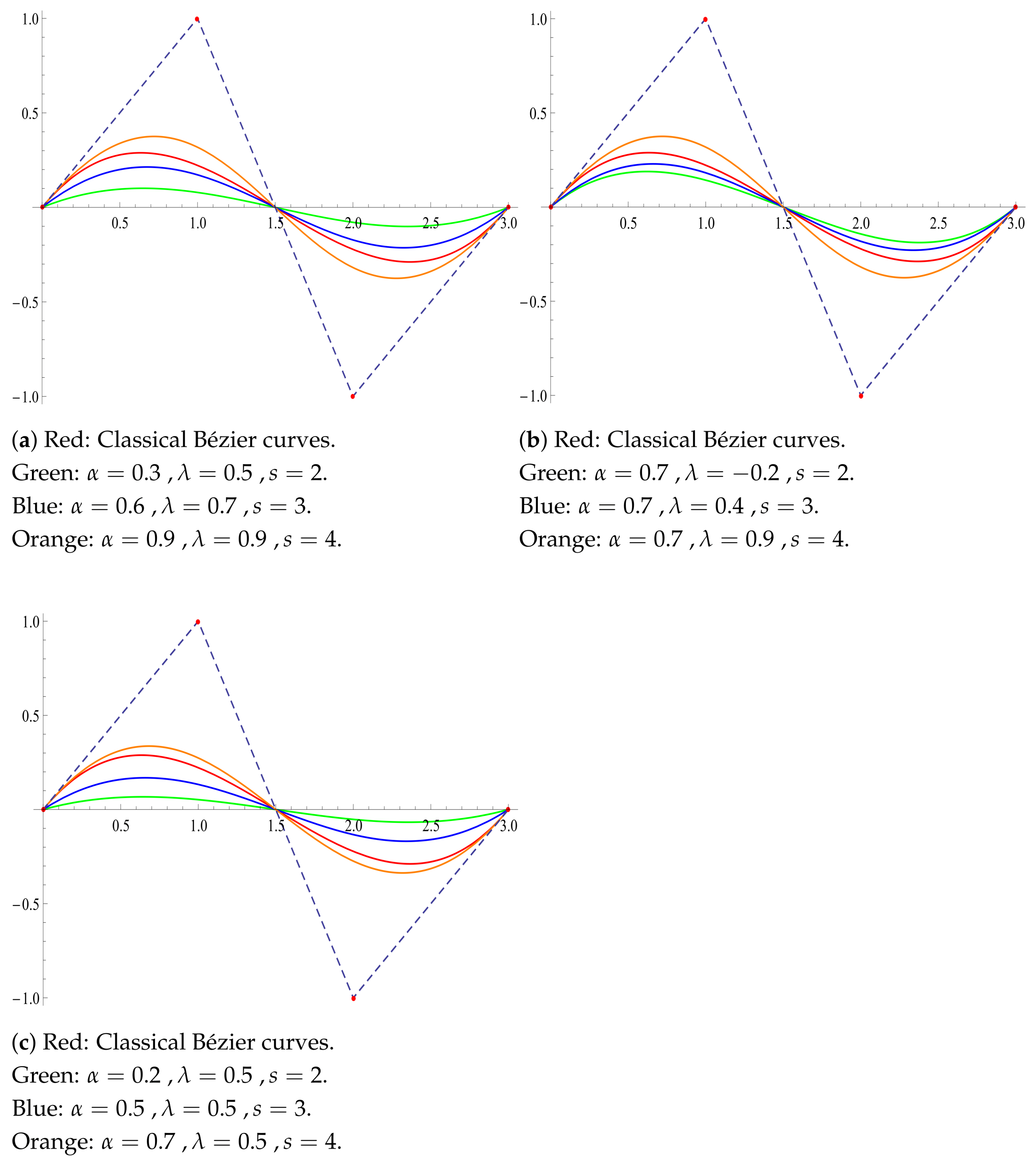
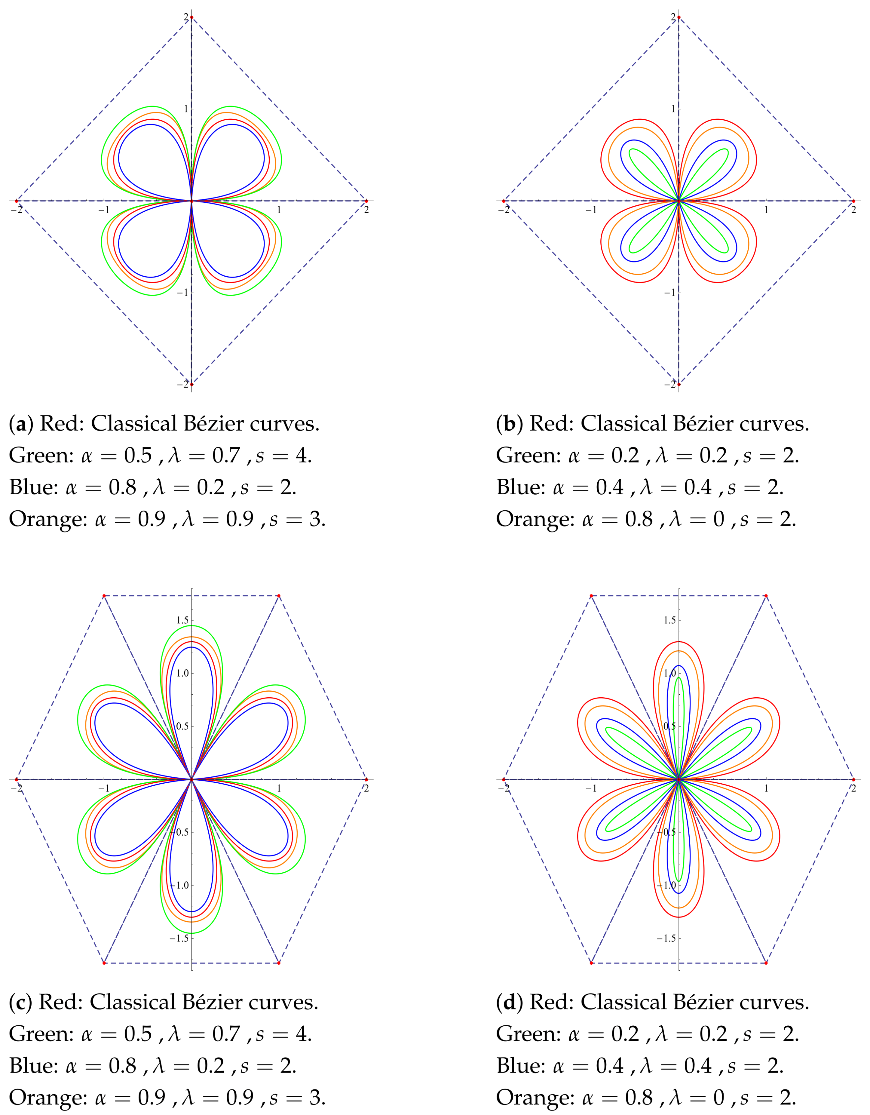
In Figure 2, we illustrate the flexibility of ($\alpha ,\lambda ,s$)-Bézier curves compared to classical-Bézier curves with a fixed set of control points ${\mathbf{P}}_0=(0,0)$, ${\mathbf{P}}_1=(1,1)$, ${\mathbf{P}}_2=(1.5,0)$, ${\mathbf{P}}_3=(2,-1)$, and ${\mathbf{P}}_4=(3,0)$. We compare the flexibility of the remaining parameter on the shape while keeping certain parameters fixed. For instance, in parts (b) and (c), the parameters $\alpha$ and $\lambda$ are fixed and the other two parameters change. In part (a), all parameters change, which enables us to compare various ($\alpha ,\lambda ,s$)-Bézier curves with the classical one.

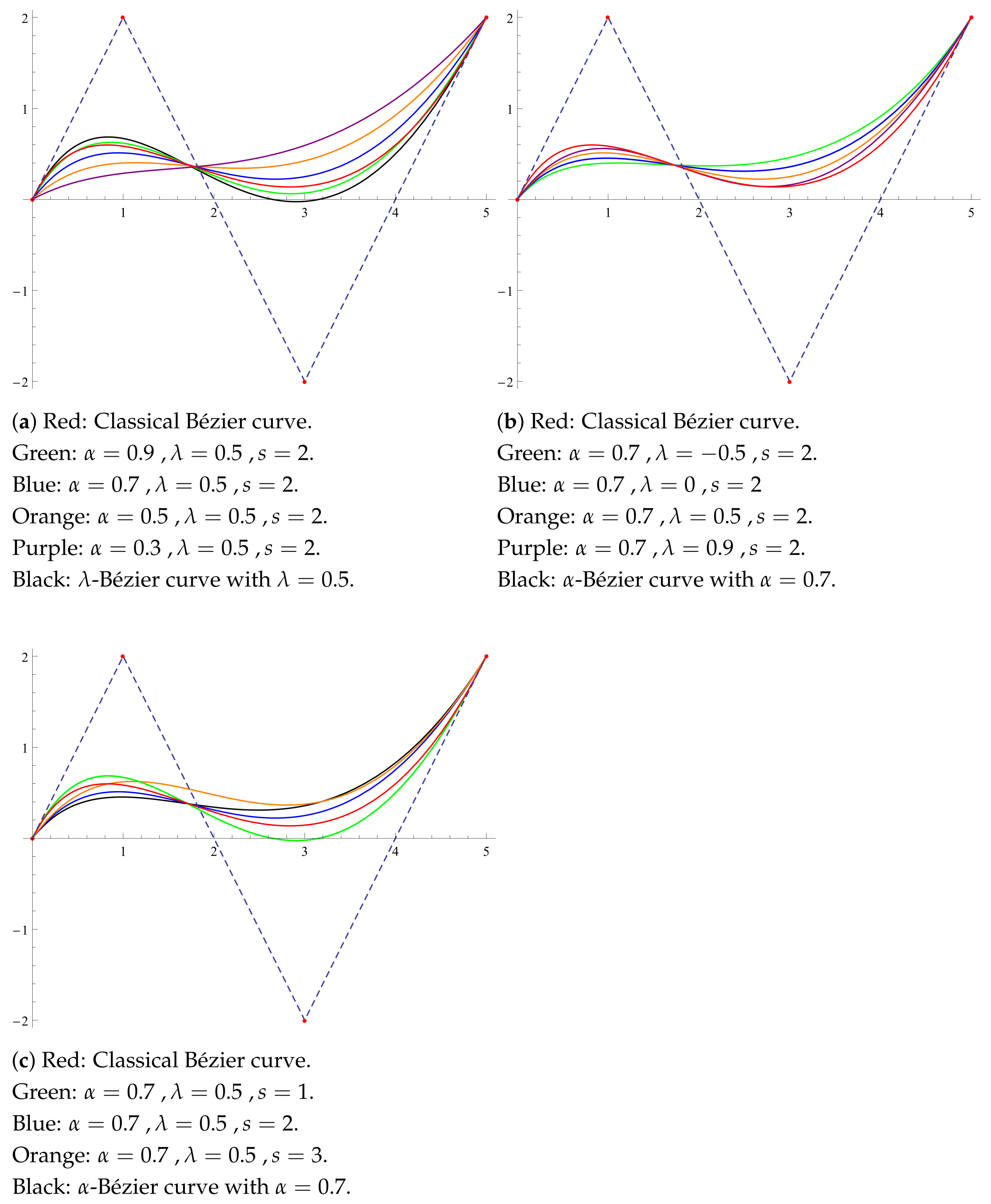
Figure 3 illustrates the envisioned flexibility of $(\alpha ,\lambda ,s)$-Bézier curves compared to (a) $\lambda$-Bézier curves ($\lambda$ and s are fixed; $\alpha$ varies), (b) $\alpha$-Bézier curves ($\alpha$ and s are fixed; $\lambda$ varies), and (c) $\lambda$- and $\alpha$-Bézier curves ($\alpha$ and $\lambda$ are fixed; s varies). In part (c), Green, taking $s=1$, by Lemma 2, the $(\alpha ,\lambda ,s)$-Bézier curve reduces to the $\lambda$-Bézier curve.

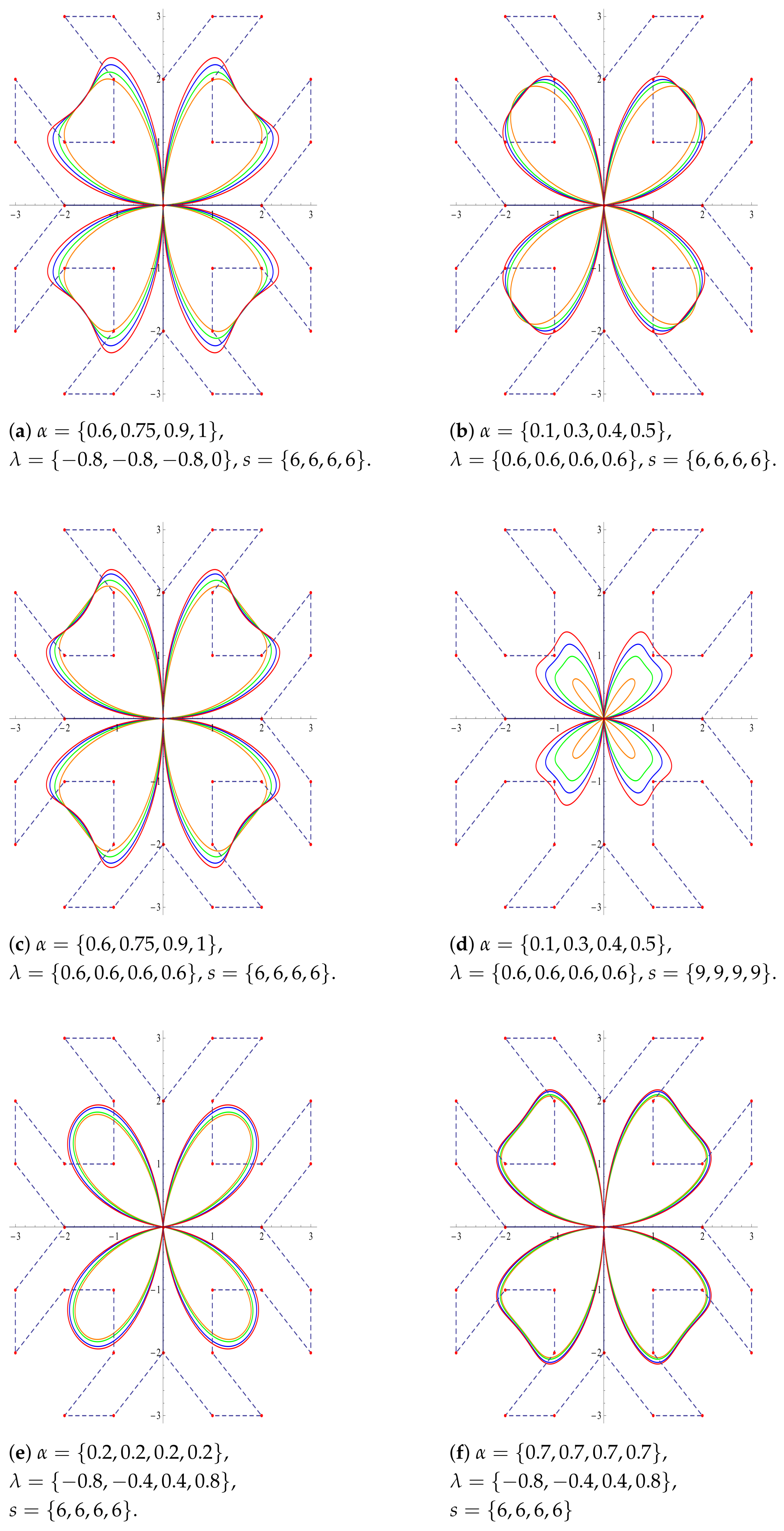
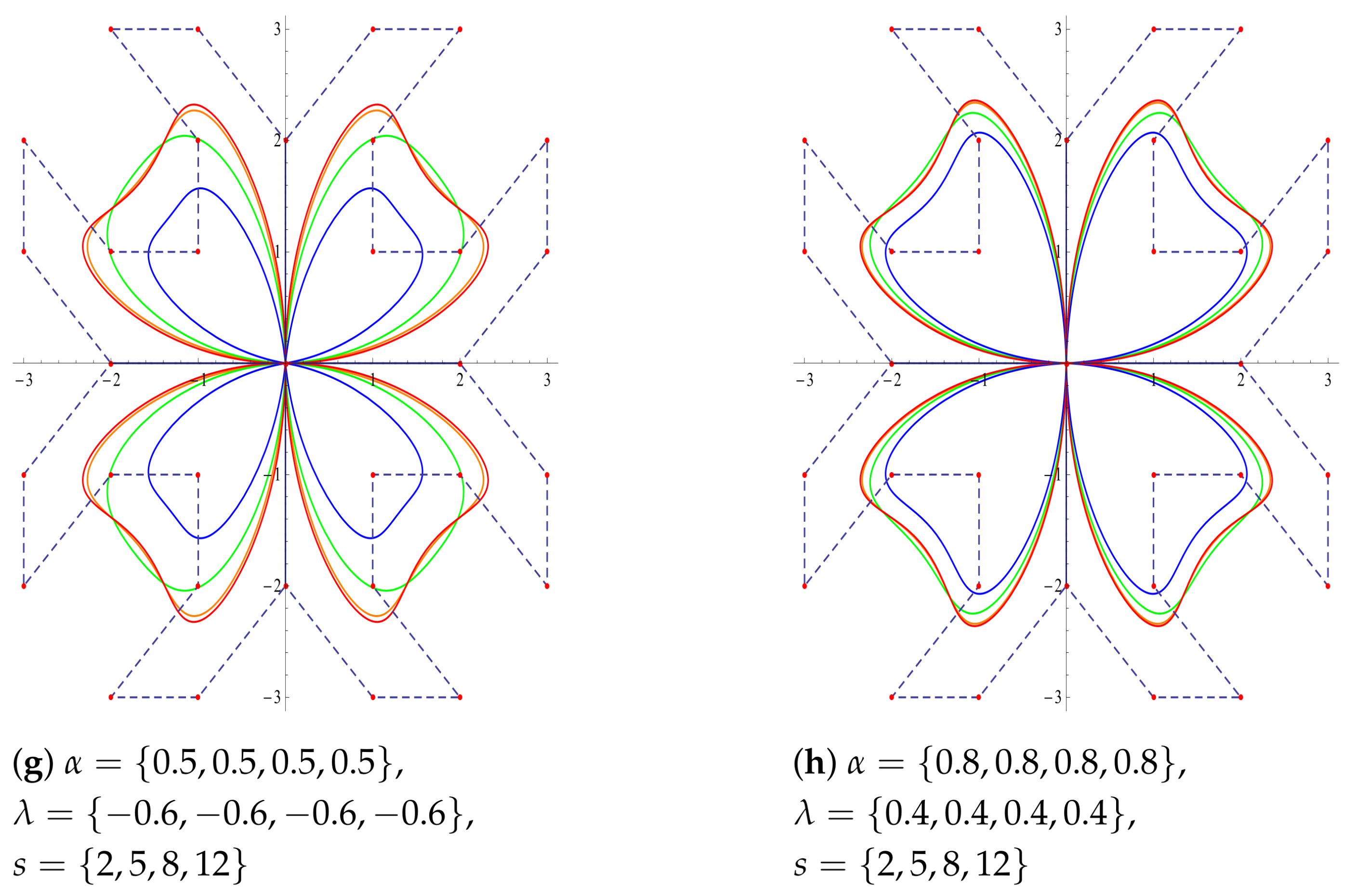
In Figure 4, we consider the graphs of leaf clovers via $(\alpha ,\lambda ,s)$-Bézier curves, with different shape parameters in each part, and the classical Bézier curve in order to compare the flexibility benefits of shape parameters over the classical one. We conduct a comparison by using the same control points in parts (a) and (b) and apply the same approach to parts (c) and (d).

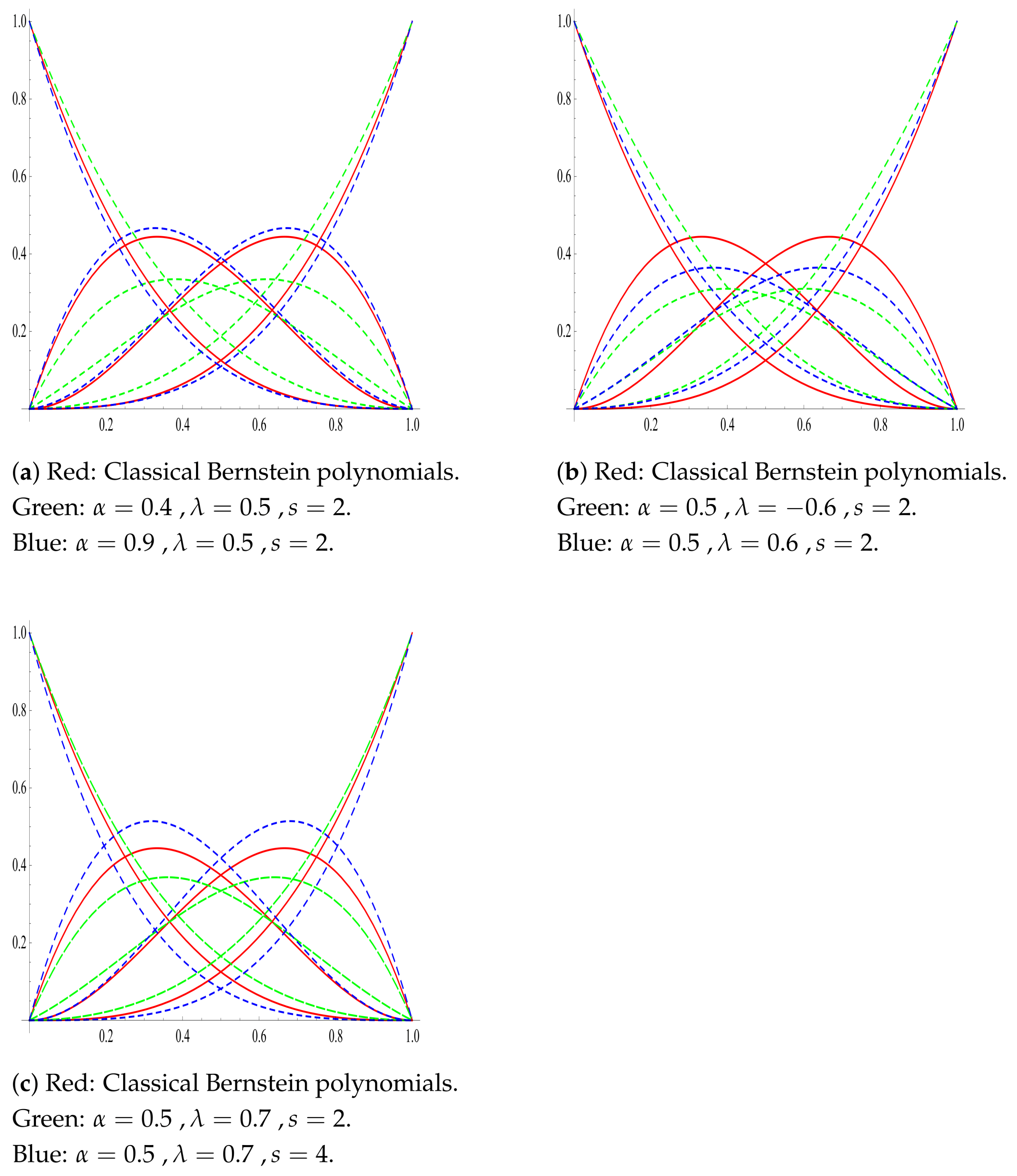
Note that in the below Figure Figure 5, Figure 6 and Figure 7, we have provided a set comprising four distinct values for each of the three parameters $\alpha ,\lambda ,s$. In each section of these figures, the $({\alpha }_i,{\lambda }_i,s_i)$-Bernstein curves are plotted based on the values in these sets, with the colors assigned as follows: $i=1$ (orange), $i=2$ (green), $i=3$ (blue), and $i=4$ (red).

In each part of Figure 5, two of the three parameters are kept constant, while the remaining parameter is varied. When different parameter values are given, a significant variety is observed in the obtained geometric shapes. The various values of the parameters are considered together with their effects on the geometry. For example, in parts (e) and (f), the parameter $\lambda$ varies among the same values and s is kept constant at the same value; on the other hand, the parameter $\alpha$ is kept constant at different values, providing a comparison of the effect of $\alpha$.

Theorem 2.

For positive s, $r\ge 2$ and $r\ge s$, the $(\alpha ,\lambda ,s)$-Bézier curves have the following end point derivative properties:

(a) If $r-s\ge 2$,

$$\begin{array}{cc}\hfill {\displaystyle \frac{d}{dz}}{C}^{\alpha ,\lambda ,s}(0;\mathit{P})=(1-\alpha )({\mathit{P}}_s-{\mathit{P}}_0)+[r+\lambda -s(1-\alpha )]({\mathit{P}}_1-{\mathit{P}}_0),& s\ge 1,\end{array}$$

(23)

and

$$\begin{array}{c}\hfill {\displaystyle \frac{d}{dz}}{C}^{\alpha ,\lambda ,s}(1;\mathit{P})=\left\{\begin{array}{cc}(r+\lambda )({\mathit{P}}_r-{\mathit{P}}_{r-1}),\hfill & s=1\hfill \\ (1-\alpha )({\mathit{P}}_r-{\mathit{P}}_{r-s})+[(r+\lambda )-s(1-\alpha )]({\mathit{P}}_r-{\mathit{P}}_{r-1}),\hfill & s\ge 2.\hfill \\ \hfill \end{array}\right.\end{array}$$

(24)

(b) If $r-s<2$,

$${\displaystyle \frac{d}{dz}}{C}^{\alpha ,\lambda ,s}(0;\mathit{P})=\left\{\begin{array}{cc}\alpha (r+\lambda )({\mathit{P}}_1-{\mathit{P}}_0)+(1-\alpha )({\mathit{P}}_r-{\mathit{P}}_0),\hfill & r=s\ge 2,\hfill \\ [2(1-\alpha )+\alpha (r+\lambda )]({\mathit{P}}_1-{\mathit{P}}_0),\hfill & s=1,r=s+1\hfill \\ [(1-\alpha )+\alpha (r+\lambda )]({\mathit{P}}_1-{\mathit{P}}_0)+(1-\alpha )({\mathit{P}}_s-{\mathit{P}}_0),\hfill & s\ge 2,r=s+1.\hfill \\ \hfill \end{array}\right.$$

(25)

$$\begin{array}{c}\hfill {\displaystyle \frac{d}{dz}}{C}^{\alpha ,\lambda ,s}(1;\mathit{P})=\left\{\begin{array}{cc}(1-\alpha )({\mathit{P}}_r-{\mathit{P}}_0)+\alpha (r+\lambda )({\mathit{P}}_r-{\mathit{P}}_{r-1}),\hfill & r=s\ge 2,\hfill \\ [\alpha (r+\lambda )+2(1-\alpha )]({\mathit{P}}_2-{\mathit{P}}_1),\hfill & r=2,s=1\hfill \\ (1-\alpha )({\mathit{P}}_r-{\mathit{P}}_1]+[1-\alpha +\alpha (r+\lambda )]({\mathit{P}}_r-{\mathit{P}}_{r-1}),\hfill & r=s+1,s\ge 2.\hfill \\ \hfill \end{array}\right.\end{array}$$

(26)

Proof. 

If we take the derivative of (20) with respect to z, we obtain the following (for simplicity, we write ${\mathbf{P}}_i={\mathbf{P}}_i(x_i,y_i)$).

(a) For $r-s\ge 2$, and $z=0$, if we take the derivative of (20) with respect to z, we obtain the following (for simplicity, we write ${\mathbf{P}}_i={\mathbf{P}}_i(x_i,y_i)$)

$$\begin{array}{cc}\hfill {\displaystyle \frac{d}{dz}}{C}^{\alpha ,\lambda ,s}(0;\mathbf{P})& {\displaystyle =\sum _{i=0}^r\frac{d}{dz}{q}_{r,i}^{\alpha ,\lambda ,s}\left(0\right){\mathbf{P}}_i(x_i,y_i)}\hfill \\ \hfill & ={\displaystyle \frac{d}{dz}}{q}_{r,0}^{\alpha ,\lambda ,s}\left(0\right){\mathbf{P}}_0+{\displaystyle \frac{d}{dz}}{q}_{r,1}^{\alpha ,\lambda ,s}\left(0\right){\mathbf{P}}_1+...+{\displaystyle \frac{d}{dz}}{q}_{r,s}^{\alpha ,\lambda ,s}\left(0\right){\mathbf{P}}_s+...+{\displaystyle \frac{d}{dz}}{q}_{r,r}^{\alpha ,\lambda ,s}\left(0\right){\mathbf{P}}_r\hfill \end{array}$$

(27)

and if $s=1$ and $s\ge 2$, together with (14) and (27), it becomes

$$\begin{array}{c}\hfill {\displaystyle \frac{d}{dz}}{C}^{\alpha ,\lambda ,s}(0;\mathbf{P})=-(r+\lambda ){\mathbf{P}}_0+(r+\lambda ){\mathbf{P}}_1+0=(r+\lambda )({\mathbf{P}}_1-{\mathbf{P}}_0)\end{array}$$

(28)

and

$$\begin{array}{cc}\hfill {\displaystyle \frac{d}{dz}}{C}^{\alpha ,\lambda ,s}(0;\mathbf{P})& =[(1-\alpha )(s-1)-(r+\lambda )]{\mathbf{P}}_0+[(r+\lambda )-s(1-\alpha )]{\mathbf{P}}_1+0+(1-\alpha ){\mathbf{P}}_s+0\hfill \\ \hfill & =(1-\alpha )({\mathbf{P}}_s-{\mathbf{P}}_0)+[(r+\lambda )-s(1-\alpha )]({\mathbf{P}}_1-{\mathbf{P}}_0),\hfill \end{array}$$

(29)

respectively, and it can be easily seen that the two equations coincide when $s=1$; thus, we obtain (23).

For $z=1$, we consider the terms with indices $i=r-s$, $i=r-1$, and $i=r$;

$$\begin{array}{c}\hfill {\displaystyle \frac{d}{dz}{C}^{\alpha ,\lambda ,s}(1;\mathbf{P})=\sum _{i=0}^r\frac{d}{dz}{q}_{r,i}^{\alpha ,\lambda ,s}\left(1\right){\mathbf{P}}_i(x_i,y_i)=\frac{d}{dz}{q}_{r,0}^{\alpha ,\lambda ,s}\left(1\right){\mathbf{P}}_0+\frac{d}{dz}{q}_{r,1}^{\alpha ,\lambda ,s}\left(1\right){\mathbf{P}}_1}\\ \hfill +...+{\displaystyle \frac{d}{dz}}{q}_{r,r-s}^{\alpha ,\lambda ,s}\left(1\right){\mathbf{P}}_{r-s}+...+{\displaystyle \frac{d}{dz}}{q}_{r,r-1}^{\alpha ,\lambda ,s}\left(1\right){\mathbf{P}}_{r-1}+{\displaystyle \frac{d}{dz}}{q}_{r,r}^{\alpha ,\lambda ,s}\left(1\right){\mathbf{P}}_r,\end{array}$$

(30)

from which by examining the cases $s=1$ and $s\ge 2$ separately in view of (15), we obtain (24).

(b) Similar arguments, by (16) and (17), yield (25) and (26). □

Corollary 1.

The $(\alpha ,\lambda ,s)$-Bézier curves satisfy the tangent boundary property

$$\begin{array}{c}\hfill {\displaystyle \frac{d}{dz}}{C}^{\alpha ,\lambda ,s}(0;\mathit{P})=(r+\lambda )({\mathit{P}}_1-{\mathit{P}}_0)\end{array}$$

(31)

if and only if $\alpha =1$.

Proof. 

If $\alpha =1$, by Remark 1, $q_{r,i}^{\alpha ,\lambda ,s}$ reduces to $a_{r,i}^{\lambda }$ and from (13) we obtain (31). On the other hand, if (31) holds, then, by (23) and (25), we get $\alpha =1$. □

$(\alpha ,\lambda ,s)$-Bézier Space Curves

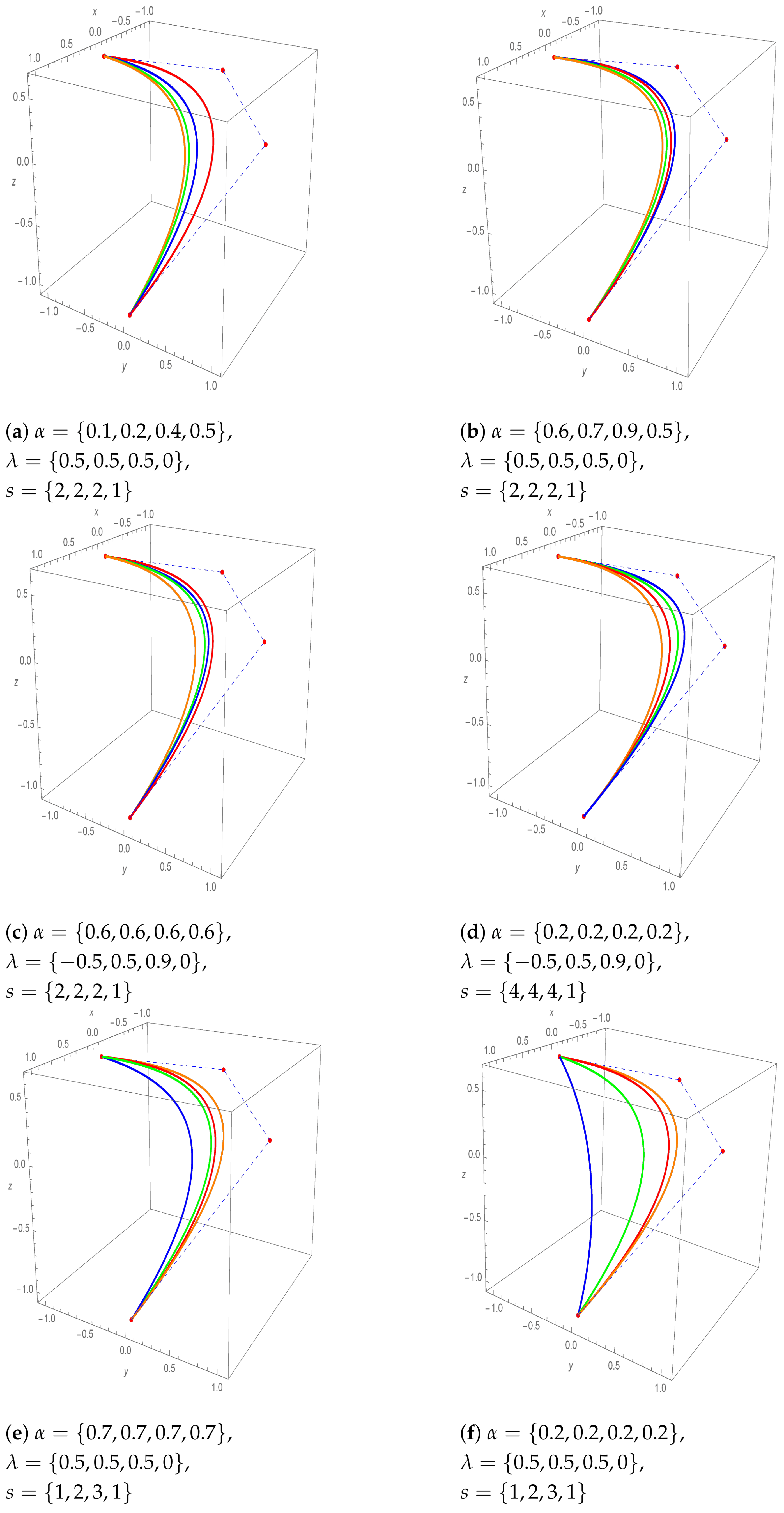
In this subsection, we illustrate $(\alpha ,\lambda ,s)$-Bézier space curves with Figure 6 and Figure 7. The red curves in Figure 6 are drawn using the classical Bernstein polynomial bases. As evident from the graphs, variations in the parameters allow the curves to shift closer to or farther from the control points in comparison to the classical one.

Figure 6. Space curves with 3rd degree. The set of control points is {(1, 0, −1), (0, 1, 0.2), (−1, 0, 0.4), (0, −1, 0.6)}. Curve colors are organized as orange, green, blue, and red, according to the order in which the parameters are given. In each figure, red indicates the classical Bézier curves.

Figure 6. Space curves with 3rd degree. The set of control points is {(1, 0, −1), (0, 1, 0.2), (−1, 0, 0.4), (0, −1, 0.6)}. Curve colors are organized as orange, green, blue, and red, according to the order in which the parameters are given. In each figure, red indicates the classical Bézier curves.

In Figure 7, we plot our curves using $(\alpha ,\lambda ,s)$-Bernstein polynomials of degree 12, observing that changes in the value of $\lambda$ do not seem to affect the shape of the curve much. This is due to the fact that as the degree increases, the effect of $\lambda$ decreases (see (4)).

Figure 7. Space curves with 12th degree. The set of control points is (1, 0, 0), (0.8, 0.6, 0.2), (0.4, 0.9, 0.4), (0, 1, 0.6), (−0.4, 0.9, 0.8), (−0.8, 0.6, 1), (−1, 0, 1.2), (−0.8, −0.6, 1.4), (−0.4, −0.9, 1.6), (0, −1, 1.8), (0.4, −0.9, 2), (0.8, −0.6, 2.2), (1, 0, 2.4). Curve colors are organized as orange, green, blue, and red, according to the order in which the parameters are given. In each figure, red indicates the classical Bézier curves.

Figure 7. Space curves with 12th degree. The set of control points is (1, 0, 0), (0.8, 0.6, 0.2), (0.4, 0.9, 0.4), (0, 1, 0.6), (−0.4, 0.9, 0.8), (−0.8, 0.6, 1), (−1, 0, 1.2), (−0.8, −0.6, 1.4), (−0.4, −0.9, 1.6), (0, −1, 1.8), (0.4, −0.9, 2), (0.8, −0.6, 2.2), (1, 0, 2.4). Curve colors are organized as orange, green, blue, and red, according to the order in which the parameters are given. In each figure, red indicates the classical Bézier curves.

4. (α, λ, s)-Bézier Surfaces and Their Properties

We now define the tensor product $(\alpha ,\lambda ,s)$-Bézier surfaces with degree $r_1\times r_2$ as follows:

$${\displaystyle C^{({\alpha }_1,{\lambda }_1,s_1;{\alpha }_2,{\lambda }_2,s_2)}(z_1,z_2;\mathbf{P})=\sum _{i_1=0}^{r_1}\sum _{i_2=0}^{r_2}{q}_{r_1,i_1}^{{\alpha }_1,{\lambda }_1,s_1}\left(z_1\right)q_{r_2,i_2}^{{\alpha }_2,{\lambda }_2,s_2}\left(z_2\right){\mathbf{P}}_{i_1,i_2},}$$

(32)

where $(z_1,z_2)\in [0,1]\times [0,1]$, ${\lambda }_1$, ${\lambda }_2\in [-1,1]$, $z_1$, $z_2\in [0,1]$, $s_1$ and $s_2$ are positive integers, $\{{\mathbf{P}}_{i_1,i_2}={\mathbf{P}}_{i_1,i_2}(x_k,y_k,z_k)\in R^3:i_1=0,1,...,r_1,i_2=0,1,...,r_2$, $1\le k\le (r_1+1)\times (r_2+1)\}$ is the set of control points, and $q_{r_1,i_1}^{{\alpha }_1,{\lambda }_1,s_1}\left(z_1\right)$ and $q_{r_2,i_2}^{{\alpha }_2,{\lambda }_2,s_2}\left(z_2\right)$ are defined as (6). We obtain a net by joining the adjacent control points in row or column. This net is called the control net of the tensor product $(\alpha ,\lambda ,s)$-Bézier surfaces which satisfy the following properties:

(S.1)

Corner point interpolation property. $(\alpha ,\lambda ,s)$-Bézier surfaces pass through all four corner control points of the control net denoted by ${\mathbf{P}}_{0,0}$, ${\mathbf{P}}_{0,r_2}$, ${\mathbf{P}}_{r_1,0}$, and ${\mathbf{P}}_{r_1,r_2}$, where by (5)

$$\begin{array}{c}\hfill {\mathbf{P}}_{0,0}=C^{({\alpha }_1,{\lambda }_1,s_1;{\alpha }_2,{\lambda }_2,s_2)}(0,0),{\mathbf{P}}_{0,r_2}=C^{({\alpha }_1,{\lambda }_1,s_1;{\alpha }_2,{\lambda }_2,s_2)}(0,1),\\ \hfill {\mathbf{P}}_{r_1,0}=C^{({\alpha }_1,{\lambda }_1,s_1;{\alpha }_2,{\lambda }_2,s_2)}(1,0),{\mathbf{P}}_{r_1,r_2}=C^{({\alpha }_1,{\lambda }_1,s_1;{\alpha }_2,{\lambda }_2,s_2)}(1,1).\end{array}$$

(S.2)

Reducibility: By Remark 1, for ${\alpha }_1={\alpha }_2=1$ and ${\lambda }_1={\lambda }_2=0$, we obtain the classical tensor product Bézier surfaces.

(S.3)

Convex hull property: Since $C^{({\alpha }_1,{\lambda }_1,s_1;{\alpha }_2,{\lambda }_2,s_2)}$ is the convex combination of the points ${\mathbf{P}}_{i_1,i_2}$, it lies in the convex hull of its control net.

(S.4)

Isoparametric curves property: The $z_1$-parameter curve of a tensor product of a $(\alpha ,\lambda ,s)$-Bézier surface is a $(\alpha ,\lambda ,s)$-Bézier curve of degree $r_1$ with $z_2$ fixed; that is, $z_2$ is a real constant in [0, 1], say $c_2$, is represented as

$$\begin{array}{cc}\hfill C^{({\alpha }_1,{\lambda }_1,s_1;{\alpha }_2,{\lambda }_2,s_2)}(z_1,c_2)& {\displaystyle =\sum _{i_1=0}^{r_1}\left(\sum _{i_2=0}^{r_2}{\mathbf{P}}_{i_1,i_2}{q}_{r_2,i_2}^{{\alpha }_2,{\lambda }_2,s_2}\left(c_2\right)\right)q_{r_1,i_1}^{{\alpha }_1,{\lambda }_1,s_1}\left(z_1\right)}\hfill \\ \hfill & {\displaystyle =\sum _{i_1=0}^{r_1}{q}_{r_1,i_1}^{{\alpha }_1,{\lambda }_1,s_1}\left(z_1\right)a_{i_1}\left(c_2\right),}\hfill \end{array}$$

where $z_1\in [0,1]$, ${\displaystyle a_{i_1}\left(c_2\right)=\sum _{i_2=0}^{r_2}{q}_{r_2,i_2}^{{\alpha }_2,{\lambda }_2,s_2}\left(c_2\right){\mathbf{P}}_{i_1,i_2}}$, and $a_0\left(c_2\right),a_1\left(c_2\right),...,a_{r_1}\left(c_2\right)$ are the control points of the $z_1$-parameter $(\alpha ,\lambda ,s)$-Bézier curve on a tensor product $(\alpha ,\lambda ,s)$-Bézier surface. the $z_2$-parameter $(\alpha ,\lambda ,s)$-Bézier curve on a tensor product $(\alpha ,\lambda ,s)$-Bézier surface is computed similarly. Now, one can easily obtain the boundary curves of an $(\alpha ,\lambda ,s)$-Bézier surface by computing $C^{({\alpha }_1,{\lambda }_1,s_1;{\alpha }_2,{\lambda }_2,s_2)}(0,z_2)$, $C^{({\alpha }_1,{\lambda }_1,s_1;{\alpha }_2,{\lambda }_2,s_2)}(1,z_2)$, $C^{({\alpha }_1,{\lambda }_1,s_1;{\alpha }_2,{\lambda }_2,s_2)}(z_1,0)$, and $C^{({\alpha }_1,{\lambda }_1,s_1;{\alpha }_2,{\lambda }_2,s_2)}(z_1,1).$

(S.5)

Partition of unity: The sum of $q_{r_1,i_1}^{{\alpha }_1,{\lambda }_1,s_1}\ast q_{r_2,i_2}^{{\alpha }_2,{\lambda }_2,s_2}$ is one, that is,

$${\displaystyle \sum _{i_1=0}^{r_1}\sum _{i_2=0}^{r_2}{q}_{r_2,i_2}^{{\alpha }_2,{\lambda }_2,s_2}\left(z_2\right)q_{r_1,i_1}^{{\alpha }_1,{\lambda }_1,s_1}\left(z_1\right)=\left(\sum _{i_2=0}^{r_2}{q}_{r_2,i_2}^{{\alpha }_2,{\lambda }_2,s_2}\left(z_2\right)\right)\left({\displaystyle \sum _{i_1=0}^{r_1}{q}_{r_1,i_1}^{{\alpha }_1,{\lambda }_1,s_1}\left(z_1\right)}\right)=1}$$

since, by Lemma 1, ${\displaystyle \sum _{i_1=0}^{r_1}{q}_{r_1,i_1}^{{\alpha }_1,{\lambda }_1,s_1}\left(z_1\right)=1}$ and ${\displaystyle \sum _{i_2=0}^{r_2}{q}_{r_2,i_2}^{{\alpha }_2,{\lambda }_2,s_2}\left(z_2\right)=1.}$

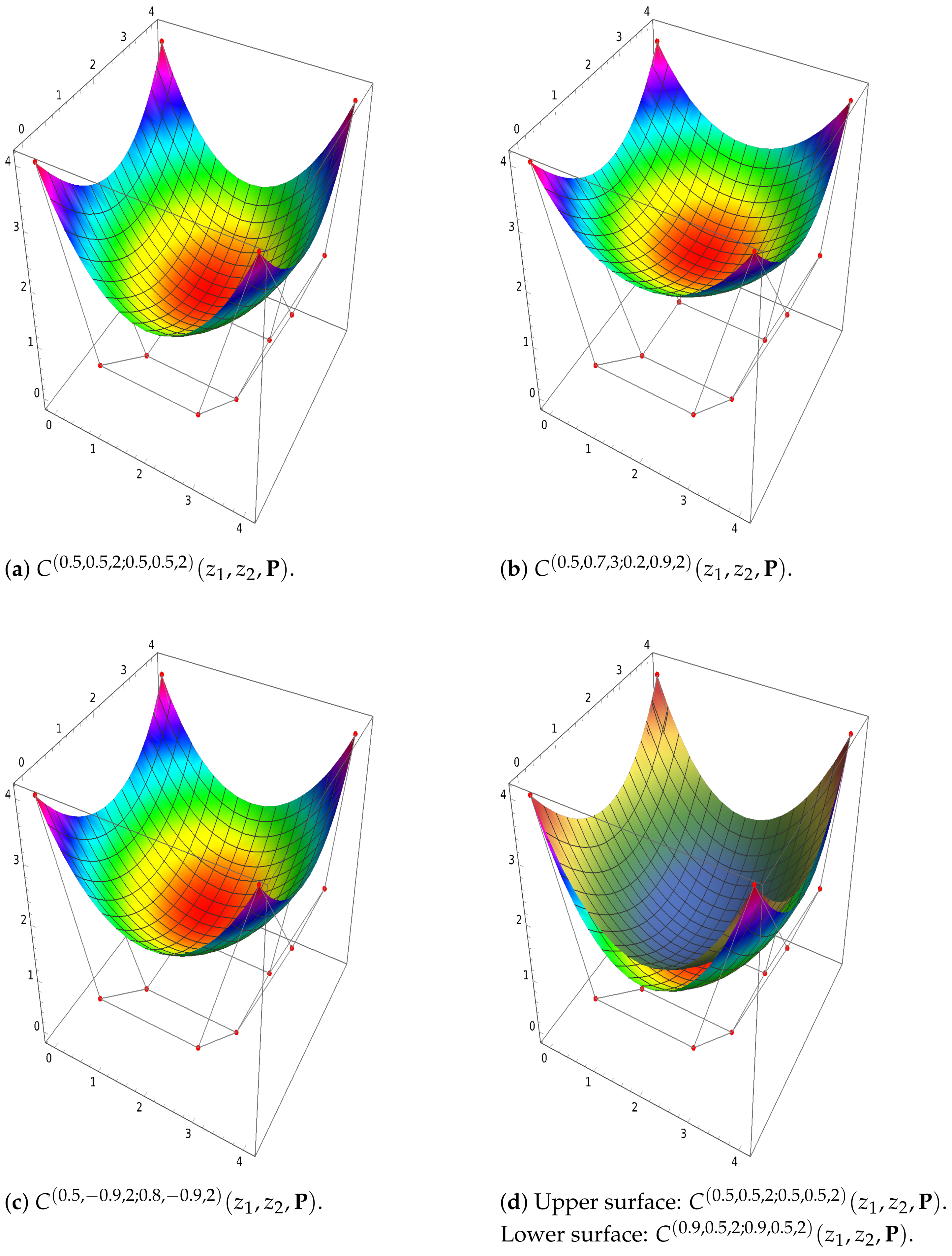
In Figure 8, we demonstrate the effects of the shape parameters in $(\alpha ,\lambda ,s)$-Bézier surfaces in (a)–(c) separately, whereas in (d), two different surfaces are sketched simultaneously.

In Figure 9, an $(\alpha ,\lambda ,s)$-Bézier surface with the shape parameters $\alpha =0.5$, $\lambda =0.9$, and $s=2$ is compared to (a) a classical Bézier surface; (b) an $\alpha$-Bézier surface with $\alpha =0.5$, and (c) a $\lambda$-Bézier surface with $\lambda =0.9$.

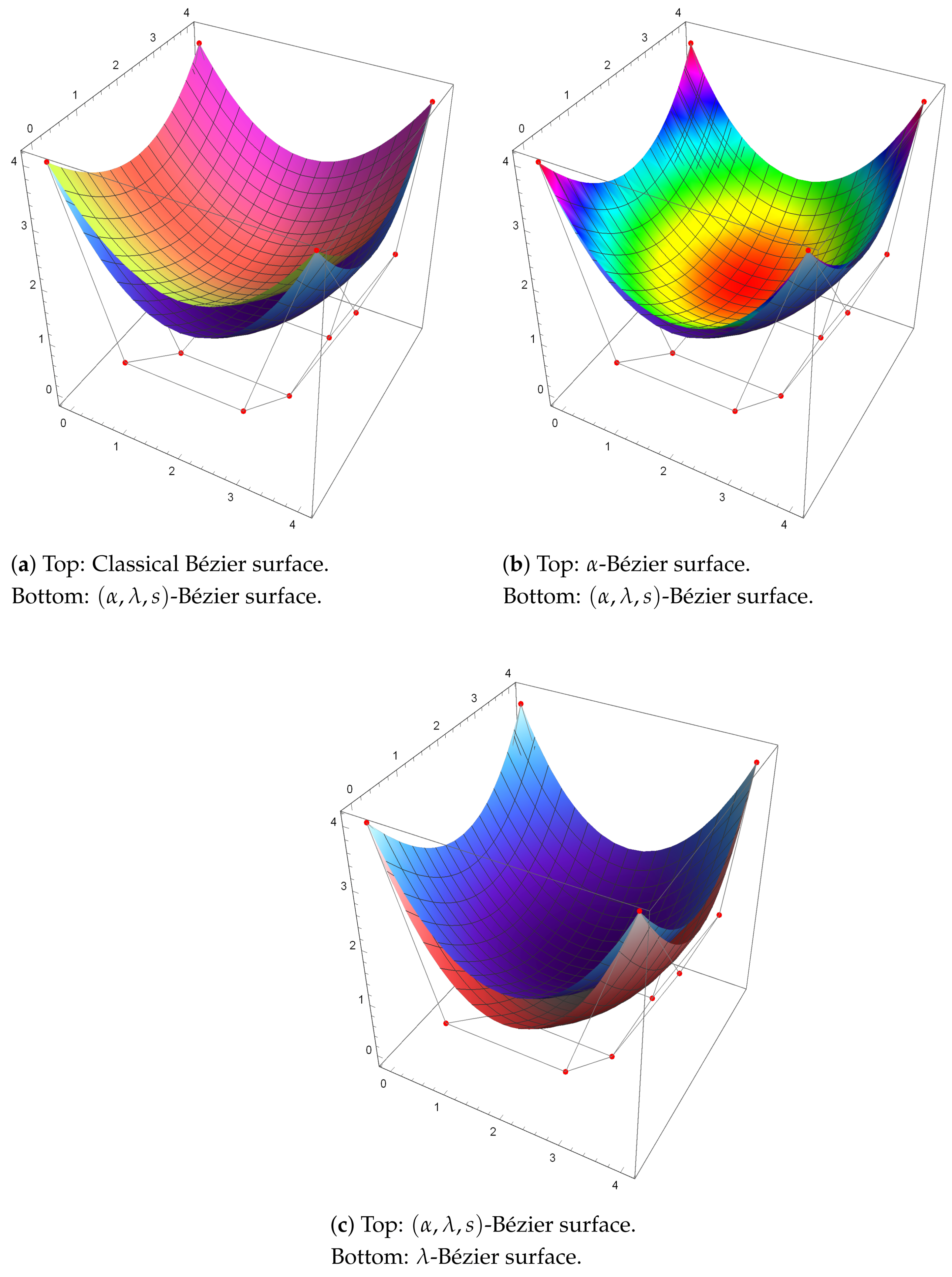
From top to bottom, Figure 10 visualizes the classical, $\alpha$-, $(\alpha ,\lambda ,s)$-, and $\lambda$-Bézier surfaces all in one. In each part, the same surfaces can be observed from different viewpoints.

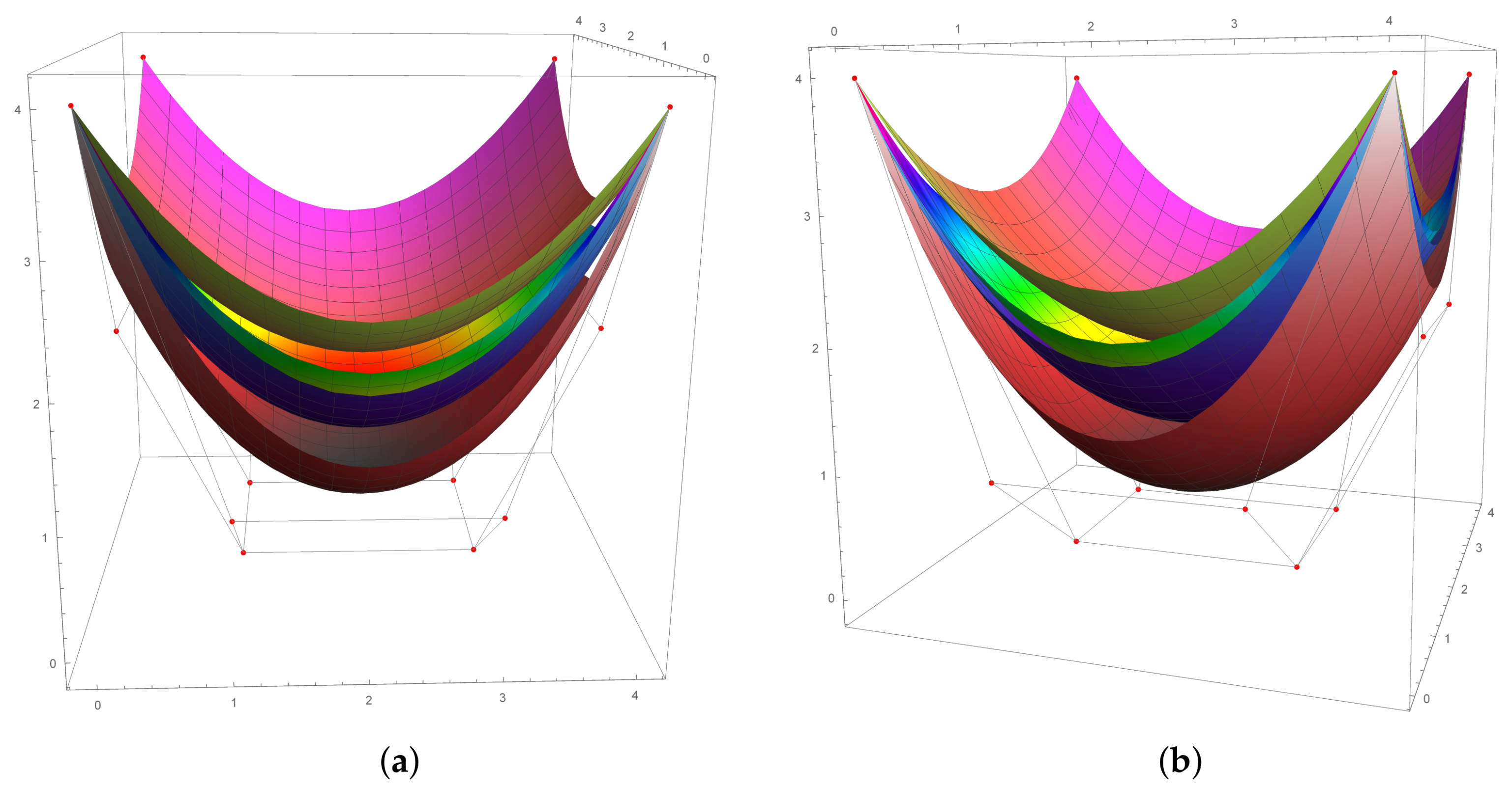
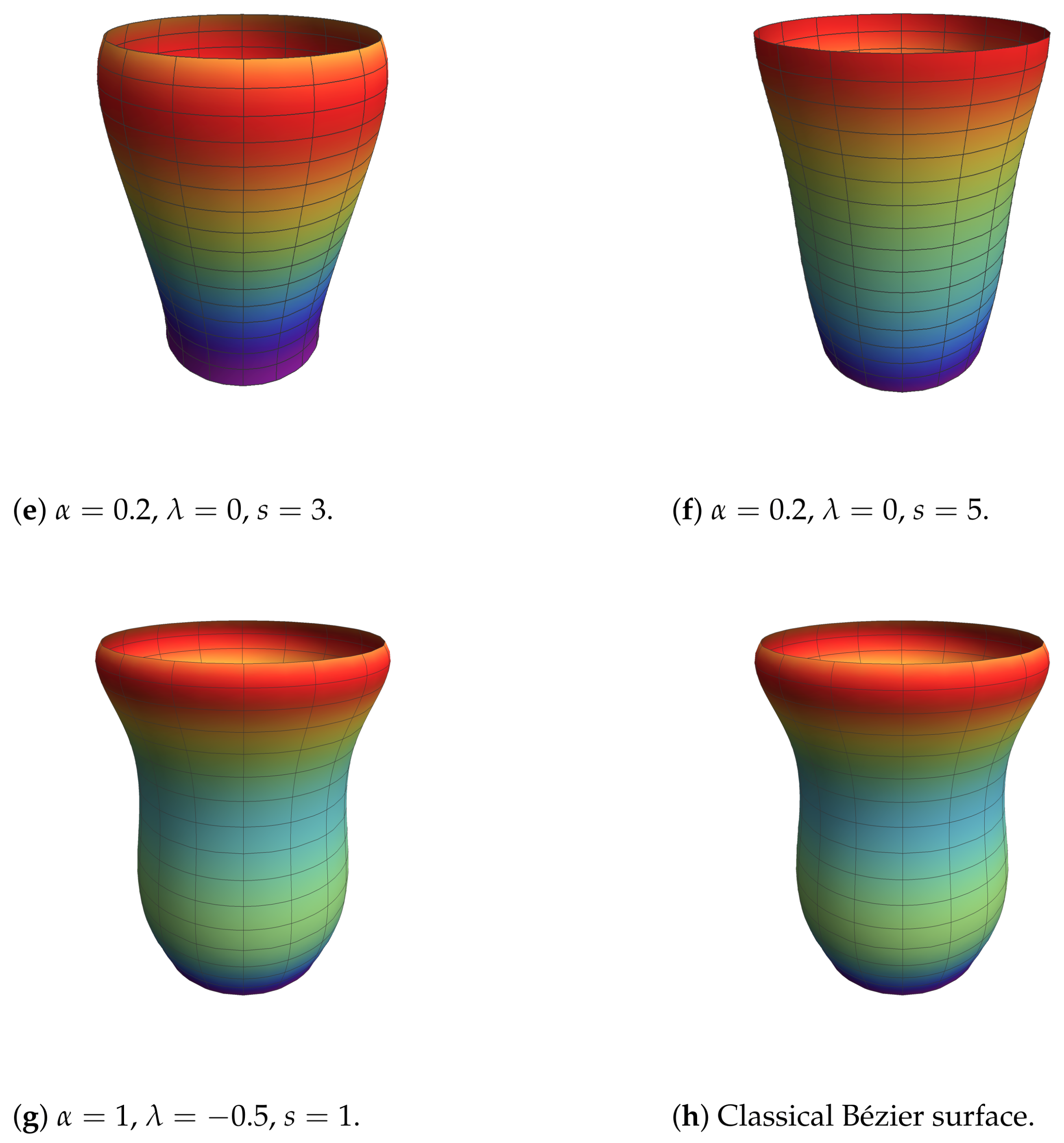
Figure 11 shows that the parameter variations yield a broad spectrum of surface shapes, showcasing the potential for designing complex geometries. Comparisons with the classical Bézier surface in part (H) reveal the significant improvements in flexibility and shape diversity offered by the $(\alpha ,\lambda ,s)$-Bézier framework.

5. Conclusions

This paper introduces a novel approach to curve and surface modeling through the generalized $(\alpha ,\lambda ,s)$-Bernstein basis. By incorporating three shape parameters—$\alpha$, $\lambda$, and s—into the traditional Bernstein basis, we developed a powerful tool that significantly enhances the flexibility and control available in computer-aided geometric design. The resulting $(\alpha ,\lambda ,s)$-Bézier curves and surfaces retain the essential geometric properties of their classical counterparts, such as convex hull containment and endpoint interpolation, while offering advanced capabilities for shape manipulation.

The versatility of the $(\alpha ,\lambda ,s)$-Bernstein basis opens up new possibilities for various applications in fields ranging from industrial design to digital graphics and beyond. Its ability to maintain geometric integrity while allowing for precise adjustments makes it an invaluable asset in scenarios where traditional Bézier curves fall short. Moreover, the introduction of multiple shape parameters offers a more comprehensive framework for addressing complex design challenges, ultimately contributing to more refined and efficient modeling processes.

As this research advances, future work may explore the integration of the $(\alpha ,\lambda ,s)$-Bernstein basis with other curve and surface modeling techniques, as well as its potential applications in real-time rendering and animation. The findings presented in this paper lay the groundwork for these explorations, highlighting the potential of the $(\alpha ,\lambda ,s)$-Bernstein basis to become a cornerstone of modern geometric design.