Safety of Uncertain Session Types with Interval Probability

Abstract

In this article, we introduce and study a new kind of multiparty session type for a probabilistic process calculus that incorporates two forms of choice: probabilistic and nondeterministic. The main novelty of our approach is the use of interval probabilities in a type system in order to deal with uncertainty in a probabilistic process calculus. We present a decidable proof system that ensures deadlock freedom, type preservation and type safety, even when several types can be assigned to a process. The new typing system represents a conservative extension of the standard typing system based on multiparty session types (removing the probabilities from processes does not affect their well-typedness). We also define a probabilistic bisimulation between processes that are typed by using the same sorting and typing.

1. Introduction

Session types represent a type discipline used to describe communication-centric systems in the framework of process calculi. Involving concurrent processes, session types guarantee that message-passing communication follows predefined protocols, implementing given (multiparty) session protocols without errors. In this way, the session types describe statically the communication protocols, and well-typedness ensures that the behavior is in accordance with these protocols at runtime.

The theory of session types operates under the assumption of no system errors (e.g., failure at transport level), and does not account for tolerance of interactions or variability of parameters in a communication protocol [1]. In fact, most of the work on session types has focused on error-free (and non-probabilistic) scenarios; only recently were published some papers focusing on failures [2,3,4,5,6,7]. However, many real-life communication and concurrent message-passing systems involve various uncertainties, and so they are generally probabilistic. In the real world, these systems involving network and embedded equipment exhibit different kinds of uncertainty in their behavior as a result of some random physical parameters. Probability theory and stochastic processes provide the mathematical foundation for analyzing uncertain and random phenomena. The use of a probabilistic approach can be more realistic and helpful in analyzing the communication-centric systems. The use of probabilities in session types was presented recently in some articles [8,9,10,11,12,13,14].

In this article, we introduce new multiparty session types for a probabilistic process calculus that incorporates two forms of choice: probabilistic and nondeterministic. The main novelty of our approach is the use of interval probabilities in a type system in order to deal with uncertainty in a probabilistic process calculus; in this way, several processes can be well-typed by the same type and several types can be assigned to the same process. We present a decidable proof system that ensures deadlock freedom, type preservation and type safety.

The concept of interval probability is introduced to generalize classical probability for describing uncertainty in general. Such intervals of probabilities are mentioned in early articles [15,16]. More recently, interval probability has been used in [17] for stochastic hybrid systems to manage uncertainty and to develop an efficient formal analysis and control synthesis of (discrete-time) stochastic hybrid systems with linear dynamics. Using the Interval Markov Decision Processes (labelling transitions by intervals of probabilities) as an abstract model, the authors present a robust strategy against the uncertainties of the real-world hybrid systems. The uncertainties are viewed as the nondeterministic choice of a feasible transition probability from one state to another (under a given action); in this way, specific reachability and safety problems are solved.

As usual for multiparty session types, we consider a top-down approach where we utilize global types (that describe the interactions among distributed processes) to enforce communication safety and the local types (obtained by projection from global types) to statically type-check the processes. If processes are well-typed, then they correctly interact as prescribed by a multiparty session protocol. To formally describe these systems, we use interval probabilities in our type system in order to deal with uncertainty in the probabilistic process calculus. In this way, we obtain a formal model for complex communication-centric protocols to describe and analyze their behavior by involving tolerance to inherent uncertainties provided by certain random physical parameters. We use local and global types that incorporate interval probabilities, and allow processes to incorporate two forms of choice: probabilistic internal and nondeterministic external. Note that, in general, the deterministic behavior cannot be replaced by a probabilistic behavior (only in some cases is valid to assume that a probabilistic mechanism governs a nondeterministic choice). This is also due to the fact that the behavior produced by nondeterministic choices is unpredictable, while the one produced by probabilistic is predictable in the long run. Thus, the probabilistic and nondeterministic choices need to be treated separately [18].

The paper follows the standard way of dealing with session types. Section 2 presents the syntax and semantics of our probabilistic calculus incorporating two types of choice (probabilistic and nondeterministic); we use a running example to illustrate the key aspects. Section 3 introduces the global and local types, together with their connection established by a projection. Section 4 presents the new probabilistic typing system that ensures deadlock freedom, type preservation and type safety, even when several types can be assigned to a process. The new typing system represents a conservative extension; removing the probabilities from processes does not affect their well-typedness. Section 4 also defines the probabilistic relations between processes that are typed according to specific sorting and typing, and a bisimulation between processes that are typed under the same sorting and typing. Section 5 presents the conclusions, and discusses other approaches that used probabilities in typing systems.

This is a revised and extended version of [19]. In addition to some improvements in motivation, related work and by including the missing proofs, the most significant technical differences between this article and its conference version are as follows: (i) defining a probabilistic relation between processes that are typed under the same sorting and typing and corresponding definitions when the probabilities are erased; (ii) proving that the previous relation is an equivalence and that there exist several such relations that can relate two processes; (iii) defining and studying bisimulations between processes by also taking into account their types and interval probability.

2. Probabilistic Multiparty Session Calculus

Using similar notations as for the calculus presented in [20], we propose a probabilistic extension of a synchronous multiparty session process calculus. However, taking inspiration from [21], we simplify the syntax by omitting session initiations and dedicated input/output prefixes. Our calculus allows processes to incorporate two forms of choice: probabilistic internal choice and nondeterministic external choice.

2.1. Syntax

A session between multiple parties is basically a series of their interactions. In order to establish a session, the involved parties should use a shared public name that is employed to create fresh session channels that will be used only for communication between them.

Table 1. Syntax of the probabilistic multiparty session calculus.

Processes
$P,Q$	$::=$	$c\left[r\right]{\oplus }_{i\in I}\langle p_i:l_i\left(v_i\right).P_i\rangle$	$(\mathrm{selection}\mathrm{towards}\mathrm{role}r,I\ne \varnothing ,{\sum }_{i\in I}{p}_i=1)$
	|	$c\left[r\right]{\&}_{i\in I}\{l_i\left(x_i\right).P_i\}$	(branching from role r, $I\ne \varnothing$)
	|	$\mathsf{def}D\mathsf{in}P|$$X\left(\tilde{v}\tilde{c}\right)$	(process definition & process call)
	|	$P\mid Q|$$\left(\nu s\right)P$	(parallel & restriction)
	|	$\mathbf{0}|$$\mathsf{err}$	(inaction & error)
Declarations
D	$::=$	$X\left(\tilde{x}\right)=P$	(process declaration)
Contexts
$\mathcal{E}$	$::=$	$\left[\right]|$$\left(\nu s\right)\mathcal{E}|$$\mathsf{def}D\mathsf{in}\mathcal{E}|$$\mathcal{E}\mid P$	(evaluation context)
Channels
c	$::=$	x| $s\left[r\right]$	(variable, channel with role r)
Values
v	$::=$	$c\left|true\right|false|$$3|\dots$	(channel, base value)

presents the syntax of our probabilistic calculus, where we use p for probabilities, c and s for channels, v for values, x for variables, l for labels, r for roles and X for the process variables appearing in recursive processes.

The selection process $c\left[r\right]{\oplus }_{i\in I}\langle p_i:l_i\left(v_i\right).P_i\rangle$ uses channel c to send with probability $p_i$ towards role r the labelled value $l_i\left(v_i\right)$, and then it behaves according to process $P_i$. Since all the labels in the set ${\left\{l_i\right\}}_{i\in I}$ are unique by construction, the selection process has I possible continuations. We only impose that the sum of probabilities appearing in a selection is 1, without further constraints or connections with other probabilities appearing in a process. In a similar manner, the branching process $c\left[r\right]{\&}_{i\in I}\{l_i\left(x_i\right).P_i\}$ uses channel c to receive from role r a labelled value. If the value received has label $l_i$, the branching process behaves according to process $P_i$ in which the received value replaces all free occurrences of the variable $x_i$. Note that the branching process is the only one that bounds variables, namely each variable $x_i$ is bound within the scope of $P_i$. The set of free channels and free variables of a process P (namely those not bound in the branching process) are denoted by $\mathit{fc}\left(P\right)$ and $\mathit{fv}\left(P\right)$, respectively, while the set of all processes is denoted by $\mathcal{P}$.

The restriction process $\left(\nu s\right)P$ represents a process P to which the scope of session s is constrained. Process definition $\mathsf{def}D\mathsf{in}P$ and process call $X\left(\tilde{v}\tilde{c}\right)$ are used to define recursive behaviors. If D from the process definition has the form $X\left(\tilde{x}\right)=P$, then the process call $X\left(\tilde{v}\tilde{c}\right)$ behaves as P in which $\tilde{v}\tilde{c}$ are used to replace the variables $\tilde{x}$. Similar to the approach of [20], we allow only closed process declarations in which the process declaration $X\left(\tilde{x}\right)=P$ is such that $\mathit{fc}\left(P\right)=\varnothing$ and $\mathit{fv}\left(P\right)\subseteq \tilde{x}$. The inaction process $\mathbf{0}$ is a process that does nothing, while the parallel process $P|Q$ allows the concurrent processes P and Q to communicate on a shared channel. The error process err marks the fact that we have an unsuccessful communication. Processes containing holes are used as evaluation contexts, while a communication channel c is either a variable x or a channel $s\left[r\right]$ for role r in a session s, as in [22]. Values v used in processes can be Boolean, integers or strings.

Example 1.

In what follows, we describe a process that outlines a straightforward survey poll in which $\mathrm{Alice}$ either answers $\mathrm{Bob}$’s questions or opts out. $\mathrm{Bob}$ can conclude the poll if satisfied with the responses received or proceed with additional polling questions. Similar to the scenario described in [23], $\mathrm{Alice}$ and $\mathrm{Bob}$ express their preferences and receive others’ choices, each accompanied by numerical probabilities. These probabilities establish a clear numerical scale for responses.

The starting system is as follows:

$$\mathrm{System}=\left(\nu \mathrm{s}\right)\left(\mathrm{Bob}\right|\left(\nu \mathrm{phoneA}\right)\left(\nu \mathrm{imA}\right)\mathrm{Alice}).$$

The session that involves the parallel processes of $\mathrm{Alice}$ and $\mathrm{Bob}$ is denoted by $\mathrm{s}$. This session encompasses two roles: ${\mathrm{r}}_{\mathrm{A}}$ assigned to $\mathrm{Alice}$ and ${\mathrm{r}}_{\mathrm{B}}$ assigned to $\mathrm{Bob}$. Thus, within this session, $\mathrm{Alice}$ and $\mathrm{Bob}$ communicate by using channels identified by roles $\mathrm{s}\left[{\mathrm{r}}_{\mathrm{A}}\right]$ and $\mathrm{s}\left[{\mathrm{r}}_{\mathrm{B}}\right]$, respectively. Additionally, $\mathrm{phoneA}$ and $\mathrm{imA}$ are sessions in which $\mathrm{Alice}$ and $\mathrm{Bob}$ can interact; these sessions can be established by performing communications within session $\mathrm{s}$. It is important to note that initially the scopes of $\mathrm{phoneA}$ and $\mathrm{imA}$ are limited to $\mathrm{Alice}$, as $\mathrm{Bob}$ is informed later if he needs to join one of these sessions. The variable ${\mathrm{x}}_{\mathrm{q}}$ appearing in ${\mathrm{A}}_1$ of $\mathrm{Alice}$ is used to wait for a question $\mathrm{q}$ from $\mathrm{Bob}$ to which she can answer or not.

$\mathrm{Alice}=\mathsf{def}\mathrm{A}\left(\mathrm{y}\right)={\mathrm{A}}_1\mathsf{in}{\mathrm{A}}_2$, where the definitions of ${\mathrm{A}}_1$ and ${\mathrm{A}}_2$ are as follows:

$$\begin{array}{cc}{\mathrm{A}}_1=\mathrm{y}\left[{\mathrm{r}}_{\mathrm{B}}\right]\&\{\mathrm{talk}\left({\mathrm{x}}_{\mathrm{q}}\right).\mathrm{y}\left[{\mathrm{r}}_{\mathrm{B}}\right]\oplus \langle & 0.6:\mathrm{yes}\left({\mathrm{x}}_{\mathrm{q}}\right).\mathrm{A}\left(\mathrm{y}\right),\\ & 0.3:\mathrm{no}\left({\mathrm{x}}_{\mathrm{q}}\right).\mathrm{A}\left(\mathrm{y}\right),\\ & 0.1:\mathrm{quit}\left({\mathrm{x}}_{\mathrm{q}}\right).\mathbf{0}\rangle ),\\ \mathrm{quit}.\mathbf{0}\};& \end{array}$$

$$\begin{array}{cc}{\mathrm{A}}_2=\mathrm{s}\left[{\mathrm{r}}_{\mathrm{A}}\right]\left[{\mathrm{r}}_{\mathrm{B}}\right]\oplus \langle & 0.6:\mathrm{phone}\left(\mathrm{phoneA}\right).\mathrm{A}\left(\mathrm{phoneA}\left[{\mathrm{r}}_{\mathrm{A}}\right]\right),\hfill \\ & 0.35:\mathrm{im}\left(\mathrm{IMIdA}\right).\mathrm{A}\left(\mathrm{imA}\left[{\mathrm{r}}_{\mathrm{A}}\right]\right),\hfill \\ & 0.05:\mathrm{not}\left(\mathrm{no}\right).\mathbf{0}\rangle .\hfill \end{array}$$

$\mathrm{Bob}=\mathsf{def}\mathrm{B}(\mathrm{y},\mathrm{q})={\mathrm{B}}_1\mathsf{in}{\mathrm{B}}_2$, where the definitions of ${\mathrm{B}}_1$ and ${\mathrm{B}}_2$ are as follows:

$$\begin{array}{ccc}{\mathrm{B}}_1=\mathrm{y}\left[{\mathrm{r}}_{\mathrm{A}}\right]\oplus \langle \hfill & 0.95:\mathrm{talk}\left(\mathrm{q}\right).\mathrm{y}\left[{\mathrm{r}}_{\mathrm{A}}\right]\&\{\hfill & \mathrm{yes}\left(\mathrm{q}\right).\mathrm{B}(\mathrm{y},\mathrm{next}(\mathrm{q}\left)\right),\hfill \\ & & \mathrm{no}\left(\mathrm{q}\right).\mathrm{B}(\mathrm{y},\mathrm{next}(\mathrm{q}\left)\right),\hfill \\ & & \mathrm{unsure}\left(\mathrm{q}\right).\mathrm{B}(\mathrm{y},\mathrm{next}(\mathrm{q}\left)\right),\hfill \\ & & \mathrm{quit}\left(\mathrm{q}\right).\mathbf{0}\},\hfill \\ & 0.05:\mathrm{quit}.\mathbf{0}\rangle ;\hfill & \end{array}$$

$$\begin{array}{cc}{\mathrm{B}}_2=\mathrm{s}\left[{\mathrm{r}}_{\mathrm{B}}\right]\left[{\mathrm{r}}_{\mathrm{A}}\right]\&\{& \mathrm{phone}\left({\mathrm{x}}_{\mathrm{A}}\right).\mathrm{B}({\mathrm{x}}_{\mathrm{A}}\left[{\mathrm{r}}_{\mathrm{B}}\right],{\mathrm{q}}_1),\hfill \\ & \mathrm{im}\left({\mathrm{x}}_{\mathrm{A}}^{\prime }\right).\mathrm{B}({\mathrm{x}}_{\mathrm{A}}^{\prime }\left[{\mathrm{r}}_{\mathrm{B}}\right],{\mathrm{q}}_1),\hfill \\ & \mathrm{not}\left({\mathrm{x}}_{\mathrm{A}}^{\prime \prime }\right).\mathbf{0}\}.\hfill \end{array}$$

The concurrent behavior of processes $\mathrm{Alice}$ and $\mathrm{Bob}$ is explained through their interaction.

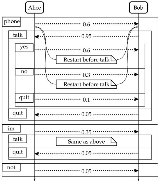
• Initial decision: $\mathrm{Alice}$ uses the channel with role $\mathrm{s}\left[{\mathrm{r}}_{\mathrm{A}}\right]$ in order to decide how to respond to the poll: by phone, instant messaging or by deferring the response. Probabilities are assigned to each option, indicating $\mathrm{Alice}$’s choice.
• Phone communication: If $\mathrm{Alice}$ chooses the $\mathrm{phone}$ option, communication occurs through a unique session channel ($PhoneNoA$) representing $\mathrm{Alice}$’s phone number.
• $\mathrm{Bob}$’s interaction: $\mathrm{Bob}$ initiates the interaction by invoking $\mathrm{B}({\mathrm{x}}_{\mathrm{A}}\left[{\mathrm{r}}_{\mathrm{B}}\right],{\mathrm{q}}_1)$, where ${\mathrm{x}}_{\mathrm{A}}$ becomes $\mathrm{phoneA}$ after communication. Here, ${\mathrm{q}}_1$ represents the first question for $\mathrm{Alice}$ to answer using the following labels: $\mathrm{yes}$, no, $\mathrm{unsure}$ or $\mathrm{quit}$. $\mathrm{Alice}$ excludes the $\mathrm{unsure}$ option for this question, as she considers it inapplicable to the question at hand.
• Question–answer sequence: After receiving an answer, $\mathrm{Bob}$ proceeds to the next question in the list (represented by $\mathrm{next}$).
• Exiting the poll: Both processes are able to get out of the poll by selecting either the $\mathrm{quit}$ or $\mathrm{not}$ label. These options have low probabilities, indicating a low likelihood of being chosen during the survey poll.

2.2. Operational Semantics

If a name s is not in $\mathit{fc}\left(P\right)$, then we cannot find any role r such that $s\left[r\right]$ exists within $\mathit{fc}\left(P\right)$. Additionally, we use $dpv\left(D\right)$ to represent all process variables that are declared in D and $fpv\left(P\right)$ to represent all process variables that appear as free variables in P.

Operational semantics is defined by using the structural congruence as its foundation:

$P|Q\equiv Q|P\left(P\right|Q\left)\right|R\equiv P\left|\right(Q\left|R\right)$    $P|\mathbf{0}\equiv P(\nu s)\mathbf{0}\equiv \mathbf{0}\mathsf{def}D\mathsf{in}\mathbf{0}\equiv \mathbf{0}$

$\left(\nu s\right)\left(\nu s^{\prime }\right)P\equiv \left(\nu s^{\prime }\right)\left(\nu s\right)P$      $\left(\nu s\right)P|Q\equiv (\nu s\left)\right(P\left|Q\right)(\mathrm{if}s\notin \mathit{fc}(Q\left)\right)$

$\mathsf{def}D\mathsf{in}\left(\nu s\right)P\equiv \left(\nu s\right)\mathsf{def}D\mathsf{in}P(\mathrm{if}s\notin \mathit{fc}(D\left)\right)$

1ex $\mathsf{def}D\mathsf{in}\left(P\right|Q)\equiv (\mathsf{def}D\mathsf{in}P\left)\right|Q$ $\left(\mathrm{if}dpv\right(D)\cap fpv(Q)=\varnothing )$

$\mathsf{def}D\mathsf{in}\mathsf{def}{D}^{\prime }\mathsf{in}P\equiv \mathsf{def}{D}^{\prime }\mathsf{in}\mathsf{def}D\mathsf{in}P$

$(\mathrm{if}(dpv\left(D\right)\cup fpv\left(D\right))\cap dpv\left(D^{\prime }\right)$ $=(dpv\left(D^{\prime }\right)\cup fpv\left(D^{\prime }\right))\cap dpv\left(D\right)=\varnothing )$

$P\equiv Q$ implies $\mathcal{E}\left[P\right]\equiv \mathcal{E}\left[Q\right]$.

For our probabilistic calculus, operational semantics is defined inductively according to

Table 2. Operational semantics of the probabilistic multiparty session calculus.

$s\left[r_1\right]\left[r_2\right]{\oplus }_{j\in J}\langle p_j:l_j\left(v_j\right).P_j\rangle \mid s\left[r_2\right]\left[r_1\right]{\&}_{i\in I}\{l_i\left(x_i\right).P_i^{\prime }\}$${\to }_{p_k}{P}_k\mid P_k^{\prime }\{\widetilde{v_k}/\widetilde{x_k}\}$ (if $k\in J\subseteq I$)	(Com)
$\mathsf{def}X\left(\tilde{x}\right)=P\mathsf{in}\left(X\left(\tilde{v}\tilde{c}\right)\right|Q)$${\to }_1\mathsf{def}X\left(\tilde{x}\right)=P\mathsf{in}\left(P\{\tilde{v}\tilde{c}/\tilde{x}\}\right|Q)$
(if $\tilde{x}=x_1\dots x_n$, $\tilde{v}\tilde{c}=v_1\dots v_i{c}_{i+1}\dots c_n$)	(Call)
$P{\to }_p{P}^{\prime }$ implies $\mathcal{E}\left[P\right]{\to }_{p^{\prime }}\mathcal{E}\left[P^{\prime }\right]$ (where $p^{\prime }=p·\mathrm{nextProc}\left(P\right)/\mathrm{nextProc}\left(\mathcal{E}\left[P\right]\right)$)	(Ctxt)
$P\equiv P^{\prime }$ and $P^{\prime }{\to }_p{Q}^{\prime }$ and $Q\equiv Q^{\prime }$ implies $P{\to }_{p}Q$	(Struct)
$s\left[r_1\right]\left[r_2\right]{\oplus }_{j\in J}\langle p_j:l_j\left(v_j\right).P_j\rangle \mid s\left[r_2\right]\left[r_1\right]{\&}_{i\in I}\{l_i\left(x_i\right).P_i^{\prime }\}$${\to }_{p_k}\mathsf{err}$ (if $k\in J$ and $k\notin I$)	(Err)

, incorporating the previously defined structural congruence ≡ and also $\alpha$-conversion. A process P is considered erroneous if and only if there exists a context $\mathcal{E}$ such that $P=\mathcal{E}\left[\mathsf{err}\right]$.

The communication between a probabilistic selection process (with role $r_1$) and a branching process (with role $r_2$) inside a session s is modelled using rule (Comm). When the process $s\left[r_1\right]\left[r_2\right]{\oplus }_{j\in J}\langle p_j:l_j\left(v_j\right).P_j\rangle$ selects with probability $p_k$ a branch with label $l_k$, the corresponding branch with label $l_k$ is also selected in the process $s\left[r_2\right]\left[r_1\right]{\&}_{i\in I}{l}_i\left(x_i\right).P_i^{\prime }$. The probabilistic selection process behaves afterwards as $P_k$, while the branching process behaves afterwards as $P_k^{\prime }\widetilde{v_k}/\widetilde{x_k}$, where the communicated value $\widetilde{v_k}$ replaces the variable $\widetilde{x_k}$. It is important to note that the options provided by the probabilistic selection process may be fewer than those offered by the branching process, since the latter must account for all potential continuations based on different scenarios. However, all options in the selection set J must be present in the branching set I (i.e., $J\subseteq I$) to ensure no branch is chosen without a corresponding match. If an option k from the selection set J is absent in the branching set I (i.e., $k\in J$ and $k\notin I$) and branch k is chosen without a match, an error $\mathsf{err}$ is produced (according to rule (Err)).

Rule (Call) initiates a process call by utilizing its definition in which the actual parameters $\tilde{v}$ are used to substitute the formal parameters $\tilde{x}$. The side condition from rule (Call) is used to ensure an equal number of variables and values appearing in the definition and process call, respectively. Rule (Struct) asserts that the transition relation is invariant under structural congruence. Rule (Ctxt) specifies that a transition can occur under various evaluation contexts. The newly obtained value $p^{\prime }$ associated with the reduction arrow is a normalized version of the original probability value p, adjusted according to the total number of rules applicable to both process P and process $\mathcal{E}\left[P\right]$. The $\mathrm{nextProc}$ function is used to determine the number of rules applicable to a process P. Since the $\mathrm{nextProc}$ function is only relevant when applying rule (Ctxt), it implies that $\mathrm{nextProc}\left(P\right)>0$ and $\mathrm{nextProc}\left(\mathcal{E}\right[P\left]\right)>0$, as both P and $\mathcal{E}\left[P\right]$ are capable of performing at least one reduction step.

The $\mathrm{nextProc}$ function is defined as follows:

$$\mathrm{nextProc}\left(P\right)=\left\{\begin{array}{cc}1+\mathrm{nextProc}\left(P^{\prime \prime }\right)\hfill & if P\equiv s\left[r_1\right]\left[r_2\right]{\oplus }_{j\in J}\langle p_j:l_j\left(v_j\right).P_j\rangle \hfill \\ \hfill & \mid s\left[r_2\right]\left[r_1\right]{\&}_{i\in I}\{l_i\left(x_i\right).P_i^{\prime }\}\mid P^{\prime \prime } \mathrm{and} J\subseteq I\hfill \\ \mathrm{nextProc}\left(P^{\prime }\right)+\mathrm{nextProc}\left(P^{\prime \prime }\right)\hfill & if P\equiv \left(\nu s\right)P^{\prime }\mid P^{\prime \prime }\hfill \\ k+\mathrm{nextProc}\left(P^{\prime }\right)+\mathrm{nextProc}\left(P^{\prime \prime }\right)\hfill & if P\equiv \mathsf{def}D\mathsf{in}(X\left(\widetilde{v_1}\right)\mid \dots \mid X\left(\widetilde{v_k}\right)|P^{\prime })\mid P^{\prime \prime }\hfill \\ & \mathrm{where} D::=X\left(\tilde{x}\right)=Q \mathrm{and} X\left(\tilde{v}\right)\notin P^{\prime }\\ 0\hfill & \mathrm{otherwise}.\hfill \end{array}\right.$$

The necessity of this function will become clear in the next example.

Example 2.

This example presents how the semantics is working. To improve readability, the parts of the processes that are used in the reduction are underlined. Consequently, the initial process can be rewritten as follows:

$$\begin{array}{c}\left(\nu \mathrm{s}\right)\left(\mathrm{Bob}\right|(\nu \mathrm{phoneA},\mathrm{imA})\mathrm{Alice})\equiv \hfill \\ \equiv \left(\nu \mathrm{s}\right)\left(\nu \mathrm{phoneA}\right)\left(\nu \mathrm{imA}\right)(\mathsf{def}\mathrm{B}(\mathrm{y},\mathrm{q})={\mathrm{B}}_1\mathsf{in}\mathsf{def}\mathrm{A}\left(\mathrm{y}\right)={\mathrm{A}}_1\mathsf{in}\hfill \\ \underline{\mathrm{s}\left[{\mathrm{r}}_{\mathrm{B}}\right]\left[{\mathrm{r}}_{\mathrm{A}}\right]}\&\{\underline{\mathrm{phone}\left({\mathrm{x}}_{\mathrm{A}}\right)}.\mathrm{B}({\mathrm{x}}_{\mathrm{A}}\left[{\mathrm{r}}_{\mathrm{B}}\right],{\mathrm{q}}_1),\hfill \\ \mathrm{im}\left({\mathrm{x}}_{\mathrm{A}}^{\prime }\right).\mathrm{B}({\mathrm{x}}_{\mathrm{A}}^{\prime }\left[{\mathrm{r}}_{\mathrm{B}}\right],{\mathrm{q}}_1),\hfill \\ \mathrm{not}\left({\mathrm{x}}_{\mathrm{A}}^{\prime \prime }\right).\mathbf{0}\}\hfill \\ \mid \underline{\mathrm{s}\left[{\mathrm{r}}_{\mathrm{A}}\right]\left[{\mathrm{r}}_{\mathrm{B}}\right]}\oplus \langle \underline{0.6:\mathrm{phone}\left(\mathrm{phoneA}\right)}.\mathrm{A}\left(\mathrm{phoneA}\left[{\mathrm{r}}_{\mathrm{A}}\right]\right),\hfill \\ 0.35:\mathrm{im}\left(\mathrm{IMIdA}\right).\mathrm{A}\left(\mathrm{imA}\left[{\mathrm{r}}_{\mathrm{A}}\right]\right),\hfill \\ 0.05:\mathrm{not}\left(\right).\mathbf{0}\rangle )\hfill \\ ={\mathrm{System}}_1.\hfill \end{array}$$

Note that the first applied rule is (Com), while the second one is (Ctxt) with the context $\mathcal{E}=\left(\nu \mathrm{s}\right)\left(\nu \mathrm{phoneA}\right)\left(\nu \mathrm{imA}\right)$ $\mathsf{def}\mathrm{B}(\mathrm{y},\mathrm{q})$ = ${\mathrm{B}}_1$ $\mathsf{in}\mathsf{def}\mathrm{A}\left(\mathrm{y}\right)$ = ${\mathrm{A}}_1$ in$\left[\right]$. The uniqueness of the next applied rule for ${\mathrm{System}}_1$ is captured by the fact that $\mathrm{nextProc}\left({\mathrm{System}}_1\right)=1$. Suppose $\mathrm{Alice}$ selects (with probability $0.6$) her $\mathrm{phone}$ to respond to the survey poll:

$$\begin{array}{c}{\to }_{0.6}\left(\nu \mathrm{s}\right)\left(\nu \mathrm{phoneA}\right)\left(\nu \mathrm{imA}\right)(\mathsf{def}\mathrm{B}(\mathrm{y},\mathrm{q})={\mathrm{B}}_1\mathsf{in}\mathsf{def}\mathrm{A}\left(\mathrm{y}\right)={\mathrm{A}}_1\mathsf{in}\hfill \\ \mathrm{B}({\mathrm{x}}_{\mathrm{A}}\left[{\mathrm{r}}_{\mathrm{B}}\right],{\mathrm{q}}_1)\{\mathrm{phoneA}/{\mathrm{x}}_{\mathrm{A}}\}\mid \mathrm{A}\left(\mathrm{phoneA}\left[{\mathrm{r}}_{\mathrm{A}}\right]\right))\hfill \\ \equiv \left(\nu \mathrm{s}\right)\left(\nu \mathrm{phoneA}\right)\left(\nu \mathrm{imA}\right)(\mathsf{def}\mathrm{B}(\mathrm{y},\mathrm{q})={\mathrm{B}}_1\mathsf{in}\mathsf{def}\mathrm{A}\left(\mathrm{y}\right)={\mathrm{A}}_1\mathsf{in}\hfill \\ \mathrm{B}(\mathrm{phoneA}\left[{\mathrm{r}}_{\mathrm{B}}\right],{\mathrm{q}}_1)\mid \mathrm{A}\left(\mathrm{phoneA}\left[{\mathrm{r}}_{\mathrm{A}}\right]\right))\hfill \\ ={\mathrm{System}}_2.\hfill \end{array}$$

Observe that the rule (Call) is applied to two distinct process calls; subsequently, the (Ctxt) rule is applied. This is caught by $\mathrm{nextProc}\left({\mathrm{System}}_2\right)=2$. Thus, the probability that the rule (Ctxt) is applied equals the probability that the rule (Call) is applied divided by two. Suppose the process definition $\mathrm{P}=\mathsf{def}\mathrm{B}(\mathrm{y},\mathrm{q})$=${\mathrm{B}}_1\mathsf{in}$ $\mathrm{B}(\mathrm{phoneA}\left[{\mathrm{r}}_{\mathrm{B}}\right],{\mathrm{q}}_1)$ is executed inside the context $\mathcal{E}=\left(\nu \mathrm{s}\right)\left(\nu \mathrm{phoneA}\right)\left(\nu \mathrm{imA}\right)\left(\right[]$$\mid \mathsf{def}\mathrm{A}\left(\mathrm{y}\right)$=${\mathrm{A}}_1$ in $\mathrm{A}\left(\mathrm{phoneA}\left[{\mathrm{r}}_{\mathrm{A}}\right]\right))$, namely ${\mathrm{System}}_2=\mathcal{E}\left[\mathrm{P}\right]$

$$\begin{array}{c}\equiv \left(\nu \mathrm{s}\right)\left(\nu \mathrm{phoneA}\right)\left(\nu \mathrm{imA}\right)(\mathsf{def}\mathrm{B}(\mathrm{y},\mathrm{q})={\mathrm{B}}_1\mathsf{in}\mathrm{B}(\mathrm{phoneA}\left[{\mathrm{r}}_{\mathrm{B}}\right],{\mathrm{q}}_1)\hfill \\ \mid \mathsf{def}\mathrm{A}\left(\mathrm{y}\right)={\mathrm{A}}_1\mathsf{in}\mathrm{A}\left(\mathrm{phoneA}\left[{\mathrm{r}}_{\mathrm{A}}\right]\right))\hfill \\ {\to }_{0.5}\left(\nu \mathrm{s}\right)\left(\nu \mathrm{phoneA}\right)\left(\nu \mathrm{imA}\right)\hfill \\ (\mathsf{def}\mathrm{B}(\mathrm{y},\mathrm{q})={\mathrm{B}}_1\mathsf{in}{\mathrm{B}}_1\{\mathrm{phoneA}\left[{\mathrm{r}}_{\mathrm{B}}\right]/\mathrm{y},{\mathrm{q}}_1/\mathrm{q}\}\hfill \\ \mid \mathsf{def}\mathrm{A}\left(\mathrm{y}\right)={\mathrm{A}}_1\mathsf{in}\mathrm{A}\left(\mathrm{phoneA}\left[{\mathrm{r}}_{\mathrm{A}}\right]\right))\hfill \end{array}$$

The evolution continues by applying the rules of Table 2.

The evolution of the system can be presented as a sequence diagram (see Figure 1).

3. Global and Local Types Using Interval Probability

For describing typed systems with probabilistic behavior given by interval probabilities instead of precise probabilities, we use interval probability for both global and local types of our process calculus with nondeterministic external choices and probabilistic internal choices. We validate the probabilistic behaviors in session types by defining a decidable proof system in which the concept of interval probability is used to express uncertainty in the evaluation of complex concurrent processes. Interval probabilities provide a more general framework for describing uncertainty than classical probability; classical probability, as a special case, is fully compatible with the theory of interval probability [24]. We use probability intervals given by lower and upper bounds; such an interval describes the uncertainty in the behavior of the systems involving nondeterminism and probabilistic interactions. Further details on the probability intervals and operations over them are presented in [25].

The global types $G, G_i$ shown in

Table 3. Global types of the session typing.

Global	G	$::=$	$r_1\to r_2:{\{{\iota }_i:l_i\left(S_i\right).G_i\}}_{i\in I}$  $|\mu t.G$  | t  |  end
Sorts	S	$::=$	$\mathit{bool}\mid \mathit{nat}\mid \dots$

describe the global behavior of a probabilistic multiparty session process. We represent the probability interval $\iota$ as $[d_1,d_2]$, where $d_1,d_2\in [0,1]$ and $d_1\le d_2$. If $\iota =[d,d]$, we use the shorthand notation $\iota =d$. The bounds of the intervals appearing in the global types are not randomly selected, but can be found statistically to contain initially the set of most possible values according to our belief/understanding (similar to Bayesian interval estimation in statistics) [26]. These probability intervals can be changed (narrowed) a posteriori.

The type $r_1\to r_2:{{\iota }_i:l_i\left(S_i\right).G_i}_{i\in I}$ indicates that a participant with role $r_1$ uses label $l_i$ to send a message of type $S_i$ to a participant with role $r_2$, with a probability in the interval ${\iota }_i$; the subsequent interactions are described by $G_i$. Each $l_i$ is unique, as assumed when defining the processes. The type $\mu t.G$ is recursive; we consider only non-contractive recursion, namely $\mu t.t$ is not allowed. We take the equi-recursive viewpoint [27]; i.e., we identify $\mu t.G$ with $G\{\mu t.G/t\}$.

Example 3.

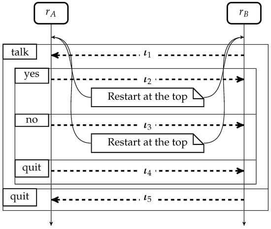
The global type of the $\mathrm{phoneA}$ session from Example 1 is:

$${\mathrm{G}}_1=\mu \mathrm{t}.{\mathrm{r}}_{\mathrm{B}}\to {\mathrm{r}}_{\mathrm{A}}:\left\{\begin{array}{c}{\iota }_1:\mathrm{talk}\left(\mathrm{string}\right).{\mathrm{r}}_{\mathrm{A}}\to {\mathrm{r}}_{\mathrm{B}}:\left\{\begin{array}{c}{\iota }_2:\mathrm{yes}(\mathrm{string}).\mathrm{t},\hfill \\ {\iota }_3:\mathrm{no}(\mathrm{string}).\mathrm{t},\hfill \\ {\iota }_4:\mathrm{quit}\left(\mathrm{string}\right).\mathsf{end}\hfill \end{array}\right\},\hfill \\ {\iota }_5:\mathrm{quit}\left(\mathrm{string}\right).\mathsf{end}\hfill \end{array}\right\}.$$

If ${\iota }_5=[0.95,1]$, it means that $\mathrm{Bob}$ (the person responsible for conducting the poll) is more likely to quit than to finish the poll (as intended). However, if we want a minimal chance for $\mathrm{Bob}$ to stop the polling, this can be done by imposing ${\iota }_5=[0,0.1]$.

The global type of this example can be presented as a sequence diagram (see Figure 2).

In the global type $r_1\to r_2:{\{{\iota }_i:l_i\left(S_i\right).G_i\}}_{i\in I}$, one should not assign arbitrarily the bounds of the probability interval ${\iota }_i=[d_{1i};d_{2i}]$ for $i\in I$, but must instead adhere to certain constraints [25].

Definition 1.

Consider a set of probability intervals ${\left\{{\iota }_i\right\}}_{i\in I}$ of the form ${\iota }_i=[d_{1i};d_{2i}]$.

The set ${\left\{{\iota }_i\right\}}_{i\in I}$ is called proper if

$${\sum }_{i\in I}{d}_{1i}\le 1\le {\sum }_{i\in I}{d}_{2i},$$

while the set ${\left\{{\iota }_i\right\}}_{i\in I}$ is called reachable if for all $i\in I$ it holds that

$$\left({\sum }_{i\ne j}{d}_{1j}\right)+d_{2i}\le 1\le \left({\sum }_{i\ne j}{d}_{2j}\right)+d_{1i}.$$

Example 4.

Consider the set of probability intervals ${\left\{{\iota }_{\mathrm{i}}\right\}}_{\mathrm{i}\in \{1,2\}}$, where ${\iota }_1={\iota }_2=[0.4;0.49]$. Note that ${\left\{{\iota }_{\mathrm{i}}\right\}}_{\mathrm{i}\in \{1,2\}}$ is not proper (since $1\cancel{\le }0.49+0.49=0.98$). This means that if we choose any ${\mathrm{p}}_1\in {\iota }_1$, there is no ${\mathrm{p}}_2\in {\iota }_2$ such that ${\sum }_{\mathrm{i}\in \{1,2\}}{\mathrm{p}}_{\mathrm{i}}=1$. Thus, by defining a set to be proper, we avoid a situation in which we cannot choose a probability from each probability interval such that the sum of the chosen probabilities is 1.

If we modify the intervals with just $0.1$ at the upper part, then the set of probability intervals ${\left\{{\iota }_{\mathrm{i}}\right\}}_{\mathrm{i}\in \{1,2\}}$, where ${\iota }_1={\iota }_2=[0.4;0.59]$, is proper (since $0.4+0.4=0.8\le 1\le 0.59+0.59=1.08$). This is due to the fact that there exist at least a pair, e.g., ${\mathrm{p}}_1=0.45\in {\iota }_1$ and ${\mathrm{p}}_2=0.55\in {\iota }_2$, such that their sum is 1. However, since $1\cancel{\le }0.4+0.59=0.99$, this set is not reachable, meaning that it is not the case that for any ${\mathrm{p}}_1\in {\iota }_1$, there exists a ${\mathrm{p}}_2\in \iota$ such that their sum is 1. For example, if ${\mathrm{p}}_1=0.4$ there is no ${\mathrm{p}}_2=0.6\in {\iota }_2$ such that their sum is 1.

Defining a probability interval as proper and reachable prevents scenarios in which for all $i\in I$ there does not exist $p_i\in {\iota }_i$ such that ${\sum }_{i\in I}{p}_i=1$.

The local types $T,T_i$ shown in

Table 4. Local types of the session typing.

Local	T	$::=$	$r{\oplus }_{i\in I}{\iota }_i:!l_i\langle S_i\rangle .T_i$ $|\hspace{1em}r{\&}_{i\in I}?l_i\left(S_i\right).T_i$ $|\hspace{1em}\mu t.T$ | t | end
Sorts	S	$::=$	$\mathit{nat}\mid \mathit{bool}\mid \dots$

describe the local behavior of processes, and also serve as a link between the global types and the processes of our calculus.

The selection type $r{\oplus }_{i\in I}{\iota }_i:!l_i\langle S_i\rangle .T_i$ represents a channel that can choose a label $l_i$ with a probability belonging to the probability interval ${\iota }_i$ (for any $i\in I$), send it to r along with a variable of type $S_i$ and then proceed as $T_i$. The branching type $r{\&}_{i\in I}?l_i\left(S_i\right).T_i$ represents a channel that can receive a label $l_i$ from role r (for some $i\in I$, chosen by r), along with a variable of type $S_i$ and then proceed as $T_i$. In both selection and branching types, the labels $l_i$ are distinct and their order does not matter. The recursive type $\mu t.T$ and type variable t model infinite behaviors. Type end represents a terminated channel (and it is often omitted). The base types $S,S_0,S_1,\dots$ can include types such as $\mathit{bool}$, $\mathit{int}$, and others.

We define the projection of a global type onto its corresponding local types.

Definition 2.

The projection $G\upharpoonright r$ for a participant with role r appearing in a global type G is inductively defined as:

• $(r_1\to r_2:{\{{\iota }_i:l_i\left(S_i\right).G_i\}}_{i\in I})\upharpoonright r=$$\left\{\begin{array}{cc}{r}_2{\oplus }_{i\in I}{\iota }_i:!l_i\langle S_i\rangle .(G_i\upharpoonright r)\hfill & if r=r_1\ne r_2\hfill \\ r_1{\&}_{i\in I}?l_i\left(S_i\right).(G_i\upharpoonright r)\hfill & if r=r_2\ne r_1\hfill \\ G_1\upharpoonright r\hfill & if r_1\ne r\ne r_2,\hfill \\ & \forall i,j\in I,G_i\upharpoonright r=G_j\upharpoonright r\ne t^{\prime }(\forall t^{\prime })\hfill \end{array}\right.$;
• $(\mu t.G)\upharpoonright r=\left\{\begin{array}{cc}\mu t.(G\upharpoonright r)\hfill & if G\upharpoonright r\ne t^{\prime }(\forall t^{\prime })\hfill \\ \mathsf{end}\hfill \end{array}\right.$;
• $t\upharpoonright r=t$;
• $\mathsf{end}\upharpoonright r=\mathsf{end}$.

If none of the conditions are satisfied, the projection is undefined.

Example 5.

Consider the global type ${\mathrm{G}}_1$ of Example 3:

$${\mathrm{G}}_1=\mu \mathrm{t}.{\mathrm{r}}_{\mathrm{B}}\to {\mathrm{r}}_{\mathrm{A}}:\left\{\begin{array}{c}{\iota }_1:\mathrm{talk}\left(\mathrm{string}\right).{\mathrm{r}}_{\mathrm{A}}\to {\mathrm{r}}_{\mathrm{B}}:\left\{\begin{array}{c}{\iota }_2:\mathrm{yes}(\mathrm{string}).\mathrm{t},\hfill \\ {\iota }_3:\mathrm{no}(\mathrm{string}).\mathrm{t},\hfill \\ {\iota }_4:\mathrm{quit}\left(\mathrm{string}\right).\mathsf{end}\hfill \end{array}\right\},\hfill \\ {\iota }_5:\mathrm{quit}\left(\mathrm{string}\right).\mathsf{end}\hfill \end{array}\right\}.$$

The local types obtained from the global type $G_1$ by using the projection of Definition 2 for each of the two roles are as follows:

$${\mathrm{T}}_{\mathrm{A}}={\mathrm{G}}_1\upharpoonright r_A=\mu \mathrm{t}.{\mathrm{r}}_{\mathrm{B}}\&\left\{\begin{array}{c}?\mathrm{talk}\left(\mathrm{string}\right).{\mathrm{T}}_{\mathrm{A}}^{\prime },\hfill \\ ?\mathrm{quit}\left(\mathrm{string}\right).\mathsf{end}\hfill \end{array}\right\}, \mathit{where}{\mathrm{T}}_{\mathrm{A}}^{\prime }={\mathrm{r}}_{\mathrm{B}}\oplus \left\{\begin{array}{c}{\iota }_2:!\mathrm{yes}(\mathrm{string}).\mathrm{t},\hfill \\ {\iota }_3:!\mathrm{no}(\mathrm{string}).\mathrm{t},\hfill \\ {\iota }_4:!\mathrm{quit}\left(\mathrm{string}\right).\mathsf{end}\hfill \end{array}\right\}$$

$${\mathrm{T}}_{\mathrm{B}}={\mathrm{G}}_1\upharpoonright r_B=\mu \mathrm{t}.{\mathrm{r}}_{\mathrm{A}}\oplus \left\{\begin{array}{c}{\iota }_1:!\mathrm{talk}\left(\mathrm{string}\right).{\mathrm{T}}_{\mathrm{B}}^{\prime },\hfill \\ {\iota }_5:!\mathrm{quit}\left(\mathrm{string}\right).\mathsf{end}\hfill \end{array}\right\}, \mathit{where}{\mathrm{T}}_{\mathrm{B}}^{\prime }={\mathrm{r}}_{\mathrm{A}}\&\left\{\begin{array}{c}?\mathrm{yes}(\mathrm{string}).\mathrm{t},\hfill \\ ?\mathrm{no}(\mathrm{string}).\mathrm{t},\hfill \\ ?\mathrm{quit}\left(\mathrm{string}\right).\mathsf{end}\hfill \end{array}\right\}$$

In order to state subject reduction (a property that ensures that the type of a process is preserved during its evaluation), we need to formalize how global types are modified when multiparty sessions evolve.

Definition 3

(Global type consumption). If G is a global type, then $G\stackrel{r_1\to r_2:\{\iota :l\}}{\to }{G}^{\prime }$ denoting that G is reduced by consumption of a communication between roles $r_1$ and $r_2$ is defined inductively as follows:

• $r_1\to r_2:{\{{\iota }_i:l_i\left(S_i\right).G_i\}}_{i\in I}\stackrel{r_1\to r_2:\{\iota :l\}}{\to }{G}_k$ if $\exists k\in I$ s.t. $l=l_k$, $\iota ={\iota }_k$;
• $r_3\to r_4:{\{{\iota }_i:l_i\left(S_i\right).G_i\}}_{i\in I}\stackrel{r_1\to r_2:\{\iota :l\}}{\to }{r}_3\to r_4:{\{{\iota }_i:l_i\left(S_i\right).G_i^{\prime }\}}_{i\in I}$ if $\{r_1,r_2\}\cap \{r_3,r_4\}=\varnothing$ and $\forall i.G_i\stackrel{r_1\to r_2:\{\iota :l\}}{\to }{G}_i^{\prime }$.

Example 6.

Consider the global type ${\mathrm{G}}_1$ of Example 3:

$${\mathrm{G}}_1=\mu \mathrm{t}.{\mathrm{r}}_{\mathrm{B}}\to {\mathrm{r}}_{\mathrm{A}}:\left\{\begin{array}{c}{\iota }_1:\mathrm{talk}\left(\mathrm{string}\right).{\mathrm{r}}_{\mathrm{A}}\to {\mathrm{r}}_{\mathrm{B}}:\left\{\begin{array}{c}{\iota }_2:\mathrm{yes}(\mathrm{string}).\mathrm{t},\hfill \\ {\iota }_3:\mathrm{no}(\mathrm{string}).\mathrm{t},\hfill \\ {\iota }_4:\mathrm{quit}\left(\mathrm{string}\right).\mathsf{end}\hfill \end{array}\right\},\hfill \\ {\iota }_5:\mathrm{quit}\left(\mathrm{string}\right).\mathsf{end}\hfill \end{array}\right\}.$$

Since we take the equi-recursive viewpoint [27], i.e., we identify $\mu \mathrm{t}.\mathrm{G}$ with $\mathrm{G}\left\{\mu \mathrm{t}.\mathrm{G}/\mathrm{t}\right\}$, it follows that ${\mathrm{G}}_1$ can be written as:

$${\mathrm{G}}_1={\mathrm{r}}_{\mathrm{B}}\to {\mathrm{r}}_{\mathrm{A}}:\left\{\begin{array}{c}{\iota }_1:\mathrm{talk}\left(\mathrm{string}\right).{\mathrm{r}}_{\mathrm{A}}\to {\mathrm{r}}_{\mathrm{B}}:\left\{\begin{array}{c}{\iota }_2:\mathrm{yes}(\mathrm{string}).{\mathrm{G}}_1,\hfill \\ {\iota }_3:\mathrm{no}(\mathrm{string}).{\mathrm{G}}_1,\hfill \\ {\iota }_4:\mathrm{quit}\left(\mathrm{string}\right).\mathsf{end}\hfill \end{array}\right\},\hfill \\ {\iota }_5:\mathrm{quit}\left(\mathrm{string}\right).\mathsf{end}\hfill \end{array}\right\}.$$

Then, by Definition 3, type ${\mathrm{G}}_1$ can be reduced as follows:

$${\mathrm{G}}_1\stackrel{{\mathrm{r}}_{\mathrm{B}}\to {\mathrm{r}}_{\mathrm{A}}:\{{\iota }_1:\mathrm{talk}\}}{\to }{\mathrm{G}}_1^{\prime },\mathit{where}{\mathrm{G}}_1^{\prime }={\mathrm{r}}_{\mathrm{A}}\to {\mathrm{r}}_{\mathrm{B}}:\left\{\begin{array}{c}{\iota }_2:\mathrm{yes}(\mathrm{string}).{\mathrm{G}}_1,\hfill \\ {\iota }_3:\mathrm{no}(\mathrm{string}).{\mathrm{G}}_1,\hfill \\ {\iota }_4:\mathrm{quit}\left(\mathrm{string}\right).\mathsf{end}\hfill \end{array}\right\}.$$

Following the methodology presented in [1], we design a distributed system in terms of global types which is then implemented as a set of processes that adhere to local types, local types derived as projections of the global types.

Given a global type G, in what follows $\mathit{pid}\left(G\right)$ denotes the set of participants in G.

Definition 4.

A global type G is said to be well-formed if:

• for all $r\in \mathit{pid}\left(G\right)$, the projection $G\upharpoonright r$ is defined;
• in all its subterms of the form $r_1\to r_2:{\{{\iota }_i:l_i\left(S_i\right).G_i\}}_{i\in I}$, the set of intervals ${\left\{{\iota }_i\right\}}_{i\in I}$ is proper and reachable.

Example 7.

Consider the global type ${\mathrm{G}}_1$ of Example 3:

$${\mathrm{G}}_1=\mu \mathrm{t}.{\mathrm{r}}_{\mathrm{B}}\to {\mathrm{r}}_{\mathrm{A}}:\left\{\begin{array}{c}{\iota }_1:\mathrm{talk}\left(\mathrm{string}\right).{\mathrm{r}}_{\mathrm{A}}\to {\mathrm{r}}_{\mathrm{B}}:\left\{\begin{array}{c}{\iota }_2:\mathrm{yes}(\mathrm{string}).\mathrm{t},\hfill \\ {\iota }_3:\mathrm{no}(\mathrm{string}).\mathrm{t},\hfill \\ {\iota }_4:\mathrm{quit}\left(\mathrm{string}\right).\mathsf{end}\hfill \end{array}\right\},\hfill \\ {\iota }_5:\mathrm{quit}\left(\mathrm{string}\right).\mathsf{end}\hfill \end{array}\right\},$$

in which for all $\mathrm{i}\in \{1,\dots 4\}$ it holds that ${\iota }_{\mathrm{i}}=[0,1]$ and also ${\iota }_5=[0.95,1]$. As seen in Example 5, ${\mathrm{G}}_1\upharpoonright \mathrm{r}$ is defined for all roles. Moreover, since $0+0+0=0\le 1\le 1+1+1=3$, the set ${\left\{{\iota }_{\mathrm{i}}\right\}}_{\mathrm{i}\in \{2,3,4\}}$ is proper (there exist at least a probability in each probability interval such that their sum is 1: e.g., ${\mathrm{p}}_2=0\in {\iota }_2$, ${\mathrm{p}}_3=0\in {\iota }_3$ and ${\mathrm{p}}_3=1\in {\iota }_4$) and since $0+0+1=1\le 1\le 1+1+0=2$, then the set ${\left\{{\iota }_{\mathrm{i}}\right\}}_{\mathrm{i}\in \{2,3,4\}}$ is reachable (for all $\mathrm{i}\in \{2,3,4\}$ by choosing ${\mathrm{p}}_{\mathrm{i}}\in {\iota }_{\mathrm{i}}$ there exists $\mathrm{j}\ne \mathrm{k}\in \{2,3,4\}\setminus \mathrm{i}$ such that ${\mathrm{p}}_{\mathrm{j}}\in {\iota }_{\mathrm{j}}$, ${\mathrm{p}}_{\mathrm{k}}\in {\iota }_{\mathrm{k}}$ and ${\mathrm{p}}_{\mathrm{i}}+{\mathrm{p}}_{\mathrm{j}}+{\mathrm{p}}_{\mathrm{k}}=1$).

Also, since $0+0.95=0.95\le 1+1=2$, the set ${\left\{{\iota }_{\mathrm{i}}\right\}}_{\mathrm{i}\in \{1,5\}}$ is proper (there exist at least a probability in each probability interval such that their sum is 1: e.g., ${\mathrm{p}}_1=0.05\in {\iota }_1$ and ${\mathrm{p}}_5=0.95\in {\iota }_5$), while, since $1+0.95\cancel{\le }1$, the set ${\left\{{\iota }_{\mathrm{i}}\right\}}_{\mathrm{i}\in \{1,5\}}$ is not reachable (for ${\mathrm{p}}_1=0.5\in {\iota }_1$, there does not exists ${\mathrm{p}}_5=0.5\in {\iota }_5$ such that ${\mathrm{p}}_1+{\mathrm{p}}_5=1$).

Thus, having a proper and reachable set of probabilities is often a desirable requirement; it can serve as a sanity check for a specification.

4. Interval Probability for Multiparty Session Types

4.1. Typing System

We present how the notions defined in Section 2 and Section 3 (namely, the probabilistic processes and the global/local types using probability intervals) are connected. To achieve this, we introduce sortings $\mathsf{\Gamma }$ and typings $\Delta$, specifically

$$\mathsf{\Gamma }::=\varnothing \mid \mathsf{\Gamma },x:S\mid \mathsf{\Gamma },X:\tilde{S}\tilde{T}\hspace{1em}\mathrm{and}\hspace{1em}\Delta ::=\varnothing \mid \Delta ,s\left[r\right]:T.$$

The typing system uses a map from shared names to their sorts $(S,S^{\prime },\dots )$. A sorting $(\mathsf{\Gamma },{\mathsf{\Gamma }}^{\prime },\dots )$ is a finite map that associates names with sorts, and process variables with sequences of sorts and types. A typing $(\Delta ,{\Delta }^{\prime },\dots )$ tracks the usage of session channels. The disjoint union $\Delta ,{\Delta }^{\prime }$ of two typings $\Delta$ and ${\Delta }^{\prime }$ is defined only if the sets of channels contained in the domains of these two typings are distinct. In what follows, we denote by $\mathcal{S}$ and $\mathcal{T}$ the set of all sortings and typings, respectively.

The dynamics of the types of the interacting processes is defined as in [1] by a labelled type reduction relation ${\Rightarrow }_{\iota }$ on typing $\Delta$ that respects the following rules:

• $s\left[r_1\right]:r_2{\oplus }_{i\in I}{\iota }_i:!l_i\langle S_i\rangle .T_i$,$s\left[r_2\right]:r_1{\&}_{i\in I}?l_i\left(S_i\right).T_i^{\prime }$${\Rightarrow }_{{\iota }_k}$$s\left[r_1\right]:T_k$,$s\left[r_2\right]:T_k^{\prime }$ for $k\in I$;
• $s\left[r\right]:\mu t.T$${\Rightarrow }_1$$s\left[r\right]:T\{\mu t.T/t\}$;
• $\Delta ,{\Delta }^{\prime }{\Rightarrow }_{\iota }\Delta ,{\Delta }^{\prime \prime }$ whenever ${\Delta }^{\prime }{\Rightarrow }_{\iota }{\Delta }^{\prime \prime }$.

The first rule indicates two participants with roles $r_1$ and $r_2$ that use a label $l_k$ to communicate on the session channel s a value of type $S_k$. Notice that the reduction arrow is decorated with the probability interval of the sending type; this would be useful when proving type preservation under evolution. The second rule describes the unfolding of local types with probability interval $[1,1]$, while the third rule refers to the composition of two typings when only one of them is evolving.

We describe that a typing $\Delta$ is safe as in [28]; this property is independent of the probability intervals present in $\Delta$.

Definition 5.

φ is a safety property of typing contexts if and only if:

• $\phi (\Delta ,s\left[r_1\right]:r_2{\oplus }_{i\in I}{\iota }_i:!l_i\langle S_i\rangle .T_i$, $s\left[r_2\right]:r_1{\&}_{j\in J}?l_j\left(S_j\right).T_j^{\prime })$ implies $I\subseteq J$;
• $\phi (\Delta ,s[p]:\mu t.T)$ implies $\phi (\Delta ,s[p]:T\{\mu t.T/t\left\}\right)$;
• $\phi (\Delta )$ and $\Delta {\Rightarrow }_{\iota }{\Delta }^{\prime }$ implies $\phi \left({\Delta }^{\prime }\right)$.

We say Δ is safe if $\phi (\Delta )$ for some safety property φ. The fact that Δ is safe is denoted by $\mathit{safe}(\Delta )$.

If the safety property $\phi$ is not explicitly instantiated, then, as in [28], we consider $\phi =\mathit{safe}$ (i.e., the largest safety property, cf. Definition 5).

Example 8.

Consider the local types ${\mathrm{T}}_{\mathrm{A}}$ and ${\mathrm{T}}_{\mathrm{B}}$ from Example 5 and the typing:

$$\Delta =\mathrm{phoneA}\left[{\mathrm{r}}_{\mathrm{A}}\right]:{\mathrm{T}}_{\mathrm{A}},\mathrm{phoneA}\left[{\mathrm{r}}_{\mathrm{B}}\right]:{\mathrm{T}}_{\mathrm{B}},\mathrm{imA}\left[{\mathrm{r}}_{\mathrm{A}}\right]:{\mathrm{T}}_{\mathrm{A}},\mathrm{imA}\left[{\mathrm{r}}_{\mathrm{B}}\right]:{\mathrm{T}}_{\mathrm{B}}$$

We can verify that $\mathit{safe}(\Delta )$ holds by checking its reductions.

Note that the safety of disjoint unions of typings is preserved by each of these disjoint typings.

Proposition 1.

If $\mathit{safe}(\Delta ,{\Delta }^{\prime })$, then $\mathit{safe}(\Delta )$.

Proof. 

By contradiction, assume that it is not the case that $\mathit{safe}(\Delta )$ holds. Then, by Definition 5 (last clause), there is ${\Delta }^{\prime \prime }$ such that $\Delta {\Rightarrow }_{\iota }{\Delta }^{\prime \prime }$, and ${\Delta }^{\prime \prime }$ violates the first clause of Definition 5 (possibly after applying the second clause if some unfolding is needed). However, by the last clause of the definition of the labelled type reduction relation ${\Rightarrow }_{\iota }$, it holds that $\Delta ,{\Delta }^{\prime }{\Rightarrow }_{\iota }{\Delta }^{\prime \prime },{\Delta }^{\prime }$ and it is not the case that $\mathit{safe}({\Delta }^{\prime \prime },{\Delta }^{\prime })$ holds. This means the disjoint union $\Delta ,{\Delta }^{\prime }$ violates the first clause of Definition 5 and therefore it is not the case that $\mathit{safe}(\Delta ,{\Delta }^{\prime })$ holds, which represents a contradiction. Thus, we conclude that $\mathit{safe}(\Delta )$ holds. □

Example 9.

Consider from Example 8 the typing:

$$\Delta =\mathrm{phoneA}\left[{\mathrm{r}}_{\mathrm{A}}\right]:{\mathrm{T}}_{\mathrm{A}},\mathrm{phoneA}\left[{\mathrm{r}}_{\mathrm{B}}\right]:{\mathrm{T}}_{\mathrm{B}},\mathrm{imA}\left[{\mathrm{r}}_{\mathrm{A}}\right]:{\mathrm{T}}_{\mathrm{A}},\mathrm{imA}\left[{\mathrm{r}}_{\mathrm{B}}\right]:{\mathrm{T}}_{\mathrm{B}}.$$

Then Δ can be written as a disjoint union of two typings, namely $\Delta ={\Delta }_1,{\Delta }_2$, where ${\Delta }_1=\mathrm{phoneA}\left[{\mathrm{r}}_{\mathrm{A}}\right]:{\mathrm{T}}_{\mathrm{A}},\mathrm{phoneA}\left[{\mathrm{r}}_{\mathrm{B}}\right]:{\mathrm{T}}_{\mathrm{B}}$ and ${\Delta }_2=\mathrm{imA}\left[{\mathrm{r}}_{\mathrm{A}}\right]:{\mathrm{T}}_{\mathrm{A}},\mathrm{imA}\left[{\mathrm{r}}_{\mathrm{B}}\right]:{\mathrm{T}}_{\mathrm{B}}$. From Example 8, $\mathit{safe}(\Delta )$ holds; according to Proposition 1, $\mathit{safe}\left({\Delta }_1\right)$ and $\mathit{safe}\left({\Delta }_2\right)$ also hold.

In order to establish a connection between the global types G and typings $\Delta$, being inspired by [29], we define the full projection of a global type as a typing. This full projection is useful in defining the typing system and proving the subject reduction.

Definition 6

(Full projection). If G is the global type of a session s such that $\mathit{pid}\left(G\right)=I$ and $\mathit{safe}\left({\{s\left[r_i\right]:T_i\}}_{i\in I}\right)$ where for all $i\in I$ it holds that $G\upharpoonright r_i$=$T_i$, then the full projection of G on s is given by $〚G{〛}_s={\{s\left[r_i\right]:T_i\}}_{i\in I}$.

Example 10.

Consider the global type ${\mathrm{G}}_1$ of Example 3, the local types ${\mathrm{T}}_{\mathrm{A}}$ and ${\mathrm{T}}_{\mathrm{B}}$ obtained from ${\mathrm{G}}_1$ in Example 5 and the safe typing ${\Delta }_1=\mathrm{phoneA}\left[{\mathrm{r}}_{\mathrm{A}}\right]:{\mathrm{T}}_{\mathrm{A}},\mathrm{phoneA}\left[{\mathrm{r}}_{\mathrm{B}}\right]:{\mathrm{T}}_{\mathrm{B}}$ obtained in Example 9. Then, by Definition 6, the full projection of ${\mathrm{G}}_1$ on $\mathrm{phoneA}$ is $〚{\mathrm{G}}_1{〛}_{\mathrm{phoneA}}={\Delta }_1$.

The connection between the evolution of global types and that of the corresponding typings can be expressed as in the following result.

Proposition 2.

If $\Delta {\Rightarrow }_{\iota }{\Delta }^{\prime }$ and $\mathit{safe}(\Delta )$, then there exist $s,r_1,r_2,l,G,G^{\prime }$ such that $\Delta ={\Delta }^{\prime \prime },〚G{〛}_s$ and ${\Delta }^{\prime }={\Delta }^{\prime \prime },〚G^{\prime }{〛}_s$, where $G\stackrel{r_1\to r_2:\{\iota :l\}}{\to }{G}^{\prime }$.

Proof. 

Since $\Delta {\Rightarrow }_{\iota }{\Delta }^{\prime }$ and $\mathit{safe}(\Delta )$, then the associated redex is in ${\Delta }_s={\{s\left[r_i\right]:T_i\}}_{i\in I}$, where $\Delta ={\Delta }^{\prime \prime },{\Delta }_s$. Due to Proposition 1, it holds that $\mathit{safe}\left({\Delta }_s\right)$, and thus we can write ${\Delta }_s$ as $〚G{〛}_s$ for some well-formed global type G. By taking the preimage of the associated redex in $〚G{〛}_s$, reducing G by $G\stackrel{r_1\to r_2:\{\iota :l\}}{\to }{G}^{\prime }$ corresponds to eliminating its preimage from G to obtain $G^{\prime }$, whose projection $〚G^{\prime }{〛}_s$ precisely gives the result of reducing $〚G{〛}_s={\Delta }_s$ to $〚G^{\prime }{〛}_s={\Delta }_s^{\prime }$, and thus ${\Delta }^{\prime }={\Delta }^{\prime \prime },〚G^{\prime }{〛}_s$. □

Example 11.

Consider the global type ${\mathrm{G}}_1$ of Example 3, the local types ${\mathrm{T}}_{\mathrm{A}}$ and ${\mathrm{T}}_{\mathrm{B}}$ obtained from ${\mathrm{G}}_1$ in Example 5 and the safe typing ${\Delta }_1=\mathrm{phoneA}\left[{\mathrm{r}}_{\mathrm{A}}\right]:{\mathrm{T}}_{\mathrm{A}},\mathrm{phoneA}\left[{\mathrm{r}}_{\mathrm{B}}\right]:{\mathrm{T}}_{\mathrm{B}}$ obtained in Example 9 such that $〚{\mathrm{G}}_1{〛}_{\mathrm{phoneA}}={\Delta }_1$ as obtained in Example 10.

By using the labelled type reduction relation ${\Rightarrow }_{\iota }$ on typing ${\Delta }_1$, we have that ${\Delta }_1{\Rightarrow }_{{\iota }_1}{\Delta }_1^{\prime }$, where ${\Delta }_1^{\prime }=\mathrm{phoneA}\left[{\mathrm{r}}_{\mathrm{A}}\right]:{\mathrm{T}}_{\mathrm{A}}^{\prime },\mathrm{phoneA}\left[{\mathrm{r}}_{\mathrm{B}}\right]:{\mathrm{T}}_{\mathrm{B}}^{\prime }$. Since $\mathit{safe}\left({\Delta }_1\right)$ holds from Exercise 9, then by Definition 5 also $\mathit{safe}\left({\Delta }_1^{\prime }\right)$ holds. From Example 6, it holds that ${\mathrm{G}}_1\stackrel{{\mathrm{r}}_{\mathrm{B}}\to {\mathrm{r}}_{\mathrm{A}}:\{{\iota }_1:\mathrm{talk}\}}{\to }{\mathrm{G}}_1^{\prime }$. By Definition 2, the local types ${\mathrm{T}}_{\mathrm{A}}^{\prime }={\mathrm{G}}_1^{\prime }\upharpoonright r_A$ and ${\mathrm{T}}_{\mathrm{B}}^{\prime }={\mathrm{G}}_1^{\prime }\upharpoonright r_B$ are obtained from ${\mathrm{G}}_1^{\prime }$. Thus, by Definition 6, the full projection ${\mathrm{G}}_1^{\prime }$ on $\mathrm{phoneA}$ is $〚{\mathrm{G}}_1^{\prime }{〛}_{\mathrm{phoneA}}={\Delta }_1^{\prime }$, and so the result of Proposition 2 holds.

The type-assignment system for processes is given in

Table 5. Typing system for processes in probabilistic multiparty sessions.

$\mathsf{\Gamma },x:S⊢x:S$    $\mathsf{\Gamma }⊢v:S$	(TVar), (TVal)
${\displaystyle \frac{\forall i.\mathsf{\Gamma }⊢v_i:S_i\forall i.\mathsf{\Gamma }⊢P_i⊳\Delta ,c:T_i{p}_i\in {\iota }_i}{\mathsf{\Gamma }⊢c\left[r\right]{\oplus }_{i\in I}\langle p_i:l_i\left(v_i\right).P_i\rangle ⊳\Delta ,c:r{\oplus }_{i\in I}{\iota }_i:!l_i\langle S_i\rangle .T_i}}$	(TSelect)
${\displaystyle \frac{\forall i.\mathsf{\Gamma },x_i:S_i⊢P_i⊳\Delta ,c:T_i,I\subseteq J}{\mathsf{\Gamma }⊢c\left[r\right]{\&}_{j\in J}\{l_j\left(x_j\right).P_j\}⊳\Delta ,c:r{\&}_{i\in I}?l_i\left(S_i\right).T_i}}$	(TBranch)
${\displaystyle \frac{\Delta \mathsf{end}\mathit{only}}{\mathsf{\Gamma }⊢\mathbf{0}⊳\Delta }}$       ${\displaystyle \frac{\mathsf{\Gamma }⊢P⊳\Delta \mathsf{\Gamma }⊢Q⊳{\Delta }^{\prime }}{\mathsf{\Gamma }⊢P\mid Q⊳\Delta ,{\Delta }^{\prime }}}$	(TEnd), (TConc)
${\displaystyle \frac{\mathsf{\Gamma }⊢P⊳\Delta ,〚G{〛}_s}{\mathsf{\Gamma }⊢\left(\nu s\right)P⊳\Delta }}$	(TRes)
${\displaystyle \frac{\begin{array}{c}\mathsf{\Gamma },x:\tilde{S},X:\tilde{S}{T}_1\dots T_n⊢P⊳c_1:T_1,\dots ,c_n:T_n\\ \mathsf{\Gamma },X:\tilde{S}{T}_1\dots T_n⊢Q⊳\Delta \end{array}}{\mathsf{\Gamma }⊢\mathsf{def}X(\tilde{x}{c}_1\dots c_n)=P\mathsf{in}Q⊳\Delta }}$	(TDef)
${\displaystyle \frac{\mathsf{\Gamma }⊢\tilde{v}:\tilde{S}\Delta \mathsf{end}\mathit{only}}{\mathsf{\Gamma },X:\tilde{S}{T}_1\dots T_n⊢X(\tilde{v}{c}_1\dots c_n)⊳\Delta ,c_1:T_1,\dots ,c_n:T_n}}$	(TCall)

. We use the judgement $\mathsf{\Gamma }⊢P⊳\Delta$ saying that “under the sorting $\mathsf{\Gamma }$, process P has typing $\Delta$”. Actually, we have two types of rules: some rules using only $\mathsf{\Gamma }$ and others using both $\mathsf{\Gamma }$ and $\Delta$. We use the rules (TVar) and (TVal) for typing variables and values (using only the sorting $\mathsf{\Gamma }$). (TSelect) and (TBranch) are the rules for typing selection and branching, respectively. Just like in [30], the (TSelect) rule states that the selection process is well-typed if $c\left[r\right]$ has a compatible selection (branching) type and the continuations $P_i$ (for all $i\in I$) are well-typed with respect to the session types. Since rule (TSelect) types the selection process by using probability intervals, it should verify that the probabilities fall within the corresponding probability interval. Instead, the (TBranch) rule states that the branching process is well-typed if each $c:r$ from the branching type has a compatible branching process and the continuations $P_i$ (for all $i\in I$) are well-typed with respect to the session types; thus, it allows more branches in the process than in the global type, just mimicking the subtyping for session types [31]. Rule (TEnd) is standard; “$\Delta \mathsf{end}\mathit{only}$” means that $\Delta$ contains only end as session types. Rule (TConc) is composed of two processes if their local types are disjoint. (TRes) is the restriction rule for session names, claiming that $\left(\nu s\right)P$ is well-typed in $\mathsf{\Gamma }$; this happens if the full projection $〚G{〛}_s$ of the global type G associated with the session s appears in the typing associated with process P. (TDef) says that a process definition $\mathsf{def}X(\tilde{x}{c}_1\dots c_n)=P\mathsf{in}Q$ is well-typed if both P and Q are well-typed in their typing contexts. Rule (TCall) says that a process call $X(\tilde{v}{c}_1\dots c_n)$ is well-typed if the actual parameters $\tilde{v}{c}_1\dots c_n$ have compatible types with respect to X.

Example 12.

Consider from Example 2 the process

$\mathrm{AB}=\mathsf{def}\mathrm{B}(\mathrm{y},\mathrm{q})={\mathrm{B}}_1\mathsf{in}\mathsf{def}\mathrm{A}\left(\mathrm{y}\right)={\mathrm{A}}_1\mathsf{in}{\mathrm{A}}_1\{\mathrm{phoneA}\left[{\mathrm{r}}_{\mathrm{A}}\right]/\mathrm{y}\})\mid {\mathrm{B}}_1\{\mathrm{PhoneNoA}\left[{\mathrm{r}}_{\mathrm{B}}\right]/\mathrm{y},{\mathrm{q}}_1/\mathrm{q}\}$, and the safe typing ${\Delta }_1=\mathrm{phoneA}\left[{\mathrm{r}}_{\mathrm{A}}\right]:{\mathrm{T}}_{\mathrm{A}},\mathrm{phoneA}\left[{\mathrm{r}}_{\mathrm{B}}\right]:{\mathrm{T}}_{\mathrm{B}}$ obtained in Example 9.

By using the rules of Table 5, we can type the process $\mathrm{AB}$ with the typing ${\Delta }_1$ and the empty sorting ∅, namely $\varnothing ⊢\mathrm{AB}⊳{\Delta }_1$.

4.2. Behavioral Properties of Typed Processes

We can prove that our probabilistic typing system is sound, meaning that its term-checking rules admit only consistent terms with respect to the structural congruence and operational semantics.

A subject reduction property ensures that the type of an expression is preserved during its evaluation. For proving this property, we need the following substitution, weakening and strengthening results.

Lemma 1.

• (substitution)  If $\mathsf{\Gamma },x:S⊢P⊳\Delta$ and $\mathsf{\Gamma }⊢v:S$ then $\mathsf{\Gamma }⊢P\{v/x\}⊳\Delta$.
• (type weakening) If $\mathsf{\Gamma }⊢P⊳\Delta$ and ${\Delta }^{\prime }$ is only end, then $\mathsf{\Gamma }⊢P⊳\Delta ,{\Delta }^{\prime }$.
• (type strengthening) If $s\left[r\right]\notin \mathit{fc}\left(P\right)$ and $\mathsf{\Gamma }⊢P⊳\Delta ,\left\{s\right[r]:T\}$, then $\mathsf{\Gamma }⊢P⊳\Delta$.
• (sort weakening) If $X\notin dom\left(\mathsf{\Gamma }\right)$ and $\mathsf{\Gamma }⊢P⊳\Delta$, then $\mathsf{\Gamma },X:\tilde{S}\tilde{T}⊢P⊳\Delta$.
• (sort strengthening) If $X\notin fpv\left(P\right)$ and $\mathsf{\Gamma },X:\tilde{S}\tilde{T}⊢P⊳\Delta$, then $\mathsf{\Gamma }⊢P⊳\Delta$.

Proof. 

The proofs are rather standard, by induction on the derivations on the premise, following those presented in [1]. □

The next result states that if under the sorting $\mathsf{\Gamma }$, a process P has typing $\Delta$, then rearranging the process P into process $P^{\prime }$ by using the structural congruence ≡, then the process $P^{\prime }$ is typed using the same sorting $\mathsf{\Gamma }$ and the same typing $\Delta$.

Theorem 1

(Subject equivalence). $\mathsf{\Gamma }⊢P⊳\Delta$ and $P\equiv P^{\prime }$ imply $\mathsf{\Gamma }⊢P^{\prime }⊳\Delta$.

Proof. 

The proof is by induction on ≡, showing that if one side has a typing, then the other side has the same typing. The probability intervals in the involved types remain unchanged because the structural congruence ≡ does not consume or modify the selection processes.

• Case $P\mid \mathbf{0}\equiv P$.
  ⇒ Assume $\mathsf{\Gamma }⊢P\mid \mathbf{0}⊳\Delta$. By inverting the rule (TConc), we obtain $\mathsf{\Gamma }⊢P⊳{\Delta }_1$ and $\mathsf{\Gamma }⊢\mathbf{0}⊳{\Delta }_2$, where ${\Delta }_1,{\Delta }_2=\Delta$. By inverting the rule (TEnd), ${\Delta }_2$ is only end and ${\Delta }_2$ is such that $\mathit{dom}\left({\Delta }_1\right)\cap \mathit{dom}\left({\Delta }_2\right)=\varnothing$. Then, by type weakening, we obtain that $\mathsf{\Gamma }⊢P⊳\Delta$, where $\Delta ={\Delta }_1,{\Delta }_2$.
  ⇐ Assume $\mathsf{\Gamma }⊢P⊳\Delta$. By rule (TEnd), it holds that $\mathsf{\Gamma }⊢\mathbf{0}⊳{\Delta }^{\prime }$, where ${\Delta }^{\prime }$ is only end and $\mathit{dom}(\Delta )\cap \mathit{dom}\left({\Delta }^{\prime }\right)=\varnothing$. By applying the rule (TConc), we obtain $\mathsf{\Gamma }⊢P\mid \mathbf{0}⊳\Delta ,{\Delta }^{\prime }$ and since ${\Delta }^{\prime }=\varnothing$, by type strengthening, we obtain $\mathsf{\Gamma }⊢P\mid \mathbf{0}⊳\Delta$, as required.
• Case $\left(\nu s\right)\mathbf{0}\equiv \mathbf{0}$.
  ⇒ Assume $\mathsf{\Gamma }⊢\left(\nu s\right)\mathbf{0}⊳\Delta$. By inverting the rule (TRes), we obtain $\mathsf{\Gamma }⊢\mathbf{0}⊳\Delta ,〚G{〛}_s$ where $s\notin \Delta$. By inverting the rule (TEnd), $\Delta ,〚G{〛}_s$ is only end, namely $\Delta$ is only end. Using the rule (TEnd), we obtain $\mathsf{\Gamma }⊢\mathbf{0}⊳\Delta$.
  ⇐ Assume $\mathsf{\Gamma }⊢\mathbf{0}⊳\Delta$. By rule (TRes), it holds that $\mathsf{\Gamma }⊢\left(\nu s\right)\mathbf{0}⊳{\Delta }_1$ where $s\notin {\Delta }_1$, $〚G{〛}_s={\{s\left[r_i\right]:\mathsf{end}\}}_{i\in I}$ and $\Delta ={\Delta }_1,〚G{〛}_s$. Then, by type weakening, we obtain that $\mathsf{\Gamma }⊢\left(\nu s\right)\mathbf{0}⊳\Delta$, as required.
• Case $P\mid Q\equiv Q\mid P$
  ⇒ Assume $\mathsf{\Gamma }⊢P\mid Q⊳\Delta$. By inverting the rule (TConc), we obtain $\mathsf{\Gamma }⊢P⊳{\Delta }_1$ and $\mathsf{\Gamma }⊢Q⊳{\Delta }_2$, where ${\Delta }_1,{\Delta }_2=\Delta$. Using the rule (TConc), we obtain $\mathsf{\Gamma }⊢Q\mid P⊳\Delta$.
  ⇐ It follows in a similar way (actually, symmetric to ⇒).
• Case $(P\mid Q)\mid R\equiv P\mid (Q\mid R)$
  ⇒ Assume $\mathsf{\Gamma }⊢(P\mid Q)\mid R⊳\Delta$. By inverting the rule (TConc), we obtain $\mathsf{\Gamma }⊢P⊳{\Delta }_1$, $\mathsf{\Gamma }⊢Q⊳{\Delta }_2$ and $\mathsf{\Gamma }⊢R⊳{\Delta }_3$, where ${\Delta }_1,{\Delta }_2,{\Delta }_3=\Delta$. Using the rule (TConc), we obtain $\mathsf{\Gamma }⊢P\mid (Q\mid R)⊳\Delta$.
  ⇐ It follows in a similar way (actually, symmetric to ⇒).
• Case $\left(\nu s\right)\left(\nu s^{\prime }\right)P\equiv \left(\nu s^{\prime }\right)\left(\nu s\right)P$
  ⇒ Assume $\mathsf{\Gamma }⊢\left(\nu s\right)\left(\nu s^{\prime }\right)P⊳\Delta$. By inverting the rule (TRes) twice, we obtain $\mathsf{\Gamma }⊢P⊳\Delta ,〚G{〛}_s,〚G{〛}_{s^{\prime }}$ where $s\notin \Delta$ and $s^{\prime }\notin \Delta$. Using the rule (TRes), we obtain $\mathsf{\Gamma }⊢\left(\nu s^{\prime }\right)\left(\nu s\right)P⊳\Delta$.
  ⇐ Proof is similar (actually, symmetric to ⇒).
• Case $\left(\nu s\right)P|Q\equiv (\nu s\left)\right(P\left|Q\right)(\mathrm{if}s\notin \mathit{fc}(Q\left)\right)$
  ⇒ Assume $\mathsf{\Gamma }⊢\left(\nu s\right)P|Q⊳\Delta$. Since $s\notin \mathit{fc}\left(\right(\nu s\left)P\right)$ and $s\notin \mathit{fc}\left(Q\right)$, if $s\in \Delta$ (by using type weakening), then $\Delta ={\Delta }^{\prime },{\Delta }^{\prime \prime }$ such that $s\notin {\Delta }^{\prime }$, $s\in {\Delta }^{\prime \prime }$ and ${\Delta }^{\prime \prime }$ is only end. By type strengthening, we obtain $\mathsf{\Gamma }⊢\left(\nu s\right)P|Q⊳{\Delta }^{\prime }$. By inverting the rule (TConc), we obtain $\mathsf{\Gamma }⊢\left(\nu s\right)P⊳{\Delta }_1$ and $\mathsf{\Gamma }⊢Q⊳{\Delta }_2$, where ${\Delta }_1,{\Delta }_2={\Delta }^{\prime }$. By inverting the rule (TRes), we obtain $\mathsf{\Gamma }⊢P⊳{\Delta }_1,〚G{〛}_s$ where $s\notin {\Delta }_1$. Using the rule (TConc), we obtain $\mathsf{\Gamma }⊢P\mid Q⊳{\Delta }_1,〚G{〛}_s,{\Delta }_2$. Since $s\notin \mathit{fc}\left(Q\right)$, it means that ${\Delta }_2$ does not contain types for s; from $\mathsf{\Gamma }⊢P\mid Q⊳{\Delta }_1,{\Delta }_2,〚G{〛}_s$ with $s\notin {\Delta }_1,{\Delta }_2$, by using the rule (TRes) we obtain $\mathsf{\Gamma }⊢\left(\nu s\right)\left(P\right|Q)⊳{\Delta }^{\prime }$, where ${\Delta }_1,{\Delta }_2={\Delta }^{\prime }$. Since ${\Delta }^{\prime \prime }$ is only end, by using type weakening we obtain $\mathsf{\Gamma }⊢\left(\nu s\right)\left(P\right|Q)⊳\Delta$.
  ⇐ Assume $\mathsf{\Gamma }⊢\left(\nu s\right)\left(P\right|Q)⊳\Delta$. By inverting rule (TRes), we obtain $\mathsf{\Gamma }⊢P|Q⊳\Delta ,〚G{〛}_s$, where $s\notin \Delta$. Since $s\notin \mathit{fc}\left(Q\right)$, by inverting the rule (TConc), we obtain $\mathsf{\Gamma }⊢P⊳{\Delta }_1,〚G{〛}_s$ and $\mathsf{\Gamma }⊢Q⊳{\Delta }_2$, where ${\Delta }_1,{\Delta }_2=\Delta$. Using rule (TRes), we obtain $\mathsf{\Gamma }⊢\left(\nu s\right)P⊳{\Delta }_1$. By using rule (TConc), we obtain $\mathsf{\Gamma }⊢\left(\nu s\right)P|Q⊳\Delta$, as required.
• Case $\mathsf{def}D\mathsf{in}\mathbf{0}\equiv \mathbf{0}$
  ⇒ Assume $\mathsf{\Gamma }⊢\mathsf{def}D\mathsf{in}\mathbf{0}⊳\Delta$. By inverting rule (TDef), we obtain $\mathsf{\Gamma },x:\tilde{S},X:\tilde{S}{T}_1\dots T_n⊢P⊳c_1:T_1,\dots ,c_n:T_n$ and $\mathsf{\Gamma },X:\tilde{S}{T}_1\dots T_n⊢\mathbf{0}⊳\Delta$, where $D=\{X(\tilde{x}{c}_1\dots c_n)=P\}$. By inverting rule (TEnd) we obtain that $\Delta$ is only end. Applying rule (TEnd), we obtain $\mathsf{\Gamma }⊢\mathbf{0}⊳\Delta$.
  ⇐ Assume $\mathsf{\Gamma }⊢\mathbf{0}⊳\Delta$. By inverting rule (TEnd), we obtain that $\Delta$ is only end. Applying rule (TEnd), we obtain $\mathsf{\Gamma },X:\tilde{S}{T}_1\dots T_n⊢\mathbf{0}⊳\Delta$. Consider a typable process P such that $\mathsf{\Gamma },x:\tilde{S},X:\tilde{S}{T}_1\dots T_n⊢P⊳c_1:T_1,\dots ,c_n:T_n$. By applying rule (TDef) we obtain that $\mathsf{\Gamma }⊢\mathsf{def}X(\tilde{x}{c}_1\dots c_n)=P\mathsf{in}\mathbf{0}⊳\Delta$, namely $\mathsf{\Gamma }⊢\mathsf{def}D\mathsf{in}\mathbf{0}⊳\Delta$, as required.
• Case $\mathsf{def}D\mathsf{in}\left(\nu s\right)P\equiv \left(\nu s\right)\mathsf{def}D\mathsf{in}P(\mathrm{if}s\notin \mathit{fc}(D\left)\right)$
  ⇒ Assume $\mathsf{\Gamma }⊢\mathsf{def}D\mathsf{in}\left(\nu s\right)P⊳\Delta$. By inverting rule (TDef), we obtain $\mathsf{\Gamma },x:\tilde{S},X:\tilde{S}{T}_1\dots T_n⊢Q⊳c_1:T_1,\dots ,c_n:T_n$ and $\mathsf{\Gamma },X:\tilde{S}{T}_1\dots T_n⊢\left(\nu s\right)P⊳\Delta$, where $D=\{X(\tilde{x}{c}_1\dots c_n)=Q\}$. By inverting the rule (TRes), we obtain $\mathsf{\Gamma }⊢P⊳\Delta ,〚G{〛}_s$ where $s\notin \Delta$. Using rule (TDef), we obtain $\mathsf{\Gamma }⊢\mathsf{def}D\mathsf{in}P⊳\Delta ,〚G{〛}_s$, while using rule (TRes), we obtain $\mathsf{\Gamma }⊢\left(\nu s\right)\mathsf{def}D\mathsf{in}P⊳\Delta$.
  ⇐ Assume $\mathsf{\Gamma }⊢\left(\nu s\right)\mathsf{def}D\mathsf{in}P⊳\Delta$. By inverting rule (TRes), we obtain $\mathsf{\Gamma }⊢\mathsf{def}D\mathsf{in}P⊳\Delta ,〚G{〛}_s$ where $s\notin \Delta$. By inverting rule (TDef), we obtain $\mathsf{\Gamma },x:\tilde{S},X:\tilde{S}{T}_1\dots T_n⊢Q⊳c_1:T_1,\dots ,c_n:T_n$ and $\mathsf{\Gamma },X:\tilde{S}{T}_1\dots T_n⊢P⊳\Delta ,〚G{〛}_s$, where $D=\{X(\tilde{x}{c}_1\dots c_n)=Q\}$. Using rule (TRes), we obtain $\mathsf{\Gamma },X:\tilde{S}{T}_1\dots T_n⊢\left(\nu s\right)P⊳\Delta$. By applying rule (TDef) we obtain that $\mathsf{\Gamma }⊢\mathsf{def}X(\tilde{x}{c}_1\dots c_n)=Q\mathsf{in}\left(\nu s\right)P⊳\Delta$, namely $\mathsf{\Gamma }⊢\mathsf{def}D\mathsf{in}\left(\nu s\right)P⊳\Delta$, as required.
• Case $\mathsf{def}D\mathsf{in}\left(P\right|Q)\equiv (\mathsf{def}D\mathsf{in}P\left)\right|Q\left(\mathrm{if}dpv\right(D)\cap fpv(Q)=\varnothing )$
  ⇒ Assume $\mathsf{\Gamma }⊢\mathsf{def}D\mathsf{in}\left(P\right|Q)⊳\Delta$. By inverting the rule (TDef), we obtain $\mathsf{\Gamma },x:\tilde{S},X:\tilde{S}{T}_1\dots T_n⊢R⊳c_1:T_1,\dots ,c_n:T_n$ and $\mathsf{\Gamma },X:\tilde{S}{T}_1\dots T_n⊢P\mid Q⊳\Delta$, where $D=\{X(\tilde{x}{c}_1\dots c_n)=R\}$. By inverting the rule (TConc), we obtain $\mathsf{\Gamma },X:\tilde{S}{T}_1\dots T_n⊢P⊳{\Delta }_1$ and $\mathsf{\Gamma },X:\tilde{S}{T}_1\dots T_n⊢Q⊳{\Delta }_2$, where ${\Delta }_1,{\Delta }_2=\Delta$. By applying the rule (TDef), we obtain that $\mathsf{\Gamma }⊢\mathsf{def}X(\tilde{x}{c}_1\dots c_n)=R\mathsf{in}P⊳{\Delta }_1$, namely $\mathsf{\Gamma }⊢\mathsf{def}D\mathsf{in}P⊳{\Delta }_1$. Since $dpv\left(D\right)\cap fpv\left(Q\right)=\varnothing$ and $X\in dpv\left(D\right)$, then $X\notin fpv\left(Q\right)$ and so by sort strengthening we obtain $\mathsf{\Gamma }⊢Q⊳{\Delta }_2$. By applying the rule (TConc), we obtain that $\mathsf{\Gamma }⊢\left(\mathsf{def}D\mathsf{in}P\right)\mid Q⊳\Delta$.
  ⇐ Assume $\mathsf{\Gamma }⊢\left(\mathsf{def}D\mathsf{in}P\right)\mid Q⊳\Delta$. By inverting rule (TConc), we obtain $\mathsf{\Gamma }⊢\mathsf{def}D\mathsf{in}P⊳{\Delta }_1$ and $\mathsf{\Gamma }⊢Q⊳{\Delta }_2$, where ${\Delta }_1,{\Delta }_2=\Delta$. By inverting rule (TDef), we obtain $\mathsf{\Gamma },x:\tilde{S},X:\tilde{S}{T}_1\dots T_n⊢R⊳c_1:T_1,\dots ,c_n:T_n$ and $\mathsf{\Gamma },X:\tilde{S}{T}_1\dots T_n⊢P⊳{\Delta }_1$, where $D=\{X(\tilde{x}{c}_1\dots c_n)=R\}$ and $X\notin dom\left(\mathsf{\Gamma }\right)$. Since $X\notin dom\left(\mathsf{\Gamma }\right)$, by sort weakening we obtain $\mathsf{\Gamma },X:\tilde{S}{T}_1\dots T_n⊢Q⊳{\Delta }_2$. By applying rule (TConc), we obtain that $\mathsf{\Gamma },X:\tilde{S}{T}_1\dots T_n⊢P\mid Q⊳\Delta$. By using rule (TDef), we obtain $\mathsf{\Gamma }⊢\mathsf{def}X(\tilde{x}{c}_1\dots c_n)=R\mathsf{in}\left(P\right|Q)⊳\Delta$, namely $\mathsf{\Gamma }⊢\mathsf{def}D\mathsf{in}\left(P\right|Q)⊳\Delta$, as required.
• Case $\mathsf{def}D\mathsf{in}\mathsf{def}{D}^{\prime }\mathsf{in}P\equiv \mathsf{def}{D}^{\prime }\mathsf{in}\mathsf{def}D\mathsf{in}P$$(\mathrm{if}(dpv\left(D\right)\cup fpv\left(D\right))\cap dpv\left(D^{\prime }\right)=(dpv\left(D^{\prime }\right)\cup fpv\left(D^{\prime }\right))\cap dpv\left(D\right)=\varnothing )$
  ⇒ Assume $\mathsf{\Gamma }⊢\mathsf{def}D\mathsf{in}\mathsf{def}{D}^{\prime }\mathsf{in}P⊳\Delta$. By inverting rule (TDef), we obtain $\mathsf{\Gamma },x:\tilde{S},X:\tilde{S}{T}_1\dots T_n⊢R⊳c_1:T_1,\dots ,c_n:T_n$ and $\mathsf{\Gamma },X:\tilde{S}{T}_1\dots T_n⊢\mathsf{def}{D}^{\prime }\mathsf{in}P⊳\Delta$, where $D=\{X(\tilde{x}{c}_1\dots c_n)$$=R\}$. By inverting rule (TDef), we obtain $\mathsf{\Gamma },X:\tilde{S}{T}_1\dots T_n,x^{\prime }:\widetilde{S^{\prime }},X^{\prime }:\widetilde{S^{\prime }}{T}_1^{\prime }\dots$$T_n^{\prime }⊢R^{\prime }⊳c_1^{\prime }:T_1^{\prime },\dots ,c_n^{\prime }:T_n^{\prime }$ and $\mathsf{\Gamma },X:\tilde{S}{T}_1\dots T_n,X^{\prime }:\widetilde{S^{\prime }}{T}_1^{\prime }\dots T_n^{\prime }⊢P⊳\Delta$, where $D^{\prime }=\{X(\widetilde{x^{\prime }}{c}_1^{\prime }\dots c_n^{\prime })=R^{\prime }\}$. Since $(dpv\left(D\right)\cup fpv\left(D\right))\cap dpv\left(D^{\prime }\right)=(dpv\left(D^{\prime }\right)\cup fpv\left(D^{\prime }\right))\cap dpv\left(D\right)=\varnothing$, it means that X and $X^{\prime }$ are different. Applying rule (TDef) twice, we obtain $\mathsf{def}{D}^{\prime }\mathsf{in}\mathsf{def}D\mathsf{in}P$.
  ⇐ It follows in a similar way (actually, symmetric to ⇒).
• $P_0\equiv P_0^{\prime }$ implies $\mathcal{E}\left[P_0\right]\equiv \mathcal{E}\left[P_0^{\prime }\right]$. Let $P\equiv \mathcal{E}\left[P_0\right]$ and $P^{\prime }\equiv \mathcal{E}\left[P_0^{\prime }\right]$.
  The proof is by structural induction on $\mathcal{E}$.

  –

  Case $\mathcal{E}=\left[\right]$. This case is trivial, as $P\equiv P^{\prime }$ is in fact $P_0\equiv P_0^{\prime }$.

  –

  Case $\mathcal{E}=\left(\nu s\right){\mathcal{E}}^{\prime }$. By assumption, $\mathsf{\Gamma }⊢\left(\nu s\right){\mathcal{E}}^{\prime }\left[P_0\right]⊳\Delta$. By inverting the rule (TRes), we obtain that $\mathsf{\Gamma }⊢{\mathcal{E}}^{\prime }\left[P_0\right]⊳\Delta ,〚G{〛}_s$. By structural congruence, $P_0\equiv P_0^{\prime }$ implies $\mathcal{E}\left[P_0\right]\equiv \mathcal{E}\left[P_0^{\prime }\right]$. By induction, $\mathsf{\Gamma }⊢{\mathcal{E}}^{\prime }\left[P_0^{\prime }\right]⊳\Delta ,〚G{〛}_s$. By structural congruence, ${\mathcal{E}}^{\prime }\left[P_0\right]\equiv {\mathcal{E}}^{\prime }\left[P_0^{\prime }\right]$ implies $\mathcal{E}\left[P_0\right]\equiv \mathcal{E}\left[P_0^{\prime }\right]$. By using the rule (TRes), we obtain $\mathsf{\Gamma }⊢\left(\nu s\right){\mathcal{E}}^{\prime }\left[P_0^{\prime }\right]⊳\Delta$, as required.

  –

  Case $\mathcal{E}=\mathsf{def}D\mathsf{in}{\mathcal{E}}^{\prime }$. By assumption, $\mathsf{\Gamma }⊢\mathsf{def}D\mathsf{in}{\mathcal{E}}^{\prime }\left[P_0\right]⊳\Delta$. By inverting rule (TDef), we obtain $\mathsf{\Gamma },x:\tilde{S},X:\tilde{S}{T}_1\dots T_n⊢Q⊳c_1:T_1,\dots ,c_n:T_n$ and $\mathsf{\Gamma },X:\tilde{S}{T}_1\dots T_n⊢{\mathcal{E}}^{\prime }\left[P_0\right]⊳\Delta$, where $D=\{X(\tilde{x}{c}_1\dots c_n)=Q\}$. By structural congruence, $P_0\equiv P_0^{\prime }$ implies $\mathcal{E}\left[P_0\right]\equiv \mathcal{E}\left[P_0^{\prime }\right]$. By induction, $\mathsf{\Gamma },X:\tilde{S}{T}_1\dots T_n⊢{\mathcal{E}}^{\prime }\left[P_0^{\prime }\right]⊳\Delta$. By structural congruence, ${\mathcal{E}}^{\prime }\left[P_0\right]\equiv {\mathcal{E}}^{\prime }\left[P_0^{\prime }\right]$ implies $\mathcal{E}\left[P_0\right]\equiv \mathcal{E}\left[P_0^{\prime }\right]$. By using the rule (TDef), we obtain $\mathsf{\Gamma }⊢\mathsf{def}D\mathsf{in}{\mathcal{E}}^{\prime }\left[P_0^{\prime }\right]⊳\Delta$.

  –

  Case $\mathcal{E}={\mathcal{E}}^{\prime }\mid P^{\prime \prime }$. By assumption, $\mathsf{\Gamma }⊢{\mathcal{E}}^{\prime }\left[P_0\right]\mid P^{\prime \prime }⊳\Delta$. By inverting rule (TConc), we obtain $\mathsf{\Gamma }⊢{\mathcal{E}}^{\prime }\left[P_0\right]⊳{\Delta }_1$ and $\mathsf{\Gamma }⊢P^{\prime \prime }⊳{\Delta }_2$, where ${\Delta }_1,{\Delta }_2=\Delta$. By structural congruence, $P_0\equiv P_0^{\prime }$ implies $\mathcal{E}\left[P_0\right]\equiv \mathcal{E}\left[P_0^{\prime }\right]$. By induction, $\mathsf{\Gamma }⊢{\mathcal{E}}^{\prime }\left[P_0^{\prime }\right]⊳{\Delta }_1$. By structural congruence, ${\mathcal{E}}^{\prime }\left[P_0\right]\equiv {\mathcal{E}}^{\prime }\left[P_0^{\prime }\right]$ implies $\mathcal{E}\left[P_0\right]\equiv \mathcal{E}\left[P_0^{\prime }\right]$. By using the rule (TConc), we obtain $\mathsf{\Gamma }⊢{\mathcal{E}}^{\prime }\left[P_0^{\prime }\right]\mid P^{\prime \prime }⊳\Delta$, as required.

□

Example 13.

Consider from Example 12 the process

$\mathrm{AB}=\mathsf{def}\mathrm{B}(\mathrm{y},\mathrm{q})={\mathrm{B}}_1\mathsf{in}\mathsf{def}\mathrm{A}\left(\mathrm{y}\right)={\mathrm{A}}_1\mathsf{in}{\mathrm{A}}_1\{\mathrm{phoneA}\left[{\mathrm{r}}_{\mathrm{A}}\right]/\mathrm{y}\})\mid {\mathrm{B}}_1\{\mathrm{PhoneNoA}\left[{\mathrm{r}}_{\mathrm{B}}\right]/\mathrm{y},{\mathrm{q}}_1/\mathrm{q}\}$, where $\varnothing ⊢\mathrm{AB}⊳{\Delta }_1$. If there exists a process $\mathrm{BA}$ such that $\mathrm{AB}\equiv \mathrm{BA}$, then (by Theorem 1) it also holds that $\varnothing ⊢\mathrm{BA}⊳{\Delta }_1$.

The next result states that if under the sorting $\mathsf{\Gamma }$, a process P has the safe typing $\Delta$, by reducing the process P to process $P^{\prime }$, then the process $P^{\prime }$ is typed using the same sorting $\mathsf{\Gamma }$ and a typing ${\Delta }^{\prime }$ obtained from the typing $\Delta$.

Theorem 2

(Subject reduction). $\mathsf{\Gamma }⊢P⊳\Delta$, $\mathit{safe}(\Delta )$ and $P{\to }_p{P}^{\prime }$ imply $\mathsf{\Gamma }⊢P^{\prime }⊳{\Delta }^{\prime }$, where ${\Delta }^{\prime }$=$\Delta$ or $\Delta {\Rightarrow }_{\iota }{\Delta }^{\prime }$ with $p·\mathrm{nextProc}\left(P\right)\in \iota$.

Proof. 

The proof is by induction on the derivation of $P{\to }_p{P}^{\prime }$. There is a case for each operational semantics rule, and for each such rule we consider the typing system rule generating $\mathsf{\Gamma }⊢P⊳\Delta$. Since the reduction relations ${\to }_p$ and ${\Rightarrow }_{\iota }$ track the consumed probabilities in processes and probability intervals in types, this result provides a relation between the consumed probabilities and probability intervals at each reduction step.

• Case (Com): $s\left[r_1\right]\left[r_2\right]{\oplus }_{j\in J}\langle p_j:l_j\left(v_j\right).P_j\rangle \mid s\left[r_2\right]\left[r_1\right]{\&}_{i\in I}\{l_i\left(x_i\right).P_i^{\prime }\}$${\to }_{p_k}{P}_k\mid P_k^{\prime }\{\widetilde{v_k}/\widetilde{x_k}\}$.
  By assumption, $\mathsf{\Gamma }⊢s\left[r_1\right]\left[r_2\right]{\oplus }_{j\in J}\langle p_j:l_j\left(v_j\right).P_j\rangle \mid s\left[r_2\right]\left[r_1\right]{\&}_{i\in I}\{l_i\left(x_i\right);P_i^{\prime }\}$$⊳\Delta$. By inverting the rule (TConc), we obtain $\mathsf{\Gamma }⊢s\left[r_1\right]\left[r_2\right]{\oplus }_{j\in J}\langle p_j:l_j\left(v_j\right);P_j\rangle ⊳{\Delta }_1$ and $\mathsf{\Gamma }⊢s\left[r_2\right]\left[r_1\right]{\&}_{i\in I}\{l_i\left(x_i\right);P_i^{\prime }\}⊳{\Delta }_2$ with $\Delta ={\Delta }_1,{\Delta }_2$. Since these can be inferred only from (TSelect) and (TBranch), we know that ${\Delta }_1={\Delta }_1^{\prime },s\left[r_1\right]:r_2{\oplus }_{j\in J}{\iota }_j:!l_j\langle S_j\rangle .T_j$ and ${\Delta }_2={\Delta }_2^{\prime },s\left[r_2\right]:r_1{\&}_{i\in I}?l_i\left(S_i\right).T_i^{\prime }$. By inverting the rules (TSelect) and (TBranch), we obtain that $\forall j.\mathsf{\Gamma }⊢v_j:S_j$, $\forall j.\mathsf{\Gamma }⊢P_j⊳{\Delta }_1^{\prime },s\left[r_1\right]:T_j$, $p_j\in {\iota }_j$ and $\forall i.\mathsf{\Gamma },x_i:S_i⊢P_i^{\prime }⊳{\Delta }_2^{\prime },s\left[r_2\right]:T_i^{\prime }$. Since $\forall k\in J\subseteq I$, from $\mathsf{\Gamma }⊢v_k:S_k$ and $\mathsf{\Gamma },x_k:S_k⊢P_k^{\prime }⊳{\Delta }_2^{\prime },s\left[r_2\right]:T_k^{\prime }$, by applying the substitution part of Lemma 1, we obtain that $\mathsf{\Gamma }⊢P_k^{\prime }\{v_k/x_k\}⊳{\Delta }_2^{\prime },s\left[r_2\right]:T_k^{\prime }$. By applying the rule (TConc), we obtain $\mathsf{\Gamma }⊢P_k\mid P_k^{\prime }\{v_k/x_k\}⊳{\Delta }_1^{\prime },s\left[r_1\right]:T_k,{\Delta }_2^{\prime },s\left[r_2\right]:T_k^{\prime }$. By using the type reduction relation, we obtain $\Delta {\Rightarrow }_{{\iota }_k}{\Delta }^{\prime }$, where ${\Delta }^{\prime }={\Delta }_1^{\prime },s\left[r_1\right]:T_k,{\Delta }_2^{\prime },s\left[r_2\right]:T_k^{\prime }$ and $p_k\in {\iota }_k$.
• Case (Call): $\mathsf{def}X\left(\tilde{x}\right)=R\mathsf{in}\left(X\left(\tilde{v}\right)\right|Q){\to }_1\mathsf{def}X\left(\tilde{x}\right)=R\mathsf{in}\left(R\{\tilde{v}/\tilde{x}\}\right|Q)$
  By assumption, $\mathsf{\Gamma }⊢\mathsf{def}X\left(\tilde{x}\right)=R\mathsf{in}\left(X\left(\tilde{v}\right)\right|Q)⊳\Delta$. By inverting rule (TDef), we obtain $\mathsf{\Gamma },x:\tilde{S},X:\tilde{S}⊢R⊳\varnothing$ and $\mathsf{\Gamma },X:\tilde{S}⊢X\left(\tilde{v}\right)|Q⊳\Delta$. By inverting the rule (TConc), we obtain $\mathsf{\Gamma },X:\tilde{S}⊢X\left(\tilde{v}\right)⊳{\Delta }_1$ and $\mathsf{\Gamma },X:\tilde{S}⊢Q⊳{\Delta }_2$, where ${\Delta }_1,{\Delta }_2=\Delta$. By inverting the rule (TCall), we obtain $\mathsf{\Gamma }⊢\tilde{v}:\tilde{S}$ and ${\Delta }_1$ is end only. Applying substitution (Lemma 1), we obtain $\mathsf{\Gamma },X:\tilde{S}⊢R\{\tilde{v}/\tilde{x}\}⊳\varnothing$. Since ${\Delta }_1$ is end only, then by type weakening (Lemma 1) we obtain that $\mathsf{\Gamma },X:\tilde{S}⊢R\{\tilde{v}/\tilde{x}\}⊳{\Delta }_1$. Applying rule (TConc), we obtain $\mathsf{\Gamma },X:\tilde{S}⊢R\{\tilde{v}/\tilde{x}\}|Q⊳\Delta$. Applying rule (TDef), we obtain $\mathsf{\Gamma }⊢\mathsf{def}X\left(\tilde{x}\right)=R\mathsf{in}\left(R\{\tilde{v}/\tilde{x}\}\right|Q)⊳\Delta$, as desired.
• Case (Ctxt): $P_0{\to }_{p_0}{P}_0^{\prime }$ implies $\mathcal{E}\left[P_0\right]{\to }_p\mathcal{E}\left[P_0^{\prime }\right]$, where p = $p_0·\mathrm{nextProc}\left(P_0\right)/\mathrm{nextProc}\left(\mathcal{E}\left(P_0\right)\right)$. Let $P\equiv \mathcal{E}\left[P_0\right]$, $P^{\prime }\equiv \mathcal{E}\left[P_0^{\prime }\right]$. Proof is by structural induction on $\mathcal{E}$.

  –

  Case $\mathcal{E}=\left[\right]$. This case is trivial, as $P{\to }_p{P}^{\prime }$ is in fact $P_0{\to }_p{P}_0^{\prime }$.

  –

  Case $\mathcal{E}=\left(\nu s\right){\mathcal{E}}^{\prime }$. By assumption, $\mathsf{\Gamma }⊢\left(\nu s\right){\mathcal{E}}^{\prime }\left[P_0\right]⊳\Delta$. By inverting rule (TRes), we obtain that $\mathsf{\Gamma }⊢{\mathcal{E}}^{\prime }\left[P_0\right]⊳\Delta ,〚G{〛}_s$. By applying rule (Ctxt), $P_0{\to }_{p_0}{P}_0^{\prime }$ implies ${\mathcal{E}}^{\prime }\left[P_0\right]{\to }_{p^{\prime }}{\mathcal{E}}^{\prime }\left[P_0^{\prime }\right]$, where $p^{\prime }=p_0·\mathrm{nextProc}\left(P_0\right)/\mathrm{nextProc}\left({\mathcal{E}}^{\prime }\left[P_0\right]\right)$. By induction, $\mathsf{\Gamma }⊢{\mathcal{E}}^{\prime }\left[P_0^{\prime }\right]⊳{\Delta }^{\prime },〚G^{\prime }{〛}_s$, where ${\Delta }^{\prime },〚G^{\prime }{〛}_s=\Delta ,〚G{〛}_s$ or $\Delta ,〚G{〛}_s{\Rightarrow }_{\iota }{\Delta }^{\prime },〚G^{\prime }{〛}_s$, with either ${\Delta }^{\prime }=\Delta$ or $〚G^{\prime }{〛}_s=〚G{〛}_s$ and $p^{\prime }·\mathrm{nextProc}\left({\mathcal{E}}^{\prime }\left[P_0\right]\right)\in \iota$. By applying rule (Ctxt), ${\mathcal{E}}^{\prime }\left[P_0\right]{\to }_{p^{\prime }}{\mathcal{E}}^{\prime }\left[P_0^{\prime }\right]$ implies $\mathcal{E}\left[P_0\right]{\to }_p\mathcal{E}\left[P_0^{\prime }\right]$, where $p=p^{\prime }·\mathrm{nextProc}\left({\mathcal{E}}^{\prime }\left[P_0\right]\right)/$$\mathrm{nextProc}\left(\mathcal{E}\left[P_0\right]\right)$. By using the rule (TRes), we obtain $\mathsf{\Gamma }⊢$$\left(\nu s\right)$${\mathcal{E}}^{\prime }\left[P_0^{\prime }\right]⊳{\Delta }^{\prime }$, where ${\Delta }^{\prime }=\Delta$ or $\Delta {\Rightarrow }_{\iota }{\Delta }^{\prime }$ and $p·\mathrm{nextProc}\left(\left(\nu s\right){\mathcal{E}}^{\prime }\left[P_0\right]\right)$$=p^{\prime }·\mathrm{nextProc}\left({\mathcal{E}}^{\prime }\left[P_0\right]\right)=p_0·\mathrm{nextProc}\left(P_0\right)\in \iota$, as required.

  –

  Case $\mathcal{E}=\mathsf{def}D\mathsf{in}{\mathcal{E}}^{\prime }$. By assumption, $\mathsf{\Gamma }⊢\mathsf{def}D\mathsf{in}{\mathcal{E}}^{\prime }\left[P_0\right]⊳\Delta$. By inverting rule (TDef), we obtain $\mathsf{\Gamma },x:\tilde{S},X:\tilde{S}{T}_1\dots T_n⊢Q⊳c_1:T_1,\dots ,c_n:T_n$ and $\mathsf{\Gamma },X:\tilde{S}{T}_1\dots T_n⊢{\mathcal{E}}^{\prime }\left[P_0\right]⊳\Delta$, where $D=\{X(\tilde{x}{c}_1\dots c_n)=Q\}$. By applying rule (Ctxt), $P_0{\to }_{p_0}{P}_0^{\prime }$ implies ${\mathcal{E}}^{\prime }\left[P_0\right]{\to }_{p^{\prime }}{\mathcal{E}}^{\prime }\left[P_0^{\prime }\right]$, where $p^{\prime }=p_0·\mathrm{nextProc}\left(P_0\right)/\mathrm{nextProc}\left({\mathcal{E}}^{\prime }\left[P_0\right]\right)$. By induction, $\mathsf{\Gamma },X:\tilde{S}{T}_1\dots T_n⊢{\mathcal{E}}^{\prime }\left[P_0^{\prime }\right]⊳{\Delta }^{\prime }$, where ${\Delta }^{\prime }=\Delta$ or $\Delta {\Rightarrow }_{\iota }{\Delta }^{\prime }$ and $p^{\prime }·\mathrm{nextProc}\left({\mathcal{E}}^{\prime }\left[P_0\right]\right)\in \iota$. By applying rule (Ctxt), ${\mathcal{E}}^{\prime }\left[P_0\right]{\to }_{p^{\prime }}{\mathcal{E}}^{\prime }\left[P_0^{\prime }\right]$ implies $\mathcal{E}\left[P_0\right]{\to }_p\mathcal{E}\left[P_0^{\prime }\right]$, where $p=p^{\prime }·\mathrm{nextProc}\left(E^{\prime }\left[P_0\right]\right)/\mathrm{nextProc}\left(\mathcal{E}\left[P_0\right]\right)$. By using rule (TDef), we obtain $\mathsf{\Gamma }⊢\mathsf{def}D\mathsf{in}{\mathcal{E}}^{\prime }\left[P_0^{\prime }\right]⊳{\Delta }^{\prime }$, where ${\Delta }^{\prime }=\Delta$ or $\Delta {\Rightarrow }_{\iota }{\Delta }^{\prime }$ and $p·\mathrm{nextProc}\left(\mathsf{def}D\mathsf{in}{\mathcal{E}}^{\prime }\left[P_0\right]\right)=p^{\prime }·\mathrm{nextProc}\left({\mathcal{E}}^{\prime }\left[P_0\right]\right)=p_0·\mathrm{nextProc}\left(P_0\right)\in \iota$, as required.

  –

  Case $\mathcal{E}={\mathcal{E}}^{\prime }\mid P^{\prime \prime }$. By assumption, $\mathsf{\Gamma }⊢{\mathcal{E}}^{\prime }\left[P_0\right]\mid P^{\prime \prime }⊳\Delta$. By inverting rule (TConc), we obtain $\mathsf{\Gamma }⊢{\mathcal{E}}^{\prime }\left[P_0\right]⊳{\Delta }_1$ and $\mathsf{\Gamma }⊢P^{\prime \prime }⊳{\Delta }_2$, where ${\Delta }_1,{\Delta }_2=\Delta$. By applying rule (Ctxt), $P_0{\to }_{p_0}{P}_0^{\prime }$ implies ${\mathcal{E}}^{\prime }\left[P_0\right]{\to }_{p^{\prime }}{\mathcal{E}}^{\prime }\left[P_0^{\prime }\right]$, where $p^{\prime }=p_0·\mathrm{nextProc}\left(P_0\right)/\mathrm{nextProc}\left({\mathcal{E}}^{\prime }\left[P_0\right]\right)$. By induction, $\mathsf{\Gamma }⊢{\mathcal{E}}^{\prime }\left[P_0^{\prime }\right]⊳{\Delta }_1^{\prime }$, with ${\Delta }_1^{\prime }={\Delta }_1$ or ${\Delta }_1{\Rightarrow }_{\iota }{\Delta }_1^{\prime }$ and $p·\mathrm{nextProc}\left({\mathcal{E}}^{\prime }\left[P_0\right]\right)\in \iota$. By applying rule (Ctxt), ${\mathcal{E}}^{\prime }\left[P_0\right]{\to }_{p^{\prime }}{\mathcal{E}}^{\prime }\left[P_0^{\prime }\right]$ implies $\mathcal{E}\left[P_0\right]{\to }_p\mathcal{E}\left[P_0^{\prime }\right]$, where $p=p^{\prime }·\mathrm{nextProc}\left(E^{\prime }\left[P_0\right]\right)/\mathrm{nextProc}\left(\mathcal{E}\left[P_0\right]\right)$. By using the rule (TConc), we obtain $\mathsf{\Gamma }⊢{\mathcal{E}}^{\prime }\left[P_0^{\prime }\right]\mid P^{\prime \prime }⊳{\Delta }^{\prime }$, with ${\Delta }^{\prime }=\Delta$ or $\Delta {\Rightarrow }_{\iota }{\Delta }^{\prime }={\Delta }_1^{\prime },{\Delta }_2$ and $p·\mathrm{nextProc}({\mathcal{E}}^{\prime }\left[P_0\right]\mid P^{\prime \prime })=p^{\prime }·\mathrm{nextProc}\left({\mathcal{E}}^{\prime }\left[P_0\right]\right)=p_0·\mathrm{nextProc}\left(P_0\right)\in \iota$, as required.

• Case (Struct): $P\equiv P^{\prime }$ and $P^{\prime }{\to }_p{Q}^{\prime }$ and $Q\equiv Q^{\prime }$ implies $P{\to }_{p}Q$. We use Theorem 1.

□

Example 14.

Consider from Example 12 the process

$\mathrm{AB}=\mathsf{def}\mathrm{B}(\mathrm{y},\mathrm{q})={\mathrm{B}}_1\mathsf{in}\mathsf{def}\mathrm{A}\left(\mathrm{y}\right)={\mathrm{A}}_1\mathsf{in}{\mathrm{A}}_1\{\mathrm{phoneA}\left[{\mathrm{r}}_{\mathrm{A}}\right]/\mathrm{y}\})\mid {\mathrm{B}}_1\{\mathrm{phoneA}\left[{\mathrm{r}}_{\mathrm{B}}\right]/\mathrm{y},{\mathrm{q}}_1/\mathrm{q}\}$, where $\varnothing ⊢\mathrm{AB}⊳{\Delta }_1$. If $\mathrm{AB}{\to }_{0.95}A{B}^{\prime }$, then:

${\mathrm{AB}}^{\prime }=\mathsf{def}\mathrm{B}(\mathrm{y},\mathrm{q})={\mathrm{B}}_1\mathsf{in}\mathsf{def}\mathrm{A}\left(\mathrm{y}\right)={\mathrm{A}}_1\mathsf{in}$

$$\begin{array}{cc}\hfill \mathrm{phoneA}\left[{\mathrm{r}}_{\mathrm{A}}\right]\left[{\mathrm{r}}_{\mathrm{B}}\right]\oplus & \langle 0.6:\mathrm{yes}\left({\mathrm{x}}_{\mathrm{q}}\right).\mathrm{A}\left(\mathrm{phoneA}\left[{\mathrm{r}}_{\mathrm{A}}\right]\right),\hfill \\ & 0.3:\mathrm{no}\left({\mathrm{x}}_{\mathrm{q}}\right).\mathrm{A}\left(\mathrm{phoneA}\left[{\mathrm{r}}_{\mathrm{A}}\right]\right),\hfill \\ & 0.1:\mathrm{quit}\left({\mathrm{x}}_{\mathrm{q}}\right).\mathbf{0}\rangle ),\hfill \\ \hfill \mid \mathrm{phoneA}\left[{\mathrm{r}}_{\mathrm{B}}\right]\left[{\mathrm{r}}_{\mathrm{A}}\right]\&& \{\mathrm{yes}\left({\mathrm{q}}_1\right).\mathrm{B}(\mathrm{phoneA}\left[{\mathrm{r}}_{\mathrm{B}}\right],\mathrm{next}\left({\mathrm{q}}_1\right)),\hfill \\ & \mathrm{no}\left({\mathrm{q}}_1\right).\mathrm{B}(\mathrm{phoneA}\left[{\mathrm{r}}_{\mathrm{B}}\right],\mathrm{next}\left({\mathrm{q}}_1\right)),\hfill \\ & \mathrm{unsure}\left({\mathrm{q}}_1\right).\mathrm{B}(\mathrm{phoneA}\left[{\mathrm{r}}_{\mathrm{B}}\right],\mathrm{next}\left({\mathrm{q}}_1\right)),\hfill \\ & \mathrm{quit}\left({\mathrm{q}}_1\right).\mathbf{0}\}.\hfill \end{array}$$

By using the rules of Table 5, the process ${\mathrm{AB}}^{\prime }$ can be typed using the typing ${\Delta }_1^{\prime }=\mathrm{phoneA}\left[r_A\right]:T_A^{\prime },$ $\mathrm{phoneA}\left[r_B\right]:T_B^{\prime }$ of Example 11, namely $\varnothing ⊢{\mathrm{AB}}^{\prime }⊳{\Delta }_1^{\prime }$. Note that from Example 11, it holds that ${\Delta }_1{\Rightarrow }_{{\iota }_1}{\Delta }_1^{\prime }$. Also, since $\mathrm{nextProc}\left(AB\right)=1$ and $0.95\in {\iota }_1$, it holds that $0.95·1=0.95\in {\iota }_1$, according to the rule (TSelect) of Table 5.

The next result states that if under the sorting $\mathsf{\Gamma }$, a process P has the safe typing $\Delta$, then by reducing the process P we can never reach the $\mathsf{err}$ process.

Corollary 1

(Type safety). If $\mathsf{\Gamma }⊢P⊳\Delta$, $\mathit{safe}(\Delta )$ and $P{\to }_p^{*}{P}^{\prime }$, then $P^{\prime }$ has no error.

Proof. 

By induction on the number of performed derivations. By using Theorem 2, from $\mathsf{\Gamma }⊢P⊳\Delta$ and $\mathit{safe}(\Delta )$ we obtain ${\mathsf{\Gamma }}^{\prime }⊢P^{\prime }⊳{\Delta }^{\prime }$ such that ${\Delta }^{\prime }$ =Δ or $\Delta {\Rightarrow }_{\iota }^{*}{\Delta }^{\prime }$. If there exists a context ${\mathcal{E}}^{\prime }$ such that $P^{\prime }={\mathcal{E}}^{\prime }\left[\mathsf{err}\right]$, then $P^{\prime }$ is untypable because $\mathsf{err}$ is untypable. Hence, $P^{\prime }$ has no error. □

The next result states that if under the sorting $\mathsf{\Gamma }$, a process P has the safe typing $\Delta$, then by reducing the process P we ensure the positivity of the $\mathrm{nextProc}$ on process P.

Corollary 2

(Positivity of $\mathrm{nextProc}$). If $\mathsf{\Gamma }⊢P⊳\Delta$, $\mathit{safe}(\Delta )$ and $P{\to }_p{P}^{\prime }$, then $\mathrm{nextProc}\left(P\right)>0$.

Proof. 

By induction on the derivation of $P{\to }_{p_i}{P}^{\prime }$. There is a case for each operational semantics rule, and for each operational semantics rule we consider the typing system rule generating $\mathsf{\Gamma }⊢P⊳\Delta$.

• Case (Com): $s\left[r_1\right]\left[r_2\right]{\oplus }_{j\in J}\langle p_j:l_j\left(v_j\right).P_j\rangle \mid s\left[r_2\right]\left[r_1\right]{\&}_{i\in I}\{l_i\left(x_i\right).P_i^{\prime }\}$${\to }_{p_k}{P}_k\mid P_k^{\prime }\{\widetilde{v_k}/\widetilde{x_k}\}$.
  This means that $P=s\left[r_1\right]\left[r_2\right]{\oplus }_{j\in J}\langle p_j:l_j\left(v_j\right).P_j\rangle \mid s\left[r_2\right]\left[r_1\right]{\&}_{i\in I}\{l_i\left(x_i\right).P_i^{\prime }\}$ and thus $\mathrm{nextProc}\left(P\right)$$=1>0$, as desired.
• Case (Call): $\mathsf{def}X\left(\tilde{x}\right)=R\mathsf{in}\left(X\left(\tilde{v}\right)\right|Q){\to }_1\mathsf{def}X\left(\tilde{x}\right)=R\mathsf{in}\left(R\{\tilde{v}/\tilde{x}\}\right|Q)$. This means that $P=\mathsf{def}X\left(\tilde{x}\right)=R\mathsf{in}\left(X\left(\tilde{v}\right)\right|Q)$ and thus $\mathrm{nextProc}\left(P\right)=1+\mathrm{nextProc}\left(Q\right)>0$. Since $\mathrm{nextProc}\left(Q\right)\ge 0$, then $\mathrm{nextProc}\left(P\right)>0$, as desired.
• Case (Ctxt): $P_0{\to }_{p_0}{P}_0^{\prime }$ implies $\mathcal{E}\left[P_0\right]{\to }_p\mathcal{E}\left[P_0^{\prime }\right]$, with $p=p_0·\mathrm{nextProc}\left(P_0\right)/\mathrm{nextProc}\left(\mathcal{E}\left(P_0\right)\right)$. This means that $P=\mathcal{E}\left[P_0\right]$ and thus $\mathrm{nextProc}\left(P\right)=\mathrm{nextProc}\left(\mathcal{E}\left[\mathbf{0}\right]\right)+\mathrm{nextProc}\left(P_0\right)$. From $\mathsf{\Gamma }⊢P⊳\Delta$ and $\mathit{safe}(\Delta )$, it holds from the rules of Table 5 that there exists ${\mathsf{\Gamma }}^{\prime }$ and ${\Delta }^{\prime }$ such that ${\mathsf{\Gamma }}^{\prime }⊢P_0⊳{\Delta }^{\prime }$ and $\mathit{safe}\left({\Delta }^{\prime }\right)$. By induction, since ${\mathsf{\Gamma }}^{\prime }⊢P_0⊳{\Delta }^{\prime }$, $\mathit{safe}\left({\Delta }^{\prime }\right)$ and $P_0{\to }_{p_0}{P}_0^{\prime }$, it holds that $\mathrm{nextProc}\left(P_0\right)>0$ and thus $\mathrm{nextProc}\left(P\right)>0$, as desired.
• Case (Struct): $P\equiv P^{\prime }$ and $P^{\prime }{\to }_p{Q}^{\prime }$ and $Q\equiv Q^{\prime }$ implies $P{\to }_{p}Q$. From $\mathsf{\Gamma }⊢P⊳\Delta$ and $P\equiv P^{\prime }$, by using Theorem 1, it holds that $\mathsf{\Gamma }⊢P^{\prime }⊳\Delta$. By induction, since $\mathsf{\Gamma }⊢P^{\prime }⊳\Delta$, $\mathit{safe}(\Delta )$ and $P^{\prime }{\to }_p{Q}^{\prime }$, it holds that $\mathrm{nextProc}\left(P^{\prime }\right)>0$. Also, from $P\equiv P^{\prime }$, it holds that $\mathrm{nextProc}\left(P\right)=\mathrm{nextProc}\left(P^{\prime }\right)$ and thus $\mathrm{nextProc}\left(P\right)>0$, as desired.
• Case (Err): $s\left[r_1\right]\left[r_2\right]{\oplus }_{j\in J}\langle p_j:l_j\left(v_j\right).P_j\rangle \mid s\left[r_2\right]\left[r_1\right]{\&}_{i\in I}\{l_i\left(x_i\right).P_i^{\prime }\}{\to }_{p_k}\mathsf{err}$ (if $k\in J$ and $k\notin I$). This means that $P=s\left[r_1\right]\left[r_2\right]{\oplus }_{j\in J}\langle p_j:l_j\left(v_j\right).P_j\rangle \mid s\left[r_2\right]\left[r_1\right]{\&}_{i\in I}\{l_i\left(x_i\right).P_i^{\prime }\}$. Since $\mathsf{\Gamma }⊢P⊳\Delta$, $\mathit{safe}(\Delta )$ and $P{\to }_p{P}^{\prime }$, by Corollary 1, $P^{\prime }$ has no error. This contradicts the assumption that $P^{\prime }=\mathsf{err}$ and thus there is no P with $\mathsf{\Gamma }⊢P⊳\Delta$, $\mathit{safe}(\Delta )$ and $P{\to }_p{P}^{\prime }$ such that rule (Err) is applicable.

□

As in [1], an annotated process P is the result of annotating the bound names of P, e.g., $(\nu s:G)P$, $s?(x:S)P$ and $\mathsf{def}X(\tilde{x}:\tilde{S}\tilde{c}:\tilde{T})\mathsf{in}$. Notice that some rules without variables are the same as the ones of Table 5 and that type checking of annotated processes is decidable whenever the safety property is decidable (this follows because typings have finite-state transition systems).

Theorem 3.

Given an annotated process $(\nu s:G)P$ and a sorting Γ, it is decidable even if $\mathsf{\Gamma }⊢(\nu s:G)P⊳\varnothing$ is derivable or not.

Proof. 

An algorithm for deriving $\mathsf{\Gamma }⊢(\nu s:G)P⊳\varnothing$ can be straightforwardly obtained by inverting the annotated rules obtained from the rules of Table 5, noticing that:

• All typing rules are deterministically invertible—i.e., at most one typing rule can be applied for any arbitrary given well-typed process;
• At each invert, the typing contexts, sortings and type annotations in the process in conclusion determine how typing contexts, sortings and type annotations in the process in premises are generated; note that in the worst case, when splitting a typing context $\Delta$, one might need to try all possible typing contexts ${\Delta }_1$ and ${\Delta }_2$ such that ${\Delta }_1,{\Delta }_2=\Delta$;
• Each rule invert guarantees that the premises contain smaller subterms of the term in the conclusion and so the recursive derivation eventually terminates.

□

As in many approaches on multiparty session types, our approach makes sure that a typed ensemble of processes interacting on a single annotated session (namely, a process typed $(\nu s:G)(P_1\mid \dots \mid P_n)$ with each $P_i$ ($1\le i\le n$) interacting only on $s\left[r_i\right]$) is deadlock free. From now on, $Q\cancel{\to }$ means that a process Q cannot evolve by means of any rule ( i.e., Q is a stable process).

Theorem 4

(Deadlock freedom). Let $\varnothing ⊢P⊳\varnothing$, where $P\equiv (\nu s:G)$ $(P_1\mid \dots \mid P_n)$ and each $P_i$ ($1\le i\le n$) interacts only on $s\left[r_i\right]$ of type $T_i$, where $T_i=G\upharpoonright r_i$. Then P is deadlock free, i.e.,

$$P{\to }_p^{*}{P}^{\prime }\cancel{\to }\mathit{implies} P^{\prime }\equiv \mathbf{0}$$

Proof. 

By inverting the rule (TRes), it holds that $\varnothing ⊢P_1\mid \dots \mid P_n⊳〚G{〛}_s$, while by inverting the rule (TConc) it holds that $\varnothing ⊢P_i⊳s\left[r_i\right]:T_i$. Since $T_i=G\upharpoonright r_i$, then $〚G{〛}_s$ reduces as prescribed by G. The proof proceeds by cases depending on the structure of G.

• Case $G=r_1\to r_2:{\{{\iota }_j:l_j\left(S_j\right).G_j\}}_{j\in J}$. Then there exist processes $P_1$ and $P_2$ and also, in $〚G{〛}_s$, the terms $s\left[r_1\right]:r_2{\oplus }_{j\in J}{\iota }_j:!l_j\langle S_j\rangle .T_j$ and $s\left[r_2\right]:r_1{\&}_{j\in J}?l_j\left(S_j\right).T_j^{\prime }$ such that $\varnothing ⊢P_1⊳s\left[r_1\right]:r_2{\oplus }_{j\in J}{\iota }_j:!l_j\langle S_j\rangle .T_j$ and $\varnothing ⊢P_2⊳s\left[r_2\right]:r_1{\&}_{j\in J}?l_j\left(S_j\right).T_j^{\prime }$. By inverting the rules (TSelect) and (TBranch), we obtain that $P_1=s\left[r_1\right]\left[r_2\right]{\oplus }_{j\in J}\langle p_j:l_j\left(v_j\right);P_j$ and $P_2=s\left[r_2\right]\left[r_1\right]{\&}_{j\in J}\{l_j\left(x_j\right);P_j^{\prime }\}$. According to rule (Com), there exist $P_1^{\prime }$ and $P_2^{\prime }$ and a probability p such that $P_1\mid P_2{\to }_{p_j}{P}_1^{\prime }\mid P_2^{\prime }$; by using rule (Ctxt), it holds that $P{\to }_p{P}_1^{\prime }\mid P_2^{\prime }\mid P_3\mid \dots \mid P_n$, as desired.

The remaining cases are proved in a similar manner. □

4.3. Properties Preserved by Removing Probabilities

As can be noticed from the rules of Table 5, the obtained types are not unique. This is due to the fact that we use probability intervals allowing the processes to be considered well-typed within the interval defined by lower and upper probabilities. Having several types for the same process, we can obtain some refinements of these typings. Inspired by [32], we use an erase function that removes the probability annotations when it is applied to a process or a type.

Example 15.

Consider the global type ${\mathrm{G}}_1$ of Example 3:

$${\mathrm{G}}_1=\mu \mathrm{t}.{\mathrm{r}}_{\mathrm{B}}\to {\mathrm{r}}_{\mathrm{A}}:\left\{\begin{array}{c}{\iota }_1:\mathrm{talk}\left(\mathrm{string}\right).{\mathrm{r}}_{\mathrm{A}}\to {\mathrm{r}}_{\mathrm{B}}:\left\{\begin{array}{c}{\iota }_2:\mathrm{yes}(\mathrm{string}).\mathrm{t},\hfill \\ {\iota }_3:\mathrm{no}(\mathrm{string}).\mathrm{t},\hfill \\ {\iota }_4:\mathrm{quit}\left(\mathrm{string}\right).\mathsf{end}\hfill \end{array}\right\},\hfill \\ {\iota }_5:\mathrm{quit}\left(\mathrm{string}\right).\mathsf{end}\hfill \end{array}\right\}.$$

By using the erase function we obtain the global type

$$\mathit{erase}\left({\mathrm{G}}_1\right)=\mu \mathrm{t}.{\mathrm{r}}_{\mathrm{B}}\to {\mathrm{r}}_{\mathrm{A}}:\left\{\begin{array}{c}\mathrm{talk}\left(\mathrm{string}\right).{\mathrm{r}}_{\mathrm{A}}\to {\mathrm{r}}_{\mathrm{B}}:\left\{\begin{array}{c}\mathrm{yes}(\mathrm{string}).\mathrm{t},\hfill \\ \mathrm{no}(\mathrm{string}).\mathrm{t},\hfill \\ \mathrm{quit}\left(\mathrm{string}\right).\mathsf{end}\hfill \end{array}\right\},\hfill \\ \mathrm{quit}\left(\mathrm{string}\right).\mathsf{end}\hfill \end{array}\right\}.$$

The operational semantics without probabilities is similar to the one from Table 2, while the typing system without probabilities is similar to the one from Table 5. In order to distinguish between the rules of Table 2 and Table 5 and those with probabilities erased, we add an S (from simple) in front of the name of the rules with probabilities erased. E.g., for the rule (Com) of Table 2:

$$s\left[r_1\right]\left[r_2\right]{\oplus }_{j\in J}\langle p_j:l_j\left(v_j\right);P_j\rangle \mid s\left[r_2\right]\left[r_1\right]{\&}_{i\in I}\{l_i\left(x_i\right);P_i^{\prime }\}{\to }_{p_k}{P}_k\mid P_k^{\prime }\{\widetilde{v_k}/\widetilde{x_k}\}$$

its corresponding rule with probabilities erased is (SCom):

$$s\left[r_1\right]\left[r_2\right]{\oplus }_{j\in J}\langle l_j\left(v_j\right);P_j\rangle \mid s\left[r_2\right]\left[r_1\right]{\&}_{i\in I}\{l_i\left(x_i\right);P_i^{\prime }\}\to P_k\mid P_k^{\prime }\{\widetilde{v_k}/\widetilde{x_k}\}$$

Since probabilities do not influence the evolution, we obtain the following two results. The first one states that if a probabilistic process can perform an evolution step, then an evolution step can be also performed by the process with all the probabilities erased, while the second one states that if a process with all the probabilities erased can perform an evolution step, then an evolution step can be performed also by the process with probabilities.

Proposition 3.

If $P{\to }_p{P}^{\prime }$, then $erase\left(P\right)\to erase\left(P^{\prime }\right)$.

Proof. 

By induction on the derivation $P{\to }_p{P}^{\prime }$.

There is a case for each operational semantics rule of Table 2.

• Case (Com): $s\left[r_1\right]\left[r_2\right]{\oplus }_{j\in J}\langle p_j:l_j\left(v_j\right);P_j\rangle \mid s\left[r_2\right]\left[r_1\right]{\&}_{i\in I}\{l_i\left(x_i\right);P_i^{\prime }\}$${\to }_{p_k}{P}_k\mid P_k^{\prime }\{\widetilde{v_k}/\widetilde{x_k}\}$. Using the definition of the erase function, we obtain that
  $\mathit{erase}\left(P\right)=\mathit{erase}(s\left[r_1\right]\left[r_2\right]{\oplus }_{j\in J}\langle p_j:l_j\left(v_j\right);P_j\rangle \mid s\left[r_2\right]\left[r_1\right]{\&}_{i\in I}\{l_i\left(x_i\right);P_i^{\prime }\})$
  $=\mathit{erase}\left(s\left[r_1\right]\left[r_2\right]{\oplus }_{j\in J}\langle p_j:l_j\left(v_j\right);P_j\rangle \right)\mid \mathit{erase}\left(s\left[r_2\right]\left[r_1\right]{\&}_{i\in I}\{l_i\left(x_i\right);P_i^{\prime }\}\right)$
  $=s\left[r_1\right]\left[r_2\right]{\oplus }_{j\in J}\langle l_j\left(v_j\right);erase\left(P_j\right)\rangle \mid s\left[r_2\right]\left[r_1\right]{\&}_{i\in I}\{l_i\left(x_i\right);erase\left(P_i^{\prime }\right)\}$.
  By using rule (SCom), it holds that $erase\left(P\right)\to erase\left(P_k\right)\mid erase\left(P_k^{\prime }\right)\{\widetilde{v_k}/\widetilde{x_k}\}$.
  Since $erase\left(P^{\prime }\right)=\mathit{erase}(P_k\mid P_k^{\prime }\{\widetilde{v_k}/\widetilde{x_k}\})=$$\mathit{erase}\left(P_k\right)\mid erase\left(P_k^{\prime }\right)\{\widetilde{v_k}/\widetilde{x_k}\}$, then it results that $erase\left(P\right)\to erase\left(P^{\prime }\right)$, as required.

The remaining cases can be proved in a similar manner. □

Proposition 4.

If $erase\left(P\right)\to erase\left(P^{\prime }\right)$, then there exists p such that $P{\to }_p{P}^{\prime }$.

Proof. 

The proof is similar to that of the previous result (Proposition 3). □

A process remains well-typed after eliminating probabilities in processes, and probability intervals in types.

Proposition 5.

If $\mathsf{\Gamma }⊢P⊳\Delta$, then $\mathsf{\Gamma }⊢erase\left(P\right)⊳erase(\Delta )$.

Proof. 

The proof is by induction on the structure of process P and by using the rules of Table 5.

• $P=c\left[r\right]{\oplus }_{i\in I}\langle p_i:l_i\left(v_i\right);P_i\rangle$. Assume that for all $i\in I$ it holds that there exist $T_i$ and ${\Delta }^{\prime }$ such that $\mathsf{\Gamma }⊢P_i⊳{\Delta }^{\prime },c:T_i$. There exists ${\iota }_i$ such that $p_i\in {\iota }_i$ and according to rule (TSelect) of Table 5 it holds that $\mathsf{\Gamma }⊢P⊳\Delta$, where $\Delta ={\Delta }^{\prime },c:r{\oplus }_{i\in I}{\iota }_i:!l_i\langle S_i\rangle .T_i$. Since by induction for all $i\in I$ it holds that $\mathsf{\Gamma }⊢erase\left(P_i\right)⊳erase({\Delta }^{\prime },c:T_i)$ and $erase({\Delta }^{\prime },c:T_i)=erase\left({\Delta }^{\prime }\right),c:erase\left(T_i\right)$, then $\mathsf{\Gamma }⊢erase\left(P_i\right)⊳erase\left({\Delta }^{\prime }\right),c:erase\left(T_i\right)$. According to rule (TSelect), it holds that $\mathsf{\Gamma }⊢c\left[r\right]{\oplus }_{i\in I}\langle l_i\left(v_i\right);erase\left(P_i\right)\rangle ⊳erase\left({\Delta }^{\prime }\right),c:r{\oplus }_{i\in I}{\iota }_i:!l_i\langle S_i\rangle .erase\left(T_i\right)$. Since $erase\left(P\right)=c\left[r\right]{\oplus }_{i\in I}\langle l_i\left(v_i\right);erase\left(P_i\right)\rangle$ and $erase(\Delta )=erase\left({\Delta }^{\prime }\right),c:r{\oplus }_{i\in I}{\iota }_i:!l_i\langle S_i\rangle .erase\left(T_i\right)$, it implies that $\mathsf{\Gamma }⊢erase\left(P\right)⊳erase(\Delta )$, as desired.

The remaining cases can be proved in a similar manner. □

4.4. Typed Probabilistic Equivalence

Since in the type system we use probability intervals, several processes (more than one) can be considered well-typed with respect to the same type. However, such well-typed processes are connected, as they can be related by using the $erase$ function, namely they would be equal by erasing all probabilities.

Proposition 6.

If $\mathsf{\Gamma }⊢P⊳\Delta$ and Δ contains at least one probability interval of the form $[d_1,d_2]$ in which $d_1,d_2\in [0,1]$ and $d_1<d_2$, then there exists a process Q such that $P\cancel{\equiv }Q$, $\mathsf{\Gamma }⊢Q⊳\Delta$ and $erase\left(P\right)\equiv erase\left(Q\right)$.

Proof. 

The proof is by induction on the structure of process P, by using the rules of Table 5.

• $P=c\left[r\right]{\oplus }_{i\in I}\langle p_i:l_i\left(v_i\right);P_i\rangle$. Assume that for all $i\in I$ it holds that there exist $T_i$ and ${\Delta }^{\prime }$ such that $\mathsf{\Gamma }⊢P_i⊳{\Delta }^{\prime },c:T_i$. There exist ${\iota }_i$ such that $p_i\in {\iota }_i$ and according to rule (TSelect) of Table 5 it holds that $\mathsf{\Gamma }⊢P⊳\Delta$, where $\Delta ={\Delta }^{\prime },c:r{\oplus }_{i\in I}{\iota }_i:!l_i\langle S_i\rangle .T_i$. From the assumption that $\Delta$ contains at least one probability interval of the form $[d_1,d_2]$ in which $d_1,d_2\in [0,1]$ and $d_1<d_2$, one can construct a Q such that $\mathsf{\Gamma }⊢Q⊳\Delta$ by considering $Q=c\left[r\right]{\oplus }_{i\in I}\langle p_i^{\prime }:l_i\left(v_i\right);Q_i\rangle$, where for all $i\in I$ it holds that $p_i^{\prime }\in {\iota }_i$ and for at least one $i\in I$ we have $p_i\ne p_i^{\prime }$. Thus, by construction, it holds that $P\cancel{\equiv }Q$. Since by induction for all $i\in I$ it holds that $erase\left(P_i\right)\equiv erase\left(Q_i\right)$, it implies that also $erase\left(P\right)\equiv erase\left(Q\right)$, as desired.

The remaining cases are proved in a similar manner. □

However, the reverse direction of this result does not work: if there exists a process Q such that $P\cancel{\equiv }Q$, $\mathsf{\Gamma }⊢Q⊳\Delta$ and $erase\left(P\right)\equiv erase\left(Q\right)$, this does not imply that $\mathsf{\Gamma }⊢P⊳\Delta$. Consider as a counterexample the process $Q=c\left[r\right]\oplus \langle 0.4:l_1\left(v_1\right),0.6:l_2\left(v_2\right)\rangle$ and $\Delta =c:r\oplus \{[0.3,0.5]:!l_i\langle S_i\rangle ,[0.7,0.8]:!l_2\langle S_2\rangle \}$. Then the process $P=c\left[r\right]\oplus \langle 0.2:l_1\left(v_1\right),0.8:l_2\left(v_2\right)\rangle$ is such that $P\cancel{\equiv }Q$ and $erase\left(P\right)\equiv erase\left(Q\right)$, but it does not hold that $\mathsf{\Gamma }⊢P⊳\Delta$.

Proposition 6 pushes us to consider a probabilistic relation between processes that are typed under the same sorting and typing and also have equal definitions when their probabilities are erased. Formally, such a relation is defined as follows.

Definition 7.

We say that two processes P and Q are related by a sorting Γ and a typing Δ, denoted by $P{\approx }_{\mathsf{\Gamma },\Delta }Q$, if $\mathsf{\Gamma }⊢P⊳\Delta$, $\mathsf{\Gamma }⊢Q⊳\Delta$ and $erase\left(P\right)\equiv erase\left(Q\right)$.

Example 16.

Consider from Example 13 the process

$\mathrm{AB}=\mathsf{def}\mathrm{B}(\mathrm{y},\mathrm{q})={\mathrm{B}}_1\mathsf{in}\mathsf{def}\mathrm{A}\left(\mathrm{y}\right)={\mathrm{A}}_1\mathsf{in}{\mathrm{A}}_1\{\mathrm{phoneA}\left[{\mathrm{r}}_{\mathrm{A}}\right]/\mathrm{y}\})\mid {\mathrm{B}}_1\{\mathrm{PhoneNoA}\left[{\mathrm{r}}_{\mathrm{B}}\right]/\mathrm{y},{\mathrm{q}}_1/\mathrm{q}\}$, where $\varnothing ⊢\mathrm{AB}⊳{\Delta }_1$ and a process $\mathrm{BA}$ such that $\mathrm{AB}\equiv \mathrm{BA}$ and $\varnothing ⊢\mathrm{BA}⊳{\Delta }_1$. Then, according to Definition 7, it also holds that $\mathrm{AB}{\approx }_{\varnothing ,{\Delta }_1}\mathrm{BA}$.

It is not difficult to note that for any sorting $\mathsf{\Gamma }$ and any typing $\Delta$, the relation ${\approx }_{\mathsf{\Gamma },\Delta }$ is an equivalence relation (it is reflexive, symmetric and transitive).

Proposition 7.

For any sorting Γ and typing Δ, the relation ${\approx }_{\mathsf{\Gamma },\Delta }$ is an equivalence.

Proof. 

The fact that the relation ${\approx }_{\mathsf{\Gamma },\Delta }$ is an equivalence follows from:

• Reflexivity: Consider $\mathsf{\Gamma }⊢P⊳\Delta$. Since $erase\left(P\right)\equiv erase\left(P\right)$, from Definition 7 it follows that $P{\approx }_{\mathsf{\Gamma },\Delta }P$, as desired.
• Symmetry: Consider $P{\approx }_{\mathsf{\Gamma },\Delta }Q$. According to Definition 7, it holds that $\mathsf{\Gamma }⊢P⊳\Delta$, $\mathsf{\Gamma }⊢Q⊳\Delta$ and $erase\left(P\right)\equiv erase\left(Q\right)$ and thus $Q{\approx }_{\mathsf{\Gamma },\Delta }P$.
• Transitivity: Consider $P{\approx }_{\mathsf{\Gamma },\Delta }Q$ and $Q{\approx }_{\mathsf{\Gamma },\Delta }R$. According to Definition 7, it holds that $\mathsf{\Gamma }⊢P⊳\Delta$, $\mathsf{\Gamma }⊢Q⊳\Delta$, $\mathsf{\Gamma }⊢R⊳\Delta$, $erase\left(P\right)\equiv erase\left(Q\right)$ and $erase\left(Q\right)\equiv erase\left(R\right)$ and thus $P{\approx }_{\mathsf{\Gamma },\Delta }R$.

□

If two typings ${\Delta }_1$ and ${\Delta }_2$ differ only by means of probability intervals, namely $\mathit{erase}\left({\Delta }_1\right)=\mathit{erase}\left({\Delta }_2\right)$, then it is natural to define their intersection:

$${\Delta }_1\sqcap {\Delta }_2=\{s\left[r\right]:(T_1\sqcap T_2)\mid s\left[r\right]:T_1\in {\Delta }_1 \mathrm{and} s\left[r\right]:T_2\in {\Delta }_2\}, \mathrm{where}$$

$$T_1\sqcap T_2=\left\{\begin{array}{cc}{r}_1{\oplus }_{i\in I}({\iota }_{1i}\cap {\iota }_{2i}):!l_i\langle S_i\rangle .(T_{1i}\sqcap T_{2i})\hfill & \mathrm{if} T_j=r_1{\oplus }_{i\in I}{\iota }_{ji}:!l_i\langle S_i\rangle .T_{ji},\hfill \\ & {\iota }_{1i}\cap {\iota }_{2i}\ne \varnothing ,\mathrm{with} j\in \{1,2\}\hfill \\ r_1{\&}_{i\in I}?l_i\left(S_i\right).(T_{1i}\sqcap T_{2i})\hfill & \mathrm{if} T_j=r_1{\&}_{i\in I}?l_i\left(S_i\right).T_{ji}\hfill \\ & \mathrm{with} j\in \{1,2\}\hfill \\ \mu t.(T_{1i}\sqcap T_{2i})\hfill & \mathrm{if} T_1=\mu t.T_{1i} \mathrm{and} T_2=\mu t.T_{2i}\hfill \\ T_1\hfill & \mathrm{if} T_1=T_2=t \mathrm{or} T_1=T_2=\mathsf{end}\hfill \\ \mathit{undefined}\hfill & \mathrm{otherwise}.\hfill \end{array}\right..$$

Since the intersection of probability intervals is associative, then this property is naturally extended to the intersection of typings; thus, the intersection of typings is also associative.

Proposition 8.

$({\Delta }_1\sqcap {\Delta }_2)\sqcap {\Delta }_3={\Delta }_1\sqcap ({\Delta }_2\sqcap {\Delta }_3)$.

Proof. 

By induction on the structure of the local types appearing in ${\Delta }_1$, ${\Delta }_2$ and ${\Delta }_3$, considered whenever their intersection is defined. Assume that $s\left[r_i\right]:T_j\in {\Delta }_j$ for $1\le j\le 3$. Notice that if one of $T_j$ (for $1\le j\le 3$) is $\mathsf{end}$ or t, then we have $T_1=T_2=T_3$ and so conclude the proof. Otherwise, we have the following cases:

• $T_j=r{\oplus }_{i\in I}{\iota }_{ji}:!l_i\langle S_i\rangle .T_{ji}$, for $1\le j\le 3$.
  By induction and by the associativity of interval intersections, we obtain that $(T_1\sqcap T_2)\sqcap T_3=r{\oplus }_{i\in I}(({\iota }_{1i}\cap {\iota }_{2i})\cap {\iota }_{3i}):!l_i\langle S_i\rangle .((T_{1i}\sqcap T_{2i})\sqcap T_{3i})=r{\oplus }_{i\in I}({\iota }_{1i}\cap ({\iota }_{2i}\cap {\iota }_{3i})):!l_i\langle S_i\rangle .(T_{1i}\sqcap (T_{2i}\sqcap T_{3i}))=T_1\sqcap (T_2\sqcap T_3)$, as requested.
• $T_j=r{\&}_{i\in I}?l_i\left(S_i\right).T_{ji}$, for $1\le j\le 3$.
  By induction, we obtain that $(T_1\sqcap T_2)\sqcap T_3=r{\&}_{i\in I}?l_i\left(S_i\right).((T_{1i}\sqcap T_{2i})\sqcap T_{3i})=r{\&}_{i\in I}?l_i\left(S_i\right).(T_{1i}\sqcap (T_{2i}\sqcap T_{3i}))=T_1\sqcap (T_2\sqcap T_3)$, as requested.
• $T_j=\mu t.T_j^{\prime }$, for $1\le j\le 3$.
  By induction, we obtain that $(T_1\sqcap T_2)\sqcap T_3=\mu t.(T_1^{\prime }\sqcap T_2^{\prime })\sqcap T_3^{\prime }=\mu t.T_1^{\prime }\sqcap (T_2^{\prime }\sqcap T_3^{\prime })=T_1\sqcap (T_2\sqcap T_3)$.

□

It is worth noting that if a process is well-typed with different types ${\Delta }_1$ and ${\Delta }_2$ such that $\mathit{erase}\left({\Delta }_1\right)=\mathit{erase}\left({\Delta }_2\right)$, then it remains well-typed when we consider the intersection of typings ${\Delta }_1$ and ${\Delta }_2$. This means that if a selection process has a probability p, there exist two well-formed types with different probability intervals ${\iota }_1$ and ${\iota }_2$ such that the selection process remains well-typed when we consider the intersection of the intervals ${\iota }_1$ and ${\iota }_2$.

Theorem 5.

If $\mathsf{\Gamma }⊢P⊳{\Delta }_1$, $\mathsf{\Gamma }⊢P⊳{\Delta }_2$ and $\mathit{erase}\left({\Delta }_1\right)=\mathit{erase}\left({\Delta }_2\right)$, then $\mathsf{\Gamma }⊢P⊳{\Delta }_1\sqcap {\Delta }_2$.

Proof. 

The proof is by induction on the structure of process P and by using the rules of Table 5.

• $P=c\left[r\right]{\oplus }_{i\in I}\langle p_i:l_i\left(v_i\right);P_i\rangle$. Assume that for all $i\in I$ it holds that there exist $T_i^1$, $T_i^2$, ${\Delta }^1$ and ${\Delta }^2$ such that $\mathsf{\Gamma }⊢P_i⊳{\Delta }^1,c:T_i^1$ and $\mathsf{\Gamma }⊢P_i⊳{\Delta }^2,c:T_i^2$. There exist ${\iota }_i^1$ and ${\iota }_i^2$ such that $p_i\in {\iota }_i^1$ and $p_i\in {\iota }_i^2$. According to rule (TSelect) of Table 5, it holds that $\mathsf{\Gamma }⊢P⊳{\Delta }_1$ and $\mathsf{\Gamma }⊢P⊳{\Delta }_2$, where ${\Delta }_1={\Delta }^1,c:r{\oplus }_{i\in I}{\iota }_i^1:!l_i\langle S_i\rangle .T_i^1$ and ${\Delta }_2={\Delta }^2,c:r{\oplus }_{i\in I}{\iota }_i^2:!l_i\langle S_i\rangle .T_i^2$ together with $\mathit{erase}\left({\Delta }_1\right)=\mathit{erase}\left({\Delta }_2\right)$. Since for all $i\in I$ it holds that $p_i\in {\iota }_i^1$ and $p_i\in {\iota }_i^2$, then also $p_i\in {\iota }_i^1\cap {\iota }_i^2$ holds. By induction for all $i\in I$, it holds that $\mathsf{\Gamma }⊢P_i⊳{\Delta }^1\sqcap {\Delta }^2,c:T_i^1\sqcap T_i^2$. By applying the rule (TSelect) of Table 5, it holds that $\mathsf{\Gamma }⊢c\left[r\right]{\oplus }_{i\in I}\langle p_i:l_i\left(v_i\right);P_i\rangle ⊳{\Delta }^1\sqcap {\Delta }^2,c:r{\oplus }_{i\in I}{\iota }_i^1\cap {\iota }_i^2:!l_i\langle S_i\rangle .T_i^1\sqcap T_i^2$. Since ${\Delta }_1\sqcap {\Delta }_2={\Delta }^1\sqcap {\Delta }^2,c:r{\oplus }_{i\in I}{\iota }_i^1\cap {\iota }_i^2:!l_i\langle S_i\rangle .T_i^1\sqcap T_i^2$, then $\mathsf{\Gamma }⊢P⊳{\Delta }_1\sqcap {\Delta }_2$, as desired.

The remaining cases are proved in a similar manner. □

The next result shows that if between two processes there exists a probabilistic relation under a sorting $\mathsf{\Gamma }$ and two typings ${\Delta }_1$ and ${\Delta }_2$ that are different only in the probability intervals they use (i.e., $\mathit{erase}\left({\Delta }_1\right)=\mathit{erase}\left({\Delta }_2\right)$), then between the two processes there exists a probabilistic relation under the sorting $\mathsf{\Gamma }$ and the typing ${\Delta }_1\sqcap {\Delta }_2$. This means that if two processes can be related under the same sorting but at least two different typings, then more typings can be created to relate the two processes.

Proposition 9.

If $P{\approx }_{\mathsf{\Gamma },{\Delta }_1}Q$, $P{\approx }_{\mathsf{\Gamma },{\Delta }_2}Q$ and $\mathit{erase}\left({\Delta }_1\right)=\mathit{erase}\left({\Delta }_2\right)$, then $P{\approx }_{\mathsf{\Gamma },{\Delta }_1\sqcap {\Delta }_2}Q$.

Proof. 

From $P{\approx }_{\mathsf{\Gamma },{\Delta }_1}Q$ and $P{\approx }_{\mathsf{\Gamma },{\Delta }_2}Q$, according to Definition 7, it holds that $\mathsf{\Gamma }⊢P⊳{\Delta }_1$, $\mathsf{\Gamma }⊢P⊳{\Delta }_2$, $\mathsf{\Gamma }⊢Q⊳{\Delta }_1$, $\mathsf{\Gamma }⊢Q⊳{\Delta }_2$ and $erase\left(P\right)=erase\left(Q\right)$. Since $\mathsf{\Gamma }⊢P⊳{\Delta }_1$, $\mathsf{\Gamma }⊢P⊳{\Delta }_2$ and $\mathit{erase}\left({\Delta }_1\right)=\mathit{erase}\left({\Delta }_2\right)$, then by using Theorem 5 it results that $\mathsf{\Gamma }⊢P⊳{\Delta }_1\sqcap {\Delta }_2$. Similarly, since $\mathsf{\Gamma }⊢Q⊳{\Delta }_1$, $\mathsf{\Gamma }⊢Q⊳{\Delta }_2$ and $\mathit{erase}\left({\Delta }_1\right)=\mathit{erase}\left({\Delta }_2\right)$, then by using Theorem 5 it results that $\mathsf{\Gamma }⊢Q⊳{\Delta }_1\sqcap {\Delta }_2$. From $\mathsf{\Gamma }⊢P⊳{\Delta }_1\sqcap {\Delta }_2$, $\mathsf{\Gamma }⊢Q⊳{\Delta }_1\sqcap {\Delta }_2$ and $erase\left(P\right)=erase\left(Q\right)$, by using Definition 7, it results that $P{\approx }_{\mathsf{\Gamma },{\Delta }_1\sqcap {\Delta }_2}Q$, as desired. □

By defining the union operator ⊔ for typings in a similar way to the intersection operator ⊓, since the union of probability intervals is associative, we obtain that this property is naturally extended to the union of typings, and so the union of typings is associative.

Proposition 10.

$({\Delta }_1\bigsqcup {\Delta }_2)\bigsqcup {\Delta }_3={\Delta }_1\bigsqcup ({\Delta }_2\bigsqcup {\Delta }_3)$

Proof. 

Similar to the proof of Proposition 8. □

It is worth noting that a well-typed process with a type ${\Delta }_1$ remains well-typed when we consider the union of typing ${\Delta }_1$ with another typing ${\Delta }_2$ such that $\mathit{erase}\left({\Delta }_1\right)=\mathit{erase}\left({\Delta }_2\right)$. This means that if a selection process has a probability p, there exists a well-formed type with probability interval ${\iota }_1$ such that the selection process remains well-typed when we consider the union of the interval ${\iota }_1$ with the probability interval ${\iota }_2$ appearing in ${\Delta }_2$.

Theorem 6.

If $\mathsf{\Gamma }⊢P⊳{\Delta }_1$ and there is ${\Delta }_2$ such that $\mathit{erase}\left({\Delta }_1\right)$=$\mathit{erase}\left({\Delta }_2\right)$, then $\mathsf{\Gamma }⊢P⊳{\Delta }_1\bigsqcup {\Delta }_2$.

Proof. 

The proof is by induction on the structure of process P, using the rules of Table 5.

• $P=c\left[r\right]{\oplus }_{i\in I}\langle p_i:l_i\left(v_i\right).P_i\rangle$. Assume that for all $i\in I$ it holds that there exist $T_i^1$ and ${\Delta }^1$ such that $\mathsf{\Gamma }⊢P_i⊳{\Delta }^1,c:T_i^1$. There exist ${\iota }_i^1$ such that $p_i\in {\iota }_i^1$ and according to rule (TSelect) of Table 5, it holds that $\mathsf{\Gamma }⊢P⊳{\Delta }_1$, where ${\Delta }_1={\Delta }^1,c:r{\oplus }_{i\in I}{\iota }_i^1:!l_i\langle S_i\rangle .T_i^1$. If there exists ${\Delta }_2$ such that $\mathit{erase}\left({\Delta }_1\right)=\mathit{erase}\left({\Delta }_2\right)$, then it implies that ${\Delta }_2={\Delta }^2,c:r{\oplus }_{i\in I}{\iota }_i^2:!l_i\langle S_i\rangle .T_i^2$. Since for all $i\in I$ it holds that $p_i\in {\iota }_i^1$, then also $p_i\in {\iota }_i^1\cup {\iota }_i^2$ holds. By induction for all $i\in I$ it holds that $\mathsf{\Gamma }⊢P_i⊳{\Delta }^1\bigsqcup {\Delta }^2,c:T_i^1\bigsqcup T_i^2$. By applying the rule (TSelect) of Table 5, it holds that $\mathsf{\Gamma }⊢c\left[r\right]{\oplus }_{i\in I}\langle p_i:l_i(v_i.P_i\rangle ⊳{\Delta }^1\bigsqcup {\Delta }^2,c:r{\oplus }_{i\in I}{\iota }_i^1\cup {\iota }_i^2:!l_i\langle S_i\rangle .T_i^1\bigsqcup T_i^2$. Since ${\Delta }_1\bigsqcup {\Delta }_2={\Delta }^1\bigsqcup {\Delta }^2,c:r{\oplus }_{i\in I}{\iota }_i^1\cup {\iota }_i^2:!l_i\langle S_i\rangle .T_i^1\bigsqcup T_i^2$, then $\mathsf{\Gamma }⊢P⊳{\Delta }_1\bigsqcup {\Delta }_2$, as desired.

The remaining cases are proved in a similar manner. □

The next result shows that if between two processes there exists a probabilistic relation under one sorting $\mathsf{\Gamma }$ and two typings ${\Delta }_1$ and ${\Delta }_2$ that are different only in the probability intervals they use (namely $\mathit{erase}\left({\Delta }_1\right)=\mathit{erase}\left({\Delta }_2\right)$), then between the two processes there exists a probabilistic relation under the sorting $\mathsf{\Gamma }$ and the typing ${\Delta }_1\bigsqcup {\Delta }_2$. This means that two processes can be related under the same sorting, but their typings different only in the probability intervals they use.

Proposition 11.

If $P{\approx }_{\mathsf{\Gamma },{\Delta }_1}Q$ and exists ${\Delta }_2$ such that $\mathit{erase}\left({\Delta }_1\right)=\mathit{erase}\left({\Delta }_2\right)$, then $P{\approx }_{\mathsf{\Gamma },{\Delta }_1\bigsqcup {\Delta }_2}Q$.

Proof. 

From $P{\approx }_{\mathsf{\Gamma },{\Delta }_1}Q$, according to Definition 7, it holds that $\mathsf{\Gamma }⊢P⊳{\Delta }_1$, $\mathsf{\Gamma }⊢Q⊳{\Delta }_1$ and $erase\left(P\right)=erase\left(Q\right)$. Since $\mathsf{\Gamma }⊢P⊳{\Delta }_1$ and exists ${\Delta }_2$ such that $\mathit{erase}\left({\Delta }_1\right)=\mathit{erase}\left({\Delta }_2\right)$, then by using Theorem 6 it results that $\mathsf{\Gamma }⊢P⊳{\Delta }_1\bigsqcup {\Delta }_2$. Similarly, since $\mathsf{\Gamma }⊢Q⊳{\Delta }_1$ and exists ${\Delta }_2$ such that $\mathit{erase}\left({\Delta }_1\right)=\mathit{erase}\left({\Delta }_2\right)$, then by using Theorem 6 it results that $\mathsf{\Gamma }⊢Q⊳{\Delta }_1\bigsqcup {\Delta }_2$. From $\mathsf{\Gamma }⊢P⊳{\Delta }_1\bigsqcup {\Delta }_2$, $\mathsf{\Gamma }⊢Q⊳{\Delta }_1\bigsqcup {\Delta }_2$ and $erase\left(P\right)=erase\left(Q\right)$, by using Definition 7, it results that $P{\approx }_{\mathsf{\Gamma },{\Delta }_1\bigsqcup {\Delta }_2}Q$, as desired. □

Usually, an equivalence relation requires an exact match of transitions of two processes. Sometimes this requirement is too strong and this is why in what follows, inspired by [33], we define and study bisimulations between processes by taking into account also their types with probability intervals. We present some notations used in the remaining of the paper.

• A typed probabilistic relation over the set $\mathcal{P}$ of processes, the set $\mathcal{S}$ of sortings and the set $\mathcal{T}$ of typings is any relation $\mathcal{R}\subseteq \{(P,\mathsf{\Gamma },\Delta ,Q)\mid P{\approx }_{\mathsf{\Gamma },\Delta }Q,P,Q\in \mathcal{P},\mathsf{\Gamma }\in \mathcal{S},\Delta \in \mathcal{T},\mathit{safe}(\Delta )\}$.
• The identity typed probabilistic relation is

  $$I{d}_{\mathcal{R}}\stackrel{df}{=}\{(P,\mathsf{\Gamma },\Delta ,P)\mid P\in \mathcal{P},\mathsf{\Gamma }\in \mathcal{S},\Delta \in \mathcal{T},\mathit{safe}(\Delta )\}.$$
• The inverse of a typed probabilistic relation $\mathcal{R}$ is

  $${\mathcal{R}}^{-1}\stackrel{df}{=}\left\{(Q,\mathsf{\Gamma },\Delta ,P)\right|(P,\mathsf{\Gamma },\Delta ,Q)\in \mathcal{R}\}.$$
• The composition of typed probabilistic relations ${\mathcal{R}}_1$ and ${\mathcal{R}}_2$ is

  $${\mathcal{R}}_1{\mathcal{R}}_2\stackrel{df}{=}\left\{(P,\mathsf{\Gamma },\Delta ,Q)\right|\exists R\in \mathcal{P}:(P,\mathsf{\Gamma },\Delta ,R)\in {\mathcal{R}}_1\wedge (R,\mathsf{\Gamma },\Delta ,Q)\in {\mathcal{R}}_2\}.$$

Definition 8

(Typed Probabilistic Bisimulation). Let $\mathcal{R}$ be a symmetric typed probabilistic relation.

1. 

$\mathcal{R}$ is a typed probabilistic bisimulation if $(P,\mathsf{\Gamma },\Delta ,Q)\in \mathcal{R}$ and $P{\to }_p{P}^{\prime }$ implies that exists $Q^{\prime }$ and ${\Delta }^{\prime }$ such that $Q{\to }_p{Q}^{\prime }$ and $(P^{\prime },\mathsf{\Gamma },{\Delta }^{\prime },Q^{\prime })\in \mathcal{R}$.

2. 

The typed probabilistic bisimilarity is the union ≃ of all typed probabilistic bisimulations $\mathcal{R}$.

In what follows, we prove some properties of the typed probabilistic bisimulations and the typed probabilistic bisimilarity.

Proposition 12.

1. 

Identity, inverse, composition and union of typed probabilistic bisimulations are typed probabilistic bisimulations.

2. 

≃ is the largest typed probabilistic bisimulation.

3. 

≃ is an equivalence.

Proof. 

• We treat each relation separately, showing that it respects the conditions from Definition 8 for being a typed probabilistic bisimulation.

  (a)

  The identity relation $I{d}_{\mathcal{R}}$ is a typed probabilistic bisimulation. Assume $(P,\mathsf{\Gamma },\Delta ,P)\in I{d}_{\mathcal{R}}$; then $\mathsf{\Gamma }⊢P⊳\Delta$ and $\mathit{safe}(\Delta )$. Consider $P{\to }_p{P}^{\prime }$; according to Theorem 2, there exists ${\Delta }^{\prime }$ and $\iota$ such that $\mathsf{\Gamma }⊢P^{\prime }⊳{\Delta }^{\prime }$ and ${\Delta }^{\prime }=\Delta$ or $\Delta {\Rightarrow }_{\iota }{\Delta }^{\prime }$. Since $\mathit{safe}(\Delta )$, according to Definition 5, it also holds that $\mathit{safe}\left({\Delta }^{\prime }\right)$. According to Proposition 7, by reflexivity, it holds that $P^{\prime }{\approx }_{\mathsf{\Gamma },{\Delta }^{\prime }}{P}^{\prime }$. Thus, it results that $(P^{\prime },\mathsf{\Gamma },{\Delta }^{\prime },P^{\prime })\in I{d}_{\mathcal{R}}$, as desired.

  (b)

  The inverse of a typed probabilistic bisimulation is a typed probabilistic bisimulation. Assume $(P,\mathsf{\Gamma },\Delta ,Q)\in {\mathcal{R}}^{-1}$, namely $(Q,\mathsf{\Gamma },\Delta ,P)\in \mathcal{R}$. Consider $Q{\to }_p{Q}^{\prime }$; then for some $P^{\prime }$ and ${\Delta }^{\prime }$ we have $P{\to }_p{P}^{\prime }$ and $(Q^{\prime },\mathsf{\Gamma },{\Delta }^{\prime },P^{\prime })\in \mathcal{R}$, namely $(P^{\prime },\mathsf{\Gamma },{\Delta }^{\prime },Q^{\prime })\in {\mathcal{R}}^{-1}$. By similar reasoning, if $P{\to }_p{P}^{\prime }$ then we can find $Q^{\prime }$ and ${\Delta }^{\prime }$ such that $Q{\to }_p{Q}^{\prime }$ and $(P^{\prime },\mathsf{\Gamma },{\Delta }^{\prime },Q^{\prime })\in {\mathcal{R}}^{-1}$.

  (c)

  The composition of typed probabilistic bisimulations is a typed probabilistic bisimulation. Assume $(P,\mathsf{\Gamma },\Delta ,Q)\in {\mathcal{R}}_1{\mathcal{R}}_2$. Then for some R we have $(P,\mathsf{\Gamma },\Delta ,R)\in {\mathcal{R}}_1$ and $(R,\mathsf{\Gamma },\Delta ,Q)\in {\mathcal{R}}_2$. Consider $P{\to }_p{P}^{\prime }$; then for some $R^{\prime }$ and ${\Delta }^{\prime }$, since $(P,\mathsf{\Gamma },\Delta ,R)\in {\mathcal{R}}_1$, we have $R{\to }_p{R}^{\prime }$ and $(P^{\prime },\mathsf{\Gamma },{\Delta }^{\prime },R^{\prime })\in {\mathcal{R}}_1$. Also, since $(R,\mathsf{\Gamma },\Delta ,Q)\in {\mathcal{R}}_2$ we have for some $Q^{\prime }$ that $Q{\to }_p{Q}^{\prime }$ and $(R^{\prime },\mathsf{\Gamma },{\Delta }^{\prime },Q^{\prime })\in {\mathcal{R}}_2$. Thus, $(P^{\prime },\mathsf{\Gamma },{\Delta }^{\prime },Q^{\prime })\in {\mathcal{R}}_1{\mathcal{R}}_2$. By similar reasoning, if $Q{\to }_p{Q}^{\prime }$ then we can find $P^{\prime }$ and ${\Delta }^{\prime }$ such that $P{\to }_p{P}^{\prime }$ and $(P^{\prime },\mathsf{\Gamma },{\Delta }^{\prime },Q^{\prime })\in {\mathcal{R}}_1{\mathcal{R}}_2$.

  (d)

  The union of typed probabilistic bisimulations is a typed probabilistic bisimulation. Assume $(P,\mathsf{\Gamma },\Delta ,Q)\in {\bigcup }_{i\in I}{\mathcal{R}}_i$. Then for some $i\in I$ we have $(P,\mathsf{\Gamma },\Delta ,Q)\in {\mathcal{R}}_i$. Consider $P{\to }_p{P}^{\prime }$; then for some $Q^{\prime }$ and ${\Delta }^{\prime }$, since $(P,\mathsf{\Gamma },\Delta ,Q)\in {\mathcal{R}}_i$, we have $Q{\to }_p{Q}^{\prime }$ and $(P^{\prime },\mathsf{\Gamma },{\Delta }^{\prime },Q^{\prime })\in {\mathcal{R}}_i$. Thus, $(P^{\prime },\mathsf{\Gamma },{\Delta }^{\prime },Q^{\prime })\in {\bigcup }_{i\in I}{\mathcal{R}}_i$. By similar reasoning, if $Q{\to }_p{Q}^{\prime }$ then we can find $P^{\prime }$ such that $P{\to }_p{P}^{\prime }$ and $(P^{\prime },\mathsf{\Gamma },{\Delta }^{\prime },Q^{\prime })\in {\mathcal{R}}_i$, namely $(P^{\prime },\mathsf{\Gamma },{\Delta }^{\prime },Q^{\prime })\in {\bigcup }_{i\in I}{\mathcal{R}}_i$.

• Since the union of typed probabilistic bisimulations is a typed probabilistic bisimulation, ≃ is a typed probabilistic bisimulation and it includes any other typed probabilistic bisimulation.
• Proving that relation ≃ is an equivalence requires to show that it satisfies reflexivity, symmetry and transitivity. We consider each of them in what follows:

  (a)

  Reflexivity: For any process P, $P\simeq P$ results from the fact that the identity relation is a typed probabilistic bisimulation.

  (b)

  Symmetry: If $P\simeq Q$, then exists $\mathsf{\Gamma }$ and $\Delta$ such that $(P,\mathsf{\Gamma },\Delta ,Q)\in \mathcal{R}$ for some typed probabilistic bisimulation $\mathcal{R}$. Hence $(Q,\mathsf{\Gamma },\Delta ,P)$$\in {\mathcal{R}}^{-1}$ and so $Q\simeq P$ because the inverse relation is a typed probabilistic bisimulation.

  (c)

  Transitivity: If $P\simeq R$ and $R\simeq Q$ then $(P,\mathsf{\Gamma },\Delta ,R)\in {\mathcal{R}}_1$ and $(R,\mathsf{\Gamma },\Delta ,Q)\in {\mathcal{R}}_2$ for some typed probabilistic bisimulations ${\mathcal{R}}_1$ and ${\mathcal{R}}_2$. Thus, $(P,\mathsf{\Gamma },\Delta ,Q)\in {\mathcal{R}}_1{\mathcal{R}}_2$ and so $P\simeq Q$ due to the fact that the composition relation is a typed probabilistic bisimulation.

□

4.5. Probabilistic Properties of Typed Processes

In what follows, we associate with each execution path (starting from a process P and leading to a process Q) an execution probability of going along the path. This probability is computed by using the operational semantics presented in Table 2.

Definition 9

(Evolution paths). A sequence of evolution transitions provides an evolution path $ep=P_0{\to }_{p_1}{P}_1\dots {\to }_{p_k}{P}_k$. Two evolution paths $ep=P_0{\to }_{p_1}{P}_1\dots {\to }_{p_k}{P}_k$ and $e{p}^{\prime }=P_0^{\prime }{\to }_{p_1^{\prime }}{P}_1^{\prime }\dots {\to }_{p_{k^{\prime }}^{\prime }}{P}_{k^{\prime }}^{\prime }$ are identical if $k=k^{\prime }$ and for all $t\in \{0,\dots ,k\}$ we have $P_i\equiv P_i^{\prime }$ and $p_i=p_i^{\prime }$.

Definition 10

(Evolution probability). The probability of reaching a process $P_j$ starting from a process $P_i$ (with $i<j$) along the evolution path $ep=P_i{\to }_{p_{i+1}}{P}_{i+1}\dots {\to }_{p_j}{P}_j$ is denoted by $prob(ep,P_i,P_j)=p_{i+1}\ast \dots \ast p_j$. The evolution probability of reaching $P_j$ starting from a process $P_i$ (with $i<j$) taking all the possible evolution paths (without considering identical paths) is denoted by $\mathit{prob}(P_i,P_j)={\sum }_{ep}prob(ep,P_i,P_j)$.

For any process P, we can define the sets ${\mathit{Reach}}_k\left(P\right)$ of processes reached in k steps starting from P by using the rules of Table 2.

Definition 11

(Reachable sets). ${\mathit{Reach}}_1\left(P\right)=\{Q\mid P{\to }_{p}Q\}$.

For $k\ge 2$, ${\mathit{Reach}}_k\left(P\right)$$=\{Q\mid Q\in Reac{h}_{k-1}\left(P\right)\&Q\cancel{\to }\}$$\cup$ $\{R\mid Q\in {\mathit{Reach}}_{k-1}\left(P\right)\&Q{\to }_{p}R\}$.

Example 17.

Consider from Example 13 the process

$\mathrm{AB}=\mathsf{def}\mathrm{B}(\mathrm{y},\mathrm{q})={\mathrm{B}}_1\mathsf{in}\mathsf{def}\mathrm{A}\left(\mathrm{y}\right)={\mathrm{A}}_1\mathsf{in}{\mathrm{A}}_1\{\mathrm{phoneA}\left[{\mathrm{r}}_{\mathrm{A}}\right]/\mathrm{y}\})\mid {\mathrm{B}}_1\{\mathrm{phoneA}\left[{\mathrm{r}}_{\mathrm{B}}\right]/\mathrm{y},{\mathrm{q}}_1/\mathrm{q}\}$, and from Example 14 the process ${\mathrm{AB}}^{\prime }$ obtained from $\mathrm{AB}$ after a one step reduction. Then, according to Definition 11, it holds that ${\mathrm{AB}}^{\prime }\in {\mathit{Reach}}_1\left(\mathrm{AB}\right)$.

The following result makes sure that for each well-typed restricted process, the sum of the probabilities of all possible transitions is 1. The restriction ensures that the types are derived from some well-formed global types.

Theorem 7.

Given a well-typed process $\left(\nu s\right)P$ such that ${\mathit{Reach}}_k\left(\left(\nu s\right)P\right)$$\ne \varnothing$ for all $k\ge 1$, then

$${\sum }_{Q\in {\mathit{Reach}}_k\left(P\right)}prob(P,Q)=1.$$

Proof. 

By induction on the number k of the evolution steps.

• Case $k=1$. The proof proceeds by cases depending on the value of $\mathrm{nextProc}\left(\right(\nu s\left)P\right)$.

  –

  $\mathrm{nextProc}\left(\right(\nu s\left)P\right)=0$. We have only one subcase:

  ∗

  $P=\mathsf{end}$. Since $\left(\nu s\right)P=\mathsf{end}$, then ${\mathit{Reach}}_1\left(\left(\nu s\right)P\right)=\varnothing$ and the sum is not computed.

  ∗

  Since $\left(\nu s\right)P$ is well-typed, this means that $P\ne c\left[r\right]{\oplus }_{i\in I}\langle p_i:l_i\left(v_i\right).P_i\rangle$, and also that $P\ne c\left[r\right]{\&}_{i\in I}\{l_i\left(x_i\right).P_i\}$.

  –

  $\mathrm{nextProc}\left(\right(\nu s\left)P\right)=1$. We have two subcases:

  ∗

  $P=(\mathsf{def}X\left(\tilde{x}\right)=P^{\prime }\mathsf{in}\left(X\left(\tilde{v}\tilde{c}\right)\right|R))$. Since $\mathrm{nextProc}\left(\right(\nu s\left)P\right)=1$, it means that R is unable to evolve and only $X\left(\tilde{v}\tilde{c}\right)$ could evolve by applying the rule (Call). Thus, by also using rule (Ctxt), it holds that $\left(\nu s\right)P$ evolves with probability 1 to $\left(\nu s\right)(\mathsf{def}X\left(\tilde{x}\right)=P^{\prime }\mathsf{in}\left(P^{\prime }\{\tilde{v}\tilde{c}/\tilde{x}\}\right|R))$. This means that ${\sum }_{Q\in {\mathit{Reach}}_1\left(\left(\nu s\right)P\right)}\mathit{prob}(\left(\nu s\right)P,$ $Q)$$=1$ (as desired).

  ∗

  $P=P_1\mid P_2$, where $P_1=s\left[r_1\right]\left[r_2\right]{\oplus }_{j\in J}\langle p_j:l_j\left(v_j\right).P_j\rangle$ and $P_2=s\left[r_2\right]\left[r_1\right]{\&}_{i\in I}\{l_i\left(x_i\right).P_i^{\prime }\}$, meaning that the rules (Com) and (Ctxt) are applied and $\left(\nu s\right)P$ evolves with probability $p_k$ (with $k\in J$) to $\left(\nu s\right)(P_k\mid P_k^{\prime }\{\widetilde{v_k}/\widetilde{x_k}\})$. From the definition of $P_1$, it follows that ${\sum }_{k\in J}{p}_k=1$. Thus, ${\sum }_{Q\in {\mathit{Reach}}_1\left(\left(\nu s\right)P\right)}\mathit{prob}(\left(\nu s\right)P,Q)$$={\sum }_{k\in J}{p}_k=1$ (as desired).

  –

  $\mathrm{nextProc}\left(\right(\nu s\left)P\right)=l$, with $l>1$. In this case, there is $P_1$ able to perform at least a (Call) or (Com) rule such that $\left(\nu s\right)P=\mathcal{E}\left[P_1\right]$ and $\mathrm{nextProc}\left(P_1\right)=m$, where $1\le m\le l$. Since $\mathrm{nextProc}\left(\right(\nu s\left)P\right)=l$, then by removing $P_1$ from P, what remains (namely $\mathcal{E}\left[\mathbf{0}\right]$) is such that $\mathrm{nextProc}\left(\mathcal{E}\right[\mathbf{0}\left]\right)=l-m$. Since $\left(\nu s\right)P$ is well-typed, then ${\mathit{Reach}}_1\left(\left(\nu s\right)P\right)={\mathit{Reach}}_1\left(\mathcal{E}\left[\mathbf{0}\right]\right)+{\mathit{Reach}}_1\left(P_1\right)$. Thus, ${\sum }_{Q\in {\mathit{Reach}}_1\left(\left(\nu s\right)P\right)}\mathit{prob}(\left(\nu s\right)P,Q)={\sum }_{Q\in {\mathit{Reach}}_1\left(\mathcal{E}\left[\mathbf{0}\right]\right)}\mathit{prob}(\left(\nu s\right)P,Q)+{\sum }_{Q\in {\mathit{Reach}}_1\left(P_1\right)}\mathit{prob}(\left(\nu s\right)P,Q)=\left({\sum }_{1\le i\le \mathrm{nextProc}\left(\mathcal{E}\right[\mathbf{0}\left]\right)}{\displaystyle \frac{1}{\mathrm{nextProc}\left(\right(\nu s\left)P\right)}}\right)+{\displaystyle \frac{m}{\mathrm{nextProc}\left(\right(\nu s\left)P\right)}}={\displaystyle \frac{l-m}{l}}+{\displaystyle \frac{m}{l}}=1$.

  The normalization appears due to the application of rule (Ctxt).

• Case $k>1$. Since ${\mathit{Reach}}_k\left(\left(\nu s\right)P\right)\ne \varnothing$, this means that ${\mathit{Reach}}_{k-1}\left(\left(\nu s\right)P\right)$$\ne \varnothing$. By considering the inductive step, we obtain that ${\sum }_{Q\in {\mathit{Reach}}_{k-1}\left(\left(\nu s\right)P\right)}\mathit{prob}(\left(\nu s\right)P,Q)=1$. Let us consider that another evolution step is performed, namely k steps starting from process $\left(\nu s\right)P$. This means that ${\sum }_{Q\in {\mathit{Reach}}_k\left(\left(\nu s\right)P\right)}\mathit{prob}(\left(\nu s\right)P,Q)$ can be broken into two parts: one computing the probability for the first ($k-1$) steps and another one using the probabilities obtained in the additional step k. Thus, it holds that ${\sum }_{Q\in {\mathit{Reach}}_k\left(\left(\nu s\right)P\right)}\mathit{prob}(\left(\nu s\right)P,Q)$ $={\sum }_{Q_1\in {\mathit{Reach}}_{k-1}\left(\left(\nu s\right)P\right)}(\mathit{prob}(\left(\nu s\right)P,Q_1)*$ ${\sum }_{Q\in {\mathit{Reach}}_1\left(Q_1\right)}prob(Q_1,Q))$. Since we have ${\sum }_{Q\in {\mathit{Reach}}_1\left(Q_1\right)}prob(Q_1,Q)=1$, then

  $${\sum }_{Q\in {\mathit{Reach}}_k\left(\left(\nu s\right)P\right)}\mathit{prob}(\left(\nu s\right)P,Q)={\sum }_{Q_1\in {\mathit{Reach}}_{k-1}\left(\left(\nu s\right)P\right)}\mathit{prob}(\left(\nu s\right)P,Q_1)$$
  Also, since we have ${\sum }_{Q_1\in {\mathit{Reach}}_{k-1}\left(\left(\nu s\right)P\right)}\mathit{prob}(\left(\nu s\right)P,Q_1)=1$, then

  $${\sum }_{Q\in {\mathit{Reach}}_k\left(\left(\nu s\right)P\right)}\mathit{prob}(\left(\nu s\right)P,Q)=1$$

□

5. Conclusions and Related Work

The non-probabilistic approach of multiparty session types [1] could become more realistic when dealing with various uncertainties by considering the use of probabilities in processes and types. In our approach, we introduced a new kind of multiparty session type for a probabilistic process calculus that incorporates two forms of choice: probabilistic choice and nondeterministic choice. The main novelty of this approach is the use of interval probabilities in the type system in order to deal with uncertainty in the probabilistic process calculus, thus allowing several processes to be considered well-typed with respect to the same type and also several types to be assigned to a process. We also define a probabilistic bisimulation between processes that are typed by using the same sorting and typing. In our approach, the use of interval probabilities is such that the axioms appearing in the theory of probability are satisfied. The new typing system represents a conservative extension of the standard typing system based on multiparty session types: removing the probabilities from processes does not affect their well-typedness. Moreover, the new typing system preserves deadlock freedom, type preservation and type safety.

The idea of interval probability is not new: the axioms of Kolmogorov [34] together with the other three axioms represent the foundations for the theory of interval probabilities. This probabilistic approach adheres to the standard axioms when dealing with the probability of an event [24]: the probabilities are real values from the closed interval $[0,1]$, while the sum of all probabilities is 1. A different approach to dealing with uncertainty is the use of lower and upper probabilities in the Dempster–Shafer theory [35]. Also, when Keynes proposed dealing with probabilities by using intervals [36], B. Russell stated about the work that it is “undoubtedly the most important work on probability that has appeared for a very long time”. It is worth noting that in analytic philosophy, interval-valued functions [37] and lower/upper probabilities [38] were used in probabilistic judgements. A discussion on the differences between these two approaches (classic Bayesian and interval probability) is available in [39].

Regarding the use of probabilities in session types, there are only a few articles to mention. According to the authors of a recent article [14]: “To the best of our knowledge, Aman and Ciobanu [8,19] are the only ones who studied the concept of choreography and probabilities”. In [9], other authors present a probabilistic variant of binary session types by enriching the type system with fixed probabilities. The authors of [10] developed probabilistic binary session types to be used for the runtime analysis of communicating processes, while those of [12] developed a meta theory of probabilistic session types to be used in the automatic expected resource analysis. The authors of [11] enriched session typing with probabilistic choices for modelling cryptographic experiments, while in [13] they investigated the termination problem in a calculus of sessions with probabilistic choices.

On the other hand, there exist several articles presenting probabilistic process calculi (see [40] and its references). In probabilistic $\pi$-calculus [41], the defined types are useful in identifying nondeterministic probabilistic behaviors such that in the framework of event structures the compositionality of the parallel operator is preserved. The authors propose an initial step toward developing an effective typing discipline that incorporates probabilistic name passing by utilizing Segala automata [42] and probabilistic event structures. In comparison with this work, we simplify the approach and work directly with processes, providing a probabilistic typing in the context of multiparty session types. Additionally, we introduce the interval probability in the framework of multiparty session types.

References

- Honda, K.; Yoshida, N.; Carbone, M. Multiparty Asynchronous Session Types. J. ACM 2016, 63, 9:1–9:67. [Google Scholar] [CrossRef]
- Fowler, S.; Lindley, S.; Morris, J.G.; Decova, S. Exceptional asynchronous session types: Session types without tiers. Proc. ACM Program. Lang. 2019, 3, 28:1–28:29. [Google Scholar] [CrossRef]
- Viering, M.; Hu, R.; Eugster, P.; Ziarek, L. A multiparty session typing discipline for fault-tolerant event-driven distributed programming. Proc. ACM Program. Lang. 2021, 5, 1–30. [Google Scholar] [CrossRef]
- Barwell, A.D.; Scalas, A.; Yoshida, N.; Zhou, F. Generalised Multiparty Session Types with Crash-Stop Failures. In Proceedings of the 33rd International Conference on Concurrency Theory, CONCUR, LIPIcs, Warsaw, Poland, 12–16 September 2022; Klin, B., Lasota, S., Muscholl, A., Eds.; Schloss Dagstuhl-Leibniz-Zentrum für Informatik: Wadern, Germany, 2022; Volume 243, pp. 35:1–35:25. [Google Scholar] [CrossRef]
- Barwell, A.D.; Hou, P.; Yoshida, N.; Zhou, F. Designing Asynchronous Multiparty Protocols with Crash-Stop Failures. In Proceedings of the 37th European Conference on Object-Oriented Programming, ECOOP, LIPIcs, Seattle, WA, USA, 17–21 July 2023; Ali, K., Salvaneschi, G., Eds.; Schloss Dagstuhl-Leibniz-Zentrum für Informatik: Wadern, Germany, 2023; Volume 263, pp. 1:1–1:30. [Google Scholar] [CrossRef]
- Brun, M.A.L.; Dardha, O. MAGπ: Types for Failure-Prone Communication. In Proceedings of the 32nd European Symposium on Programming on Programming Languages and Systems, ESOP 2023, Held as Part of the European Joint Conferences on Theory and Practice of Software, ETAPS, Paris, France, 22–27 April 2023; Wies, T., Ed.; Lecture Notes in Computer Science. Springer: Berlin/Heidelberg, Germany, 2023; Volume 13990, pp. 363–391. [Google Scholar] [CrossRef]
- Pears, J.; Bocchi, L.; King, A. Safe Asynchronous Mixed-Choice for Timed Interactions. In International Conference on Coordination Languages and Models, Proceedings of the 25th IFIP WG 6.1 International Conference, COORDINATION 2023, Held as Part of the 18th International Federated Conference on Distributed Computing Techniques, DisCoTec 2023, Lisbon, Portugal, 19–23 June 2023; Jongmans, S., Lopes, A., Eds.; Lecture Notes in Computer Science; Springer: Cham, Switzerland, 2023; Volume 13908, pp. 214–231. [Google Scholar] [CrossRef]
- Aman, B.; Ciobanu, G. Probabilities in Session Types. In Proceedings of the Third Symposium on Working Formal Methods, FROM 2019, EPTCS, Timişoara, Romania, 3–5 September 2019; Marin, M., Craciun, A., Eds.; Volume 303, pp. 92–106. [Google Scholar] [CrossRef]
- Inverso, O.; Melgratti, H.C.; Padovani, L.; Trubiani, C.; Tuosto, E. Probabilistic Analysis of Binary Sessions. In Proceedings of the 31st International Conference on Concurrency Theory, CONCUR 2020, LIPIcs, Vienna, Austria (Virtual Conference), 1–4 September 2020; Konnov, I., Kovács, L., Eds.; Schloss Dagstuhl-Leibniz-Zentrum für Informatik: Wadern, Germany, 2020; Volume 171, pp. 14:1–14:21. [Google Scholar] [CrossRef]
- Burlò, C.B.; Francalanza, A.; Scalas, A.; Trubiani, C.; Tuosto, E. Towards Probabilistic Session-Type Monitoring. In International Conference on Coordination Languages and Models, Proceedings of the 23rd IFIP WG 6.1 International Conference, COORDINATION 2021, Held as Part of the 16th International Federated Conference on Distributed Computing Techniques, DisCoTec 2021, Valletta, Malta, 14–18 June 2021; Damiani, F., Dardha, O., Eds.; Lecture Notes in Computer Science; Springer: Cham, Switzerland, 2021; Volume 12717, pp. 106–120. [Google Scholar] [CrossRef]
- Dal Lago, U.; Giusti, G. On Session Typing, Probabilistic Polynomial Time and Cryptographic Experiments. In Proceedings of the 33rd International Conference on Concurrency Theory, CONCUR 2022, LIPIcs, Warsaw, Poland, 12–16 September 2022; Klin, B., Lasota, S., Muscholl, A., Eds.; Schloss Dagstuhl-Leibniz-Zentrum für Informatik: Wadern, Germany, 2022; Volume 243, pp. 37:1–37:18. [Google Scholar] [CrossRef]
- Das, A.; Wang, D.; Hoffmann, J. Probabilistic Resource-Aware Session Types. Proc. ACM Program. Lang. 2023, 7, 1925–1956. [Google Scholar] [CrossRef]
- Lago, U.D.; Padovani, L. On the Almost-Sure Termination of Binary Sessions. In Proceedings of the 26th International Symposium on Principles and Practice of Declarative Programming, PPDP 2024, Milano, Italy, 9–11 September 2024; Bruni, A., Momigliano, A., Pradella, M., Rossi, M., Cheney, J., Eds.; ACM: New York, NY, USA, 2024; pp. 9:1–9:12. [Google Scholar] [CrossRef]
- Carbone, M.; Veschetti, A. A Probabilistic Choreography Language for PRISM. In International Conference on Coordination Models and Languages, Proceedings of the 26th IFIP WG 6.1 International Conference, COORDINATION 2024, Held as Part of the 19th International Federated Conference on Distributed Computing Techniques, DisCoTec 2024, Groningen, The Netherlands, 17–21 June 2024; Castellani, I., Tiezzi, F., Eds.; Lecture Notes in Computer Science; Springer: Cham, Switzerland, 2024; Volume 14676, pp. 20–37. [Google Scholar] [CrossRef]
- Jonsson, B.; Larsen, K.G. Specification and Refinement of Probabilistic Processes. In Proceedings of the 1991 Sixth Annual IEEE Symposium on Logic in Computer Science, Amsterdam, The Netherlands, 15–18 July 1991; pp. 266–277. [Google Scholar] [CrossRef]
- Yi, W. Algebraic Reasoning for Real-Time Probabilistic Processes with Uncertain Information. In Proceedings of the International Symposium on Formal Techniques in Real-Time and Fault-Tolerant Systems, Third International Symposium Organized Jointly with the Working Group Provably Correct Systems-ProCos, Lübeck, Germany, 19–23 September 1994; Langmaack, H., de Roever, W.P., Vytopil, J., Eds.; Lecture Notes in Computer Science. Springer: Cham, Switzerland, 1994; Volume 863, pp. 680–693. [Google Scholar] [CrossRef]
- Cauchi, N.; Laurenti, L.; Lahijanian, M.; Abate, A.; Kwiatkowska, M.; Cardelli, L. Efficiency through uncertainty: Scalable formal synthesis for stochastic hybrid systems. In Proceedings of the 22nd ACM International Conference on Hybrid Systems: Computation and Control, HSCC 2019, Montreal, QC, Canada, 16–18 April 2019; Ozay, N., Prabhakar, P., Eds.; ACM: New York, NY, USA, 2019; pp. 240–251. [Google Scholar] [CrossRef]
- Stoelinga, M. An Introduction to Probabilistic Automata. Bull. EATCS 2002, 78, 176–198. [Google Scholar]
- Aman, B.; Ciobanu, G. Interval Probability for Sessions Types. In Logic, Language, Information and Computation, Proceedings of the 28th International Workshop, WoLLIC 2022, Iaşi, Romania, 20–23 September 2022; Ciabattoni, A., Pimentel, E., de Queiroz, R.J.G.B., Eds.; Lecture Notes in Computer Science; Springer: Cham, Switzerland, 2022; Volume 13468, pp. 123–140. [Google Scholar] [CrossRef]
- Scalas, A.; Dardha, O.; Hu, R.; Yoshida, N. A Linear Decomposition of Multiparty Sessions for Safe Distributed Programming. In Proceedings of the 31st European Conference on Object-Oriented Programming, ECOOP 2017, LIPIcs, Barcelona, Spain, 18–23 June 2017; Müller, P., Ed.; Schloss Dagstuhl-Leibniz-Zentrum für Informatik: Wadern, Germany, 2017; Volume 74, pp. 24:1–24:31. [Google Scholar] [CrossRef]
- Ghilezan, S.; Jaksic, S.; Pantovic, J.; Scalas, A.; Yoshida, N. Precise subtyping for synchronous multiparty sessions. J. Log. Algebr. Methods Progr. 2019, 104, 127–173. [Google Scholar] [CrossRef]
- Coppo, M.; Dezani-Ciancaglini, M.; Yoshida, N.; Padovani, L. Global progress for dynamically interleaved multiparty sessions. Math. Struct. Comput. Sci. 2016, 26, 238–302. [Google Scholar] [CrossRef]
- Wallsten, T.S.; Budescu, D.V.; Zwick, R.; Kemp, S.M. Preferences and reasons for communicating probabilistic information in verbal or numerical terms. Bull. Psychon. Soc. 1993, 31, 135–138. [Google Scholar] [CrossRef]
- Weichselberger, K. The theory of interval-probability as a unifying concept for uncertainty. Int. J. Approx. Reason. 2000, 24, 149–170. [Google Scholar] [CrossRef]
- de Campos, L.M.; Huete, J.F.; Moral, S. Probability Intervals: A Tool for uncertain Reasoning. Int. J. Uncertain. Fuzziness Knowl.-Based Syst. 1994, 2, 167–196. [Google Scholar] [CrossRef]
- Lee, P.M. Bayesian Statistics: An Introduction, 4th ed.; Wiley: Hoboken, NJ, USA, 2012. [Google Scholar]
- Pierce, B.C. Types and Programming Languages; MIT Press: Cambridge, MA, USA, 2002. [Google Scholar]
- Scalas, A.; Yoshida, N. Less is more: Multiparty session types revisited. Proc. ACM Program. Lang. 2019, 3, 30:1–30:29. [Google Scholar] [CrossRef]
- Bejleri, A.; Yoshida, N. Synchronous Multiparty Session Types. In Proceedings of the First Workshop on Programming Language Approaches to Concurrency and Communication-cEntric Software, PLACES@DisCoTec, Oslo, Norway, 7 June 2008; Vasconcelos, V.T., Yoshida, N., Eds.; Electronic Notes in Theoretical Computer Science. Elsevier: Amsterdam, The Netherlands, 2008; Volume 241, pp. 3–33. [Google Scholar] [CrossRef]
- Dagnino, F.; Giannini, P.; Dezani-Ciancaglini, M. Deconfined Global Types for Asynchronous Sessions. Log. Methods Comput. Sci. 2023, 19. [Google Scholar] [CrossRef] [PubMed]
- Demangeon, R.; Honda, K. Nested Protocols in Session Types. In Proceedings of the 23rd International Conference on Concurrency Theory, CONCUR 2012, Newcastle upon Tyne, UK, 4–7 September 2012; Koutny, M., Ulidowski, I., Eds.; Lecture Notes in Computer Science. Springer: Cham, Switzerland, 2012; Volume 7454, pp. 272–286. [Google Scholar] [CrossRef]
- Bocchi, L.; Honda, K.; Tuosto, E.; Yoshida, N. A Theory of Design-by-Contract for Distributed Multiparty Interactions. In Proceedings of the 21th International Conference on Concurrency Theory, CONCUR 2010, Paris, France, 31 August–3 September 2010; Gastin, P., Laroussinie, F., Eds.; Lecture Notes in Computer Science. Springer: Cham, Switzerland, 2010; Volume 6269, pp. 162–176. [Google Scholar] [CrossRef]
- Berger, M.; Yoshida, N. Timed, Distributed, Probabilistic, Typed Processes. In Programming Languages and Systems, Proceedings of the 5th Asian Symposium, APLAS 2007, Singapore, 29 November–1 December 2007; Shao, Z., Ed.; Lecture Notes in Computer Science; Springer: Cham, Switzerland, 2007; Volume 4807, pp. 158–174. [Google Scholar] [CrossRef]
- Kolmogorov, A. Foundations of the Theory of Probability; Chelsea Pub Co.: New York, NY, USA, 1950. [Google Scholar]
- Dempster, A.P. Upper and Lower Probabilities Induced by a Multivalued Mapping. In Classic Works of the Dempster–Shafer Theory of Belief Functions; Yager, R.R., Liu, L., Eds.; Studies in Fuzziness and Soft Computing; Springer: Berlin/Heidelberg, Germany, 2008; Volume 219, pp. 57–72. [Google Scholar] [CrossRef]
- Keynes, J.M. A Treatise on Probability; Macmillan and Co.: New York, NY, USA, 1921. [Google Scholar]
- Levi, I. On Indeterminate Probabilities. J. Philos. 1974, 71, 391–418. [Google Scholar] [CrossRef]
- Wolfenson, M.; Fine, T.L. Bayes-like Decision Making with Upper and Lower Probabilities. J. Am. Stat. Assoc. 1982, 77, 80–88. [Google Scholar] [CrossRef]
- Halpern, J.Y. Reasoning About Uncertainty; MIT Press: Cambridge, MA, USA, 2005. [Google Scholar]
- Bernardo, M.; De Nicola, R.; Loreti, M. Revisiting bisimilarity and its modal logic for nondeterministic and probabilistic processes. Acta Inform. 2015, 52, 61–106. [Google Scholar] [CrossRef][Green Version]
- Varacca, D.; Yoshida, N. Probabilistic pi-Calculus and Event Structures. Electron. Notes Theor. Comput. Sci. 2007, 190, 147–166. [Google Scholar] [CrossRef]
- Segala, R.; Lynch, N.A. Probabilistic Simulations for Probabilistic Processes. Nord. J. Comput. 1995, 2, 250–273. [Google Scholar]
Disclaimer/Publisher’s Note: The statements, opinions and data contained in all publications are solely those of the individual author(s) and contributor(s) and not of MDPI and/or the editor(s). MDPI and/or the editor(s) disclaim responsibility for any injury to people or property resulting from any ideas, methods, instructions or products referred to in the content. |
© 2025 by the authors. Licensee MDPI, Basel, Switzerland. This article is an open access article distributed under the terms and conditions of the Creative Commons Attribution (CC BY) license (https://creativecommons.org/licenses/by/4.0/).