Article

Consistent Regularized Non-Negative Tucker Decomposition for Three-Dimensional Tensor Data Representation

1
School of Mathematical Sciences, Guizhou Normal University, Guiyang 550025, China
2
School of Mathematical Sciences, Xiamen University, Xiamen 361005, China
*
Author to whom correspondence should be addressed.
Symmetry 2025, 17(11), 1969; https://doi.org/10.3390/sym17111969
Submission received: 17 September 2025 / Revised: 16 October 2025 / Accepted: 12 November 2025 / Published: 14 November 2025
(This article belongs to the Section Mathematics)

Abstract

Non-negative Tucker decomposition (NTD) is one of the general and prominent decomposition tools designed for high-order tensor data, with its advantages reflected in feature extraction and low-dimensional representation of data. Most NTD-based methods only apply intrinsic and different constraints to the last factor matrix that is a low-dimensional representation of the original tensor information. This processing procedure may result in the loss of the relationship between the factor matrices in all dimensions. To enhance the representation ability of NTD, we propose a consistent regularized non-negative Tucker decomposition for three-dimensional tensor data representation. Consistent regularization is symmetrically presented and mathematically expressed by intrinsic cues in multiple dimensions, that is, manifold structure and orthogonality information. The paired constraint constructed by the double parameter operator is utilized to unlock hidden semantics and maintain the consistent geometric structure of the three-dimensional tensor. Moreover, we develop the iterative updating method based on the multiplicative update rule to solve the proposed model and provide its convergence and computational complexity. The extensive numerical results of unsupervised image clustering experiments on eight real-world datasets demonstrated the feasibility and efficiency of the new method.

1. Introduction

In the realm of image restoration, image clustering, and image learning tasks, the curse of dimension poses a significant challenge. It becomes crucial to delve into the underlying data information and effectively condense it. Images traditionally are first transformed into one-dimensional long feature vectors representing data points during the data processing process. Subsequently, various valid methods are employed for dimension reduction and feature extraction. These include principal component analysis (PCA) [1], group component analysis (GCA) [2] and non-negative matrix factorization (NMF) [3,4]. When data exhibit symmetry, symmetric non-negative matrix factorization (symNMF) [5] is supposed to a more appropriate way to replace NMF work. In addition, inspired by matrix factorization and the idea of deep learning, deep matrix factorization (DMF) [6] have emerged. Actually, the one-dimensional vector representation of a gray scale image generally ignores the two-dimensional spatial relationships within the image, and formally overlooks the fundamental nature that an image should naturally be presented in the form of two-dimensional matrix. To explore low-dimensional representations in higher-order data, various tensor decomposition methods [7] have been developed, including non-negative Tucker decomposition [8], Bayesian tensor factorisation [9], tensor ring decomposition [10], and  CANDECOMP/PARAFAC (CP) decomposition [11]. Non-negative Tucker decomposition (NTD) gained popularity due to preserve the multi-way structure inherent in tensor data.
Numerous researchers have incorporated diverse graph Laplacian regularization terms or orthogonal constraints into non-negative matrix factorization and non-negative Tucker decomposition models, developing various model variants. Stemmed from matrix factorization, Cai et al. [12] stated the graph regularized NMF (GNMF) model, which constructs a nearest neighborhood graph to consider the immanent manifold structure of low-dimensional representation matrices. Shang et al. [13] raised a graph dual regularization model that makes use of both the geometric information of data matrix and the feature matrix based on the NMF concept. Huang et al. [14] utilized the global geometrical structure and formed a robust structure regularized NMF. Ding et al. [15,16] designed orthogonal NMF (ONMF) that is theoretically described to have a deep connection to K-means clustering. Li et al. [17] proposed a new model that can adjust the degree and strength of orthogonality, called approximately orthogonal NMF (AONMF), and corresponds to the fuzzy means. The above methods are aimed at generating vector objects, where each row or column of two-dimensional data represents a data point vector. Stemmed from Tucker decomposition, Qiu et al. [18] developed a graph Laplacian regularized NTD (GNTD) model that has good performance in image clustering problems. Subsequently, Qiu et al. [19] used an alternating proximate gradient descent method to solve the proposed GNTD model (UGNTD). Liu et al. [20] proposed a new effective model that mixes the graph regularization and L p smooth constraint into the NTD framework. Chen et al. [21] adaptively obtained the optimal graph and affirmed an adaptive graph regularized NTD (AGRNTD) method to preserve the geometric structure. Li et al. [22] asserted a manifold regularization NTD (MR-NTD), which captured the potential structure of the core tensor generated by NTD. The orthogonal NTD (ONTD) model [23] presents nice properties, in  which it acquires more clustering information from the orthogonal factor matrix. Qiu et al. [24] presented a flexible and elastic method without relying on external clustering tools, which is referred to as approximately orthogonal NTD (AONTD). Both single-constraint and multiple-constraint NTD frameworks demonstrate their excellent performance in image processing tasks.
Most NTD-based methods nowadays apply single or multiple constraints to the low-dimensional representation of NTD to enhance performance. Actually, the factor matrices obtained from NTD in each direction can be regarded as low-rank representation, and the factor matrices in each direction have duality and mutual correlation. Only delving deeply into the intrinsic structure of the last-dimensional direction factor matrix is incomplete consideration. This inspection and judgment loses the sophisticated semantics of other dimensions and, to some extent, disrupts the organic nexus between different dimensions. Motivated by the ideas, in this paper we construct a multi-linear NTD framework with consistent regularization to obtain more global and local information for image representation. The  graph regularization for each factor matrix catches the latent manifold implication and multi-dimensional linear structure of data. By regulating the quality of approximation for each factor matrix, we can detect more complex information among data. Furthermore, we propose multi-directional paired constrained NTD (MPCNTD) model, by jointly blending the geometrical structure and resilient orthogonality. The calculation rules and the intelligible proof of convergence about the new method are offered. Eight widely used datasets about clustering task are adopted to justify the effectiveness and robustness of the proposed MPCNTD method.
The remainder of this article is organized as follows. In Section 2, we provide the related models. In Section 3, we introduce the new MPCNTD model in detail. An efficient MU method is developed to solve the corresponding optimization problem. Section 4 presents the results of experiments on eight real-world datasets, and  conclusions and outlook are finally drawn in Section 5.

2. Preliminaries

Let X be a third-order tensor of size I 1 × I 2 × I 3 , its frontal slice is X i , i = 1 , 2 , , n . In the clustering problem of image data, each frontal slice X i can represent a gray image. GNTD [18] consider the geometrical structure and decomposes the original tensor X into the multi-linear product of core tensor G and factor matrices U , V , W . It is expressed as follows:
min G , U , V , W F G N T D = 1 2 X G × 1 U × 2 V × 3 W F 2 + λ Tr ( W T L W ) s . t . G 0 , U , V , W 0 ,
where the operator × r means r-mode product, and  | | A | | F 2 = i I 1 j I 2 k I 3 A i j k 2 denotes Frobenius norm of tensor A . The r-mode product of a tensor Y R J 1 × J 2 × × J N and a matrix H R I r × J r , denoted by Y × r H , is ( Y × r H ) j 1 j r 1 i r j r + 1 j N = j r = 1 J r y j 1 j r 1 j r j r + 1 j N h i r j r . The graph-based tensor decomposition method, especially Tucker-based decomposition, effectively reveals the underlying geometric information of the obtained tensor. The theoretical knowledge of spectral graph and manifold learning indicate that the local geometric structures are naturally established by the nearest neighborhood graph of target data. The raw data points x i , x j is converted into w i , w j in the low-dimensional space, so d = | | w i w j | | 2 is used to measure the dissimilarity of w i and w j . The  paradigm of graph Laplacian term is as follows:
1 2 i , j = 1 n | | w i w j | | 2 S i j = i = 1 n w i w i j = 1 n S i j i , j = 1 n w i w j S i j = i = 1 n w i w i D i i i , j = 1 n w i w j S i j = Tr ( W T D W ) Tr ( W T S W ) = Tr ( W T L W )
where L = D S is the graph Laplacian, and  S is a weight matrix that needs to be reasonably constructed. Minimizing the manifold regularization Tr ( W T L W ) means that if the data points x i and x j are closer in the high-dimensional space, then the data points w i and w j are also closer in the low-dimensional space, that is, the trend of change is accordant.

3. Model and Algorithm

In this section, the multi-directional paired constrained non-negative Tucker decomposition model is developed at length, the optimization formula is proposed, the convergence of the algorithm is demonstrated, and their computational complexity is provided.

3.1. Motivations and Model

It is theoretically rational to extend the orthogonality of two matrices in non-negative matrix factorization to the orthogonality of the factor matrices in non-negative Tucker decomposition. However, in view of fuzzy concepts, samples may have a certain degree of membership in each cluster. The orthogonality of factor matrix reduces the accuracy of the model solution, so we focus on its approximate orthogonal form. Taking the factor matrix in the last direction, W , as an example here. The soft orthogonality of conception is executed through the following two steps:
  • Step one: The unit-norm constraints w r T w r = 1 on the column of W are not mandatory, and direct removal is also feasible. For this item, we choose not to ignore it but to handle it to achieve a more comprehensive consideration. It can be implemented through W 2 = 1 to attain unit-norm constraint, where r is number of columns in matrix W .
  • Step two: The orthogonality constraint is w r T w j = 0 ,   r j , where w i denotes the i-th column of the matrix W . The orthogonality constraint of independent relationships between columns is of utmost importance. Considering the non-negativity constraints, we set w r T w j 0 for any r and j. From the previous text, we have learned that r = 1 R j = 1 , j r R w r w j = Tr ( W Q W ) is held, where Q = P I = 1 1 I , 1 be an all-one vector, I be an identity matrix.
The formula Tr ( W T Q W ) and W 2 = 1 together form the concept of soft or approximate orthogonality of the three-dimensional representation matrix. The closer the value of Tr ( W T Q W ) is to 0, the higher the orthogonality of data. In this paper, we not only impose approximate orthogonal constraints on the three-dimensional representation matrix but also perform such operations on factor matrices in other directions.
For three-dimensional tensor data, we can obtain factor matrices in three directions using the NTD basic framework. Merely mining deep information from the matrix in the last direction, which will inevitably lack data information in the other two directions. However, these three factor matrices have equal status in terms of decomposition. For practical clustering tasks and convenience in writing, we define pairwise constraint operators as
E ( A ) = μ A Tr ( A T Q A ) + λ A Tr ( A T L A ) ,
where the forms of Q and L are the same as the approximate orthogonal term and the graph regularization term mentioned earlier, respectively. The consistent regularization that the geometrical structure and softly orthogonality apply for three-factor matrices is used to better preserve multidimensional results and obtain more stable solutions. This operator linearly adds two mathematical expressions of two constraints. Moreover, μ and λ are positive integers and are used to adjust constraint terms balancing the error in different problems.
We apply paired constraint operators to the three-factor matrix obtained through the NTD decomposition. The object function of the MPCNTD method is as follows:
min G , U , V , W F M P C N T D = 1 2 X G × 1 U × 2 V × 3 W F 2 + E ( U ) + E ( V ) + E ( W ) s . t . G 0 , U , V , W 0 .
In this model, X G × 1 U × 2 V × 3 W F 2 is the main part. The variation of adjacent pixels in each factor matrix should be minimal to preserve more multidimensional linear information of the tensor X . Applying E ( · ) to matrices in three directions, it is consistent in form and symmetric in space. The E ( · ) not only ensure that the factor matrices are approximate orthogonality, but also save internal information by graph optimization to conserve the smooth structure. It should be noted that the dimensions of L and Q will vary with the dimensions of the corresponding factor matrix. To reduce the definition, we will no longer emphasize it. The proposed MPCNTD model can plumb comprehensive and localized information, which is visually showed the flow of MPCNTD in Figure 1.

3.2. Computational Algorithm

The objective function (2) of MPCNTD is non-convex, and its global optimal solution is not easy to solve. The classic technique to overcome this challenge is the block coordinate descent method. Solving the sub-problems of MPCNTD, we use the multiplication updating rules to optimize. By using the Lagrange multiplier method, the converted objective function is as follows:
L = 1 2 X G × 1 U × 2 V × 3 W F 2 + E ( U ) + E ( V ) + E ( W ) + vec ( Φ ) T vec ( G ) + Tr ( Ψ 1 U T ) + Tr ( Ψ 2 V T ) + Tr ( Ψ 3 W T ) ,
where vec ( Φ ) 0 , Ψ 1 0 , Ψ 2 0 and Ψ 3 0 are the Lagrange multipliers matrices of core tensor G , factor matrices U , V and W , respectively. The whole optimization process are the solutions of factor matrices U , V , W and core tensor G .
The updating rule for 3-th factor matrix W is given first. We apply the mode-3 unfolding form, the Function (3) is the following format:
L = 1 2 Tr ( X ( 3 ) X ( 3 ) ) Tr ( X ( 3 ) ( V U ) G ( 3 ) W ) + 1 2 Tr ( W G ( 3 ) ( V U ) ( V U ) G ( 3 ) T W ) + μ U Tr ( U T Q U ) + λ U Tr ( U T L U ) + μ V Tr ( V T Q V ) + λ V Tr ( V T L V ) + μ W Tr ( W T Q W ) + λ W Tr ( W T L W ) + vec ( Φ ) T vec ( G ) + Tr ( Ψ 1 U T ) + Tr ( Ψ 2 V T ) + Tr ( Ψ 3 W T ) .
When W is updated, other variables are constants. The partial derivative of L in (4) with respect to W is as follows: L / W = X ( 3 ) ( V U ) G ( 3 ) + W G ( 3 ) ( V U ) ( V U ) G ( 3 ) + λ W L W + μ W Q W + Ψ 3 . According to the Karush-Kuhn-Tucker (KKT) condition, L / W = 0 and the equation W Ψ 3 = 0 , where and in the following, ⊙ denotes the Hadamard product. We obtain the following: Ψ 3 = X ( 3 ) ( V U ) G ( 3 ) W G ( 3 ) ( V U ) ( V U ) G ( 3 ) λ W L W μ W Q W . By calculating W Ψ 3 = W ( X ( 3 ) ( V U ) G ( 3 ) ) W ( W G ( 3 ) ( V U ) ( V U ) G ( 3 ) + λ W L W + μ W Q W ) , the updating rule for W is as follows:
W i j W i j P + [ [ X ( 3 ) ( V U ) G ( 3 ) + μ W I W + λ W S W ] i j ] [ W G ( 3 ) ( V U ) ( V U ) G ( 3 ) + μ W P W + λ W D W ] i j ,
where and in the following, P + [ η ] = max ( 0 , η ) .
Using the Lagrangian function and Karush-Kuhn-Tucker condition, we can similarly obtain the updating formulas for U and V . Unfolding X along the mode-1 and mode-2 directions, the following updating rule   
V i j V i j P + [ [ X ( 2 ) ( W U ) G ( 2 ) + μ V I V + λ V S V ] i j ] [ V G ( 2 ) ( W U ) ( W U ) G ( 2 ) + μ V P V + λ V D V ] i j ,
and
U i j U i j P + [ [ X ( 1 ) ( W V ) G ( 1 ) + μ U I U + λ U S U ] i j ] [ U G ( 1 ) ( W V ) ( W V ) G ( 1 ) + μ U P U + λ U D U ] i j .
are gained.
To update G , we fix three factor matrices. Considering the vectorization form of X , the Function (3) about G is as follows:
L = 1 2 | | vec ( X ) F vec ( G ) | | 2 2 + vec ( G ) T vec ( Φ ) ,
where F = W V U R I 1 I 2 I 3 × J 1 J 2 J 3 . The meaning of vec ( X ) is that expanding the tensor X into a 1-Dimension vector. And  vec ( Φ ) stands for the Lagrange multiplier of vec ( G ) . The gradient of L in (8) with respect to vec ( G ) is L / vec ( G ) = F F vec ( G ) F vec ( X ) + vec ( Φ ) . The KKT conditions are L / vec ( G ) = 0 and ( vec ( G ) ) i ( vec ( Φ ) ) i = 0 , so we gain the following formula:
( vec ( G ) ) i ( vec ( G ) ) i P + [ ( F vec ( X ) ) i ] ( F F vec ( G ) ) i .
The optimization rules has been finished, which is summarized in Algorithm 1. Initialize G , U ,   V ,   W randomly by rand without other additional processing. The initialization of other methods is the same operation.
Algorithm 1 The MPCNTD method
Input: 
Data tensor, cluster number, parameter, the stopping criterion.
Output: 
Core tensor G , nonnegative matrices U , V , W .
  1:
Initialize U , V , W as random matrices and G as an arbitrary positive tensor.
  2:
Obtain the weight matrix S .
  3:
repeat
  4:
    Update U by (7) and adjust the columns of U so that its norm value is equal to 1.
  5:
    Update V by (6) and adjust the columns of V so that its norm value is 1.
  6:
    Update W by (5) and adjust the columns of W so that its norm value is 1.
  7:
    Update G by (9).
  8:
until the convergence condition of method (set maximum iteration step) is satisfied.

3.3. Discussion on Convergence

In this part, we discussed the convergence of the algorithm by proving the following theorem:
Theorem 1.
The objective function in (3) is non-increasing under the updating rules of (5)–(9). The objective function is invariant under these updates if and only if U , V , W and G are at a stationary point.
Proof. 
Following the proof paradigm of the multiplicative updating, we will illustrate the convergence of MPCNTD. The ingenious design of auxiliary functions is crucial and significant in the process of proving the theorem [4]. We assume G ( u , u ) as an auxiliary function for F ( u ) . Then F ( u ) is non-increasing under the equation
u t + 1 = argmin u G ( u , u t ) .
F ( u t + 1 ) = F ( u t ) establishes only if u t is a local minimum of G ( u , u t ) . Only when each sub-problem about U , V , W and G has a unique solution, convergence can be implemented. We inspect that the objective function of MPCNTD is non-increasing under the updating rule (5) of 3th dimensional representation W . For any element W i j in W , let F i j ( W i j ) stand for the part of the objective function in (2) related to W i j . The first-order derivative of the F i j ( W i j ) with respect to W i j is F i j ( W i j ) = [ X ( 3 ) ( V U ) G ( 3 ) + W G ( 3 ) ( V U ) ( V U ) G ( 3 ) + λ W L W + μ W Q W ] i j and F i j ( W i j ) = [ G ( 3 ) ( V U ) ( V U ) G ( 3 ) ] j j + [ λ W L + μ W Q ] i i is the second order derivative.
Conditions (a): The function
G ( W i j , W i j t ) = F i j ( W i j t ) + F i j ( W i j t ) ( W i j W i j t ) + 1 2 [ W G ( 3 ) ( V U ) ( V U ) G ( 3 ) + λ W D W + μ W P W ] i j W i j t ( W i j W i j t ) 2
is an auxiliary function for F i j ( W i j ) , which is only relevant to W i j .
Replacing G ( u , u ) in (10) by (11), we obtain G ( W i j , W i j t ) / W i j = F i j ( W i j t ) + [ [ W G ( 3 ) ( V U ) ( V U ) G ( 3 ) + λ W D W + μ W P W ] i j / W i j t ] ( W i j W i j t ) = 0 which yields W i j W i j [ X ( 3 ) ( V U ) G ( 3 ) + μ W I W + λ W S W ] i j / [ W G ( 3 ) ( V U ) ( V U ) G ( 3 ) + μ W P W + λ W D W ] i j . It complies with (5). So it is established that the objective function of MPCNTD is non-increasing under the updating rule of factor matrix W . From the iteration format, it can be seen that the iteration rules of the three factor matrices have symmetry and similarity. The setting of auxiliary function about other variables and the entire proof process are easy to analogize. Below G is being considered. Let g i is the element of vec ( G ) and F i ( g i ) is the part of the objective function in (3) relevant to g i .
Conditions (b): The function
G ( g i , g i t ) = F i ( g i t ) + F i ( g i t ) ( g i g i t ) + ( F F vec ( G t ) ) i g i t ( g i g i t ) 2
is an auxiliary function for F i ( g i ) .
Putting G ( g i , g i t ) of (12) into (10), we have g i t + 1 = g i t ( F vec ( X ) ) i / ( F Fvec ( G t ) ) i .   F i ( g i ) is non-increasing under the updating rule (9). As of now, the theoretical analysis of the theorem has been completed. □
To prove the theorem, we need to validate that the following conditions (a) and (b) hold. Below we elaborate on the proof of auxiliary functions about W i j for the sake of simplicity.
Proof for Condition (a).
The auxiliary function must satisfy the two terms: G ( W i j , W i j t ) F ( W i j ) and G ( W i j , W i j ) = F ( W i j ) . The second point is obviously valid, so what we need to prove is the first inequality G ( W i j , W i j t ) F ( W i j ) . The Taylor expansion of F i j ( W i j ) at W i j t is as follows:
F i j ( W i j ) = F i j ( W i j t ) + F i j ( W i j t ) ( W i j W i j t ) + 1 2 F i j ( W i j t ) ( W i j W i j t ) 2 .
Comparing (11) with (13), we can see that G ( W i j , W i j t ) F ( W i j ) is equivalent to the following:
[ W G ( 3 ) ( V U ) ( V U ) G ( 3 ) + λ W D W + μ W P W ] i j W i j t [ G ( 3 ) ( V U ) ( V U ) G ( 3 ) ] j j + [ λ W L + μ W Q ] i i .
After calculation and deformation, we obtain the following: [ W G ( 3 ) ( V U ) ( V U ) G ( 3 ) + λ W D W + μ W P W ] i j W i j t [ G ( 3 ) ( V U ) ( V U ) G ( 3 ) ] j j + [ λ W L + μ W Q ] i i W i j t . Furthermore, we can convert [ W G ( 3 ) ( V U ) ( V U ) G ( 3 ) ] i j to k = 1 , k j J 3 W i k ( G ( 3 ) ( V U ) ( V U ) G ( 3 ) ) k j + W i j t ( G ( 3 ) ( V U ) ( V U ) G ( 3 ) ) j j . We have [ D W ] i j = k = 1 I 3 D i k W k j D i i W i j D i i W i j t = ( L i i + S i i ) W i j t L i i W i j t , [ P W ] i j = k = 1 I 3 P i k W k j P i i W i j P i i W i j t = ( Q i i + I i i ) W i j t Q i i W i j t , which means (14) establishes. Thus, the point G ( W i j , W i j t ) F ( W i j ) holds. □

3.4. Computational Complexity

In this subsection, we estimate the computational complexity of the proposed MPCNTD. We heavily replace the Kronecker product operations that is time-consuming with tensor operation in our holistic updating rules. The fladd (a floating-point addition), flmlt (a floating-point multiplication) and fldiv (a floating-point division) is used as three indicators for subdividing computational complexity. Divide the specific calculation into three parts to make the sorting process clear and concise. The specific calculations of fladd, flmlt and fldiv for W respectively are I 1 I 2 I 3 J 1 + I 2 I 3 J 1 J 2 + J 1 2 J 2 J 3 + J 1 J 2 2 J 3 + I 1 J 1 2 + I 2 J 2 2 + 3 I 3 J 1 J 2 J 3 + 4 I 3 J 3 ( I 3 + 2 ) , I 1 I 2 I 3 J 1 + I 2 I 3 J 1 J 2 + J 1 2 J 2 J 3 + J 1 J 2 2 J 3 + I 1 J 1 2 + I 2 J 2 2 + 3 I 3 J 1 J 2 J 3 + 4 I 3 J 3 ( I 1 + 1 ) + I 3 J 3 and I 3 J 3 . Due to its symmetry, the computational complexity of other variables ( U , V ) can be easily analogized and obtained. Additionally, the specific calculations of fladd, flmlt and fldiv for G respectively are I 1 I 2 I 3 J 1 + I 2 I 3 J 1 J 2 + J 1 2 J 2 J 3 + J 1 J 2 2 J 3 + J 1 J 2 J 3 2 + I 1 J 1 2 + I 2 J 2 2 + I 3 J 3 2 + I 3 J 1 J 2 J 3 , I 1 I 2 I 3 J 1 + I 2 I 3 J 1 J 2 + J 1 2 J 2 J 3 + J 1 J 2 2 J 3 + I 1 J 1 2 + I 2 J 2 2 + 3 I 3 J 1 J 2 J 3 + J 1 J 2 J 3 and J 1 J 2 J 3 . After adding the above computational complexity and referencing the proportion I i J i , i = 1 , 2 , 3 , the complexity of the proposed MPCNTD method is O ( I 1 I 2 I 3 ( J 1 + J 2 + J 3 ) ) . If our proposed method converges after T iterations, then the total computational complexity is O ( ( I 1 I 2 I 3 ( J 1 + J 2 + J 3 ) ) T ) .

4. Experiments

In this section, we compare MPCNTD with classic clustering methods (K-means), NMF [3], and NMF-based methods (ONMF [15,16], GNMF [12] and GDNMF [13]). In addition, we also compare MPCNTD with some tensor decomposition methods including NTD [8] and GNTD [18].

4.1. Datasets Description

COIL20 dataset contains 1440 images of 20 objects. The subjects were placed on an electric turntable that rotated 360 degrees to change the orientation of the object relative to the fixed camera.
COIL100 dataset collects 7200 images of 100 subjects. The objects have a wide variety of complex geometric and reflectance characteristics.
PIE dataset contains faces of 68 people, 13 different poses, 43 different lighting conditions, and with 4 different expressions.
USPS dataset is a handwritten digit database. It contains 9298 handwritten digit gray images in total. The size of each digit image is 16 × 16 .
YALE dataset collects 165 gray-scale images in GIF format of 15 people. Each object has 11 images, with one image for each different facial expression or configuration.
ORL dataset contains 400 gray-scale faces images which consist of 40 different subjects with 10 distinct images. For some subjects, the images were taken under different lighting, times, facial expressions. The size of each face image is 112 × 92.
JAFFE dataset includes 213 images of 7 different emotional facial expressions.
UMIST dataset includes 564 images of 20 people. Each covers a series of postures from the side to the front. Subjects covered a range of races, genders, and appearances. Each theme exists in its own directory and is labelled, with images numbered in order during filming. The detailed information of the dataset is shown in Table 1.

4.2. Evaluation Measures

Three indicators, accuracy (ACC), normalized mutual information (NMI) and cluster purity (PUR), are calculated to assess the clustering performance of all methods. The ACC is denoted as δ ( k i , m a p ( c i ) ) / n , where c i is the label arising from clustering method, k i is real label of x i , δ ( x , y ) is the indicator function, n is the overall number of objects, and m a p ( c i ) is the mapping function. Accuracy measures the degree to which each cluster contains data points from the same category. The NMI is denoted as u = 1 c v = 1 k log ( n n u v n u n v ) / ( u = 1 c n u log ( n u n ) ) ( v = 1 k n v log ( n v n ) ) , where n u v is the number of cluster, n i and n i are the data points in the real label cluster and the clustered label cluster, respectively. NMI measures the quality of the clusters. The PUR is denoted as i = 1 k m i / m , where k is the number of classes in the sample, m is the total sample size. Purity measures the extent to which each cluster contains samples from primarily the same class. The larger values of three indicators, the better quality of clustering.
The number of grayscale images is set to the three-dimensional mode of tensors, forming a third-order tensor applied for clustering experiments. After obtaining the low dimensional representation of the tensor data using different methods, K-means clustering is used to analyze its low dimensional representation and generate results. Other settings about our experiments are shown. We uniformly construct the weighting matrix S by heat-kernel weight. The heat kernel is as follows:
S i j = e x i x j 2 σ 2 , x j N ( x i ) o r x i N ( x j ) 0 , otherwise
where σ = 1 and N ( x i ) is the p-nearest neighbourhood of data x i . The maximum number of iteration is 100, and all methods are run independently 10 times. The average of total measurement indicators is the final experimental record, and the optimal result is displayed in bold. To demonstrate the fairness, the whole experiments are run with MATLAB R2023a on a PC equipped with 8 GB of memory.

4.3. Parameter Sensitivity

MPCNTD is susceptible to the input of parameters, that is to say, the reasonable selection of parameter determines the performance of the model. Below, we have discussed concretely the impact of three influencing factors on outcome.
  • Simulation of incomplete data situation
    As an unsupervised algorithm, MPCNTD is directly affected by the proportion of extracted data. In this part, we consider the performance of the model under incomplete data conditions, which is crucial for practical applications. It’s not that the more samples extracted, the better the algorithm’s behavior. Multiple sampling results to simulate incomplete data can help explore the overall performance of the algorithm. The sampling ratio for each dataset is 10%, 20%, 30%, 40%, 50%, 60%, and the results are recorded as the average of 10 replicates each time. Figure 2 shows the clustering performance of the algorithm and the curve of the percentage of sampled data. ACC, NMI, and PUR are represented by solid blue, red, and green lines, respectively. The corresponding dashed line displays the average level of the datasets.
  • Graph construction details
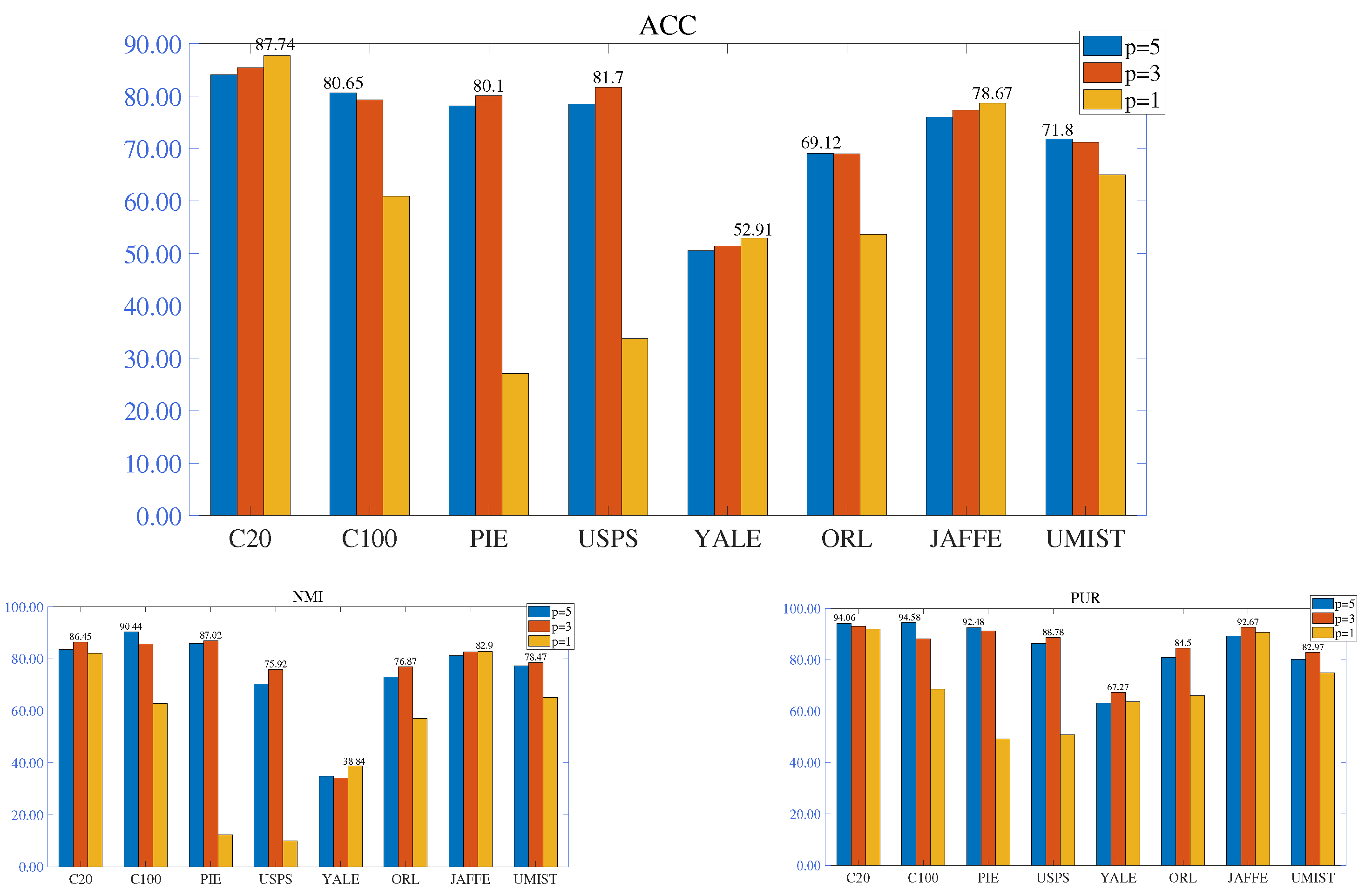
    Parameter p in figure construction is discussed. For the graph in MPCNTD, the nearest neighbours of KNN are set to { 1 , 3 , 5 } . The average classification ACC, NMI and PUR results are reported in Figure 3. Parameter p = 5 , p = 3 and p = 1 are presented in blue, red, and orange columns, respectively. The optimal result can be seen at its columnar top. We found that smaller values are not necessarily better. Due to the strong correlation between points (i.e., data and data) during the graphic construction process, redundant graphic information is generated. Select appropriate p values in practical problems.
  • Hyper-parameter protocol about λ and μ
    There are multiple adjustable regularized parameters λ r , r = U , V , W and μ r , r = U , V , W in our model to balance the fundamental decomposition and consistent regularization terms. To diminish confusion in parameter selection, we set λ r = λ ,   r = U , V , W and μ r = μ ,   r = U , V , W and deeply explore the clustering ability set in this way. The grid control method is considered to acquire the relatively optimal parameters. The numerical selection of two parameters λ , μ is [ 0.001 , 0.01 , 0.1 , 1 , 10 , 100 , 1000 ] by using prior-free criteria. We select 7 × 7 situations to achieve the best clustering effect and provide robustness plots. To weigh the three measurement criteria, the numerical effect of ACC is the essential decisive factor, assisted with NMI and PUR. Specific experimental results are presented in Figure 4.

4.4. Experiments for Effectiveness and Analysis

In this subsection, we apply the maximum number of categories as the number of clusters for the eight datasets, and this is identical treatment for all comparative experimental methods.
From Table 2, our algorithm presents better performance on the eight evaluated datasets. After analyzing the content of Table 2, the following phenomena can be summarized:
(1)
Based on eight image datasets, MPCNTD attains the competent clustering performance in most situations, which demonstrates that MPCNTD can reveal additional discriminative information for tensor data. For example, the average clustering ACC of MPCNTD on the datasets COIL20, COIL100, PIE, USPS, YALE, ORL, JAFFE, and UMIST is higher than the second best method by 3.11%, 2.99%, 1.01%, 5.48%, 6.18%, 3.71%, 2.40% and 2.02%, respectively.
(2)
The matrix dimension reduction approach NMF, GNMF, GDNMF outperform the k-means method with regard to existing outcome. This is because matrix dimension reduction retain more structures of the original data while discovering more accurate data representations. Moreover, the numerical result of NTD-based model is better than that of the NMF-based methods, which illustrates that tensor-based method have advantages over matrix-based methods in data representation and reduction in dimension.
(3)
We found that the NTD method has weak performance in clustering problems because our iteration steps are uniformly set to 100 and we choose a unified initial state. When the iteration process is relaxed and appropriate initial values are selected, this method is still feasible. The result of ONMF losing to NMF is the same. This situation indirectly illustrates that considering consistent regularization not only accelerates the iteration process, but also makes data representation more accurate.
(4)
MPCNTD obtains contestable clustering performance in all experiments. This situation is due to the truth that MPCNTD captures multiple pieces of information from various directions, and this consistent regularization contains graph info and a softly orthogonal structure. Graph learning can maintain the consistency of geometric information of matrices in different spaces, and the balance between multi-graph regularization maximizes the exploration of geometric information of tensor data. The normalization and orthogonality rules in approximate orthogonality work together to maintain data independence as much as possible, resulting in better clustering performance.

4.5. Convergence Study and Running Times

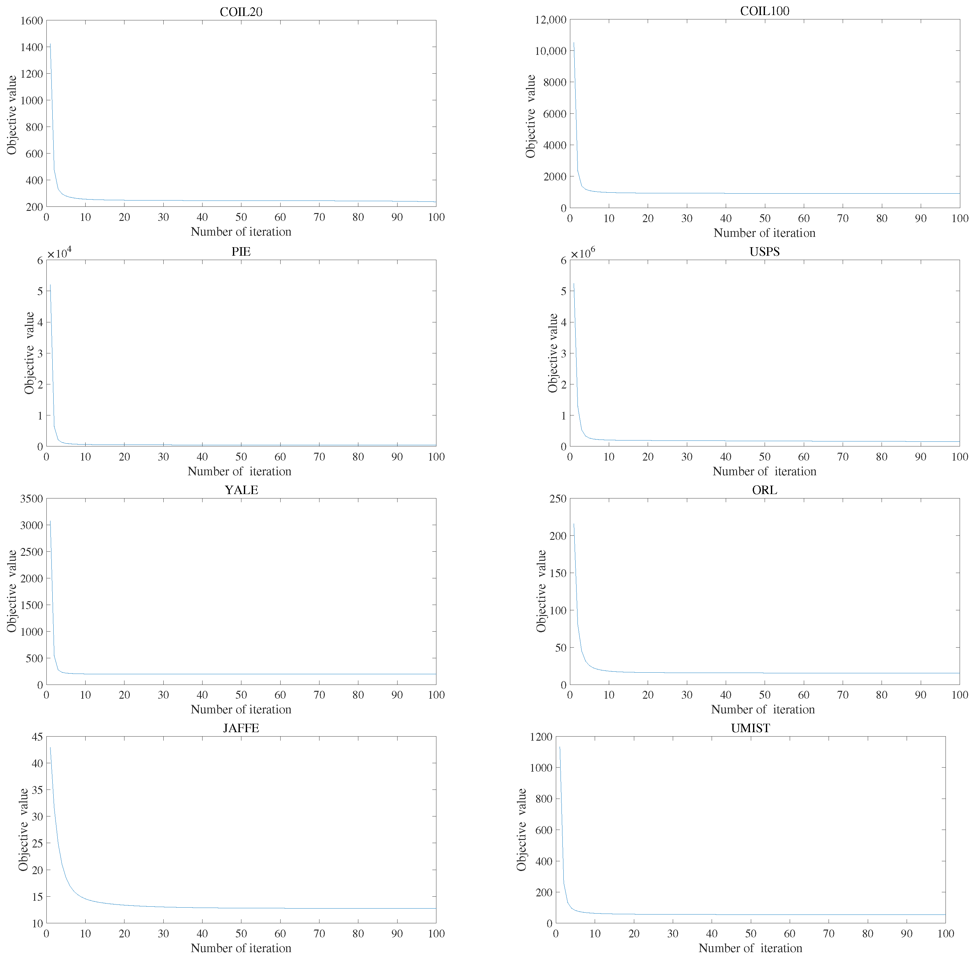
In this part, we pursue the convergence performance of MPCNTD experimentally on all eight evaluated datasets. From Figure 5, we can directly discover that the objective function values are monotonically decreasing and generally reach stability within 50 iterations, which proves the effectiveness of our model and the feasibility of the MU-based iteration method. In addition, we tested the computation time of each method using the maximum number of clusters, and the specific details are described in Table 3. It is not difficult to identify that our method has a longer running time due to the addition of consistent regularization from the comparison of time. But given the superior results, the time consumption can also be tolerated.

5. Conclusions and Expectation

In this article, we propose an NTD-based framework that includes the concepts of graph Laplace and approximate orthogonality, taking into account pairwise constraint in multiple directions. This framework not only utilizes partial representations in tensor models, but also utilizes the structural information of consistent regularization following the decomposition direction. Our proposed model ensures that the minimum point of the objective function converges to the specified local region. Multitudinous experiments were operated on eight real image datasets in unsupervised clustering tasks to make verification and validation of the MPCNTD framework. In the future, we would like to keep on our exploration in the following two aspects. Firstly, it is worth studying whether there are more reasonable constraints to obtain a better solution. More constraint information, such as label information and smoothness, can be considered. Secondly, it is crucial for developing more efficient parallel algorithms about factor matrices. Due to the similarity in the iterative process of factor matrices based on the tensor framework.

Author Contributions

X.G.: Writing—original draft, Validation, Methodology, Conceptualization; L.L.: Writing—review and editing, Supervision, Methodology, Conceptualization. All authors have read and agreed to the published version of the manuscript.

Funding

The work of this paper was supported by the National Natural Science Foundation of China under Grant 12161020 and the National Natural Science Foundation of China under Grant 12061025.

Data Availability Statement

The data presented in this study are available on request from the corresponding author.

Conflicts of Interest

The authors declare no conflicts of interest.

References

  1. Wold, S.; Esbensen, K.; Geladi, P. Principal component analysis. Chemom. Intell. Lab. Syst. 1987, 2, 37–52. [Google Scholar] [CrossRef]
  2. Zhou, G.; Cichocki, A.; Zhang, Y.; Mandic, D.P. Group component analysis for multiblock data: Common and individual feature extraction. IEEE Trans. Neural Netw. Learn. Syst. 2015, 27, 2426–2439. [Google Scholar] [CrossRef] [PubMed]
  3. Lee, D.D.; Seung, H.S. Learning the parts of objects by non-negative matrix factorization. Nature 1999, 401, 788–791. [Google Scholar] [CrossRef] [PubMed]
  4. Lee, D.; Seung, H.S. Algorithms for non-negative matrix factorization. In Proceedings of the 14th International Conference on Neural Information Processing Systems, Denver, CO, USA, 1 January 2000; Volume 13. [Google Scholar]
  5. Kuang, D.; Ding, C.; Park, H. Symmetric nonnegative matrix factorization for graph clustering. In Proceedings of the 2012 SIAM International Conference on Data Mining, SIAM, Anaheim, CA, USA, 26–28 April 2012; pp. 106–117. [Google Scholar]
  6. De Handschutter, P.; Gillis, N. A consistent and flexible framework for deep matrix factorizations. Pattern Recognit. 2023, 134, 109102. [Google Scholar] [CrossRef]
  7. Kolda, T.G.; Bader, B.W. Tensor decompositions and applications. SIAM Rev. 2009, 51, 455–500. [Google Scholar] [CrossRef]
  8. Kim, Y.D.; Choi, S. Nonnegative tucker decomposition. In Proceedings of the 2007 IEEE Conference on Computer Vision and Pattern Recognition, Minneapolis, MN, USA, 17–22 June 2007; pp. 1–8. [Google Scholar]
  9. Wang, Z.; Dellaportas, P.; Kosmidis, I. Bayesian tensor factorisations for time series of counts. Mach. Learn. 2023, 113, 3731–3750. [Google Scholar] [CrossRef]
  10. Yu, Y.; Zhou, G.; Zheng, N.; Qiu, Y.; Xie, S.; Zhao, Q. Graph-regularized non-negative tensor-ring decomposition for multiway representation learning. IEEE Trans. Cybern. 2022, 53, 3114–3127. [Google Scholar] [CrossRef] [PubMed]
  11. Chen, B.; Guan, J.; Li, Z. Unsupervised feature selection via graph regularized nonnegative CP decomposition. IEEE Trans. Pattern Anal. Mach. Intell. 2022, 45, 2582–2594. [Google Scholar] [CrossRef] [PubMed]
  12. Cai, D.; He, X.; Han, J.; Huang, T.S. Graph regularized nonnegative matrix factorization for data representation. IEEE Trans. Pattern Anal. Mach. Intell. 2010, 33, 1548–1560. [Google Scholar] [CrossRef] [PubMed]
  13. Shang, F.; Jiao, L.; Wang, F. Graph dual regularization non-negative matrix factorization for co-clustering. Pattern Recognit. 2012, 45, 2237–2250. [Google Scholar] [CrossRef]
  14. Huang, Q.; Yin, X.; Chen, S.; Wang, Y.; Chen, B. Robust nonnegative matrix factorization with structure regularization. Neurocomputing 2020, 412, 72–90. [Google Scholar] [CrossRef]
  15. Ding, C.; He, X.; Simon, H.D. On the equivalence of nonnegative matrix factorization and spectral clustering. In Proceedings of the 2005 SIAM International Conference on Data Mining, SIAM, Newport Beach, CA, USA, 21–23 April 2005; pp. 606–610. [Google Scholar]
  16. Ding, C.; Li, T.; Peng, W.; Park, H. Orthogonal nonnegative matrix t-factorizations for clustering. In Proceedings of the 12th ACM SIGKDD International Conference on Knowledge Discovery and Data Mining, Philadelphia, PA, USA, 20–23 August 2006; pp. 126–135. [Google Scholar]
  17. Li, B.; Zhou, G.; Cichocki, A. Two efficient algorithms for approximately orthogonal nonnegative matrix factorization. IEEE Signal Process. Lett. 2014, 22, 843–846. [Google Scholar] [CrossRef]
  18. Qiu, Y.; Zhou, G.; Zhang, Y.; Xie, S. Graph regularized nonnegative tucker decomposition for tensor data representation. In Proceedings of the ICASSP 2019—2019 IEEE International Conference on Acoustics, Speech and Signal Processing (ICASSP), Brighton, UK, 12–17 May 2019; pp. 8613–8617. [Google Scholar]
  19. Qiu, Y.; Zhou, G.; Wang, Y.; Zhang, Y.; Xie, S. A generalized graph regularized non-negative tucker decomposition framework for tensor data representation. IEEE Trans. Cybern. 2020, 52, 594–607. [Google Scholar] [CrossRef] [PubMed]
  20. Liu, Q.; Lu, L.; Chen, Z. Nonnegative Tucker Decomposition with Graph Regularization and Smooth Constraint for Clustering. Pattern Recognit. 2023, 148, 110207. [Google Scholar] [CrossRef]
  21. Chen, D.; Zhou, G.; Qiu, Y.; Yu, Y. Adaptive graph regularized non-negative Tucker decomposition for multiway dimensionality reduction. Multimed. Tools Appl. 2024, 83, 9647–9668. [Google Scholar] [CrossRef]
  22. Li, X.; Ng, M.K.; Cong, G.; Ye, Y.; Wu, Q. MR-NTD: Manifold regularization nonnegative tucker decomposition for tensor data dimension reduction and representation. IEEE Trans. Neural Netw. Learn. Syst. 2016, 28, 1787–1800. [Google Scholar] [CrossRef] [PubMed]
  23. Pan, J.; Ng, M.K.; Liu, Y.; Zhang, X.; Yan, H. Orthogonal nonnegative tucker decomposition. SIAM J. Sci. Comput. 2021, 43, B55–B81. [Google Scholar] [CrossRef]
  24. Qiu, Y.; Sun, W.; Zhang, Y.; Gu, X.; Zhou, G. Approximately orthogonal nonnegative Tucker decomposition for flexible multiway clustering. Sci. China Technol. Sci. 2021, 64, 1872–1880. [Google Scholar] [CrossRef]
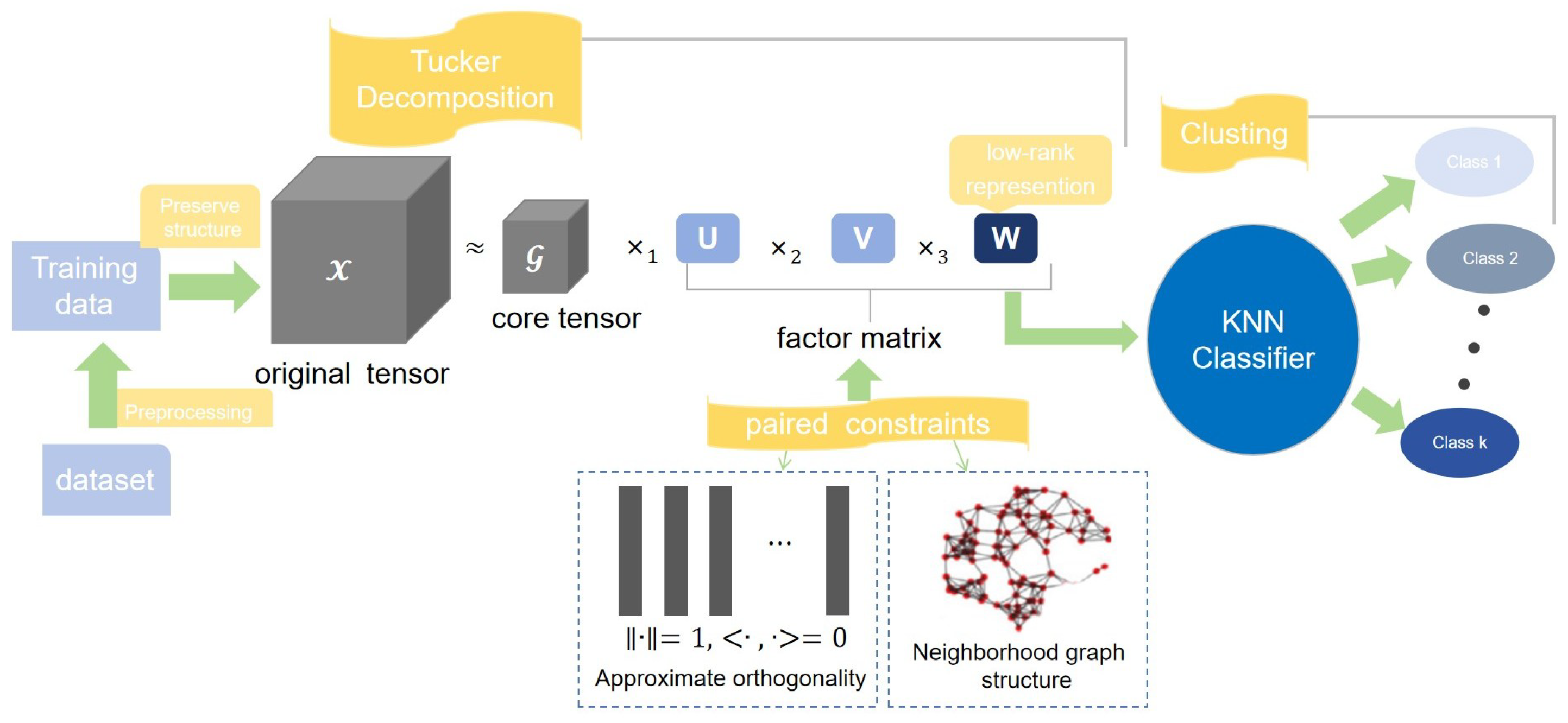
Figure 1. Illustration of the proposed framework.
Symmetry 17 01969 g001
Figure 2. Clustering effect of different sampling ratio.
Symmetry 17 01969 g002
Figure 3. The impact of different graphs on the MPCNTD algorithm.
Symmetry 17 01969 g003
Figure 4. Performance of our method with different parameter settings.
Symmetry 17 01969 g004
Figure 5. Convergence curves of MPCNTD on eight datasets.
Symmetry 17 01969 g005
Table 1. Benchmark dataset.
DatasetsSamplesDimensionsClassesTypeTensor Size
1COIL201440102420Object 32 × 32 × 1440
2COIL10072001024100Object 32 × 32 × 7200
3PIE2856102468Face 32 × 32 × 2856
4USPS929825610Handwritten 16 × 16 × 9298
5YALE165102415Face 32 × 32 × 165
6ORL400102440Face 32 × 32 × 400
7JAFFE213409610Face 64 × 64 × 213
8UMIST575102420Face 32 × 32 × 575
Table 2. Clustering performance based on eight datasets.
K-MeansNMFONMFGNMFGDNMFNTDGNTDMPCNTD
ACC (%)
COIL2053.47 ± 4.0555.37 ± 3.9049.18 ± 1.9169.11 ± 6.8270.05 ± 4.7544.24 ± 2.1969.17 ± 6.6073.16 ± 4.76
COIL10043.91 ± 2.0845.19 ± 1.6037.12 ± 0.9355.69 ± 2.6655.75 ± 2.8121.71 ± 0.3155.98 ± 1.8858.97 ± 1.85
PIE23.84 ± 1.1841.11 ± 2.6821.69 ± 0.4868.17 ± 3.5868.43 ± 4.0953.73 ± 1.4270.31 ± 2.3571.32 ± 2.84
USPS64.46 ± 3.3838.55 ± 1.8036.26 ± 3.5368.77 ± 10.7469.22 ± 10.3527.88 ± 1.4072.34 ± 7.2177.82 ± 12.98
Yale35.58 ± 2.8937.21 ± 1.6235.88 ± 1.8038.48 ± 2.0838.48 ± 2.0836.55 ± 2.0841.03 ± 2.3247.21 ± 2.53
ORL49.87 ± 2.7148.62 ± 2.737.00 ± 0.8951.08 ± 2.0852.17 ± 1.8619.62 ± 0.8451.05 ± 1.5355.88 ± 2.02
JAFFE48.92 ± 4.3145.68 ± 2.8337.79 ± 2.7450.23 ± 4.6458.08 ± 4.6522.58 ± 1.2059.15 ± 3.6061.55 ± 4.37
UMIST40.28 ± 2.1838.12 ± 3.0034.37 ± 1.4860.00 ± 5.5460.45 ± 4.8227.57 ± 1.1760.14 ± 4.9362.47 ± 4.35
NMI (%)
COIL2069.61 ± 1.5669.65 ± 2.3361.87 ± 2.0184.82 ± 3.5084.92 ± 2.2255.13 ± 0.9185.58 ± 2.8186.95 ± 1.68
COIL10072.33 ± 0.8172.41 ± 0.3462.48 ± 0.5179.09 ± 1.4779.31 ± 1.3347.04 ± 0.1180.30 ± 0.7380.31 ± 0.65
PIE53.57 ± 0.6970.30 ± 1.4946.13 ± 0.3985.91 ± 1.3385.88 ± 1.3479.45 ± 0.5285.39 ± 1.1086.60 ± 0.87
USPS60.35 ± 1.4827.09 ± 1.7223.64 ± 3.8678.69 ± 4.3378.61 ± 4.3516.31 ± 0.6978.82 ± 3.0780.83 ± 4.93
Yale40.67 ± 3.9542.06 ± 2.2439.64 ± 1.3044.15 ± 1.7944.13 ± 1.7243.82 ± 2.0747.26 ± 1.6153.51 ± 1.50
ORL69.37 ± 1.4069.11 ± 2.0458.36 ± 0.7870.26 ± 0.9270.17 ± 1.1141.66 ± 0.9270.25 ± 0.6872.98 ± 0.83
JAFFE58.52 ± 2.2856.47 ± 2.4648.44 ± 1.3876.53 ± 2.5376.70 ± 2.2938.94 ± 0.9376.62 ± 2.0277.22 ± 1.81
UMIST52.41 ± 3.7645.40 ± 2.0935.60 ± 2.0257.18 ± 3.4762.30 ± 2.3713.25 ± 1.4161.08 ± 1.9364.79 ± 2.39
PUR (%)
COIL2066.42 ± 2.1465.56 ± 2.4060.18 ± 2.3685.09 ± 3.7085.66 ± 2.8350.85 ± 1.0688.24 ± 2.6987.10 ± 1.61
COIL10057.87 ± 1.1456.84 ± 1.1245.74 ± 0.5072.70 ± 1.2972.48 ± 1.6525.12 ± 0.3870.72 ± 1.3570.02 ± 1.38
PIE29.61 ± 0.8949.52 ± 1.3929.56 ± 0.6984.70 ± 1.2984.85 ± 1.2562.70 ± 1.1983.18 ± 1.3684.68 ± 1.26
USPS70.79 ± 1.7153.18 ± 2.3956.12 ± 5.2484.94 ± 4.1685.30 ± 3.8831.23 ± 1.1184.84 ± 2.6888.52 ± 4.17
Yale48.42 ± 3.6644.61 ± 2.4444.67 ± 1.8345.94 ± 0.9446.00 ± 0.9242.79 ± 2.2548.48 ± 2.4153.33 ± 1.59
ORL59.25 ± 2.6956.63 ± 2.8044.65 ± 1.1258.30 ± 0.7959.25 ± 0.6224.38 ± 1.6058.20 ± 0.9162.60 ± 0.66
JAFFE60.00 ± 4.4352.35 ± 4.0441.31 ± 2.2564.55 ± 3.1968.03 ± 1.8727.42 ± 2.7268.69 ± 1.9870.56 ± 2.53
UMIST45.51 ± 2.2943.29 ± 2.6940.12 ± 1.9869.13 ± 3.2069.23 ± 3.0732.49 ± 1.3769.86 ± 3.1972.35 ± 2.01
Table 3. Running time (seconds).
DatasetsK-MeansNMFONMFGNMFGDNMFNTDGNTDMPCNTD
COIL200.95754.870717.86157.79926.70938.50097.610811.6861
COIL10012.722455.5005389.949259.375960.6811106.429344.929487.1066
PIE4.352318.264977.101419.778119.772384.879134.172436.5172
USPS3.42532.5031179.494410.493111.80639.372834.779044.8650
YALE0.06281.66800.50671.20880.66321.57041.32351.4317
ORL0.26751.54993.21052.07152.38442.13363.40872.3716
JAFFE0.28692.56724.23243.07842.63123.66693.36493.8293
UMIST0.33521.54625.44091.98112.68823.34933.53043.6853
Disclaimer/Publisher’s Note: The statements, opinions and data contained in all publications are solely those of the individual author(s) and contributor(s) and not of MDPI and/or the editor(s). MDPI and/or the editor(s) disclaim responsibility for any injury to people or property resulting from any ideas, methods, instructions or products referred to in the content.