Research on the Influence of Span on Wind Deflection Angle of Insulator Strings in Stochastic Wind Fields

Abstract

This paper presents an independently developed finite element analysis software built on the QT and VTK platforms. Its core innovation is the integration of the analytical solution from catenary theory with nonlinear finite element methods. The software accurately predicts the initial configuration and tension distribution of conductors based on catenary theory, utilizing these results as high-precision initial values for static equilibrium iterations. This approach overcomes the convergence difficulties commonly encountered in traditional commercial software when analyzing such flexible cable structures. Using this software, we systematically investigated the nonlinear effects of asymmetric span arrangements on the mean value and standard deviation of wind deflection angles, and subsequently established a practical wind deflection calculation model that accounts for span asymmetry. The study reveals that higher wind speeds lead to larger wind deflection angles, with static wind deflection angles approximating the mean values under pulsating wind conditions. When one span length is fixed, the wind deflection angle first increases and then decreases as the adjacent span length increases. Symmetrical span arrangements were found to amplify the fluctuation range of the wind deflection angles. The research further developed polynomial regression models to systematically analyze the influence of wind speed and span length on dynamic amplification factors and elucidate their interactions and nonlinear relationships. Finally, based on symbolic regression and least squares methods, three expressions for the dynamic amplification factor in terms of span length and wind speed were derived. These formulas all demonstrate certain engineering applicability for predicting the dynamic amplification factor.

1. Introduction

The operational safety of overhead transmission lines during extreme weather events, particularly under strong wind conditions, has become an increasingly critical concern in recent years. Wind-induced flashover accidents, where strong winds cause significant wind deflection of insulator strings and conductors, reducing the air gap between the conductor and the tower below the critical discharge distance, pose a substantial threat to grid stability [1,2]. The global increase in extreme wind events and the imperative to construct transmission lines in complex, high-altitude regions (e.g., hydropower projects in China’s Yarlung Zangbo River basin) underscore the urgent need for in-depth research into transmission line wind deflection phenomena [3,4].

Early research on wind-induced deflection of transmission lines primarily focused on experimental analysis [5,6,7] and static calculation methods [8], which established a fundamental understanding but often neglected the complex influence of wind on conductors. With advancements in computational technology, the finite element method has been widely applied to dynamic analysis of transmission line wind deflection, enabling the capture of more intricate nonlinear transient processes. McClure and Lapointe (2003) [9] introduced a finite element-based modeling framework for analyzing the dynamic response of overhead transmission lines. Bo Yan et al. (2009) [10] utilized ABAQUS software for numerical simulation of the dynamic swing of suspension insulator strings in a random wind field, revealing that dynamic wind deflection angles often exceed conventional design specifications. Diana et al. (1998) [11] developed a nonlinear finite element model to systematically analyze wind-induced vibrations in large-span transmission line crossings and emphasized the importance of optimizing damping devices. To comprehensively understand wind-induced flashover, researchers have investigated various influencing factors. For instance, An et al. (2019) [12] explored flashover mechanisms under combined wind and rain conditions. Liu et al. (2024) [13] analyzed the impact of parameters such as span and height difference on wind deflection based on meteorological predictions. Li et al. (2021) [14] elucidated the amplifying effect of icing coupled with wind speed on wind deflection angles. In terms of wind deflection mitigation techniques, Song et al. (2024) [15] introduced a novel spring-pendulum dynamic vibration absorber (SPDVA) to suppress the wind-induced response of large-span transmission tower-line systems, demonstrating superior effectiveness. Furthermore, research has extended to complex vibration behaviors of transmission lines. Chen et al. (2025) [16] analyzed the stability of parametric vibrations in overhead conductors under time-varying tension and proposed engineering recommendations for span adjustments. Regarding optimization of wind deflection calculation models, Zhao et al. (2022) [17] proposed a simplified calculation model based on the rigid body criterion and the load-response-correlation (LRC) method, innovatively decoupling the wind deflection process into “rigid body displacement under mean wind + small-amplitude vibration under pulsating wind,” significantly enhancing prediction accuracy. The studies by Tripathi A.N. (2023) [18] validated the effectiveness of increasing insulator string weight to suppress wind deflection, while Bao et al. (2022) [19] validated a non-linear buckling analysis modeling method for Y-type insulators. Faced with the escalating challenges posed by extreme weather events to power systems, enhancing grid resilience and risk assessment has become a prominent research area. Fatima and Shareef (2025) [20] developed a dynamic Bayesian network (DBN) model for assessing fault probabilities in overhead power lines affected by hurricanes. Goulioti et al. (2025) [21] constructed a smart-grid resilience enhancement framework based on high-impact high-frequency (HIHF) event models, integrating historical meteorological data, machine learning, and multi-criteria decision-making methods to provide data-driven support for grid response to extreme events. Reda Snaiki (2024) [22] proposed a data-driven multi-scale risk assessment framework to address coupled risks from multi-hazards such as ice storms, offering new perspectives for preventing wind-induced flashover accidents. Zhao S et al. (2025) [23] introduced extreme-value combination rules for tower-line systems under non-Gaussian wind-induced vibration response. Hou et al. (2022) [24] significantly improved the accuracy of wind-induced flashover risk prediction for transmission lines in typhoon-prone areas by incorporating risk mapping logic from the GBR model. Qian et al. (2021) [25] found that the axial pressure and turbulent energy variations at the composite insulator core rod connections were most significant, making these areas prone to stress concentration. Compared to V-type insulator strings, the wind pressure and turbulence fluctuations of suspension insulator strings in wind fields demonstrated greater stability. Qian et al. (2022) [26] emphasized that nonlinear effects in hundred-meter-scale blades substantially influence aeroelastic characteristics, including dynamic response and edgewise vibration modes. Consequently, nonlinear aeroelastic effects must be thoroughly considered during blade design to ensure operational safety of wind turbines. Tian et al. (2025) [27] established the dynamic equations for coupled horizontal and vertical vibrations of structures under along-wind fluctuating excitations. Utilizing finite element analysis techniques, they obtained real modal dynamic parameters of long-span suspended structures and reconstructed the dynamic equations of the vibration control system based on real modal theory. The validity of the proposed closed-form solutions was verified through numerical examples, based on which the characteristics of inerter system parameters for suppressing bidirectional wind-induced vibrations of suspended structures were systematically investigated. While substantial research has been conducted on the wind-induced response of transmission tower-line systems, the necessity of this study stems from a critical, yet long-overlooked aspect: to elucidate the decisive influence of span length—a key design parameter—on the dynamic behavior of suspension insulator strings, which are critical load-bearing and insulating components, under pulsating wind loads.

In summary, despite substantial research achievements in the field of transmission line wind deflection, detailed investigations into the impact of line structural parameters on suspension insulator string wind deflection under dynamic pulsating wind effects remain to be thoroughly explored. Building upon the aforementioned research, this paper develops a finite element software for transmission line conductor simulation, implemented in C++ on the VTK and QT platforms. By establishing models of insulator strings and transmission conductors with varying spans based on actual high-voltage transmission lines, this study focuses on investigating the influence mechanisms of line structural parameters, such as span, on the wind deflection of suspension insulator strings under dynamic pulsating wind conditions. The aim is to provide a more precise theoretical basis and technical support for the design, operation, and safety assessment of transmission lines.

2. Finite Element Modeling and Validation of Transmission Line Simulation

2.1. Geometric Stiffness Matrix of Space Truss Elements Considering Geometric Nonlinearity

As a typical flexible structure, the conductor exhibits mechanical behavior characterized by small strain and large displacement, leading to significant geometric nonlinearity. For such geometric nonlinearity problems, Lou et al. (2022) [28] adopted three-node cable elements to model transmission lines, while Huang et al. (2023) [29] employed beam elements for conductor simulation. To accurately model this, the conductor in this study is represented by co-rotational truss elements. This approach is also applied to the simulation of insulator strings [30].

Figure 1 illustrates a space truss element that has undergone large rotation and small deformation, transitioning from its initial to its current configuration.

In the global coordinate system xyz, let (⁰x_i, ⁰y_i, ⁰z_i) and (^tx_i, ^ty_i, ^tz_i) represent the coordinates of the i-th node of the truss element at the initial moment and an arbitrary time t, respectively. Subtracting these two sets of coordinates yields the nodal displacement of the element in the global coordinate system, which can be expressed as:

$$U^e={[u_i\hspace{1em}{v}_i\hspace{1em}{w}_i\hspace{1em}{u}_j\hspace{1em}{v}_j\hspace{1em}{w}_j]}^{\mathrm{T}}$$

(1)

In the above formula, U^e represents the node displacement vector of the truss element. In the formula, u, v, and w are the displacement components along the three degrees of freedom within the overall coordinate system. The original length of the truss element, as defined in the initial configuration, is:

$$l_0=\sqrt{{({}^{0}x_j-{}^{0}x_i)}^2+{({}^{0}y_j-{}^{0}y_i)}^2+{({}^{0}z_j-{}^{0}z_i)}^2}$$

(2)

The length after deformation is:

$$l_t=\sqrt{{({}^{0}x_j-{}^{0}x_i+u_j-u_i)}^2+{({}^{0}y_j-{}^{0}y_i+v_j-v_i)}^2+{({}^{0}z_j-{}^{0}z_i+w_j-w_i)}^2}$$

(3)

The elongation of this element is:

$$\Delta l=l_t-l_0$$

(4)

Under the assumptions of small deformation and linear elasticity, the axial force in a truss element at nodes i and j is:

$${\overline{N}}_i=-{\displaystyle \frac{EA}{l_0}}\Delta l , {\overline{N}}_j={\displaystyle \frac{EA}{l_0}}\Delta l$$

(5)

In the formulas, E and A represent the elastic modulus and cross-sectional area of the truss element, respectively.

Let α, β and γ be the angles between the deformed truss element and the x, y and z axes of the global coordinate system, respectively. Then:

$$c_1=\cos \alpha =({}^{0}x_j-{}^{0}x_i+u_j-u_i)/l_t , s_1=\sin \alpha$$

(6a)

$$c_2=\cos \beta =({}^{0}y_j-{}^{0}y_i+v_j-v_i)/l_t , s_2=\sin \beta$$

(6b)

$$c_3=\cos \gamma =({}^{0}z_j-{}^{0}z_i+w_j-w_i)/l_t , s_3=\sin \gamma$$

(6c)

By projecting the axial forces of nodes i and j (represented by ${\overline{N}}_i$ and ${\overline{N}}_j$) onto the three global coordinate system axes and differentiating, we obtain:

$$\delta F_{xi}=\delta {\overline{N}}_i{c}_1-{\overline{N}}_i{s}_1\delta \alpha ; \delta F_{yi}=\delta {\overline{N}}_i{c}_2-{\overline{N}}_i{s}_2\delta \beta ; \delta F_{z_i}=\delta {\overline{N}}_i{c}_3-{\overline{N}}_i{s}_3\delta \gamma$$

(7)

By differentiating Equations (6) and (7), we obtain:

$$\delta \Delta l=\left[\begin{array}{cccccc}-c_1& -c_2& -c_3& c_1& c_2& c_3\end{array}\right]\delta U^e$$

(8a)

$$\delta \alpha ={\displaystyle \frac{1}{l_t{s}_1}}\left[\begin{array}{cccccc}{s}_1^2& -c_1{c}_2& -c_1{c}_3& -s_1^2& c_1{c}_2& c_1{c}_3\end{array}\right]\delta U^e$$

(8b)

$$\delta \beta ={\displaystyle \frac{1}{l_t{s}_2}}\left[\begin{array}{cccccc}-c_1{c}_2& s_2^2& -c_2{c}_3& c_1{c}_2& -s_2^2& c_2{c}_3\end{array}\right]\delta U^e$$

(8c)

$$\delta \gamma ={\displaystyle \frac{1}{l_t{s}_3}}\left[\begin{array}{cccccc}-c_1{c}_3& -c_3{c}_2& s_3^2& c_1{c}_3& c_3{c}_2& -s_3^2\end{array}\right]\delta U^e$$

(8d)

In these formulas, $\delta U^e$ is defined as:

$$\delta U^e={\left[\begin{array}{cccccc}\delta u_i& \delta v_i& \delta w_i& \delta u_j& \delta v_j& \delta w_j\end{array}\right]}^{\mathrm{T}}$$

Substituting Equation (8) into Equation (7) yields the relationship between the incremental forces at the ends of truss elements, $\delta F$, and the incremental displacements in a spatial truss under large rotational deformation, $\delta U^e$. This relationship is represented by the tangent stiffness matrix K_T:

$$\delta F=K_{\mathrm{T}}\delta U=(K_{\mathrm{L}}+K_{\mathrm{N}})\delta U^e$$

(9)

The matrix K_T can be found in the literature [31].

2.2. Dynamic Solution Based on Newmark-β Method

This paper uses the Newmark-β implicit algorithm to perform time integration of the full wind-induced deflection process of transmission lines [32]. This approach avoids the use of complex geometrically nonlinear constitutive relations. By dynamically adjusting the iterative convergence tolerance based on the structural dynamic response, computational effort is saved while ensuring accuracy. The procedure for solving the structural dynamic response at time t + Δt is outlined below:

(1)

Initialize the displacement, velocity, and acceleration at t + Δt as ${}^{t+\Delta t}\mathbf{u}_0$, ${}^{t+\Delta t}\dot{\mathbf{u}}_0$ and ${}^{t+\Delta t}\ddot{\mathbf{u}}_0$, respectively, where the subscript ‘0’ denotes the initial iteration. The initial displacement at time t + Δt is initialized using the converged displacement at time t, while the velocity and acceleration are estimated as:

$$\begin{array}{c}{}^{t+\Delta t}\ddot{\mathbf{u}}_0=-{\displaystyle \frac{1}{\beta \Delta t}}\left({}^t\dot{\mathbf{u}}\right)-\left({\displaystyle \frac{1}{2\beta }}-1\right)\left({}^t\ddot{\mathbf{u}}\right)\end{array}$$

(10a)

$${}^{t+\Delta t}\dot{\mathbf{u}}_0=\left(1-{\displaystyle \frac{\gamma }{\beta }}\right)\left({}^t\dot{\mathbf{u}}\right)+\left(1-{\displaystyle \frac{\gamma }{2\beta }}\right)\Delta t\left({}^t\ddot{\mathbf{u}}\right)$$

(10b)

(2)

Form the stiffness matrix ${}^{t+\Delta t}K_n$, mass matrix ${}^{t+\Delta t}\mathbf{M}_n$, and damping matrix ${}^{t+\Delta t}C_n$ for the nth iteration.

(3)

Assemble the equivalent stiffness matrix:

$${}^{t+\Delta t}\tilde{\mathbf{K}}_n={\displaystyle \frac{1}{\beta \Delta t^2}}{\cdot }^{t+\Delta t}{M}_n+{\displaystyle \frac{\gamma }{\beta \Delta t}}{\cdot }^{t+\Delta t}{C}_n{+}^{t+\Delta t}{K}_n$$

(11)

(4)

Compute the equivalent load vector at t + Δt:

$${}^{t+\Delta t}\tilde{\mathbf{F}}_{n+1}{=}^{t+\Delta t}{F}_{n+1}{-}^{t+\Delta t}{M}_n{\cdot }^{t+\Delta t}{\ddot{u}}_n{-}^{t+\Delta t}{C}_n{\cdot }^{t+\Delta t}{\dot{u}}_n$$

(12)

(5)

Solve for the displacement increment:

$${}^{t+\Delta t}\Delta u_{n+1}={\left({}^{t+\Delta t}\tilde{K}_n\right)}^{-1}{}^{t+\Delta t}\tilde{F}_{n+1}$$

(13)

(6)

Update the displacement:

$${}^{t+\Delta t}\mathbf{u}_{n+1}{=}^{t+\Delta t}{u}_n{+}^{t+\Delta t}\Delta u_{n+1}$$

(14)

(7)

Update the velocity and acceleration to complete the recursion:

$${}^{t+\Delta t}\dot{\mathbf{u}}_{n+1}{=}^{t+\Delta t}{\dot{u}}_n+{\displaystyle \frac{\gamma }{\beta \Delta t}}\left({}^{t+\Delta t}\mathbf{u}_{n+1}{-}^{t+\Delta t}{u}_n\right)$$

(15a)

$${}^{t+\Delta t}\ddot{\mathbf{u}}_{n+1}{=}^{t+\Delta t}{\ddot{u}}_n+{\displaystyle \frac{1}{\beta \Delta t^2}}\left({}^{t+\Delta t}\mathbf{u}_{n+1}{-}^{t+\Delta t}{u}_n\right)$$

(15b)

Regarding the implicit solution method for equations, the termination of iteration is determined by the convergence criterion. In this study, the judgment of convergence is based on the magnitude of the displacement increment, specifically employing the displacement increment error criterion [33,34]:

$${\displaystyle \frac{{\left|{}^{t+\Delta t}\mathbf{u}_{n+1}\right|}_{L_2}}{{\left|{}^{t+\Delta t}\mathbf{u}_{n+1}{-}^{t+\Delta t}{u}_0\right|}_{L_2}}}\le \eta$$

(16)

The L₂ norm is appropriate when controlling the average error across all degrees of freedom is required. In the equation above, ${}^{t+\Delta t}\mathbf{u}_{n+1}$ represents the displacement increment vector at all nodes during the (n + 1)th iteration at time ${}^{t+\Delta t}\mathbf{u}_{n+1}{-}^{t+\Delta t}{u}_0$ denotes the total displacement increment after n + 1 iterations at time t + Δt, and η is a proportional factor controlling the error, referred to as the convergence tolerance.

The selection of the convergence tolerance η must be approached with great caution, as it governs both computational speed and accuracy. If the criterion is too lenient, the solution may become highly inaccurate and unstable; conversely, an excessively strict criterion will significantly increase computational time, leading to unnecessary iterative calculations. In this study, the value of the convergence tolerance η was ultimately determined through comparative analysis of numerical examples.

2.3. Wire Shape Verification

The span of transmission lines is typically substantial, generally ranging from 100 to 1000 m. Taking the LGJ-400/50 conductor as an example, its outer diameter is 27.63 mm, which is considerably smaller than the span dimensions. Additionally, its bending strain energy is significantly lower than its tensile strain energy. Therefore, truss elements are commonly employed in engineering analysis for simulation.

However, using truss elements to model conductors has certain limitations. When multiple elements are used to discretize the structure for static analysis, the transmission line, as a highly flexible kinematic system, tends to cause difficulties in numerical convergence. This issue is also relatively common in mainstream commercial finite element software.

To address the aforementioned convergence issues, this study utilizes catenary theory to directly obtain the precise initial geometry of the conductor under self-weight and establishes the axial forces in each element as the initial internal force state, thereby achieving efficient form-finding for the transmission line model. According to catenary theory, given the horizontal coordinate x of any point, its vertical coordinate y can be expressed as:

$$y={\displaystyle \frac{2H}{mg}}\mathrm{sh}{\displaystyle \frac{mgx}{2H}}\mathrm{sh}{\displaystyle \frac{mg(x-2a)}{2H}}$$

(17)

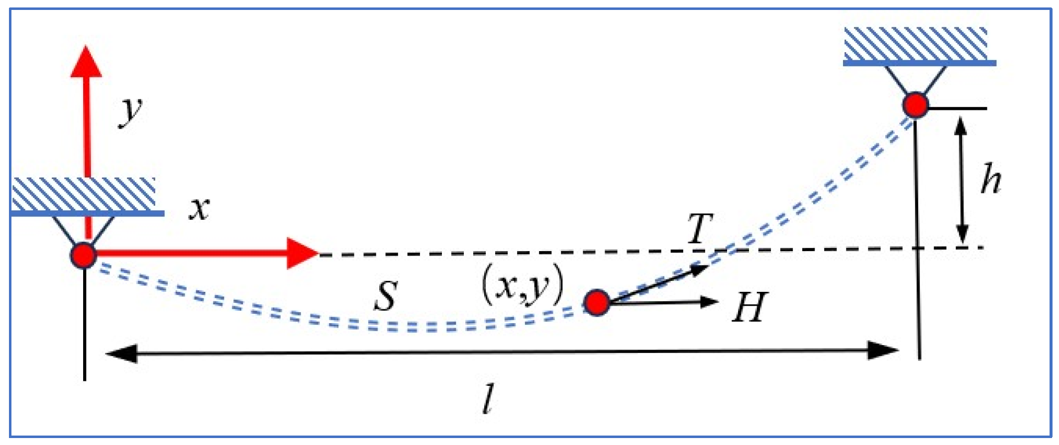
In the formula, mg denotes the weight per unit length of the conductor, T represents the horizontal tension under the conductor’s self-weight, and sh is the hyperbolic sine function. The parameter a in the above equation is:

$$a={\displaystyle \frac{l}{2}}-{\displaystyle \frac{H}{mg}}\mathrm{arsh}{\displaystyle \frac{h}{\frac{2H}{mg}\mathrm{sh}\frac{mgl}{2H}}}$$

(18)

In the above formula, l represents the horizontal span, and h represents the height difference. Based on Equation (1), the coordinates of any point on the transmission line under a given tension or sag can be obtained. According to the calculation formula along the line, the tension T at any point can be expressed as:

$$T=\sqrt{H^2+mgS}$$

(19)

In the above formula, S represents the distance between the left suspension point and any arbitrary point, with the various parameters illustrated in Figure 2.

The software constructs a three-span conductor model based on the catenary formula, using LGJ-400/50 type conductor with a cross-sectional area A = 3.389 × 10⁻⁴ m², elastic modulus E = 6.9 × 10⁹ Pa, Poisson’s ratio ν = 0.3, density ρ = 3346 kg/m³, and a minimum point stress of 64.61 MPa. Each span of the conductor is divided into 100 elements for gravitational analysis. Since the initial configuration strictly satisfies the catenary theory, the static iteration converges in only two steps, significantly improving computational efficiency and numerical stability. the three-span conductor line structure in Figure 3.

Table 1. Results of Multi-Span Conductor Shape Finding.

Span	Length (m)	Height Difference (m)	Theoretical Sag (m)	Computed Sag (m)	Error (%)
1	500	50	15.8434	15.8441	0.00444
2	200	0	2.5276	2.5275	−0.00336
3	700	−100	31.2775	31.2776	0.00025

details the model information and the form-finding results. The results show that the maximum mid-span sag error obtained through form-finding in this case is only 0.0044%, validating the high efficiency and accuracy of the software in transmission line form-finding. The selection of cable elements, which sustain only tensile loads, is dictated by an accurate representation of the conductor’s physical nature. This approach is adopted to ensure the accuracy of dynamic response simulations and to maintain computational efficiency, thereby facilitating parametric studies and convergence analysis.

2.4. Forced Dynamic Response Verification

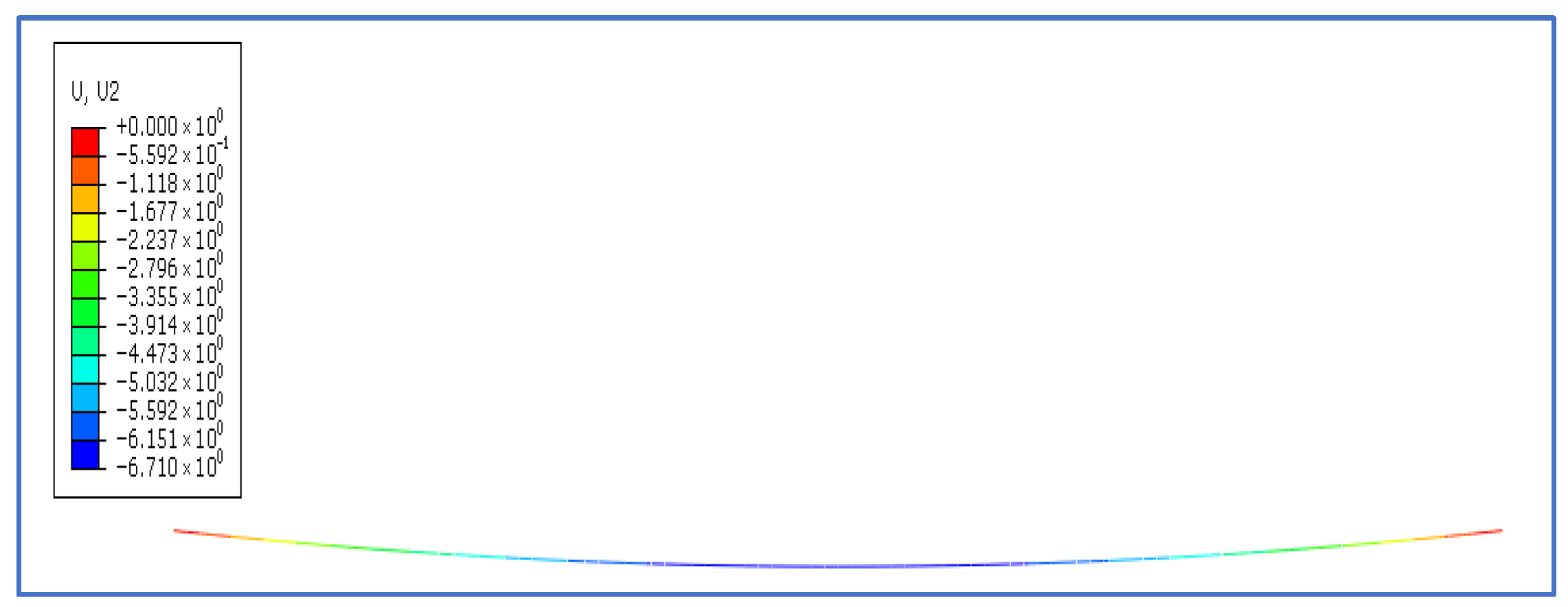
To validate the accuracy of the truss element model, this study employs the following specific example. A conductor wire of type LGJ-400/50 with a span of 400 m is modeled. The conductor is divided into 100 elements, and the model is discretized in ABAQUS 2022 using 100 two-node truss elements. ABAQUS performs a self-weight analysis to obtain the displacement of the conductor in static equilibrium, as shown in Figure 4.

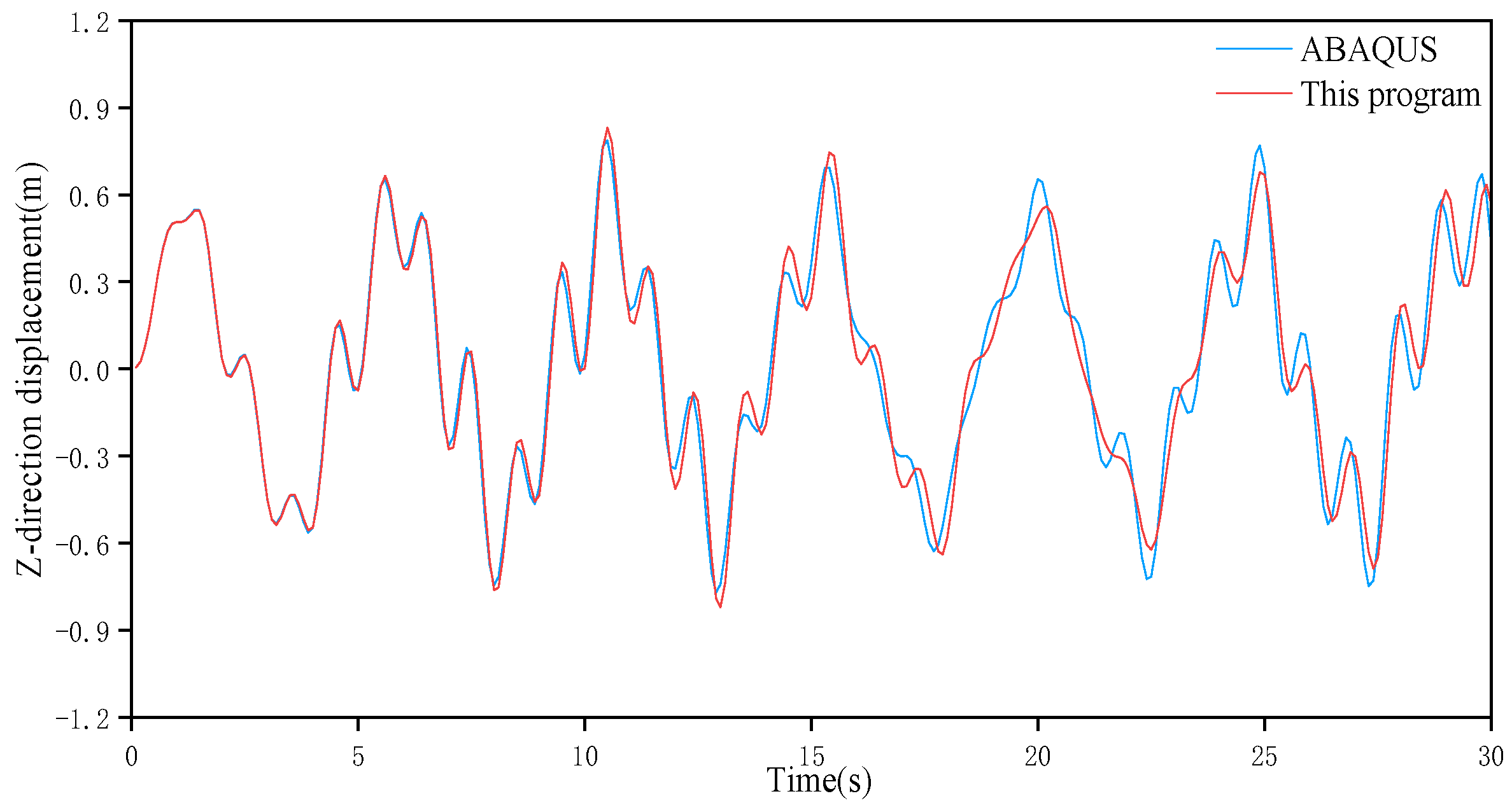
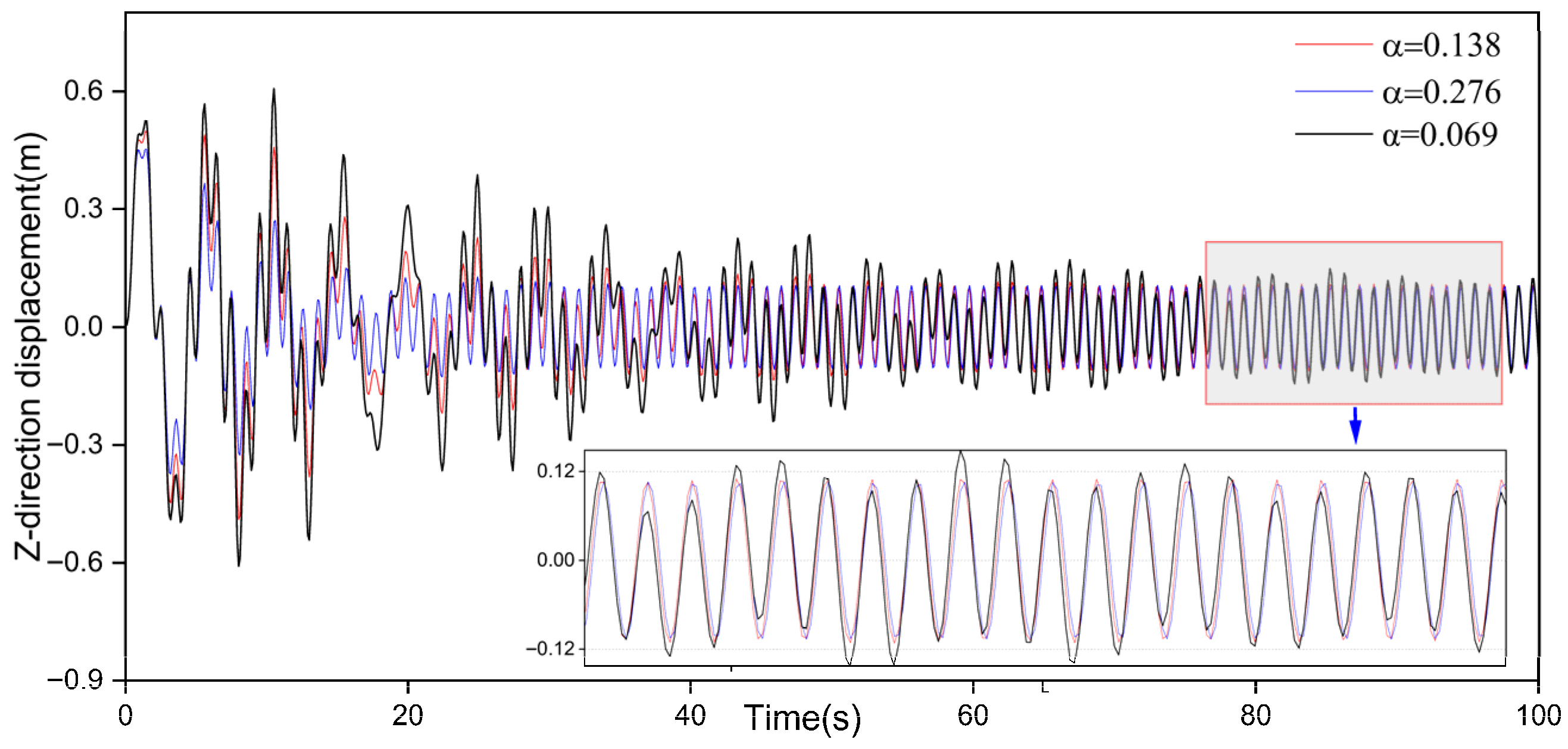
Figure 4 indicates that the maximum sag of the conductor is 6.71 m. The result from the self-weight analysis conducted by the present software yields a maximum sag of 6.712 m, showing only a negligible discrepancy between the two. Subsequently, a body force along the Z-direction is applied to the entire conductor, with the time-dependent variation defined as F(t) = 1000·f(t), were f(t) = sin(6.14·t). The time step for dynamic analysis is set to Δt = 0.1 s, and both damped and undamped conditions are considered. Under damped conditions, Rayleigh damping is adopted: C = αM + βK, with coefficients set to α = 0.138 and β = 0.

Figure 5 and Figure 6 present the time history of the transverse displacement at the midpoint of the conductor, as computed by the present software and ABAQUS, under undamped and damped conditions, respectively. It can be observed that the program developed in this study effectively captures the phenomena of free vibration, coupled vibration, and forced vibration. The frequency and peak values of the displacement responses show close agreement with those from ABAQUS. This demonstrates the software’s capability to handle dynamic response scenarios both with and without damping, confirms its accuracy in addressing complex dynamic problems, and validates its effectiveness in calculating the wind-induced deflection of transmission lines.

To further investigate the influence of damping on system parameters, this study examines the effect of variations in the α coefficient on the vertical displacement of the system, with the results shown in Figure 7. As observed in the figure, with increasing damping, the vibrational displacement of the system within the first 20 s attenuates significantly. When α = 0.276, the vertical vibrational displacement stabilizes around 20 s; whereas in the case of α = 0.069, the vibrational displacement remains relatively large. As the vibration time approaches 100 s, the computational results under the three cases converge, indicating that the damping ratio has a weak influence on the final steady-state response of the system.

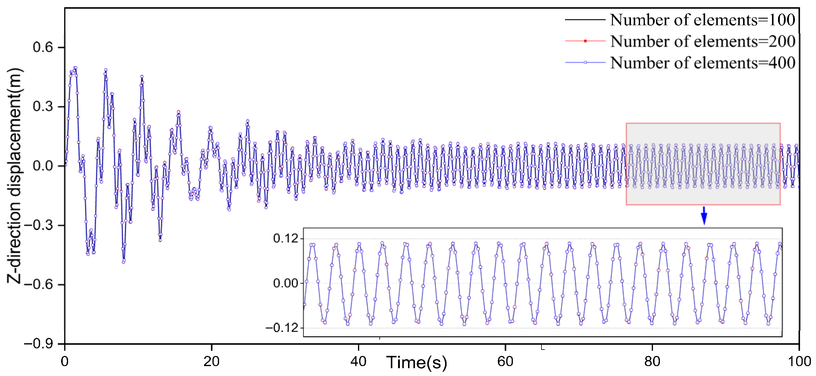
To further investigate the influence of element quantity on computational results, this study analyzes the effects of different element discretizations on numerical outcomes, as shown in the figure below. In the Figure 8, the solid black line represents the computational results obtained with 100 elements, the red scatter points correspond to 200 elements, and the blue square scatter points denote 400 elements. It can be observed that the three curves essentially coincide, indicating that using 100 elements is sufficient to achieve reasonably accurate computational results when simulating flexible conductors. Moreover, it is worth noting that when three distinct mesh generation approaches were employed to solve the vibration problem, the final iteration count remained consistently at 1001 across all cases, unaffected by variations in element quantity.

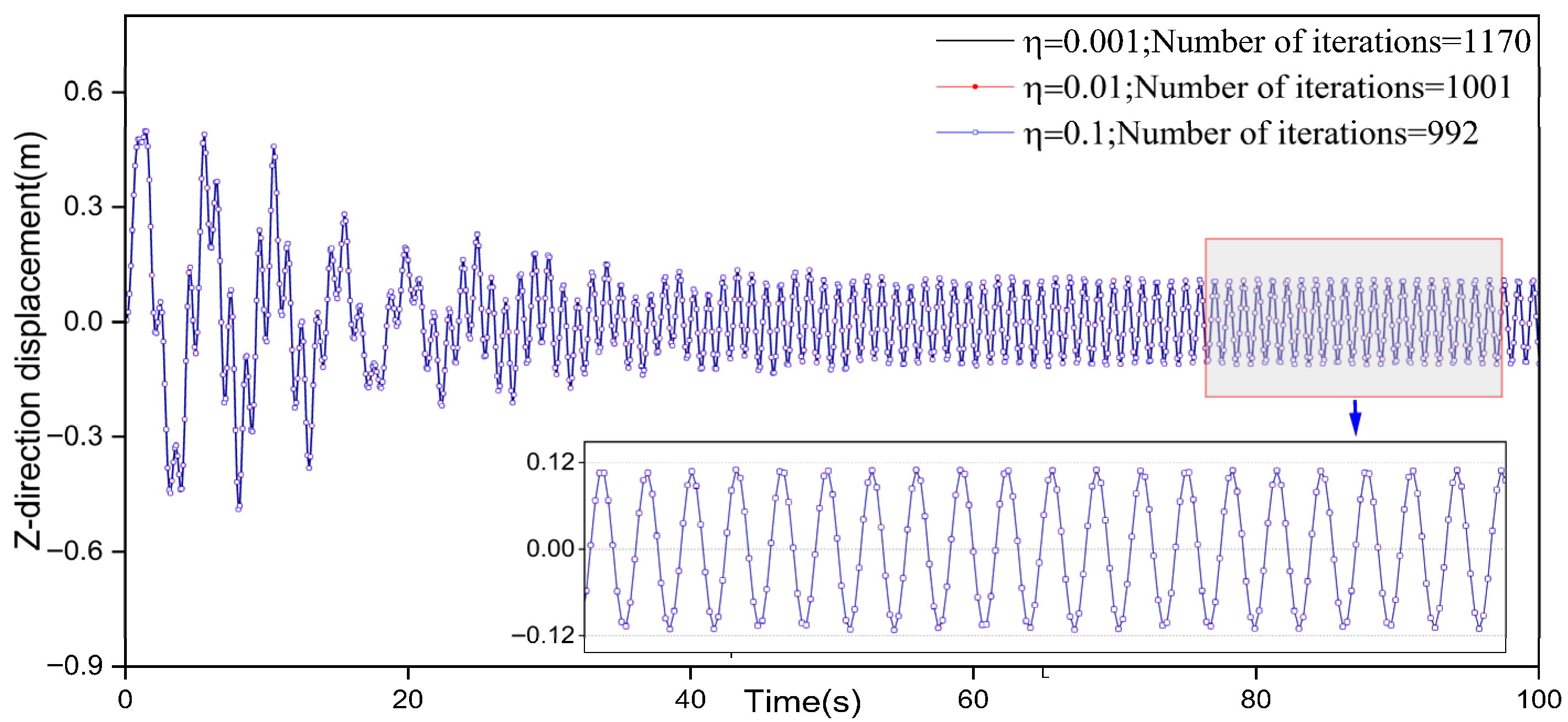
To further evaluate the influence of the iterative convergence tolerance on numerical results, this study conducted a comparative analysis of computational outcomes under three tolerance values: η = 0.1, 0.01, and 0.001. As shown in Figure 9, the displacement time-history curves under different tolerance settings are essentially identical, indicating that the computational results for this particular problem are insensitive to variations in η. Figure 9 further reveals that the corresponding iteration counts for convergence tolerance values of 0.1, 0.01, and 0.001 are 992, 1001, and 1170, respectively. Considering that a looser tolerance (e.g., η = 0.1) may lead to loss of accuracy, while a stricter tolerance (e.g., η = 0.001) would significantly increase computational time, this study ultimately selects η = 0.01 as the iterative convergence tolerance to balance computational efficiency with numerical accuracy.

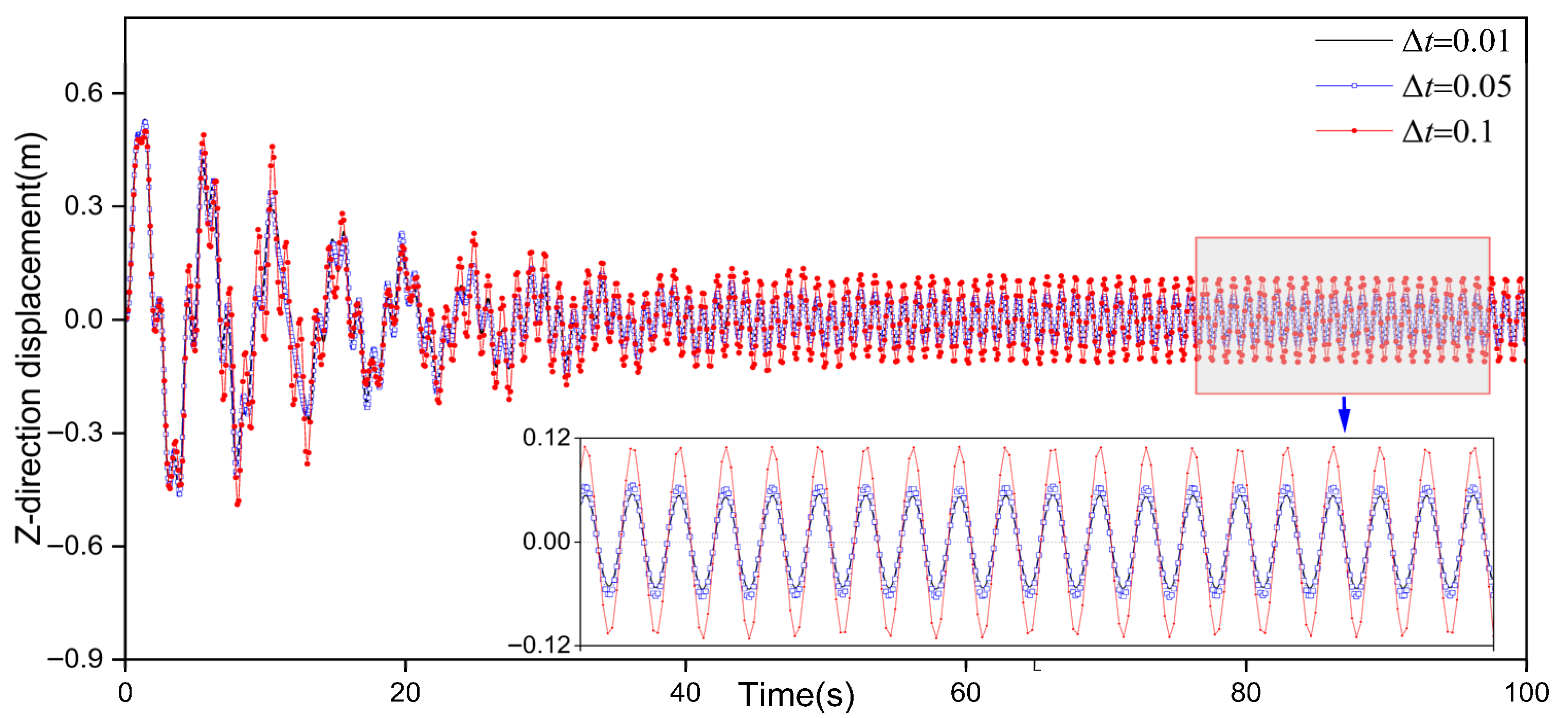
To further evaluate the impact of time increment (Δt) on computational accuracy and efficiency, this study comparatively analyzes dynamic responses under three values: Δt = 0.1 s, 0.05 s, and 0.01 s. As shown in Figure 10, when Δt = 0.1 s, the calculated displacement is significantly larger, indicating that an excessive step size leads to considerable numerical errors. When the step size is reduced to 0.05 s and 0.01 s, the results from both are very close, suggesting that the solution has converged. Since Δt = 0.05 s ensures computational accuracy while providing better efficiency than Δt = 0.01 s, this study ultimately selects 0.05 s as the time step for subsequent wind-induced response analysis.

While the modeling methodology and parameter selection in this study have undergone rigorous validation against commercial software, the following limitation persists: the absence of field-measured response data from actual transmission lines under wind loads precludes more comprehensive experimental verification.

3. The Impact of Span on Wind-Induced Deflection Response

3.1. Simulation of Wind Field

While factors such as typhoons (generating strongly non-stationary wind fields), wake flows behind gentle and moderately sloped hills, flow separation, and vortex shedding (which induce pronounced non-Gaussian characteristics in local wind pressure distributions) can introduce non-Gaussian characteristics to wind [35,36], this study focuses on general conditions in engineering wind-resistant design and adopts the assumption that wind follows a Gaussian stationary random process.

Wind speed spectra commonly used in the simulation of pulsating wind include the Davenport spectrum, Kaimal spectrum, and Harris spectrum, among others. This study adopts the Kaimal spectrum, which is expressed as:

$$\left\{\begin{array}{c}{S}_v(z,f)={\displaystyle \frac{200f_{\ast }{V}_{\ast }^2}{f{(1+50f_{\ast })}^{5/3}}} , V_{\ast }=0.35{\displaystyle \frac{\overline{V}(z)}{\mathrm{In}\frac{z}{z_0}}}\\ x={\displaystyle \frac{1200f}{{\overline{v}}_{10}}} , \overline{V}\left(\mathrm{z}\right)={\overline{V}}_{10}{\left({\displaystyle \frac{z}{10}}\right)}^{\alpha }\end{array}\right.$$

(20)

where $V_{\ast }$ denotes the friction velocity, $f_{\ast }$ is the Mohrisch–Coulomb coordinate, $\overline{V}(z)$ is the average wind speed at z (m/s), ${\overline{V}}_{10}$ is the reference wind speed at 10 m height (m/s), f = ω/2π is the frequency (Hz), z is the height (m), z₀ is the ground roughness length, and α is the ground roughness coefficient.

The harmonic superposition method is employed to simulate the pulsating wind field. Pulsating wind can be modeled as a zero-mean stationary Gaussian process. Consider n such processes $v_j(t)$ (j = 1, 2, …, n). Their spectral density function matrix is given by:

$$\mathit{S}(\omega )=\left[\begin{array}{cccc}{S}_{11}(\omega )& S_{12}(\omega )& \cdots & S_{1n}(\omega )\\ S_{21}(\omega )& S_{22}(\omega )& \cdots & S_{2n}(\omega )\\ \cdots & \cdots & \cdots & \cdots \\ S_{n1}(\omega )& S_{n2}(\omega )& \cdots & S_{nn}(\omega )\end{array}\right]$$

(21)

Here, $S(\omega )$ is a positive definite matrix, and each element in the matrix can be calculated by the following formula:

$$S_{kl}(r,f)=\sqrt{S_{kk}(z_k,f)S_{ll}(z_l,f)}\mathrm{Coh}(r,f)e^{i\theta (f)}, k\ne l$$

(22)

In the equation, $S_{kk}(z_k,f)$ and $S_{ll}(z_l,f)$ represent the auto-power spectra of two spatial points separated by distance r, determined by Equation (20), where θ(f) denotes the cross-spectral phase angle. $\mathrm{Coh}(r,f)$ refers to the coherence function, for which the vertical and horizontal coherence functions proposed by Davenport are adopted as follows:

$$\mathrm{Coh}(r,f)=\exp ({\displaystyle \frac{-2f\sqrt{C_y^2{(y_k-y_l)}^2+C_z^2{(z_k-z_l)}^2}}{\overline{U}(z_k)+\overline{U}(z_l)}})$$

(23)

In the equation, y_k, y_l and z_k, z_l represent the transverse and vertical coordinates of two spatial points, respectively, with the line connecting the two points being perpendicular to the direction of the mean wind speed, and denote the mean wind speeds at heights z_k and z_l, respectively. C_y and C_z are exponential decay coefficients, whose values can be determined experimentally and are related to factors such as mean wind speed, height above ground, and terrain roughness length. For the wind speed simulation in this study, C_y = 8 and C_z = 7 are adopted. According to the Cholesky decomposition method, it can be decomposed as:

$$\mathit{S}(\omega )=\mathit{H}(\omega ){\mathit{H}}^{\ast }{(\omega )}^{\mathrm{T}}$$

(24)

The simulated wind speed time series at point j is constructed as:

$$v_j(t)={\displaystyle \sum _{m=1}^j{\displaystyle \sum _{l=1}^N\left|H_{jm}(\omega )\right|\cdot \sqrt{2\Delta \omega }}\cos \left[{\omega }_{l}t+{\psi }_{jm}({\omega }_l)+{\theta }_{ml}\right]};\hspace{1em}j=1,2,\cdots ,n$$

(25)

The frequency domain is divided into N equal segments with increment $\Delta \omega$. The term $\left|H_{jm}(\omega )\right|$ represents the modulus of elements in the lower triangular matrix from the Cholesky decomposition and ${\psi }_{jm}({\omega }_l)$ denotes the phase angle between different points, which is defined as follows:

$${\psi }_{jm}({\omega }_l)={\tan }^{-1}\left\{{\displaystyle \frac{\mathrm{Im}{H}_{jm}({\omega }_l)}{\mathrm{Re}{H}_{jm}({\omega }_l)}}\right\}$$

(26)

where ${\theta }_{ml}$ represents a random phase angle uniformly distributed between 0 and 2π.

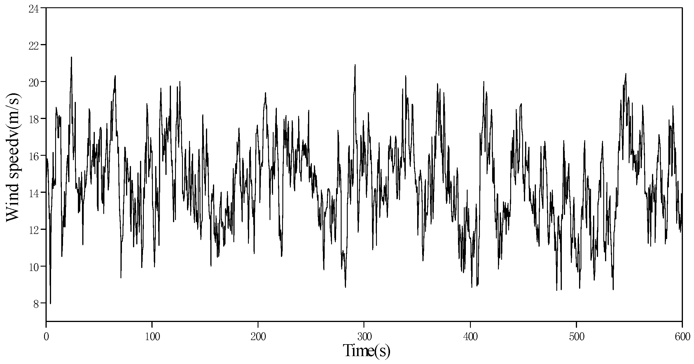
Based on the aforementioned methodology and building upon previous parameter identification approaches, this study employs numerical simulation to generate time series of wind speed. The fundamental parameters used for simulating the pulsating wind field are summarized in

Table 2. Parameters for wind speed time history simulation.

Parameter	Value
Ground Roughness Index	0.12
Ground roughness length/(m)	0.03
Average wind speed at 10 m height/(m/s)	15
Start circular frequency/(rad/s)	0
Frequency Range/(rad/s)	2π
Number of Frequency Points	3000
Time step/s	0.5
Total Simulation Time/s	600

.

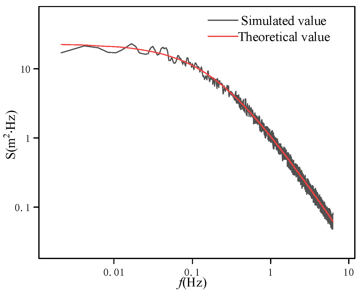
Figure 11 displays the simulated time history of pulsating wind speed, while Figure 12 shows the corresponding power spectral density. The simulated spectrum aligns closely with the target Kaimal spectrum, validating the accuracy of the wind speed simulation. This provides a reliable basis for subsequent dynamic response analyses under wind loading.

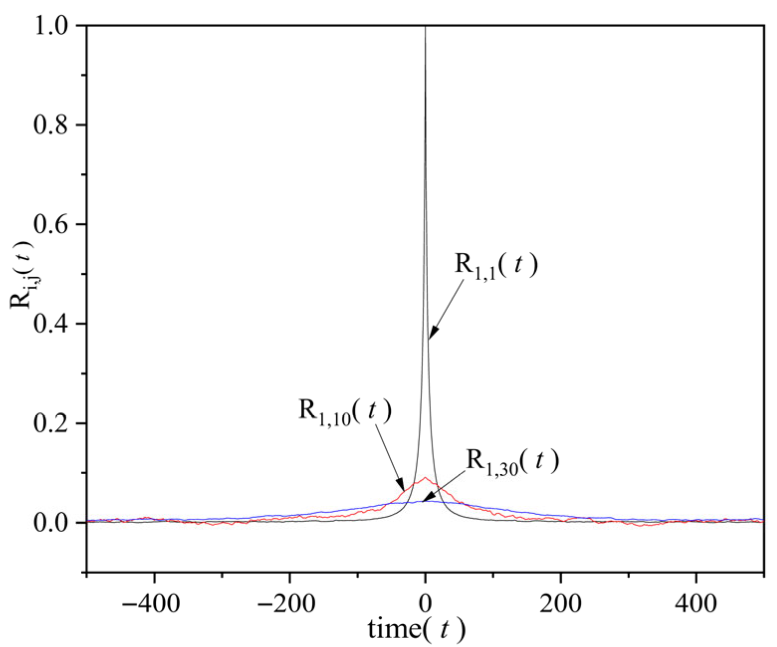
Figure 13 shows the wind speed autocorrelation coefficient R_1,1(t) at the simulated point. As observed in the figure, the value peaks near zero and decreases toward both ends, indicating that the correlation between wind speeds at the same location but different time instances diminishes over time. Additionally, R_1,10(t) represents the cross-correlation between two wind speed simulation points spaced 100 m apart, while R_1,30(t) denotes that for points 300 m apart. A comparison reveals that the correlation weakens as the distance between the simulation points increases. The calculated correlations align with established wind speed behavior, thereby validating the rationality of the simulated wind speeds.

3.2. Wind Deflection Angle Calculation Formula Under Pulsating Wind

This study investigates a high-voltage transmission line with LGJ-400/50 conductors. Relevant operational data indicate a substantial disparity in span lengths between adjacent towers: the span of the 17th conductor measures 1047 m, whereas that of the 18th conductor is only 339 m. A finite element model of this transmission line segment was established, as illustrated in Figure 14.

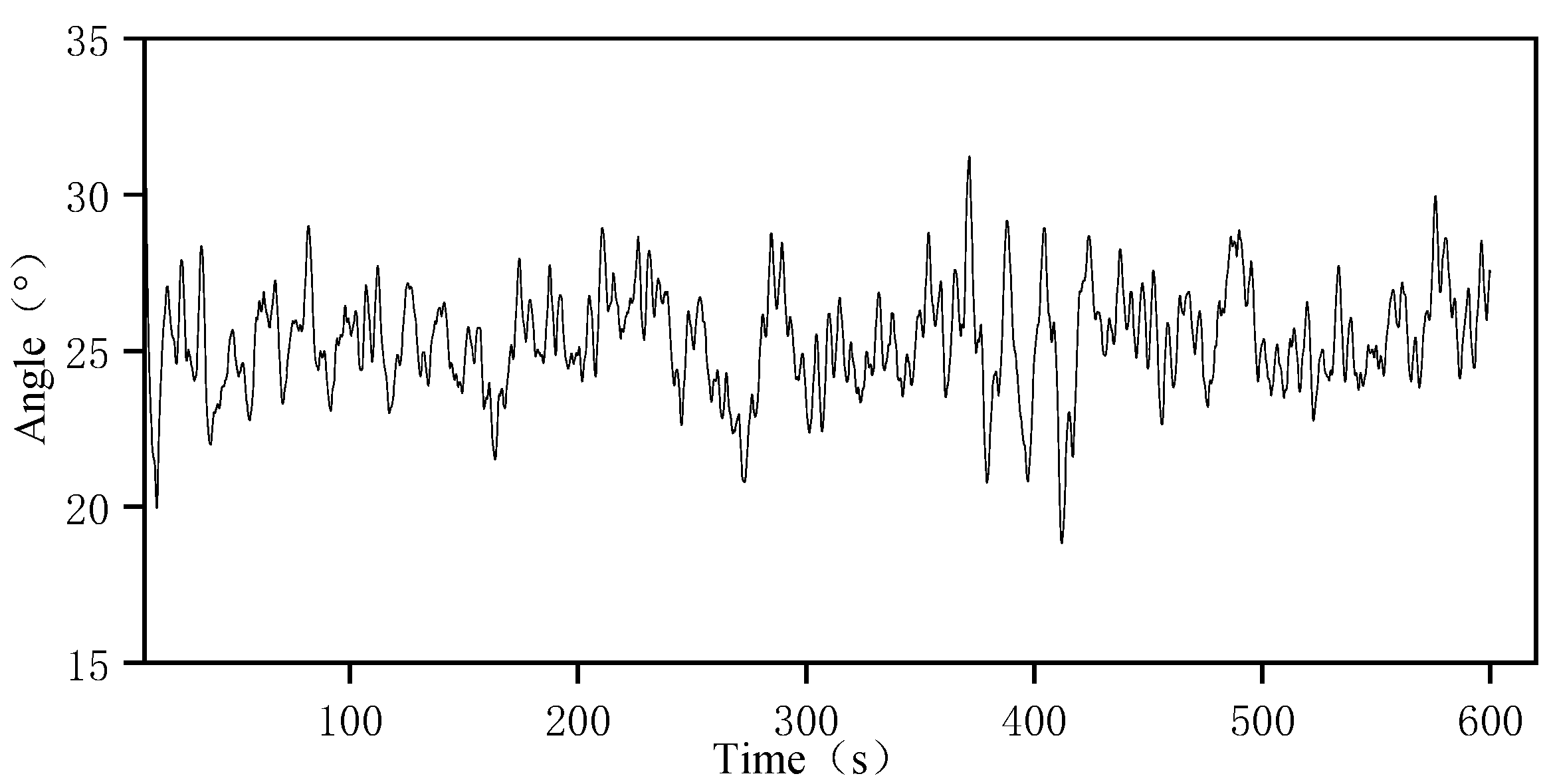
A pulsating wind load with a mean velocity of 25 m/s was applied, featuring a wind attack angle of 90° and a horizontal wind direction angle of 0°. The terrain was selected as Type A-Coastal. Under these conditions, the dynamic deflection curve of the insulator string suspended from the straight tower over a period of 600 s is shown in Figure 15.

As observed in Figure 15, under pulsating wind load, the deflection angle of the insulator string exhibits complex, irregular fluctuations around the mean value. Therefore, considering only the static wind deflection angle or the average deflection under pulsating wind may not sufficiently address the issue of wind-induced flashover in transmission lines. It is essential to fully account for the dynamic characteristics of natural wind to effectively prevent wind deflection flashover accidents.

In practical engineering, the variation in wind deflection due to pulsating wind is commonly described using statistical measures such as the mean and standard deviation, as expressed in Equation (27):

$${\phi }_m=\overline{\phi }+\mu \sigma$$

(27)

where φ_m and $\overline{\phi }$ represent the equivalent deflection angle and the average deflection angle, respectively, μ and σ denote the assurance coefficients and standard deviations, respectively. The assurance coefficient µ reflects the safety margin in structural analysis and varies among countries based on specific regulatory standards. In accordance with national reliability guidelines, the typical value of µ in Chinese standards is approximately 2.2, corresponding to an assurance rate of 98.61%.

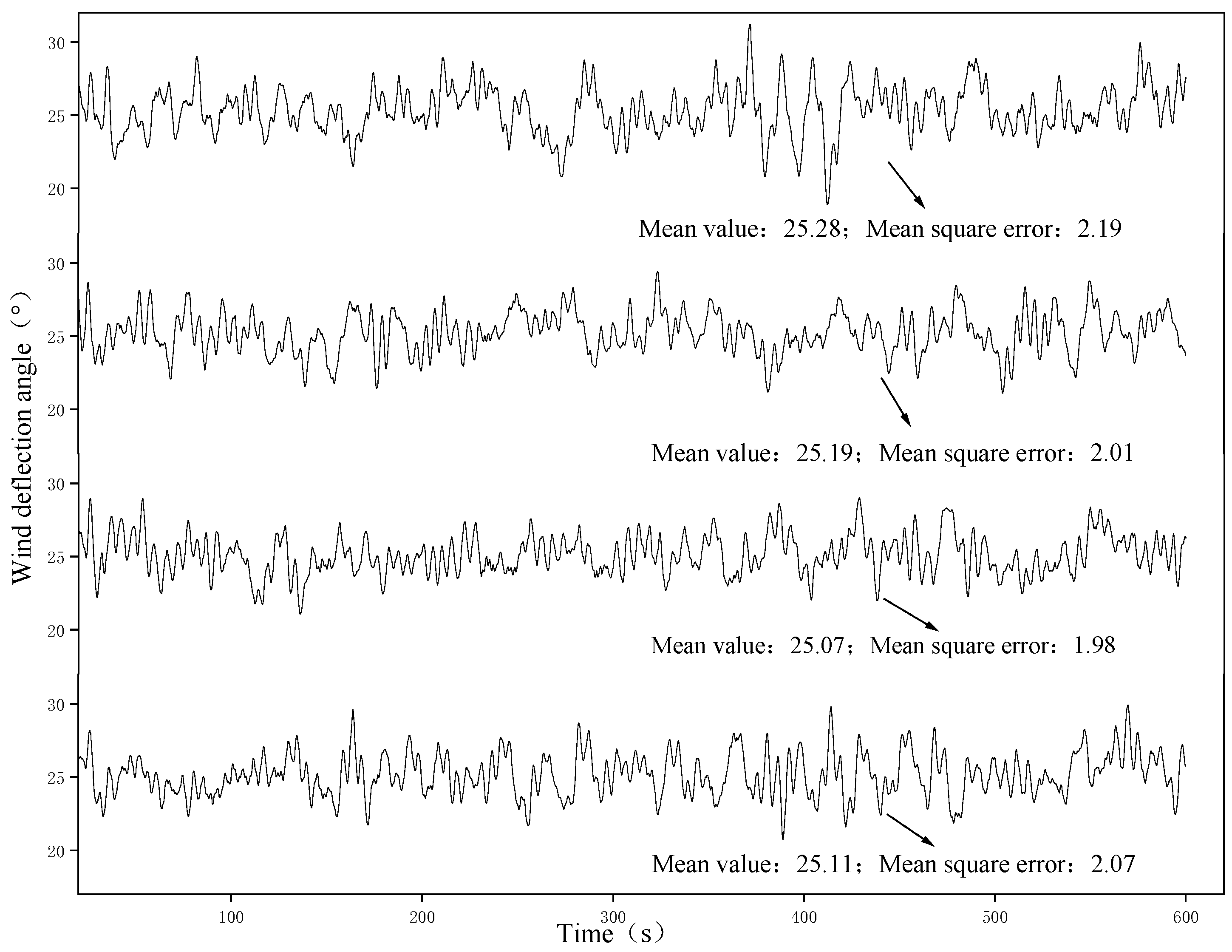
The wind deflection angles of the upper phase insulator string were computed under four sets of stochastic dynamic wind fields, each with a mean wind speed of 25 m/s and a duration of 10 min. The time history curve of the wind deflection angle is presented in Figure 16.

As shown in Figure 16, the mean and variance of wind deflection angles under different pulsating winds exhibit minimal variation, indicating that the results obtained from the proposed model are consistent and effectively eliminate the influence of randomness.

3.3. Effect of Span on Wind Deflection Angle

Based on the actual transmission line configuration shown in Figure 14, the spans on both sides of the straight tower, denoted as L₁ and L₂, were varied from 300 m to 1000 m in increments of 100 m, resulting in 64 working conditions. For cases where the left and right spans are identical, the configuration is symmetric, as illustrated in Figure 17. Theoretically, such symmetric conditions experience identical loads and should yield the same wind deflection angle. Therefore, only one of each symmetric pair was selected for wind deflection analysis.

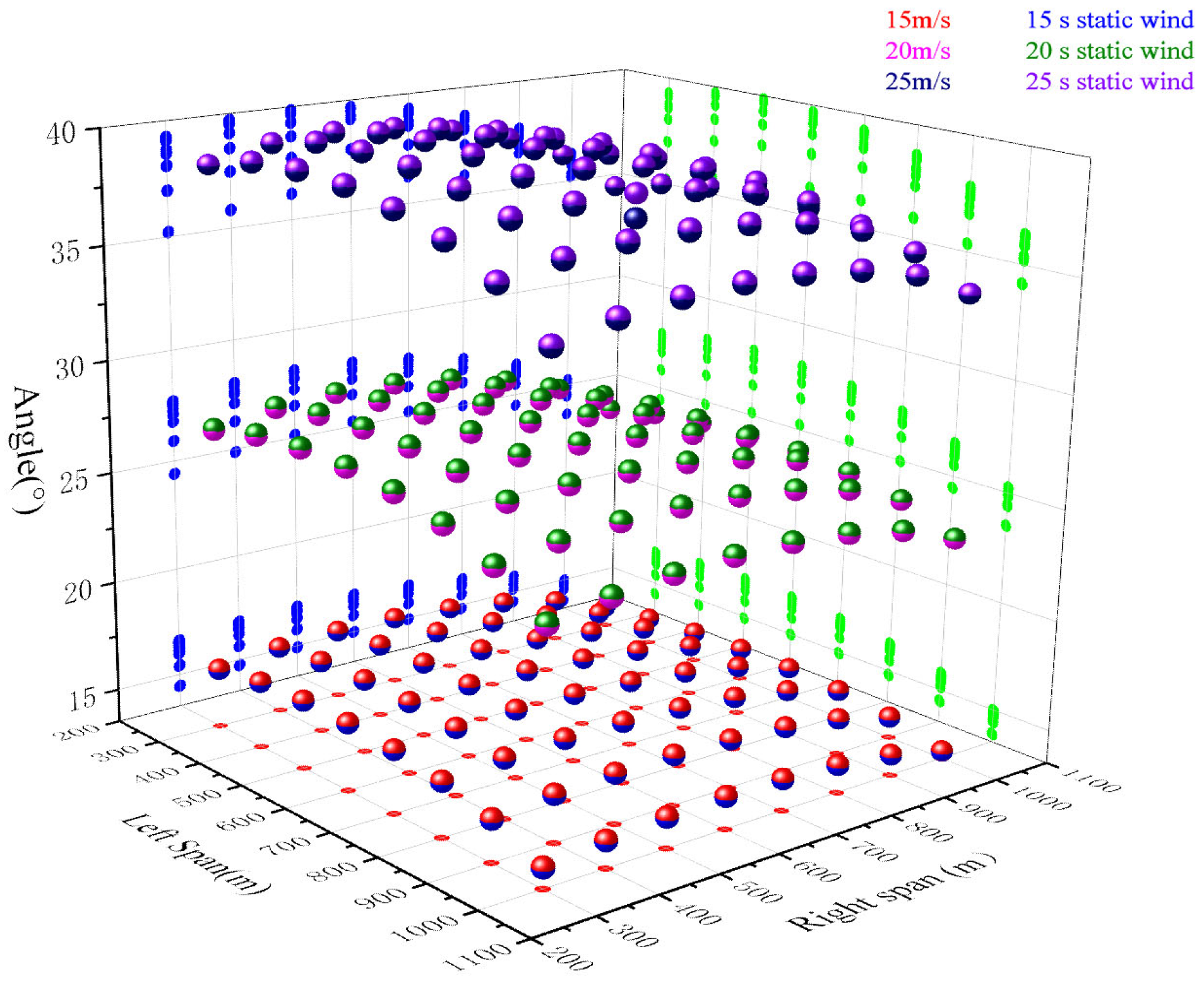
For all considered conditions, wind deflection responses were analyzed under static wind and pulsating wind with average velocities of 15 m/s, 20 m/s, and 25 m/s. Each wind simulation had a duration of 10 min. The corresponding wind deflection angles were statistically evaluated, and the results are presented in Figure 18.

As observed from Figure 18, higher wind speeds lead to a greater wind deflection angle of the suspension insulator string. Moreover, the deflection angle φ under static wind action is approximately equal to the mean deflection angle $\overline{\phi }$ under corresponding pulsating wind action.

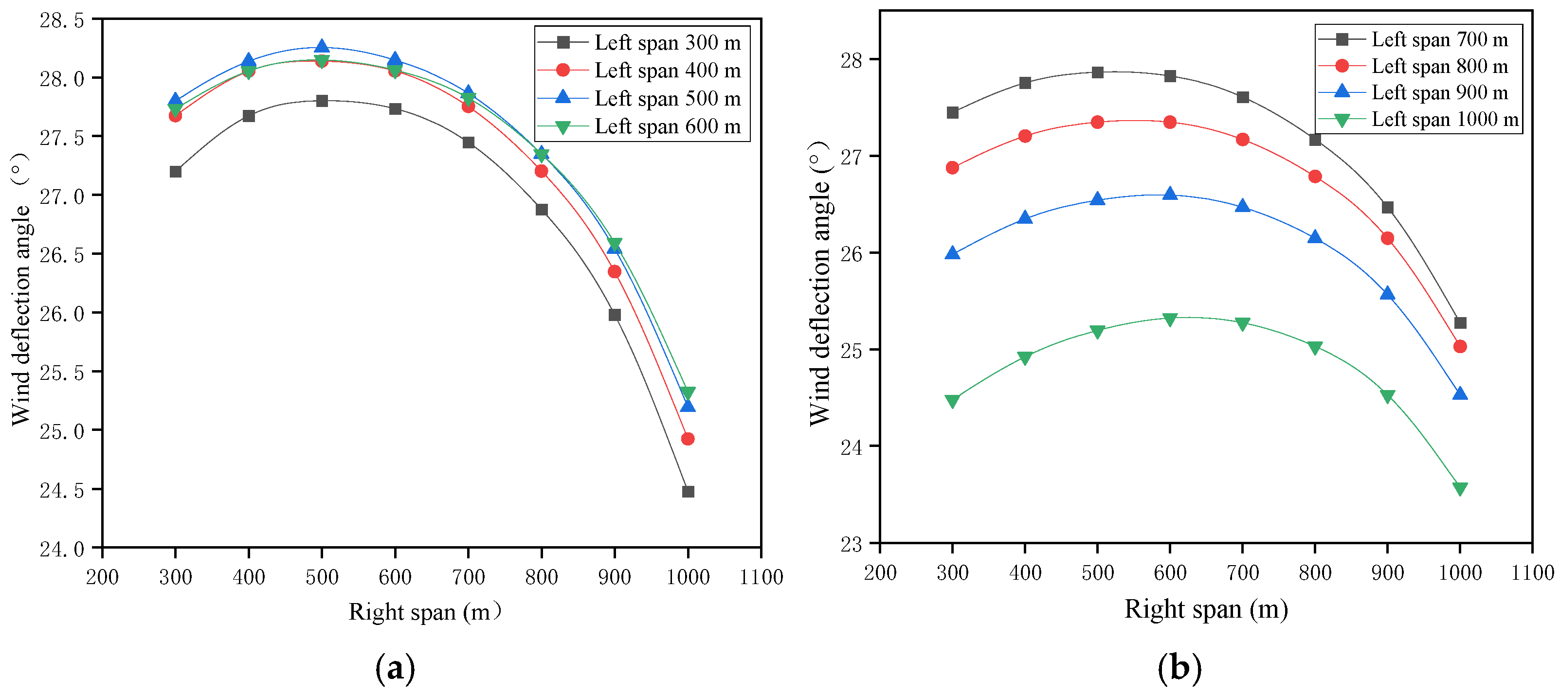
Furthermore, by projecting the scatter points in Figure 18 onto the plane, it can be observed that the variation trend of the wind deflection angle with span remains consistent across different wind speeds. Taking the wind deflection angle under a static wind speed of 20 m/s as an example, the relationship between deflection angle and span is illustrated in Figure 19.

When the span L₁ on one side of the suspension insulator string is held constant, the wind deflection angle initially increases and then decreases as the opposite-side span L₂ increases. This decrease occurs because, under unchanged suspension point height and other sag configuration parameters, a larger span leads to greater mid-span conductor sag (as shown in Figure 17, where the sag is noticeably larger for longer spans). This reduces the clearance between the conductor and the ground or sea level, thereby decreasing the wind pressure height coefficient and consequently the wind load on the conductor. The trend suggests that if the effect of the height coefficient is neglected, the wind deflection angle would increase monotonically with span.

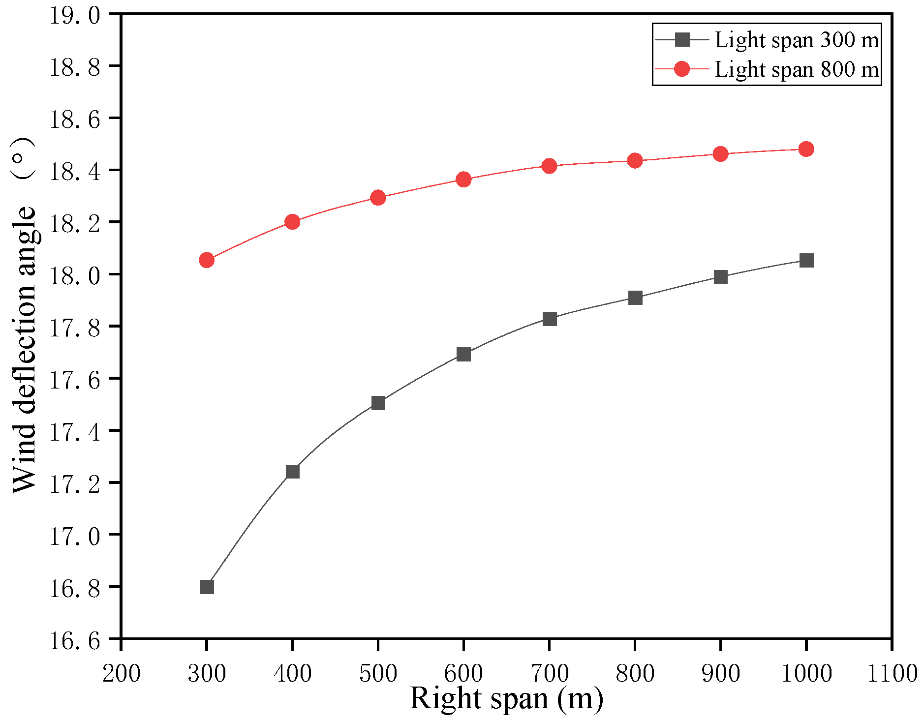
To eliminate the influence of the wind pressure height coefficient in the wind deflection response, the conductor suspension height was set to a fixed reference level. A subset of the working condition models was regenerated, and a static wind speed of 20 m/s was applied for wind deflection analysis. The resulting relationship between wind deflection angle and span, excluding height variation effects, is shown in Figure 20.

It can be observed that when the span on one side of the insulator string is fixed, the wind deflection angle increases continuously with the span on the opposite side, confirming the earlier hypothesis. This behavior occurs because an increase in span L2 leads to a longer conductor length and a larger wind-exposed area, resulting in a greater wind-induced moment. This disrupts the overall torque balance of the system. As the side with increased L2 experiences higher wind load, the system’s center of gravity shifts, leading to an increase in the wind deflection angle.

3.4. Influence of Span on Standard Deviation

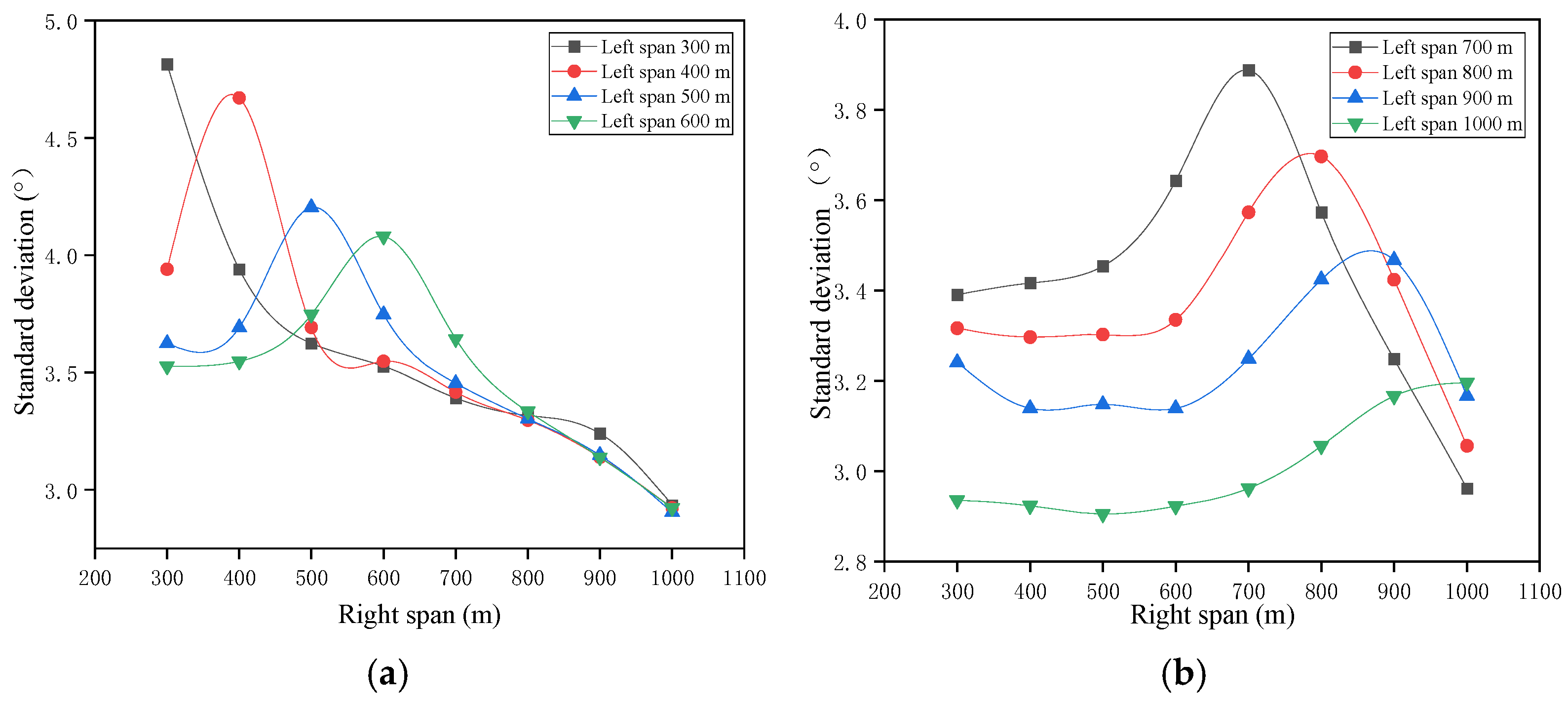
Figure 21 presents the standard deviation σ of wind deflection angle under pulsating wind at 20 m/s for all considered conditions. The results demonstrate that when the left and right span lengths are identical, the standard deviation σ is significantly larger than that under asymmetric span conditions. This is primarily because symmetrical span configurations lead to similar dynamic characteristics in the conductors on both sides, making them prone to synchronous swinging under pulsating wind excitation. This synchronization amplifies the overall amplitude fluctuation of the insulator string, resulting in a larger standard deviation σ of the wind deflection angle. In contrast, when the left and right span lengths differ considerably, the vibration frequencies and phases of the conductors on the two sides vary, leading to non-synchronous swinging. This creates a mutual suppression effect that restrains the overall amplitude development, thereby reducing the standard deviation σ.

Furthermore, under symmetrical span conditions, the standard deviation σ of the wind deflection angle gradually decreases as the span length increases, indicating a more concentrated distribution of the deflection angles. This phenomenon occurs mainly because increased span length leads to greater conductor sag, reducing the height above ground and consequently the wind pressure height coefficient. As a result, the wind load acting on the conductor decreases, which in turn suppresses the fluctuation amplitude of wind-induced vibration.

During the ascending phase, dynamic amplification serves as the governing mechanism. As the span length increases, the vibrational inertia of the conductor under pulsating wind excitation is enhanced. This causes certain natural frequencies of the system to decrease, moving them closer to the high-energy region of the pulsating wind energy spectrum. As a result, a significant dynamic amplification effect is triggered, leading to a pronounced upward trend in the standard deviation.

4. Power Amplification Coefficient

4.1. Dynamic Amplification Under Pulsating Wind

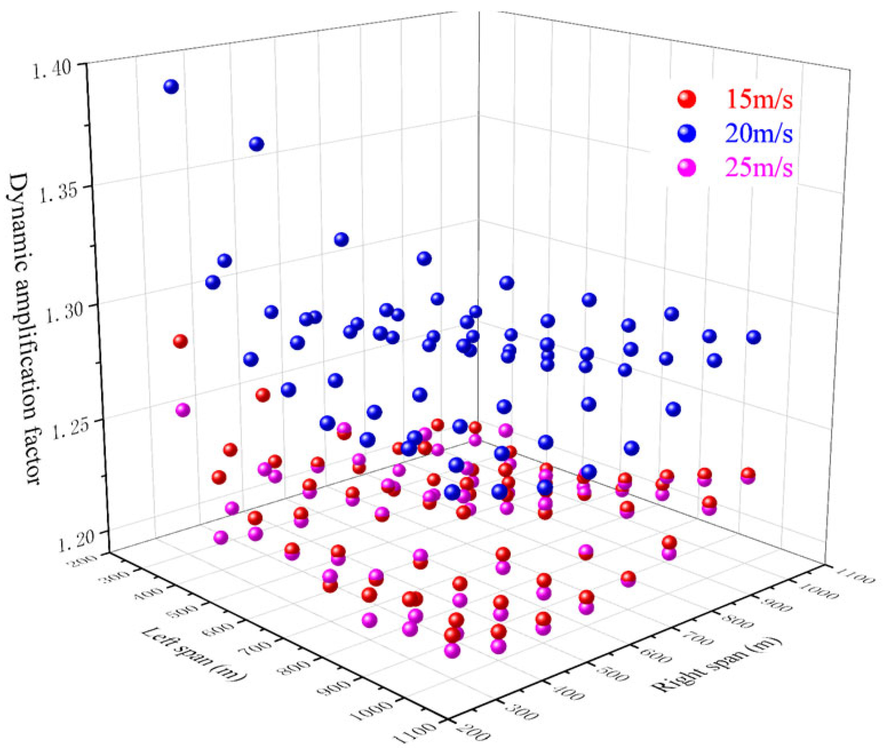
Compared to the wind deflection angle under static wind, the deflection induced by pulsating wind is generally larger. As previously discussed, both the mean value and standard deviation of the wind deflection angle under pulsating wind vary with span length. The dynamic amplification factors for various operating conditions and wind speeds are summarized in Figure 22. These coefficients predominantly fall within the range of 1.2 to 1.35, indicating that dynamic amplification effects must be considered in studies of wind-induced flashover on transmission lines.

At a wind speed of 15 m/s, the dynamic amplification factor for the suspension insulator string ranges between 1.19 and 1.22. When the wind speed increases to 20 m/s, the dynamic amplification factor rises noticeably to between 1.28 and 1.30. However, as the wind speed further increases to 25 m/s, the dynamic amplification factor decreases to approximately 1.20–1.23. This reduction can be attributed to the fact that the equilibrium wind deflection angle of the insulator string increases with wind speed, thereby reducing the relative contribution of pulsating wind deflection to the total deflection angle.

4.2. Polynomial Regression Model for Fitting the Dynamic Amplification Factor

The finite element method faces challenges of substantial computational burden and low efficiency when calculating wind deflection angles. To address this issue, this study employs polynomial fitting to derive a simplified formula. Our objective is to achieve enhanced computational efficiency and improved applicability at the cost of minimal precision loss. Similar to the approach of Wu et al. [37], who utilized machine learning for predicting dynamic responses, this research explores a data-driven path for simplified modeling. Consequently, based on a comprehensive consideration of data characteristics and practical requirements, we select polynomial fitting to establish a lightweight model for coefficient prediction. Based on computed data-including dynamic amplification factor under wind speeds of 15 m/s, 20 m/s, and 25 m/s, and spans ranging from 300 m to 1000 m, the following polynomial model is established:

$$\lambda ={\beta }_0+{\beta }_{1}l+{\beta }_{2}r+{\beta }_3{l}^2+{\beta }_4{r}^2+{\beta }_{5}lr+{\beta }_{6}lv+{\beta }_7{r}^2+{\beta }_{8}rv+{\beta }_9{v}^2$$

(28)

where l, r, and v represent the left span length, right span length, and average wind speed of the pulsating wind, respectively. The model incorporates quadratic and interaction terms to capture potential nonlinear behaviors. By examining the coefficients of the model, we can identify which polynomial terms (such as squared terms of specific variables or interaction terms) contribute most significantly to the predictions. Terms with coefficients approaching zero can be eliminated, thereby yielding a simpler model that is less prone to overfitting.

Using least squares estimation, the parameters in Equation (29) are determined as follows:

$$\begin{array}{c}\lambda =0.31568-0.0001806\cdot (l+r)+0.10966\cdot v+6.55382\times {10}^{-9}\cdot (l^2+r^2)+2.0823\times {10}^{-7}\cdot l\cdot r+\\ 1.02652\times {10}^{-6}\cdot (l+r)\cdot v-0.002785\cdot v^2\end{array}$$

(29)

The rationality and accuracy of this polynomial model require validation through comparison with finite element simulation results. Initially, the reliability of the polynomial will be analyzed using several commonly adopted statistical metrics. The coefficient of determination R² is defined as follows:

$$R^2=1-{\displaystyle \frac{S{S}_{res}}{S{S}_{sot}}}$$

(30)

In the above equation, $S{S}_{res}$ represents the sum of squared residuals, which indicates the variation that the model fails to explain. $S{S}_{res}$ can be expressed as:

$$S{S}_{res}={\displaystyle \sum _{i=1}^n{(y_i-{\widehat{y}}_i)}^2}$$

(31)

In the above formula, $y_i$ represents the calculated value of the i-th finite element. ${\widehat{y}}_i$ is the predicted value calculated based on the fitting formula for the i-th element. $S{S}_{sot}$ is the total sum of squares, which represents the total variation in the dependent variable y itself.

$$S{S}_{sot}={\displaystyle \sum _{i=1}^n{(y_i-\overline{y})}^2}$$

(32)

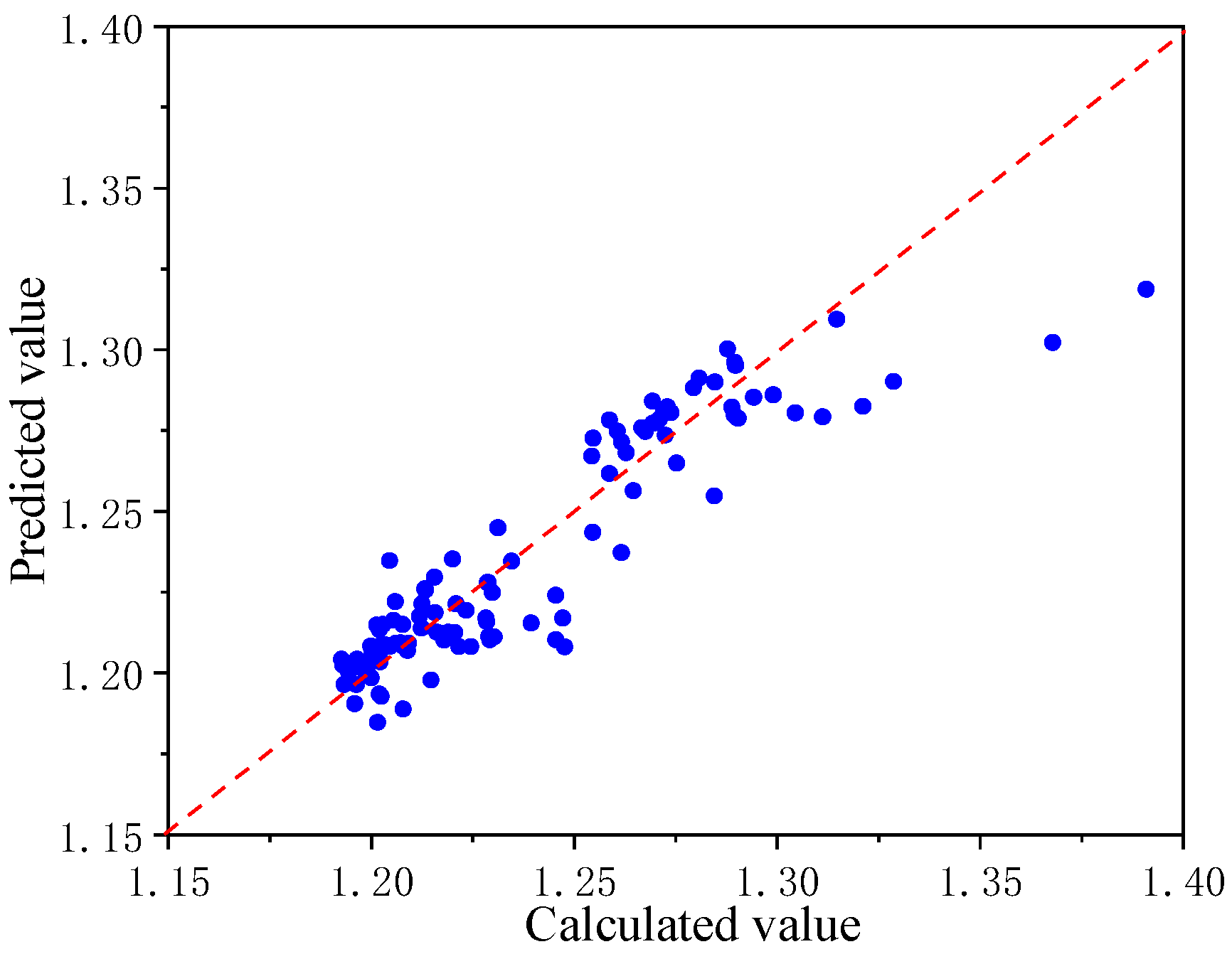
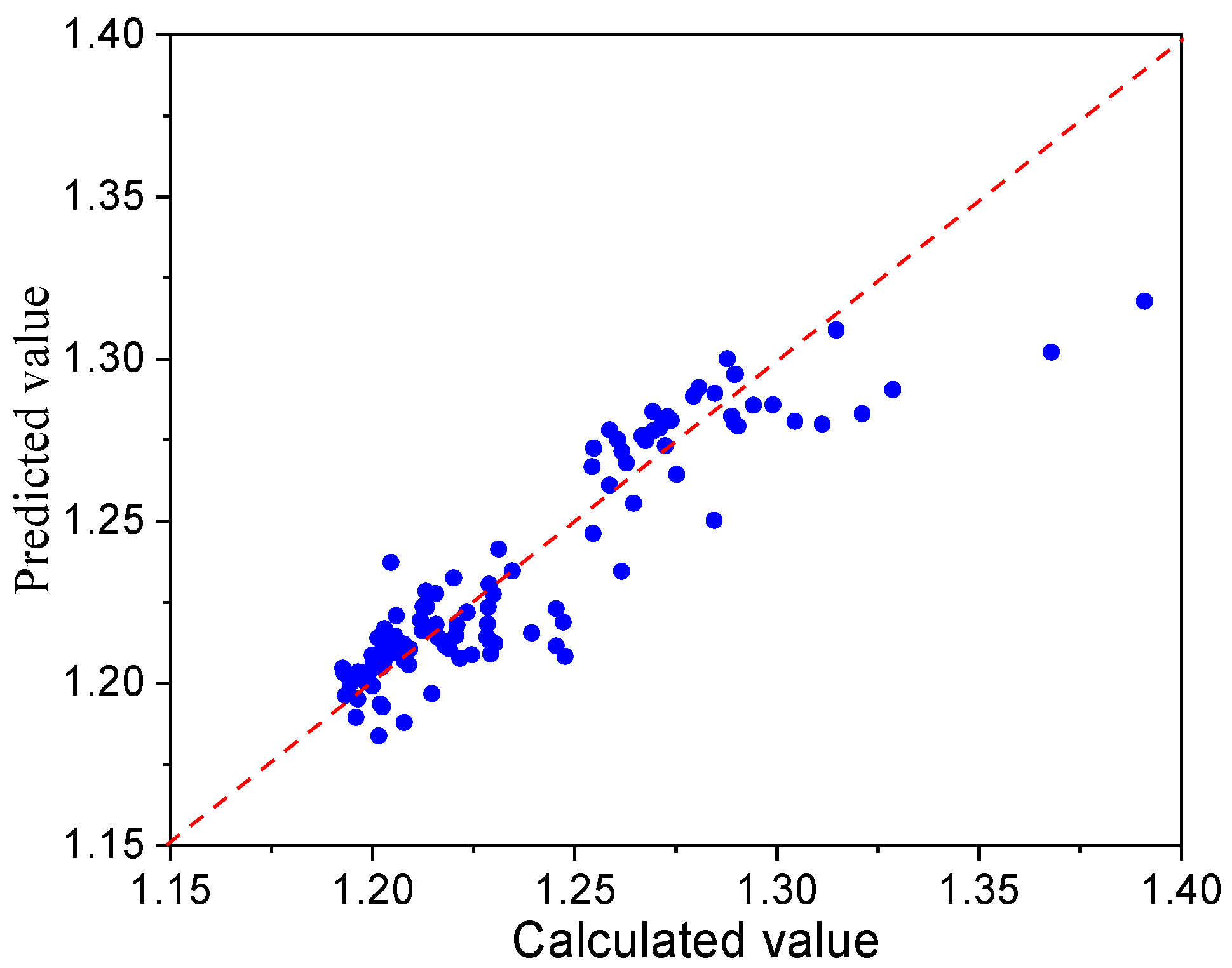
The symbol $\overline{y}$ represents the mean value of all finite element calculation results. Based on the aforementioned formula, the fitting curve presented in the study was analyzed, yielding R² = 0.86, which indicates a strong descriptive capability of the fitting formula. Furthermore, a comparative plot between the predicted values from the formula and the finite element calculation results was generated. The results demonstrate that, with the exception of two data points where the dynamic amplification factor λ exceeds 1.35, the remaining predicted values are uniformly distributed on both sides of the reference line, showing good agreement.

Further examining the percentage error through a scatter plot of discrepancy percentages relative to finite element calculation values, as shown in the following Figure 23:

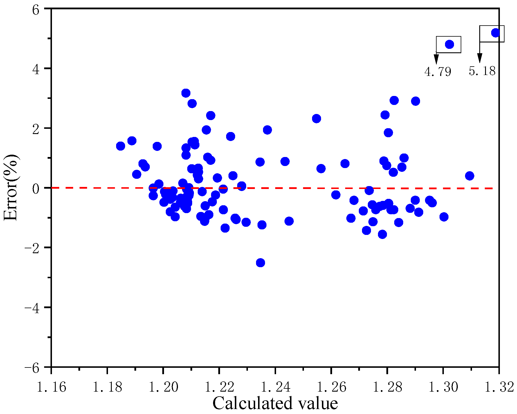
In the Figure 24 above, the vertical coordinate Error (%) represents the percentage error, and its calculation formula is typically expressed as:

$$\mathrm{Error}={\displaystyle \frac{y_i-{\widehat{y}}_i}{y_i}}\times 100\%$$

(33)

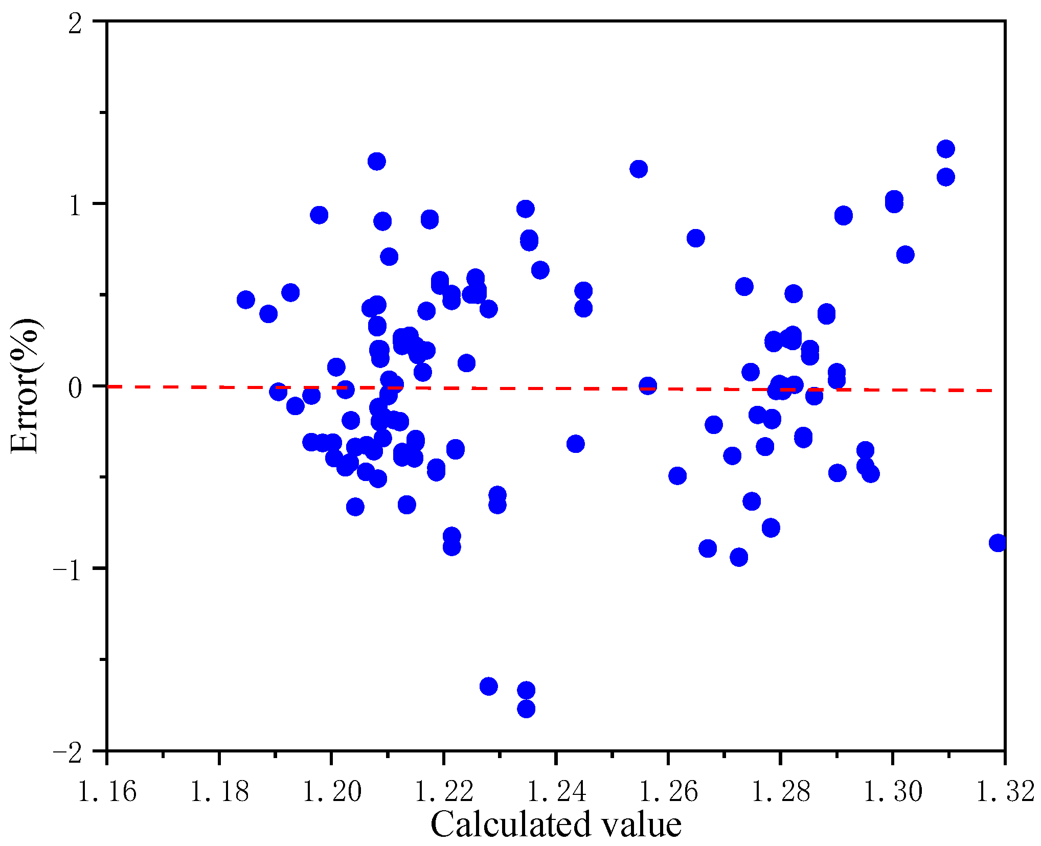
This formula represents the relative deviation of predicted values from the true values. The figure reveals two outliers with significant errors (5.18% and 4.79%, respectively), while all remaining data points exhibit minor deviations, indicating a slight increasing trend in errors with rising λ values.

To further enhance the rationality and accuracy of the fitting formula, PySR was employed for equation acquisition. PySR is a library designed for symbolic regression, which aims to automatically learn mathematical expressions from data through genetic programming. The formula identified by PySR is as follows:

$$\lambda =0.23778+v\left[{\displaystyle \frac{1.4686}{l+0.05728(1.0129r-l)(r-l)-{(-1.2518)}^v}}+(0.10334-0.0026027v)\right]$$

(34)

Based on the above formula, the fitting curve in the text was analyzed, yielding an R² = 0.97. This indicates that the fitting formula possesses a strong descriptive capability and outperforms the polynomial fitting formula.

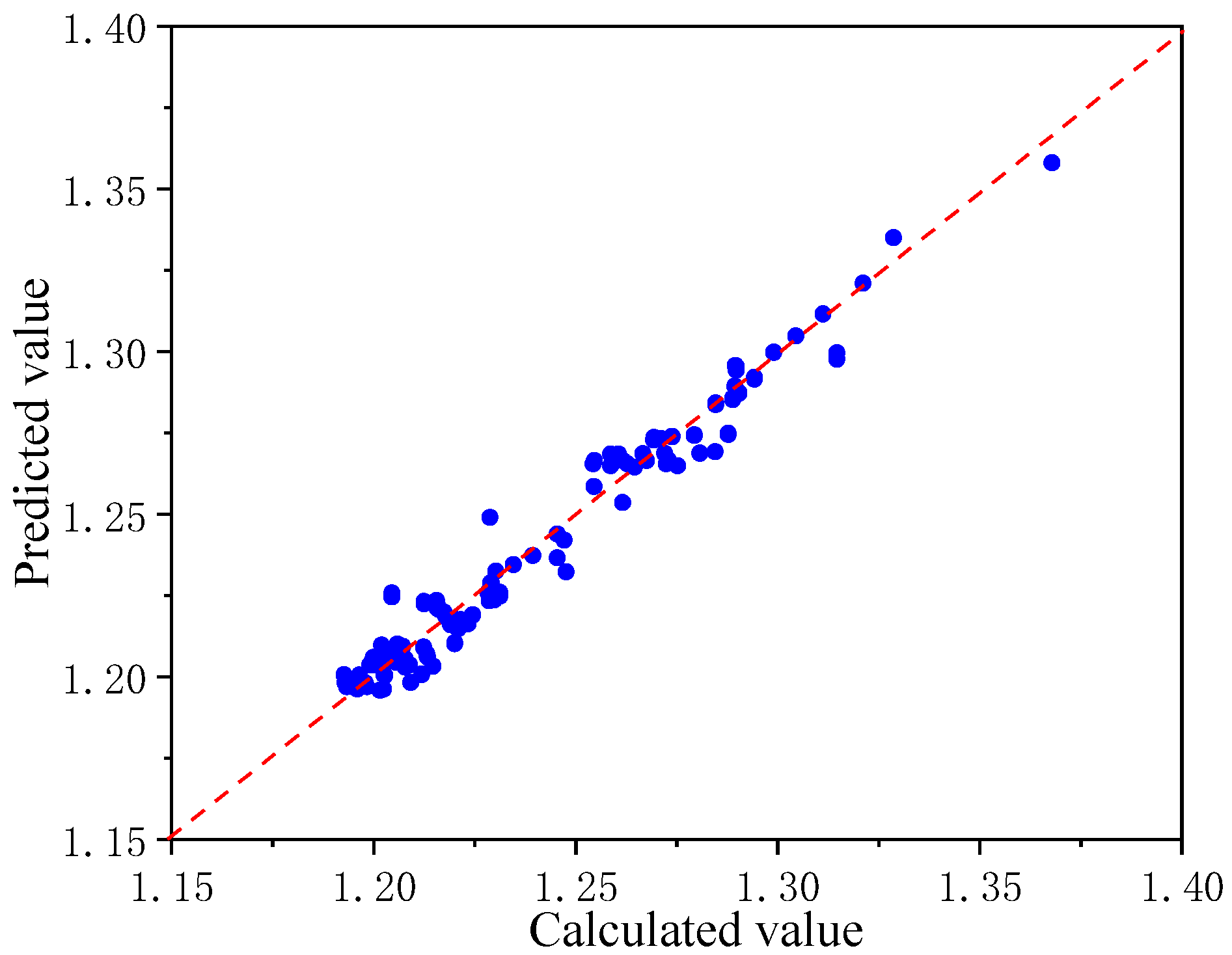
A comparison between the predicted values from the PySR-derived formula and the finite element calculation values is shown in the Figure 25 below. It can be observed that, regardless of the value of λ, the predicted and calculated values are in close agreement, clustering near the reference line.

Based on the PySR-derived formula, the percentage error between the predicted and finite element calculated values is shown in the Figure 26 below. It can be observed that the maximum error is less than 2%, with all data points distributed near the reference line. This indicates that the second formula obtained through PySR, despite its complex form, achieves a high fitting accuracy.

Given the relatively complex form of Equation (33), constraints were applied to the formula derived via PySR logic, favoring a polynomial expression. Consequently, the polynomial form obtained based on PySR logic is presented as follows:

$$\lambda =0.2842+0.11099v-0.0027849v^2-0.00015157(l+r)+2.2082\times {10}^{-7}rl$$

(35)

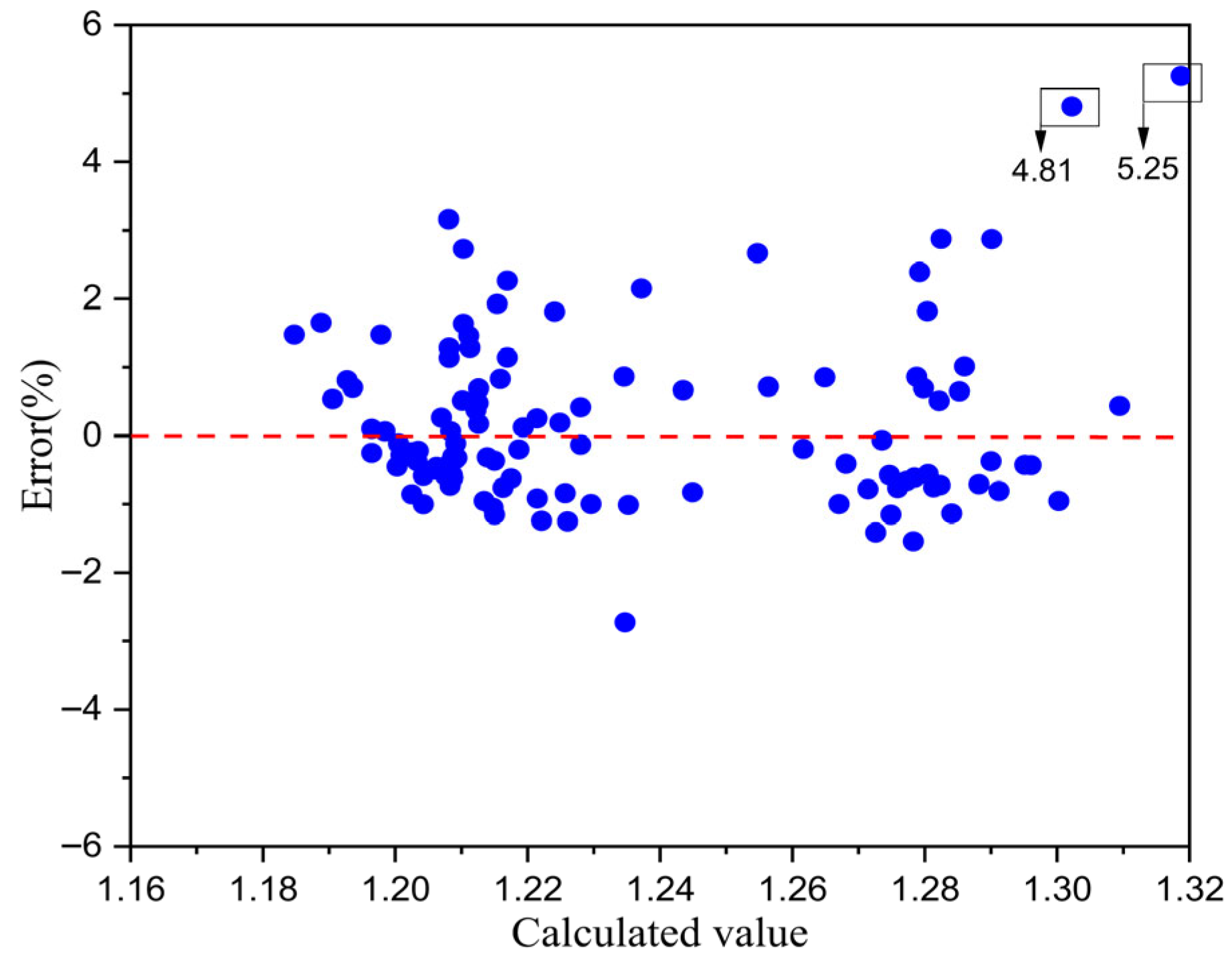
The above equation possesses a simpler form compared to the expression estimated using the least squares method, although the accuracy of both formulations remains comparable. The R² value for this equation reaches 0.86, with Figure 27 presenting the comparison between predicted values and finite element computational results. The corresponding error analysis is shown in Figure 28, revealing a maximum error of 5.25%. By comparing the two polynomial fitting outcomes, it can be observed that despite slightly larger errors, the final expression offers a significantly simpler formulation.

To facilitate practical engineering applications, this subsection attempts to predict finite element simulation results through mathematical formulations, employing both the least squares method and the logical inference method to determine the dynamic amplification coefficient. The research demonstrates that when constrained to polynomial forms, relatively concise expressions can be obtained, though with a maximum error approaching 5%. Conversely, when no restrictions are imposed on the expression form, more accurate results can be achieved, with the maximum error remaining below 2%.

4.3. Engineering Applications

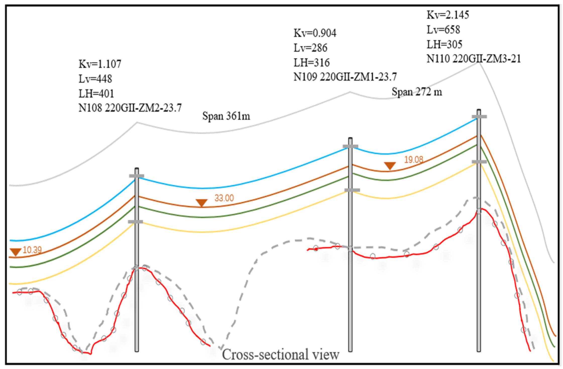
To validate the accuracy of the proposed formula, this section references a fault case model from the 2020 fault trip analysis and mitigation report for a certain 220 kV transmission line, issued by an electric power survey and design institute. A cross-section of the faulted line is shown in Figure 29. The conductor model is JL/G1A-240/30, with a cross-sectional area of A = 5.5 × 10⁻⁴ m, Young’s modulus E = 7.3 × 10⁹ Pa, Poisson’s ratio ν = 0.3, density ρ = 3341 kg/m³, and an axial force at the lowest point of 20 kN. The terrain is classified as Type B (suburban), and the design maximum wind speed for the line is 17 m/s.

Pulsating wind with average wind speeds of 10 m/s, 15 m/s, and 17 m/s were applied to the model, each with a duration of 10 min. The dynamic amplification factor of the wind deflection angle of the suspension insulator string under each wind condition was computed, and the results were compared with predictions from the proposed formula, as summarized in

Table 3. Statistical analysis of insulator string dynamic amplification factor.

Average Wind Speed (m/s)	Steady Wind Deflection Angle (°)	Pulsating Wind Avg. Deflection Angle (°)	Standard Deviation	Dynamic Amplification Factor (Calculated)	Dynamic Amplification Factor (Formula)	Error (%)
13	27.28	27.32	2.25	1.183	1.186	0.3
15	35.80	35.81	3.48	1.214	1.251	3.1
17	45.83	45.85	4.94	1.237	1.293	4.5

.

As shown in Table 3, under varying conductor models, axial forces, and model heights, the discrepancies between the dynamically computed dynamic amplification factors and those predicted by the formula are relatively small. These findings demonstrate that the polynomial regression model established in this study offers high predictive accuracy and practical utility for estimating the dynamic amplification factor across diverse operational scenarios. It can be effectively employed to analyze and predict the dynamic response of suspension insulator strings under various wind speed conditions.

5. Conclusions

Based on the catenary theory, this study obtains the precise initial configuration and internal forces of the conductor, addresses the convergence challenges faced by traditional finite element software when simulating long-span transmission lines. On this basis, self-developed specialized analysis software was employed to systematically investigate the influence of span length on the wind-induced response of suspension insulator strings. The main conclusions are as follows:

(1)

The wind deflection angle under static wind action is essentially consistent with the mean deflection angle under pulsating wind conditions. When the span length on one side of the insulator string is fixed, the deflection angle exhibits a nonlinear trend—first increasing and then decreasing—as the span length on the opposite side increases. If the variation in the wind pressure height coefficient is neglected, the deflection angle would continuously increase with span length.

(2)

Under pulsating wind excitation, symmetrical span configurations amplify the standard deviation of the deflection angle, demonstrating more pronounced fluctuation characteristics. However, under symmetrical span conditions, the standard deviation of the deflection angle gradually decreases as the span length increases, and the equivalent wind-induced deflection angle exhibits a similar trend. This occurs because increased span length leads to greater conductor sag, reduced ground clearance, and consequently a decreased height coefficient. This reduction in the height coefficient diminishes the wind load, thereby suppressing the fluctuation amplitude of the wind deflection angle.

(3)

Pulsating wind exerts a non-negligible dynamic amplification effect on suspension insulator strings. Across various working conditions, the dynamic amplification factor ranges between 1.2 and 1.35, showing a non-monotonic characteristic that first increases and then decreases with rising wind speed.

(4)

Based on symbolic regression and the least squares method, this study derived three distinct expressions for the dynamic amplification factor in terms of span length and wind speed. Accuracy evaluation reveals that the two polynomial expressions obtained through symbolic regression and the least squares method both demonstrate maximum errors approaching 5%, with coefficients of determination (R²) reaching approximately 0.85. This indicates that representing the relationship among span length, wind speed, and dynamic amplification factor using polynomial forms still entails certain deviations. Furthermore, symbolic regression yielded an additional expression with superior goodness-of-fit (R² = 0.97), though characterized by relatively complex formulation. In engineering design, appropriate models can be selected from these alternatives according to specific accuracy requirements. Finally, the rationality and applicability of the proposed predictive formulas were validated through actual engineering case studies.

While the simulation results in this study have undergone rigorous verification against commercial software, certain limitations persist: First, the absence of field-measured response data from actual transmission lines under wind loading conditions prevented more comprehensive experimental validation, suggesting the need for further examination and refinement of the research conclusions. Second, the analysis employed the assumption of wind as a Gaussian stationary random process, with all subsequent analyses and conclusions being conditional upon this premise. Future research should prioritize investigating wind-induced deflection characteristics of transmission lines under non-Gaussian wind field conditions.

References

1. Liu, J.; Ma, H.M.G.; Wang, B.; Cao, L.W.; Chen, C.; Wei, B. Study on the Influence of Wind Profile Coefficient and Turbulence Intensity on Wind Deflection Angle and Tower Head Size Design of Transmission Lines in Tibet. Electr. Eng. 2025, 129–133. [Google Scholar]
2. Man, C.Y.; Man, H.W.; Xie, W. Cause Analysis of Wind Deflection Trip of 220kV II Xiangshan-Suyuan Line. Electr. Eng. 2025, 99–100+104. [Google Scholar]
3. Gu, Y.; Zhang, Y. A Review of Wind-Induced Swing Response Calculations for Transmission Conductors. Eng. Solut. Mech. Mar. 2024, 1, 10. [Google Scholar]
4. Alcayde-García, F.; Salmerón-Manzano, E.; Montero, M.A.; Alcayde, A.; Manzano-Agugliaro, F. Power transmission lines: Worldwide research trends. Energies 2022, 15, 5777. [Google Scholar] [CrossRef]
5. Hileman, A.R. Weather and its effect on air insulation specifications. IEEE Trans. Power Appar. Syst. 1984, PAS-103, 3104–3116. [Google Scholar] [CrossRef]
6. Tsujimoto, K.; Yoshioka, O.; Okumura, T.; Fujii, K.; Simojima, K.; Kubokawa, H. Investigation of conductor swinging by wind and its application for design of compact transmission line. IEEE Trans. Power Appar. Syst. 1982, PAS-101, 4361–4369. [Google Scholar] [CrossRef]
7. Hiratsuka, S.; Matsuzaki, Y.; Fukuda, N.; Yukino, T.; Ishida, H. Field test results of a low wind-pressure conductor. In Proceedings of the IEEE Region 10 International Conference on Electrical and Electronic Technology, Singapore, 19–22 August 2001; IEEE: New York, NY, USA, 2002; Volume 2, pp. 664–668. [Google Scholar]
8. Rikh, V.N. Conductor spacings in transmission lines and effect of long spans with steep slopes in hilly terrain. IE (I) J. 2004, 85, 8–16. [Google Scholar]
9. McClure, G.; Lapointe, M. Modeling the structural dynamic response of overhead transmission lines. Comput. Struct. 2003, 81, 825–834. [Google Scholar] [CrossRef]
10. Yan, B.; Lin, X.; Luo, W.; Chen, Z.; Liu, Z. Numerical study on dynamic swing of suspension insulator string in overhead transmission line under wind load. IEEE Trans. Power Deliv. 2009, 25, 248–259. [Google Scholar] [CrossRef]
11. Diana, G.; Bruni, S.; Cheli, F.; Fossati, F.; Manenti, A. Dynamic analysis of the transmission line crossing “Lago de Maracaibo”. J. Wind. Eng. Ind. Aerodyn. 1998, 74–76, 977–986. [Google Scholar] [CrossRef]
12. An, L.; Guan, Y.; Zhu, Z.; Zhang, R. Research on windage yaw flashovers of transmission lines under wind and rain conditions. Energies 2019, 12, 3728. [Google Scholar] [CrossRef]
13. Liu, Y.; Guo, Y.; Wang, B.; Li, Q.; Gao, Q.; Wan, Y. Research on Influencing Factors and Wind Deflection Warning of Transmission Lines Based on Meteorological Prediction. Energies 2024, 17, 2612. [Google Scholar] [CrossRef]
14. Li, J.X.; McClure, G.; Wang, S.H. Ensuring the structural safety of overhead transmission lines by design. J. Aerosp. Eng. 2021, 34, 04021010. [Google Scholar] [CrossRef]
15. Song, P.; Lang, X.; Zhang, S.; Yang, B.; Zhang, S.; Rong, K.; Tian, L. Study on windage response suppression of large-span transmission tower-line system using a spring-pendulum dynamic vibration absorber. Energies 2024, 17, 5638. [Google Scholar] [CrossRef]
16. Chen, X.; Han, M.; Yang, X.; Wang, B. Stability Analysis of Parametric Vibration in Overhead Conductors Under Time-Varying Tension. Symmetry 2025, 17, 464. [Google Scholar] [CrossRef]
17. Zhao, S.; Yue, J.; Savory, E.; Yan, Z.; Chen, J.; Zhang, B.; Peng, L. Dynamic windage yaw angle and dynamic wind load factor of a suspension insulator string. Shock Vib. 2022, 2022, 6822689. [Google Scholar] [CrossRef]
18. Tripathi, A.N.; Verma, A.R. Assessment of Voltage and E-Field Distribution in Outdoor Composite Insulator in 500 kV System for Interface Defects. In Proceedings of the 2023 4th International Conference on High Voltage Engineering and Power Systems (ICHVEPS), Denpasar Bali, Indonesia, 6–10 August 2023; IEEE: New York, NY, USA, 2023; pp. 304–308. [Google Scholar]
19. Bao, H.; Xia, L.; Chai, S.; Cheng, Y.; Cao, S.; Lan, Z. Nonlinear Buckling Analysis and Optimization Design of the Y-Type Composite Insulator String. Adv. Civ. Eng. 2022, 2022, 4398388. [Google Scholar] [CrossRef]
20. Fatima, K.; Shareef, H. Dynamic Bayesian Network Model for Overhead Power Lines Affected by Hurricanes. Forecasting 2025, 7, 11. [Google Scholar] [CrossRef]
21. Goulioti, E.G.; Nikou, T.Μ.; Kontargyri, V.T.; Christodoulou, C.A. Smart-Grid Technologies and Climate Change: How to Use Smart Sensors and Data Processing to Enhance Grid Resilience in High-Impact High-Frequency Events. Energies 2025, 18, 2793. [Google Scholar] [CrossRef]
22. Snaiki, R. Performance-based ice engineering framework: A data-driven multi-scale approach. Cold Reg. Sci. Technol. 2024, 224, 104247. [Google Scholar] [CrossRef]
23. Zhao, S.; Zhang, X.; Zhang, C.; Yan, Z.; Zhang, X.; Zhang, B.; Dai, X. Extreme-Value Combination Rules for Tower–Line Systems Under Non-Gaussian Wind-Induced Vibration Response. Buildings 2025, 15, 1871. [Google Scholar] [CrossRef]
24. Hou, H.; Zhang, Z.; Yu, J.; Wei, R.; Huang, Y.; Li, X. Damage prediction of 10 kV power towers in distribution network under typhoon disaster based on data-driven model. Int. J. Electr. Power Energy Syst. 2022, 142, 108307. [Google Scholar] [CrossRef]
25. Qian, T.; Xie, Z.; Shi, W.; Shi, Z.; Tan, L. Investigation on the flow field characteristics of composite insulators under extreme wind loads. Eng. Fail. Anal. 2021, 129, 105699. [Google Scholar] [CrossRef]
26. Qian, X.; Gao, Z.; Wang, T.; Wang, L.; Ke, S. Nonlinear aeroelastic response analysis of 100-meter-scale flexible wind turbine blades. Acta Aerodyn. Sin. 2022, 40, 220–230. [Google Scholar]
27. Tian, C.; Tan, Z.Q.; Lu, X.L. Analysis of Wind Vibration Response of Large—Span Asymmetric Suspension Structures with Series Inerter Dampers. Appl. Math. Mech. 2025, 46, 310–323. [Google Scholar]
28. Lou, W.-J.; Zhang, Y.-L.; Xu, H.-W.; Huang, M.-F. Jump height of an iced transmission conductor considering joint action of ice-shedding and wind. Cold Reg. Sci. Technol. 2022, 199, 103576. [Google Scholar] [CrossRef]
29. Huang, G.; Yan, B.; Guo, Y.; Zhang, B.; Wu, G. Experimental study on dynamic response characteristics of isolated-span transmission lines after ice-shedding. High Volt. 2023, 8, 196–208. [Google Scholar] [CrossRef]
30. Lu, J.; Wang, J.; Lu, Z.; Huang, Z.; Fan, L.; Wu, C.; Liu, X. Research on icing four-split wire-induced de-icing algorithm based on CR method. Chinese Journal of Computational Mechanics. Chin. J. Comput. Mech. 2024, 6, 1116–1123. [Google Scholar]
31. Cai, S.; Liu, K.; Long, S.; Shen, P. Co-Rotational procedure for geometric non-linear finite element method of space truss. In Proceedings of the 13th National Conference on Structural Engineering (Volume I), Jinggangshan, China, 16–18 October 2004; Tsinghua University Press: Beijing, China, 2004; pp. 251–255. [Google Scholar]
32. Chen, Z.T.; Fan, Q.S.; Wu, H.Y. Nonlinear motion analysis on 500kV compact line conductor. J. Tsinghua Univ. (Sci. Technol.) 1999, 12, 101–104. [Google Scholar]
33. Crisfield, M.A.; Tassoulas, J.L. Non-Linear Finite Element Analysis of Solids and Structures: Essentials. J. Eng. Mech. 1993, 119, 1504–1505. [Google Scholar] [CrossRef]
34. Belytschko, T.; Liu, W.K.; Moran, B.; Elkhodary, K. Nonlinear Finite Elements for Continua and Structures; John Wiley & Sons Inc.: Hoboken, NJ, USA, 2014. [Google Scholar]
35. Wei, S.T.; Zhao, C.; Sun, Q. Investigating the non-Gaussian property and its influence on extreme wind pressures on the long-span cylindrical roof. Appl. Sci. 2023, 13, 7691. [Google Scholar] [CrossRef]
36. Yang, Q.; Zhou, T.; Yan, B.; Liu, M.; Van Phuc, P.; Shu, Z. LES study of topographical effects of simplified 3D hills with different slopes on ABL flows considering terrain exposure conditions. J. Wind. Eng. Ind. Aerodyn. 2021, 210, 104513. [Google Scholar] [CrossRef]
37. Wu, K.; Yan, B.; Yang, H.; Lu, J.; Xue, Z.; Liang, M.; Teng, Y. Dynamic Response Characteristics of Isolated-Span Transmission Lines After Ice-Shedding. Power Deliv. IEEE Trans. (T-PWRD) 2023, 38, 12. [Google Scholar] [CrossRef]
Figure 1. Geometric relationships and internal forces of space truss elements.
Symmetry 17 01968 g001
Figure 2. Schematic diagram of the catenary.
Symmetry 17 01968 g002
Figure 3. Schematic diagram of the three-span conductor line structure.
Symmetry 17 01968 g003
Figure 4. Static balance displacement cloud of the conductor obtained from ABAQUS.
Symmetry 17 01968 g004
Figure 5. Comparison of midpoint displacement time history under non-damped conditions.
Symmetry 17 01968 g005
Figure 6. Comparison of midpoint displacement time histories under damped conditions.
Symmetry 17 01968 g006
Figure 7. Calculated results corresponding to different α coefficients.
Symmetry 17 01968 g007
Figure 8. Calculated results for different numbers of elements.
Symmetry 17 01968 g008
Figure 9. Influence of the convergence tolerance η on the computational results.
Symmetry 17 01968 g009
Figure 10. The impact of time increment (Δt) on computational accuracy and efficiency.
Symmetry 17 01968 g010
Figure 11. Simulated pulsating wind speed time history.
Symmetry 17 01968 g011
Figure 12. Comparison between simulated and target wind spectra.
Symmetry 17 01968 g012
Figure 13. Correlation functions among typical wind speed simulation points.
Symmetry 17 01968 g013
Figure 14. Finite element model of the actual transmission line.
Symmetry 17 01968 g014
Figure 15. Time-domain wind deflection angle of the suspension insulator string on the transmission tower.
Symmetry 17 01968 g015
Figure 16. Time history of wind deflection angle for the suspension insulator string under different wind fields.
Symmetry 17 01968 g016
Figure 17. Schematic of working condition with equal left and right spans.
Symmetry 17 01968 g017
Figure 18. Finite element calculation results of wind deflection under different span conditions.
Symmetry 17 01968 g018
Figure 19. Finite element calculation results of wind deflection under static wind at 20 m/s for varying right-side spans. (a) Wind deflection angle for left span ranging from 300 to 600 m. (b) Wind deflection angle for left span ranging from 700 to 1000 m.
Symmetry 17 01968 g019
Figure 20. Change of span-wind deflection angle ignoring height coefficient.
Symmetry 17 01968 g020
Figure 21. Standard deviation of the wind deflection angle under pulsating wind for varying right-span configurations. (a) Standard deviation σ of the wind deflection angle for a left span from 300 to 600 m. (b) Standard deviation σ of the wind deflection angle for a left span of 700–1000 m.
Symmetry 17 01968 g021
Figure 22. Dynamic amplification factor under various wind speeds and operating conditions.
Symmetry 17 01968 g022
Figure 23. Comparative Plot of Formula-Predicted Values versus Finite Element Calculation Results.
Symmetry 17 01968 g023
Figure 24. Scatter Plot of Percentage Error versus Calculated Values.
Symmetry 17 01968 g024
Figure 25. Comparison between Predicted Values from the PySR-derived Formula and Finite Element Calculation Values.
Symmetry 17 01968 g025
Figure 26. Scatter Plot of Percentage Error from PySR versus Calculated Values.
Symmetry 17 01968 g026
Figure 27. Comparison between Predicted Values from the PySR-derived Formula and Finite Element Calculation Values.
Symmetry 17 01968 g027
Figure 28. Scatter Plot of Percentage Error from PySR versus Calculated Values.
Symmetry 17 01968 g028
Figure 29. Accident section diagram.
Symmetry 17 01968 g029