Mechanical Parameter Identification of Permanent Magnet Synchronous Motor Based on Symmetry

Abstract

Permanent Magnet Synchronous Motors (PMSMs) have been widely applied across various electrical systems due to their significant advantages, including high power density, high-efficiency conversion, and easy controllability. However, the issue of ‘parameter asymmetry’ (a mismatch between the controller’s preset parameters and the actual system parameters) in PMSMs can lead to performance problems, such as delayed speed response and increased overshoot. The destruction of symmetry, including the asymmetric weight distribution between new and old data in the moment-of-inertia identification algorithm and the asymmetry between “measured values and true values” caused by sampling delay, is the core factor limiting the system’s control performance. All these factors significantly affect the accuracy of parameter identification and the system’s stability. To address this, this study focuses on the mechanical parameter identification of PMSMs with the core goal of “symmetric matching between set values and true values”. Firstly, a current-speed dual closed-loop vector control system model is constructed. The PI parameters are tuned to meet the symmetric tracking requirements of “set value-feedback” in the dual loops, and the influence of the PMSM’s moment of inertia on the loop symmetry is analyzed. Secondly, the symmetry defects of traditional algorithms are highlighted, such as the imbalance between “data weight and working condition characteristics” in the least-squares method and the mismatch between “set inertia and true inertia” caused by data saturation. Finally, a Forgetting Factor Recursive Least Squares (FFRLS) scheme is proposed: the timing asymmetry of signals is corrected via a first-order inertial link, a forgetting factor λ is introduced to balance data weights, and a recursive structure is adopted to avoid data saturation. Simulation results show that when λ = 0.92, the identification accuracy reaches +5% with a convergence time of 0.39 s. Moreover, dynamic symmetry can still be maintained under multiple multiples of inertia, thereby improving identification performance and ensuring symmetry in servo control.

1. Introduction

1.1. Research Background and Significance

The servo system of a PMSM consists of a servo driver, a motor, and mechanical transmission components. It is a closed-loop system for precise speed and torque control and is widely used in high-end fields such as aerospace and industrial robotics. During actual operation, system parameters (e.g., moment of inertia, load torque) are prone to changes in working conditions, leading to “parameter asymmetry”—a mismatch between the controller’s preset parameters and the system’s actual parameters. This mismatch causes problems such as delayed speed response and increased overshoot. For example, changes in the load on an electric vehicle can alter the drive shaft’s moment of inertia; if the controller fails to adapt in real time, the accuracy of speed regulation will be reduced. Fluctuations in load torque disrupt the balance and symmetry between electromagnetic and load torque, thereby affecting the system’s stability.

Symmetry, as an important characteristic of control systems, is reflected in the balanced matching between the system’s input and output, as well as between parameter settings and actual operating conditions. In the speed loop control of PMSMs, the destruction of symmetry is a core factor restricting performance: on the one hand, if the moment of inertia identification algorithm assigns asymmetric weights to new and old data, the identification result will deviate from the actual value; on the other hand, the sampling delay causes a deviation between the measured signal and the actual state, resulting in asymmetry between the “sampled value and the true value”. Therefore, optimizing the mechanical parameter identification algorithm based on symmetry principles has significant engineering value for improving the control performance of PMSMs.

1.2. Research Status

1.

Model Reference Adaptive System

The core idea of the Model Reference Adaptive System (MRAS) algorithm is to set a reference model and compare the output of the system to be identified with that of the reference model. Based on the comparison, the generated error is used to construct an adaptive correction law to identify and control system parameters. This entire process is carried out continuously, enabling the value to gradually approach or track the output value of the reference model.

Literature [1] proposes a distributed model reference adaptive control (D-MRAC) scheme, which does not involve the explicit disturbance observers or internal model units. This not only enhances the system’s robustness but also improves its transient performance. Even when the system is subjected to exogenous disturbances, this algorithm can realize online identification and adaptive control of various parameters. This new parameter identification method avoids complex model analysis and simplifies parameter identification and corresponding control strategies, thereby enhancing the system’s stability and robustness. Literature [2] introduces a model-reference adaptive system with nonlinearly adjusted adaptive gain. Based on changes in servo system speed and torque differences, this method can determine whether the system is subject to external disturbances and adjust the adaptive gain accordingly. Literature [3] adjusts the adaptive gain using the power function method, enabling the system to maintain high-accuracy inertia identification even when load torque changes frequently and enhancing the robustness and practical value of the identification system.

The advantage of this algorithm lies in its real-time identification and control of system parameters via the reference model’s output and adaptive correction, thereby improving the system’s adaptability and accuracy. However, this algorithm is highly dependent on model accuracy, leading to limited identification performance when the parameter model differs significantly from the actual system. Moreover, its adjustment speed is slow when facing a dynamically changing environment with rapid variations. In addition, the adaptive algorithm requires complex calculations and substantial computing resources.

2.

State Observer

The parameter identification algorithm based on a state observer achieves accurate parameter identification primarily through real-time state observer observation and parameter adjustment. Its key lies in appropriately adjusting the observer gain to maintain observation accuracy and system stability. The algorithm’s complexity increases with the system’s order; therefore, in practical applications, the system’s complexity and practicality should be fully considered to achieve an optimal balance between performance and computational complexity.

A finite-time extended state observer is proposed in Literature [4]. In contrast to traditional extended state observers, this approach enables the estimation error to converge to zero in finite time, thereby achieving faster convergence and more precise estimates. A disturbance observer is employed in the Literature [5] to assess the external disturbances acting on the system. Subsequent calculations based on the mechanical equation allow for the acquisition of the moment of inertia’s identified value. The findings indicate that the moment of inertia obtained via this approach exhibits outstanding tracking performance and a tiny error margin. In Literature [6], a reduced-order extended Luenberger observer is utilized; meanwhile, the effectiveness of the proposed algorithm—specifically in identifying the moment of inertia of motor drive systems under low-speed operating conditions—is validated through both simulation and experimental means.

3.

Intelligent Identification Algorithm

Literature [7] uses a dynamic self-learning particle swarm optimization (PSO) algorithm to estimate motor parameters. This algorithm performs excellently at tracking multiple parameters and has achieved good results, as verified by experiments. Literature [8] proposes a PPFNN with asymmetric membership functions, which is applied to the inertia identification of PMSMs. Literature [9] designs an interconnected extended sliding mode observer (IESMO). The innovation of this method lies in considering the dynamic coupling relationship between load torque and moment of inertia simultaneously, rather than identifying them in isolation. The observer suppresses disturbances by leveraging the inherent robustness of sliding-mode variable-structure control, thereby achieving faster response and higher accuracy during dynamic processes.

4.

Least Squares Method

Gauss first introduced the Least Squares Method (LSM) and was initially used to analyze the orbital paths of planets. When applied to moment of inertia identification, its core idea is to use the linearized motor model and data samples collected during real-time system operation to adjust previous estimates and minimize the sum of squared differences between the actual and calculated outputs. When this difference is minimized, the parameter identification process is complete. Due to the small number of parameters in the equivalent model, as well as the LSM’s advantages of quick convergence during the identification process, derivative algorithms based on the LSM are widely used in system parameter identification [10].

Literature [11] adopts the LSM for parameter identification. While its principle is simple and easy to implement, it has drawbacks such as a large data processing volume (requiring storage of all historical data) and identification accuracy that is easily affected by input data. To address the problem of massive input data, the RLS method is usually introduced for parameter identification. Literature [12] uses the RLS method, which does not require a complete recalculation for each new input; instead, it updates the model with new data, thereby improving computational efficiency. However, during identification, the RLS method tends to place greater weight on new data while neglecting historical data [13,14,15].

The advantages of the LSM lie in its simple principle and ease of practical operation. After linearizing the motor model and sampling real-time data, the algorithm gradually fine-tunes previous estimates, minimizes the sum of squared errors between actual and estimated outputs, and converges quickly. Compared with other algorithms, the LSM generally shows strong robustness to noisy data, effectively filtering out noise and yielding reliable parameter estimates [16,17,18,19,20]. However, in practical applications, it may require additional methods to handle nonlinear systems, and appropriate solutions are also needed to address the memory consumption issue that may arise from historical data processing. Therefore, this paper conducts in-depth research to address the problems identified in the aforementioned studies, focusing on improving identification accuracy and convergence speed. The main work of this article is:

(1) Construct a current-speed dual closed-loop vector control system model for PMSMs, tune PI parameters according to the “set value-feedback” symmetric tracking requirements of the dual loops, and clarify the impact of moment of inertia on loop symmetry, laying a core theoretical foundation for subsequent identification algorithm optimization.

(2) Aiming at defects of the traditional Least Squares method, such as “imbalance between data weight and working condition characteristics” and “inertia mismatch caused by data saturation”, a Forgetting Factor Recursive Least Squares (FFRLS) method is proposed. It corrects signal timing asymmetry via a first-order inertial link, balances the weights of new and old data with a forgetting factor, and avoids data saturation through a recursive structure, thereby realizing dynamic symmetric matching between the algorithm’s logic and the motor’s operating status.

(3) Simulation and experimental verification show that when the forgetting factor λ = 0.92, FFRLS achieves a moment of inertia identification accuracy of +5% and a convergence time of only 0.39 s. It still maintains dynamic symmetry under 2×, 5×, and 10× inertia conditions, meeting the requirement of symmetric balance among accuracy, speed, and robustness in engineering applications.

To clearly present the research context, the remaining chapters of this paper are arranged as follows: Section 2 constructs the mathematical model of the PMSM in the synchronous rotating coordinate system, designs a speed-current dual closed-loop vector control system, derives the transfer functions of the current loop and speed loop, completes the PI controller parameter tuning based on symmetric tracking requirements, and analyzes the impact of moment of inertia on loop symmetry. Section 3 focuses on PMSM moment of inertia identification: first, it realizes the delay correction of sampled signals through a first-order inertial link to eliminate timing asymmetry, then analyzes the defects of the traditional Least Squares method, and further proposes the FFRLS method. The identification accuracy, convergence speed of the algorithm, and its ability to maintain dynamic symmetry under multiple inertia conditions are verified through simulations and experiments. Section 4 summarizes the research results of the complete text, points out the limitations of the current research, and proposes future research directions such as signal delay correction optimization and multi-parameter synchronous identification.

2. Mathematical Model and Control Strategy of PMSM

In numerous industrial fields, PMSMs are widely adopted due to their excellent control performance. To achieve high dynamic response and high-precision control of PMSMs, research on their mathematical modeling and vector control strategies was first conducted. Based on this research, a vector control system with a speed-current dual closed loop was designed. By analyzing the influence of system parameters on control performance from the perspective of the control loop model, the proportional and integral gains of the current-speed dual closed-loop PI controller were designed based on the expected response bandwidth.

2.1. Mathematical Model in Synchronous Rotating Coordinate System

In practical servo control systems, both voltage and current are alternating currents. Meanwhile, the coupling between the stator and rotor also leads to changes in inductance. The voltage equation under the three-phase stationary coordinate system forms a nonlinear mathematical model with time-varying parameters. This model is not only inconvenient for analyzing motor performance but also difficult to integrate with control theory. Therefore, through coordinate transformation, a synchronous coordinate system for the PMSM is established, which simplifies the structure of the entire system significantly. This is shown in Figure 1.

In the d-q coordinate system, the matrix form of the stator flux linkage mathematical model is as follows:

$$\left[\begin{array}{l}{\psi }_d\\ {\psi }_q\end{array}\right]=\left[\begin{array}{cc}{L}_d& 0\\ 0& L_q\end{array}\right]\left[\begin{array}{l}{i}_d\\ i_q\end{array}\right]+\left[\begin{array}{c}{\psi }_f\\ 0\end{array}\right]$$

(1)

In the formula, ${\psi }_d,{\psi }_q$ are the direct-axis and quadrature-axis flux linkages, with the unit of weber (Wb); $L_d,L_q$ are the direct-axis and quadrature-axis inductances, with the unit of henry (H); $i_d,i_q$ are the direct-axis and quadrature-axis components of the stator current, with the unit of ampere (A).

In the d-q coordinate system, the matrix form of the stator voltage is as follows:

$$\left[\begin{array}{l}{u}_d\\ u_q\end{array}\right]=\left[\begin{array}{cc}{R}_d& 0\\ 0& R_q\end{array}\right]\left[\begin{array}{l}{i}_d\\ i_q\end{array}\right]+\left[\begin{array}{cc}{\displaystyle \frac{d}{dt}}& -{\omega }_e\\ {\omega }_e& {\displaystyle \frac{d}{dt}}\end{array}\right]\left[\begin{array}{l}{\psi }_d\\ {\psi }_q\end{array}\right]$$

(2)

In the formula, $u_d,u_q$ are the direct-axis and quadrature-axis components of the stator voltage, with the unit of volt (V); $R_d,R_q$ are the direct-axis and quadrature-axis resistances, with the unit of ohm (Ω); and ${\omega }_e$ is the rotor electrical angular velocity, with the unit of radian per second (rad/s).

In the d-q coordinate system, the formula for electromagnetic torque is:

$$T_e={\displaystyle \frac{3}{2}}{p}_n({\psi }_d{i}_q-{\psi }_q{i}_d)={\displaystyle \frac{3}{2}}{p}_n[{\psi }_f{i}_q-(L_q-L_d)i_d{i}_q]$$

(3)

In the formula, $T_e$ is the electromagnetic torque. On the premise of ignoring demagnetization, magnetic saturation, and other conditions, the flux linkage ${\psi }_f$ generated by the permanent magnet is constant for a surface-mounted SPMSM, $L_d=L_q$. At this point, Equation (3) can be simplified as:

$$T_e={\displaystyle \frac{3}{2}}{p}_n{\psi }_f{i}_q$$

(4)

From the above equation, for a surface-mounted PMSM that has undergone coordinate transformation, the expression form of its electromagnetic torque is similar to that of a DC motor. In this case, the electromagnetic torque can be adjusted simply by regulating the quadrature-axis current of the motor, and this property enables more effective control of the motor’s performance.

The mechanical equation of the PMSM is:

$$T_e-T_L=J{\displaystyle \frac{d{\omega }_m}{dt}}+B{\omega }_m$$

(5)

In the equation, $T_L$ is the load torque; J is the moment of inertia; B is the viscous friction coefficient; and ${\omega }_m$ is the mechanical angular velocity.

2.2. Speed-Current Loop Control Model

Common vector control methods for PMSM include $i_d=0$ control, maximum torque per ampere control, constant power flux-weakening control, and maximum power factor control. Among the control methods for Surface PMSM, $i_d=0$ control is a simple and effective approach, which is easy to understand and implement. Derived from the voltage Equation (2), after $i_d=0$ is applied, the d-axis and q-axis currents are completely decoupled. Furthermore, without reactive power injection, it can effectively reduce the iron loss of the motor. Its control block diagram is shown in Figure 2.

The current loop control is shown in Figure 2. The current loop is the innermost loop of the servo control system, and its core component is the current controller, which usually adopts a PI controller or more advanced control algorithms (such as model predictive control). The current controller receives the current feedback signal from the current sensor and the current set value from the speed controller and generates a current control signal by comparing the two.

The main function of the current loop is to ensure that the motor current is stable and meets the control requirements. Through precise control of the motor current, accurate control of the motor torque can be achieved, thereby satisfying the torque requirements of the servo system. In addition, it can also reduce current harmonics, protect the motor, and improve the system response speed.

According to the current loop control block diagram shown in Figure 3, the open-loop transfer function between $i^{\ast }$ and $i$ can be obtained as:

$$H_c(s)={\displaystyle \frac{K_{pc}(T_{ic}s+1)K_{pwm}{K}_{fc}}{T_{ic}s(T_{pwm}s+1)(R+Ls)(T_{fc}s+1)}}$$

(6)

In the formula, $K_{pc}$ is the proportional gain of the current loop PI controller, and $T_{ic}$ is the integral time constant of the current loop PI controller; $K_{pwm}$ is the proportional gain of the inverter, which can be set to 1 according to the algorithm; $T_{pwm}$ is the voltage modulation SVPWM switching period; R is the motor stator phase resistance; L is the motor stator phase inductance; $K_{fc}$ is the proportional gain of current feedback sampling, which can be set to 1 according to the algorithm; $T_{fc}$ is the time constant of current sampling feedback delay. Let the formula be divided by R at the same time, and substitute the values of $K_{pwm}$ and $T_{pwm}$, we get:

$$H_c(s)={\displaystyle \frac{K_{pc}(T_{ic}s+1)/R}{T_{ic}s(T_{pwm}s+1)(1+\frac{L}{R}s)(T_{fc}s+1)}}$$

(7)

Since $T_{pwm}$ and $T_{fc}$ are much smaller than ${\displaystyle \frac{L}{R}}$, ${\displaystyle \frac{1}{T_{pwm}s+1}}$ and ${\displaystyle \frac{1}{T_{fc}s+1}}$ can be equivalent to a first-order inertial element.

$$H_{cc}(s)={\displaystyle \frac{1}{T_{s}s+1}}$$

(8)

In the formula, $T_{csum}=T_{pwm}+T_{fc}$.

To simplify the historical open-loop transfer function, pole-zero cancellation needs to be performed. Let A = 1; thus, the simplified open-loop transfer function is:

$$H_c(s)={\displaystyle \frac{K_{pc}}{Ls(T_{csum}s+1)}}$$

(9)

The closed-loop transfer function is:

$$G_c(s)={\displaystyle \frac{K_{pc}}{Ls(T_{csum}s+1)+K_{pc}}}$$

(10)

For a closed-loop control system, according to the 3 dB bandwidth definition, the corresponding frequency response amplitude is 0.707 times the maximum gain (or a 3 dB reduction). By substituting this condition into the closed-loop transfer function and solving for the frequency value, i.e., $\left|G_c(j{\omega }_c)\right|={\displaystyle \frac{1}{\sqrt{2}}}\left|G_c(j0)\right|$, this frequency is the cutoff frequency.

$$\left\{\begin{array}{l}{K}_{pc}={\displaystyle \frac{L{\omega }_c}{2}}\\ T_{ic}={\displaystyle \frac{L}{R}}\end{array}\right.$$

(11)

From the above equation, it can be concluded that the core goal of setting the current loop controller parameters is to achieve symmetric tracking between the given current value and the feedback current value. The motor stator resistance, inductance, and the expected loop response bandwidth are the key influencing factors to achieve this goal. Among them, the resistance and inductance directly determine the dynamic characteristics of the motor’s electrical model; the expected response bandwidth defines the symmetric matching boundary for the speed and stability of current tracking. A reasonable bandwidth setting can ensure that the feedback current accurately follows the given command and maintains the symmetry between the two in terms of amplitude and phase.

In the servo control system, the speed loop is in an intermediate position. It not only determines the stability of the system but also has a significant impact on the dynamic response of the servo system. If the speed loop controller can be adjusted with changes in the moment of inertia, the robustness of the speed loop can be significantly improved, thereby achieving more precise speed control and faster response time. At the same time, the control parameters of the speed loop are directly determined by the characteristic parameters of the mechanical system. Given that the electrical response time is significantly shorter than the mechanical response time, the current loop is equivalent to a first-order lag element.

$$G_c(s)={\displaystyle \frac{1}{1+2T_{s}s}}$$

(12)

Thus, a simplified speed loop control block diagram is obtained, as shown in Figure 4.

According to Figure 4, the open-loop transfer function between the speed command ${\omega }^{\ast }$ and the speed feedback $\omega$ can be expressed as:

$$H_s(s)={\displaystyle \frac{K_{ps}(T_{is}s+1)K_{fs}}{T_{is}s(2T_{s}s+1)(Js+B)(T_{fs}s+1)}}$$

(13)

In the formula, $K_{ps}$ is the proportional gain of the speed loop PI controller, and $T_{is}$ is the integral time constant of the speed loop PI controller; $K_{fs}$ is the speed feedback gain coefficient, which can be set to 1 according to the algorithm; $T_{fs}$ is the speed feedback delay time. The delay ${\displaystyle \frac{1}{2T_{S}S+1}}$ of the current loop response and the speed feedback delay ${\displaystyle \frac{1}{T_{fs}s+1}}$ can be regarded as the sum of the two delays, denoted as ${\displaystyle \frac{1}{T_{sunm}s+1}}$. Therefore, Equation (13) can be simplified to:

$$H_s(s)={\displaystyle \frac{K_{ps}(T_{is}s+1)K_{fs}}{T_{is}s(T_{sunm}s+1)(Js+B)}}$$

(14)

Let the value of $K_{fs}$ be 1, and neglect the influence caused by $T_{sum}$. Therefore, Equation (14) can be simplified to:

$$H_s(s)={\displaystyle \frac{K_{ps}(T_{is}s+1)}{T_{is}s(Js+B)}}$$

(15)

The closed-loop transfer function is:

$$G_s(s)={\displaystyle \frac{K_{ps}(T_{is}s+1)}{T_{is}s(Js+B)+K_{ps}(T_{is}s+1)}}$$

(16)

For a closed-loop control system, according to the 3 dB bandwidth definition, the corresponding frequency response amplitude is 0.707 times the maximum gain (or a 3 dB reduction). By substituting this condition into the closed-loop transfer function and solving for the frequency value, i.e., $\left|G_c(j{\omega }_c)\right|={\displaystyle \frac{1}{\sqrt{2}}}\left|G_c(j0)\right|$, this frequency is the cutoff frequency.

$$\left\{\begin{array}{l}{K}_{ps}=2{\omega }_{s}J-B\\ T_{is}={\displaystyle \frac{2{\omega }_{s}J-B}{J{\omega }_S^2}}\end{array}\right.$$

(17)

Since B is relatively small, its influence is neglected, and Equation (17) can be simplified to:

$$\left\{\begin{array}{l}{K}_{ps}=2{\omega }_{s}J\\ T_{is}={\displaystyle \frac{2}{{\omega }_s}}\end{array}\right.$$

(18)

From Equation (18), it can be concluded that the core of speed loop control is to achieve symmetric tracking between the given speed and the feedback speed. The system J and the desired response bandwidth ${\omega }_s$ are the keys to determining this symmetry, and their adaptability directly affects the amplitude and phase symmetry accuracy of speed tracking.

The $K_{ps}$ of the speed loop is directly related to the moment of inertia: an increase in inertia leads to tracking lag, while a decrease in inertia tends to cause overshoot—both of which disrupt the symmetric tracking of speed. Therefore, it is necessary to suppress the impact of changes in the moment of inertia, and real-time inertia identification can maintain the dynamic balance between the given speed and the feedback speed.

3. Research on Moment of Inertia Identification of PMSM

To address the inherent limitation that offline identification is difficult to adapt to dynamic operating conditions, and effectively resolve the core issue of symmetry imbalance between the algorithm and system state caused by operating condition fluctuations, complex disturbances, and parameter mutations during the operation of PMSMs, this study takes the least squares method as the theoretical basis and centers on the core goal of “symmetric matching between set values and actual values” to construct a mathematical model for moment of inertia identification of PMSMs. By establishing a linear symmetric mapping relationship between input physical quantities and output characteristics, this model provides a theoretical benchmark for the accurate estimation of the moment of inertia. Its essence lies in achieving symmetric adaptation between the identification process and the actual dynamic behavior of the system through mathematical modeling.

In practical identification scenarios, the sampling delay of the speed feedback signal tends to cause temporal asymmetry between the measured value and the actual value. The delayed measurement signal cannot reflect the real-time actual state of the system, leading to deviations between the model input and output in the time dimension, and ultimately resulting in amplitude errors and phase distortion in parameter estimation. To eliminate this symmetry interference, this study adopts a differential reconstruction method based on a first-order inertial element to correct the delay of the speed feedback signal. Through reverse compensation of the signal timing, the delayed measurement data is restored to the time node synchronized with the actual system state, thereby restoring the symmetry of the identification process at the signal level and providing a guarantee for the accuracy of subsequent parameter estimation.

On the basis of signal symmetry correction, this study further optimizes the core defects of traditional identification algorithms. The traditional least squares method adopts a fixed weight allocation strategy, setting constant information weights for historical data and new data, which fails to adapt to the differences in information requirements under dynamic changes in operating conditions and results in a typical lack of symmetry in data processing. To solve this problem, this study introduces the recursive least squares method with a forgetting factor, enabling the data processing logic of the algorithm to form dynamic symmetric adaptation with the law of operating condition changes, and significantly improving the robustness and accuracy of moment of inertia identification.

3.1. Sampling Signal Delay Correction

3.1.1. Principle of Delay Correction

When the input signal $u(t)$ is applied to a first-order inertial element, the resulting output signal can be expressed as $x(t)$. Under this circumstance, its differential equation is shown as follows:

$$T{\displaystyle \frac{d(x)}{dt}}+x(t)=u(t)$$

(19)

Applying the Laplace transform to Equation (6), we can obtain the complex-domain relationship between the input and the output:

$$X(s)={\displaystyle \frac{1}{Ts+1}}U(s)$$

(20)

Under the initial condition $x(0)=0$, the analytical result of Equation (20) can be derived as follows:

$$x(t)={\displaystyle \frac{1}{T}}{\mathrm{e}}^{-{\displaystyle \frac{t}{T}}}{{\displaystyle \int }}_0^t{\mathrm{e}}^{{\displaystyle \frac{\tau }{T}}}u(\tau )\mathrm{d}\tau$$

(21)

Performing integration by parts on Equation (8), we can obtain:

$$\begin{array}{cc}x(t)& ={\displaystyle \frac{1}{T}}{e}^{-{\displaystyle \frac{t}{T}}}(T{e}^{{\displaystyle \frac{\tau }{T}}}{\left.u(\tau )\right|}_0^t-T{\displaystyle {\int }_0^t{e}^{\frac{\tau }{T}}}{\displaystyle \frac{du}{d\tau }}d\tau )\hfill \\ & =u(t)-e^{-{\displaystyle \frac{t}{T}}}u(0)-e^{-{\displaystyle \frac{t}{T}}}{\displaystyle {\int }_0^t{e}^{\frac{\tau }{T}}}{\displaystyle \frac{du}{d\tau }}d\tau \hfill \\ \hfill & =u(t)-T{\displaystyle \frac{du}{dt}}+e^{-{\displaystyle \frac{t}{T}}}(u(0)-T{\left.{\displaystyle \frac{d^{2}u}{d{t}^2}}\right|}_{t=0}+T{\displaystyle {\int }_0^t{e}^{\frac{\tau }{T}}}{\displaystyle \frac{du}{d\tau }}d\tau )\hfill \end{array}$$

(22)

When the value of T is small, as t gradually approaches infinity, the value of A will become 0; therefore, we can obtain:

$$x(t)\approx u(t)-T{\displaystyle \frac{du}{dt}}\approx u(t)-T{\displaystyle \frac{u(t)-u(t-T)}{T}}=u(t-T)$$

(23)

From Equation (23), it can be derived that the value of the output signal x(t) can be approximately equal to the value of the input signal u(t) at the previous moment. Therefore, this characteristic is used to establish a differentiation method based on the inertial element, as shown in Figure 5.

Next, we investigate the effect of input signal delay on noise gain. Let the actual input be:

$$w(t)=u(t)+e(t)$$

(24)

In the equation, $\omega (t)$ represents the actual input; u(t) denotes the ideal input; and e(t) is high-frequency noise. Assuming that the output signal of $\omega (t)$ filtered through a first-order delay is $x_q$, then $\omega (t)$ and $x_q$ satisfy the following differential equation:

$${\displaystyle \frac{d{x}_q(t)}{dt}}={\displaystyle \frac{1}{T}}(w(t)-x_q(t))$$

(25)

Solving this differential equation yields:

$$\begin{array}{cc}{x}_q(t)& ={\displaystyle {\int }_0^{\infty }{e}^{\frac{1}{T}(t-\xi )}w(\xi )}d\xi \hfill \\ & ={\displaystyle {\int }_0^{\infty }{e}^{\frac{1}{T}(t-\xi )}u(\xi )}d\xi +{\displaystyle {\int }_0^{\infty }{e}^{\frac{1}{T}(t-\xi )}e(\xi )}d\xi \hfill \end{array}$$

(26)

Since e(t) is Gaussian white noise with a mean of zero and has an extremely high noise frequency, it satisfies the following condition:

$${\displaystyle {\int }_0^{\infty }{e}^{\frac{1}{T}(t-\xi )}e(\xi )}d\xi =0$$

(27)

Therefore, substituting Equation (14) into Equation (13) gives:

$$x_q={\displaystyle {\int }_0^{\infty }{e}^{\frac{1}{T}(t-\xi )}u(\xi )}d\xi =u(t-T)$$

(28)

Therefore, the differential signal expression of the actual output is:

$${\displaystyle \frac{v(t)-x_q(t)}{T}}\approx {\displaystyle \frac{u(t)+e(t)-u(t-T)}{T}}\approx {\displaystyle \frac{du(t)}{dt}}+{\displaystyle \frac{1}{T}}e(t)$$

(29)

It can be derived from Equation (16) that for the noise in the generated differential signal, as T decreases, the noise is amplified and its impact on the result becomes increasingly significant.

Assuming that the input of the first-order high-pass filter is u(t) and the output is x(t), then its input-output relationship is as follows:

$$X(s)={\displaystyle \frac{s}{Ts+1}}U(s)={\displaystyle \frac{1}{T}}(1-{\displaystyle \frac{1}{Ts+1}})U(s)$$

(30)

When the value of T is relatively small, it can be derived from Equations (6) and (10) that:

$$L^{-1}({\displaystyle \frac{1}{Ts+1}}U(s))\approx u(t-T)$$

(31)

In the equation, L denotes the inverse Laplace transform. Performing the inverse Laplace transform on Equation (17) in the same manner and substituting it into Equation (18) yields:

$$x(t)={\displaystyle \frac{u(t)-u(t-T)}{T}}$$

(32)

In summary, it can be concluded that the two differentiation methods mentioned above are equally effective, and both can perform delay correction on the input signal.

3.1.2. Preliminary Simulation Experiment

Through the above analysis, using the transfer function of Equation (17), its Bode plot is drawn via MATLAB2020b, as shown in Figure 6. The vertical axis represents magnitude (in dB) and phase (in deg), while the horizontal axis represents frequency. The filter responses are plotted for T values of 0.00001, 0.001, and 0.001, respectively.

It can be concluded from Figure 6 that when the frequency is higher than ${10}^6$ rad/s, the noise amplification becomes more significant as the value of T decreases. Additionally, it can be observed that for an input signal of the same frequency, the higher the T value, the greater the phase lag between the actual output differential signal and the ideal differential signal.

The simulation is conducted in MATLAB, where the input signal is a sinusoidal signal of $\sin (200\pi t)$. Meanwhile, Gaussian white noise with a variance of 0.0001 is added to the original input signal. Subsequently, the value of T is set to 0.0002 and 0.001, respectively, and the simulation program is run to obtain the simulation results, as shown in Figure 7.

It can be observed from Figure 7 that as the parameter T gradually increases, the effect of the first-order delay differentiation method on amplifying Gaussian noise decreases. However, this also leads to a certain degree of reduction in the amplitude of the differential signal and a corresponding phase lag. The simulation results further verify this point. Therefore, when performing delay correction on the sampled signal, consideration should be given not only to the delay compensation of the signal but also to the impact of noise in the sampled signal. As the parameter T gradually increases, the effect of the first-order delay differentiation method on amplifying Gaussian noise decreases. However, this also leads to a certain degree of reduction in the amplitude of the differential signal and a corresponding phase lag.

3.2. Brief Introduction to the Least Squares Method

3.2.1. Principle of the Least Squares Method

The core idea of the least squares method is to adjust parameters to minimize the sum of squared errors between actual data and fitted data, thereby achieving optimal parameter matching. Specifically, the advantage of the least squares method lies in its use of mathematical optimization techniques to convert the data fitting problem into an optimization problem focused on error minimization. The goal of this method is to find an optimal solution—namely, a parameter combination that minimizes the sum of squared residuals—so that the fitted curve or model aligns more closely with the actual data.

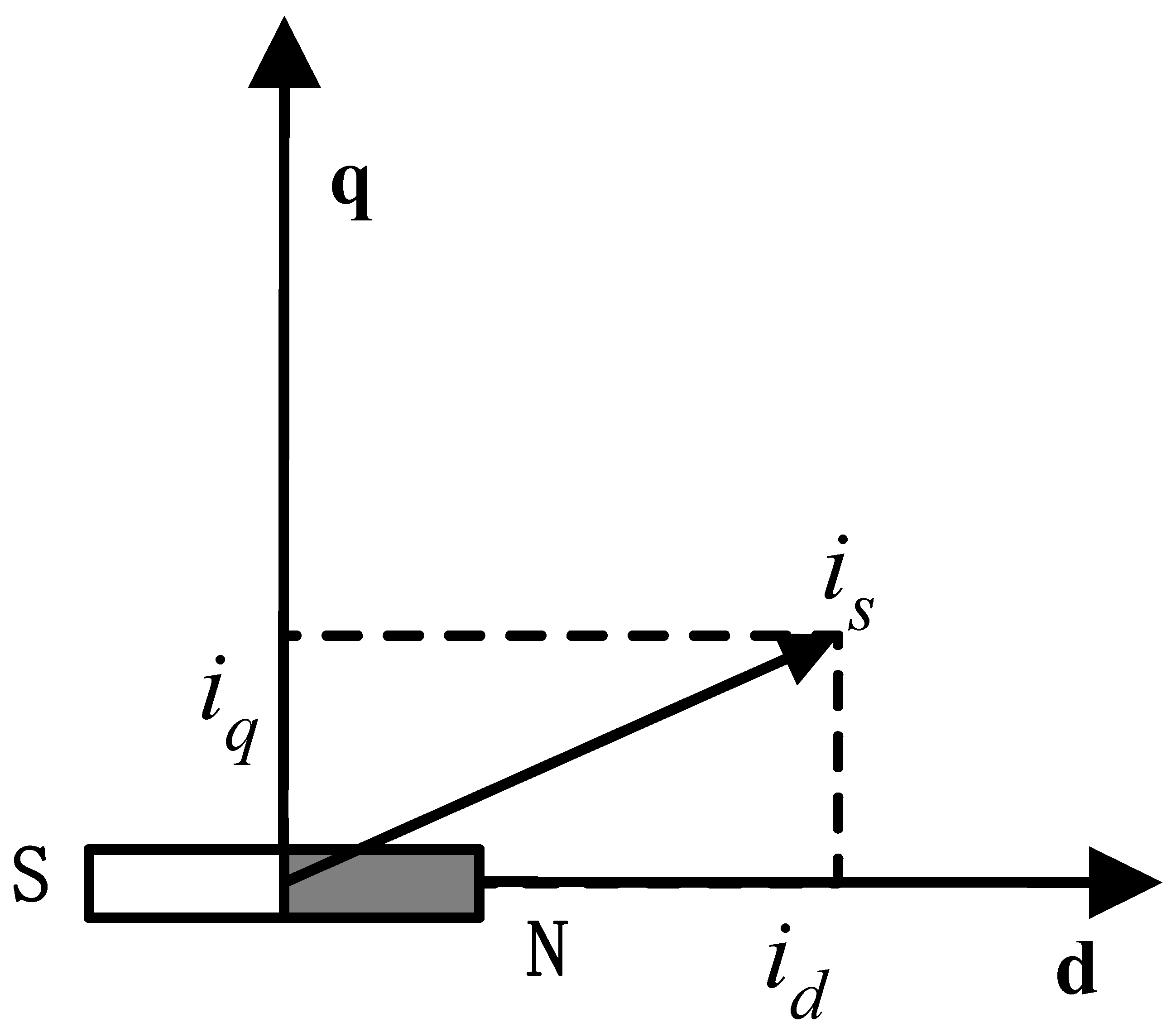
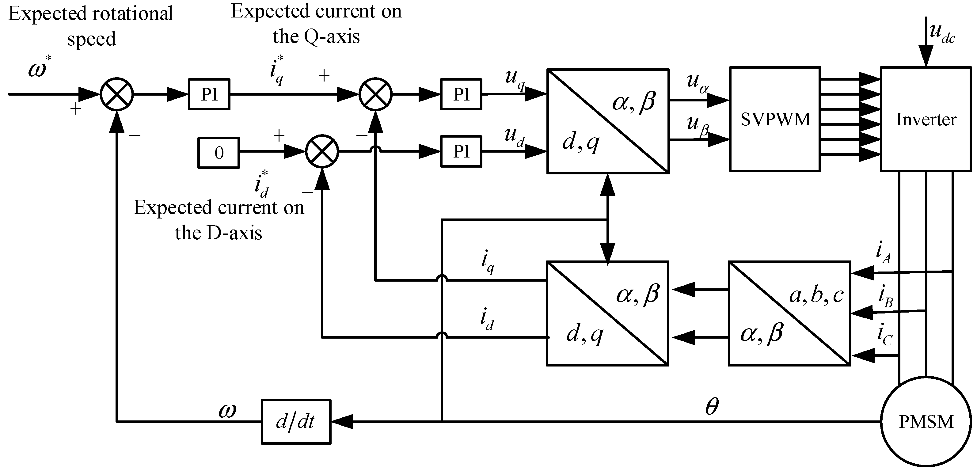
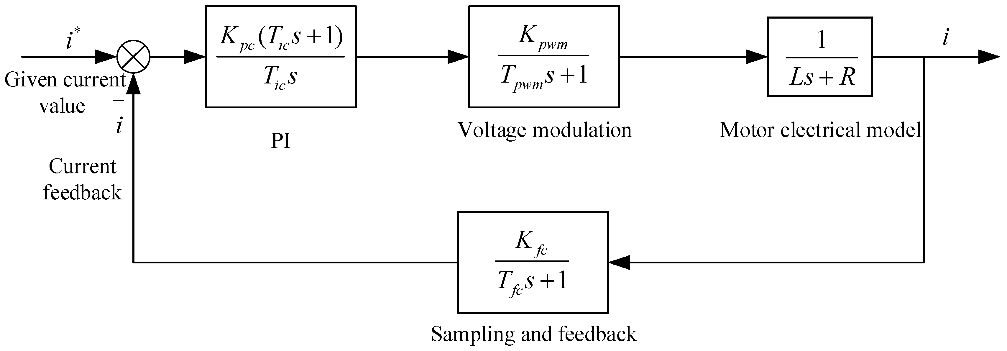
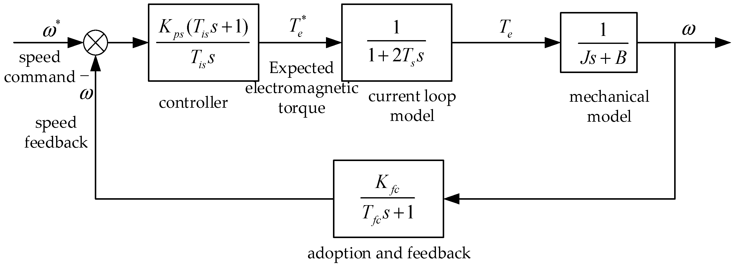
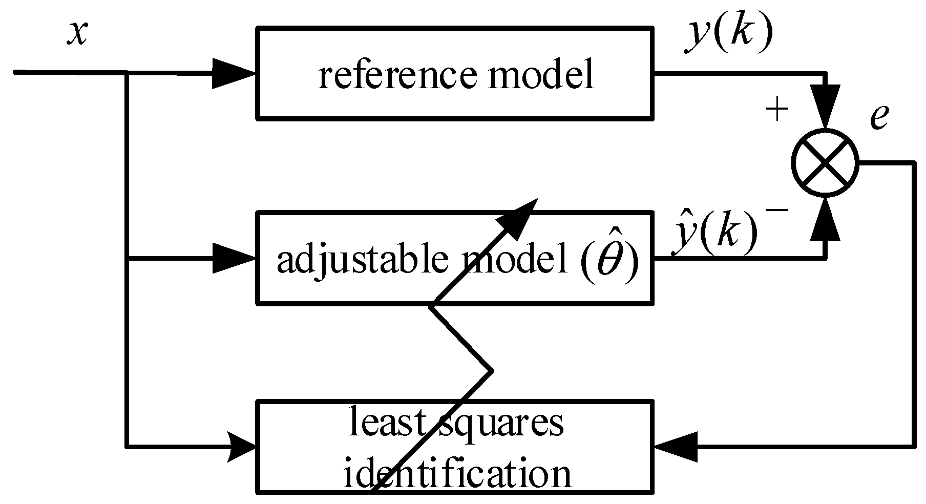
By simply solving for unknown data, the least squares method not only provides a powerful tool but also offers a reliable mathematical means for scientific research and solving practical problems. The schematic diagram of its principle is shown in Figure 8 and Figure 9:

The mathematical expression describing the relationship between the input and output of the least squares model is as follows:

$$y={\theta }_1{x}_1+{\theta }_2{x}_2+\cdots +{\theta }_n{x}_n$$

(33)

In the equation, $\theta$ denotes the object to be estimated, y represents the output value, and x stands for the input value.

When a series of values of x and y are obtained at different times $t1,t2,\cdots ,tn$, the relationship between these data can be expressed using the function of $y(k),x(k)$, thereby deriving the following formula:

$$y(k)={\theta }_1(k)x_1(k)+{\theta }_2(k)x_2(k)+\cdots +{\theta }_n(k)x_n(k)\hspace{1em}k=1,2,\cdots ,m$$

(34)

Rewrite Equation (21) into its matrix form, which is shown as follows:

$$y=X\theta$$

(35)

where

$$\left[\begin{array}{c}y(1)\\ ⋮\\ y(n)\end{array}\right]=\left[\begin{array}{ccc}{x}_1(1)& \cdots & x_n(1)\\ ⋮& & ⋮\\ x_1(m)& \cdots & x_n(m)\end{array}\right]\left[\begin{array}{c}{\theta }_1(1)\\ ⋮\\ {\theta }_n(n)\end{array}\right]$$

(36)

A solution to this equation exists only when the rank of matrix X is n. Moreover, when n = m, the equation has a unique solution. Let $\widehat{\theta }$ be the estimated value; substituting it into Equation (22) yields:

$$y=X\widehat{\theta }$$

(37)

where the estimated value cannot perfectly fit the true value, so the measurement residual vector is defined as:

$$e={(e_1,e_2,\cdots ,e_m)}^T$$

(38)

Its value is:

$$e=y-X\widehat{\theta }$$

(39)

Since residuals can be both positive and negative, making them unsuitable as a direct evaluation criterion, the squared residual is chosen as the evaluation criterion, resulting in:

$$h={\displaystyle \sum _{k=1}^m{e}_k^2=e^{T}e}$$

(40)

Substituting Equation (26) into Equation (27) and taking the derivative yields:

$$h={(y-X\widehat{\theta })}^T(y-X\widehat{\theta })$$

(41)

$${\left.{\displaystyle \frac{\partial h}{\partial \theta }}\right|}_{\theta =\widehat{\theta }}=-2X^{T}y+2X^{T}X\widehat{\theta }=0$$

(42)

Solving Equation (29) gives the corresponding $\widehat{\theta }$ that minimizes the residual. Its value is:

$$\widehat{\theta }={(X^{T}X)}^{-1}{X}^{T}y$$

(43)

The solution to the least squares method is derived by minimizing the sum of squared residuals. A key characteristic of this estimation algorithm is that its implementation process first requires the collection of input and output data, followed by data processing based on the collected data. This process is performed offline, as the entire estimation—from data collection to processing—is completed within a single execution of the algorithm.

3.2.2. Principle of the Recursive Least Squares Method

The least squares method performs excellently in static and offline data processing, but it exhibits significant limitations when dealing with dynamic data sources. Each time new data is input, it is required to reconstruct a matrix for recalculation—this not only consumes substantial controller resources and memory but also creates difficulties for the application of the least squares method.

To overcome this challenge, the Recursive Least Squares (RLS) method is introduced. When new data is acquired, RLS uses this new data along with previously computed results to perform calculations, enabling online updates of parameters. The introduction of this method effectively addresses the problems of the least squares method in dynamic data processing and enhances its adaptability and real-time performance. Its expressions are as follows:

$$\widehat{\theta }(k)=\widehat{\theta }(k-1)+\Delta (k)$$

(44)

where $\Delta (k)$ is the correction term. The core of the RLS method is to calculate the current parameter estimate $\widehat{\theta }(k-1)$ using the previous estimate $\widehat{\theta }(k)$. Based on Equation (30), the parameter estimate $\widehat{\theta }(k)$ at time k is given by:

$$\widehat{\theta }(k)={(X_k^T{X}_k)}^{-1}{X}_k^T{Y}_k$$

(45)

In the equation $X_k=\left[\begin{array}{l}{X}_{k-1}\\ {\phi }^T(k)\end{array}\right]$, ${\phi }^T(k)$ is the input vector at time k, and $Y_k=\left[\begin{array}{l}{Y}_{k-1}\\ y^T(k)\end{array}\right]$ is the output vector at time k.

The matrix inversion lemma is expressed as follows:

$${(A+BCD)}^{-1}=A^{-1}-A^{-1}B{(C^{-1}+D{A}^{-1}B)}^{-1}D{A}^{-1}$$

(46)

Define the covariance matrix P(k) using the matrix inversion lemma, we can derive:

$$\begin{array}{cc}\hfill P(k)& ={\left[P{(k-1)}^{-1}+\phi (k){\phi }^T(k)\right]}^{-1}\hfill \\ & =P(k-1)-P(k-1)\phi (k){\left[1+{\phi }^T(k)P(k-1)\phi (k)\right]}^{-1}{\phi }^T(k)P(k-1)\end{array}$$

(47)

Substituting P(k) into Equation (32) yields:

$$\begin{array}{cc}\hfill \widehat{\theta }(k)& =P(k)[X_{k-1}^T{Y}_{k-1}+\phi (k)y(k)]\hfill \\ \hfill & =\widehat{\theta }(k-1)+{\displaystyle \frac{P(k-1)\phi (k)}{[1+{\phi }^T(k)P(k-1)\phi (k)]}}[y(k)-{\phi }^T(k)\widehat{\theta }(k-1)]\hfill \end{array}$$

(48)

Define the gain matrix K(k), whose value is:

$$K(k)={\displaystyle \frac{P(k-1)\phi (k)}{[1+{\phi }^T(k)P(k-1)\phi (k)]}}$$

(49)

Through the above derivation, the formulas for the recursive least squares method are:

$$\left\{\begin{array}{l}\widehat{\theta }(k)=\widehat{\theta }(k-1)+K(k)[y(k)-{\phi }^T(k)\widehat{\theta }(k-1)]\\ K(k)={\displaystyle \frac{P(k-1)\phi (k)}{[1+{\phi }^T(k)P(k-1)\phi (k)]}}\\ P(k)=[I-K(k){\phi }^T(k)]P(k-1)\end{array}\right.$$

(50)

In the equations, when determining the initial values, we generally set $P(0)=\alpha I$, $\theta (0)=\epsilon$.

3.2.3. Principle of the FFRLS

When changes in the system input or output exceed the adaptive range of the algorithm, the problem of cumulative errors arises, leading to the phenomenon of data saturation—which in turn results in inaccurate estimated parameters or algorithm failure.

Assume there exists a natural number a, b, such that the following equation holds:

$$aI\le {\displaystyle \sum _{k=1}^k\phi (k)}{\phi }^T(k)\le bI$$

(51)

From Equation (38), we can derive:

$$akI+{\displaystyle \frac{I}{P(0)}}\le P^{-1}(k)\le bkI+{\displaystyle \frac{I}{P(0)}}$$

(52)

Taking the reciprocal of both sides of the above equation gives:

$${\displaystyle \frac{I}{ak+\frac{I}{P(0)}}}\le P(0)\le {\displaystyle \frac{I}{bk+\frac{I}{P(0)}}}$$

(53)

From Equation (53), it can be derived that as k approaches infinity, the covariance matrix P(k) also approaches 0. The effect of new input data on updating the identification value gradually diminishes, weakening the correction effect on the result; over time, the update rate of the identification value slows down progressively.

The parameter identification algorithm is considered to have temporal data symmetry. If its evaluation function is the weight assigned to the measurement data, such that the influence of any data point k at time L on the parameter estimation value θ is only a function of the time difference (L − k), rather than the absolute time. When the weight of historical data is too large or the weight of new data is overly emphasized, this symmetry is disrupted.

The traditional recursive least squares method uses fixed-step data, and its evaluation function is $J_{\lambda }={\displaystyle \sum _{k=1}^L[y(k)-{\phi }^T(k)\theta (k){]}^2}$. This seemingly assigns equal weights to all data, but in time-varying systems, it leads to “data saturation”, that is, new data is overwhelmed by historical data, causing the algorithm to lose its update capability and disrupting the dynamic symmetrical matching between the algorithm’s estimated values and the true parameter state of the system.

To address the above issue and overcome the disadvantage of data saturation, the least squares method is optimized by introducing a forgetting factor $\lambda$ to “forget” historical data. Additionally, an evaluation function is defined as follows:

$$J_{\lambda }={\displaystyle \sum _{k=1}^L{\lambda }^{L-k}[y(k)-{\phi }^T(k)\theta (k){]}^2}$$

(54)

In the equation, the value of $\lambda$ generally ranges from 0 to 1. Weight $\omega (k)={\lambda }^{L-k}$ is an exponential function of the time difference (L − k). This function describes a scaling of temporal symmetry, and its time constant is determined by the forgetting factor $\lambda$. By adjusting $\lambda$, a dynamic balance of the weights for new and old data can be achieved, enabling the algorithm logic to form a symmetrical match with the changing patterns of the motor’s operating state.

Equation (41) indicates that the weighting coefficients of the collected data information are related to the change in time. These weighting coefficients are ordered in chronological sequence: the weight of the most recently acquired data information is 1,

Based on the above derivation process of the recursive least squares algorithm, the parameter identification formulas for the recursive least squares algorithm with a forgetting factor (FF-RLS) can be derived as follows:

$$\left\{\begin{array}{l}\widehat{\theta }(k)=\widehat{\theta }(k-1)+K(k)[y(k)-{\phi }^T(k)\widehat{\theta }(k-1)]\\ K(k)={\displaystyle \frac{P(k-1)\phi (k)}{[\lambda +{\phi }^T(k)P(k-1)\phi (k)]}}\\ P(k)={\displaystyle \frac{1}{\lambda }}[I-K(k){\phi }^T(k)]P(k-1)\end{array}\right.$$

(55)

In the equation, regarding the method for determining the initial values $P(0)$ and $\widehat{\theta }(0)$, generally, $P(0)=\alpha I$ and $\theta (0)=\epsilon$ are adopted. For the forgetting factor $\lambda$, its value is generally not less than 0.9; for linear relationship identification, the forgetting factor is usually selected within the range of 0.9 to 1. When the forgetting factor $\lambda$ = 1, the FFRLS is equivalent to the ordinary recursive least squares method.

3.2.4. Simulation Analysis

The mechanical equation of a PMSM is as follows:

$$T_e=J{\displaystyle \frac{d{\omega }_m}{dt}}+B{\omega }_m+T_L$$

(56)

In the equation, $T_e$ denotes the electromagnetic torque, J denotes the moment of inertia of the servo system, B denotes the viscous friction coefficient, ${\omega }_m$ denotes the rotor mechanical angular velocity, and $T_L$ denotes the load torque.

To discretize the above equation, the derivative term is replaced by the backward difference method.

At time step k:

$$T_e[k-1]=J{\displaystyle \frac{\omega [k]-\omega [k-1]}{T_s}}+B\omega [k-1]+T_L[k-1]$$

(57)

At time step k + 1:

$$T_e[k]=J{\displaystyle \frac{\omega [k+1]-\omega [k]}{T_s}}+B\omega [k]+T_L[k]$$

(58)

where $T_s$ is the sampling period. Considering that within a short sampling interval, the load torque remains unchanged $T_L[k]-T_L[k-1]=0$, it can thus be neglected. Meanwhile, the viscous friction coefficient B has a small value; within a short time interval, the product of the velocity change and the viscous friction coefficient can be regarded as a small quantity $B\omega [k]-B\omega [k-1]=0$ and thus can also be neglected.

Subtracting Equation (44) from Equation (45) yields:

$$T_e[k]-T_e[k-1]=J{\displaystyle \frac{\omega [k+1]-2\omega [k]+\omega [k-1]}{T_s}}$$

(59)

Rewriting the above equation into the standard form of the least squares method gives:

$$\omega [k+1]-2\omega [k]+\omega [k-1]={\displaystyle \frac{T_s}{J}}(T_e[k]-T_e[k-1])$$

(60)

To simplify the calculation, based on the above equation, we obtain:

$$\left\{\begin{array}{l}\widehat{\theta }=T_s/J\\ \phi (k)=\Delta T_e(k)=T_e(k)-T_e(k-1)\\ y(k)=\Delta \omega (k+1)-\Delta \omega (k)\end{array}\right.$$

(61)

Substituting Equation (48) into Equation (42) yields:

$$\left\{\begin{array}{l}{\displaystyle \frac{T_s}{\widehat{J}}}(k)={\displaystyle \frac{T_s}{\widehat{J}}}(k-1)+K(k)[\Delta \omega (k+1)-\Delta \omega (k)-\Delta T_e(k){\displaystyle \frac{T_s}{\widehat{J}}}(k-1)]\\ K(k)={\displaystyle \frac{P(k-1)\Delta T_e(k)}{\lambda +\Delta T_e^2(k)P(k-1)}}\\ P(k)={\displaystyle \frac{1}{\lambda }}[1-K(k)\Delta T_e(k)]P(k-1)\end{array}\right.$$

(62)

According to Equation (62), a MATLAB/Simulink model is constructed, and its parameters are shown in

Table 1. PMSM Parameter table.

Parameter	Quantitative Value
power/W	750
Stator Winding Resistance/Ω	1.2
d-axis Inductance/H	0.0043
q-axis Inductance/H	0.0043
inertia/kg·m2	0.0004
Viscous Friction Coefficient/N.m.s	0.001
Flux Linkage/Wb	0.097
Number of Pole Pairs/n	4

.

In this simulation, the core formula is $J={\displaystyle \frac{\Delta T_e[k]}{\raisebox{1ex}{$\Delta \omega [k+1]-\Delta \omega [k]$}\!\left/ \!\raisebox{-1ex}{$T_s$}\right.}}$. If the speed variation $\Delta \omega$ is zero, the denominator of the formula approaches zero, which easily leads to abnormal identification values; if the torque variation $\Delta T_e$ is zero, the numerator becomes zero, resulting in incorrect results. Moreover, the identification accuracy is strongly correlated with the input excitation. To address this, the input speed in the simulation is set as a triangular wave with an amplitude of 60 rad/s and a period of 0.12 s. Its linear variation characteristic can stably provide non-zero speed change rates and torque variations, avoiding issues such as sinusoidal wave identification interruption and square wave current impact. The selection of parameters balances the motor’s rated operating conditions and data acquisition efficiency.

In the algorithm update process, it is necessary to first determine whether the speed and torque variations are greater than the threshold. If the condition is satisfied, the algorithm is updated; otherwise, it remains unchanged. This step is designed to filter out the Gaussian white noise of the sensor. The threshold needs dynamic adjustment: a baseline value is initially set according to the noise level, then optimized based on the simulation results, and adapted to different operating conditions. This lays a foundation for the reliable operation of the subsequent FFRLS. The speed feedback waveform, feedback torque waveform, $\Delta \omega$ waveform, and $\Delta T_e$ waveform are shown in Figure 10.

Among them, the absolute value processing is performed on the torque variation and the moment variation. It can be seen from the above figure that the torque variation thresholds are set as $\Delta T_e>0.12 \mathrm{N}·\mathrm{m}$ $\Delta \omega >1.25 \mathrm{rad}/\mathrm{s}$. Since the actual friction model has large mutations at low speeds, the moment of inertia identification is not performed under low-speed conditions either.

When using the FFRLS algorithm to identify the moment of inertia of the servo system, since the input values of the identification algorithm are the speed variation and the current variation, it is necessary to select an appropriate calculation period. After determining the calculation period, an appropriate forgetting factor should be determined through experimental debugging. For the current laboratory servo motor platform, the interrupt calculation period is designed as 10 kHz in the controller. In this simulation, the time period used for parameter identification should be larger than the interrupt calculation period, so it is set to 1 ms.

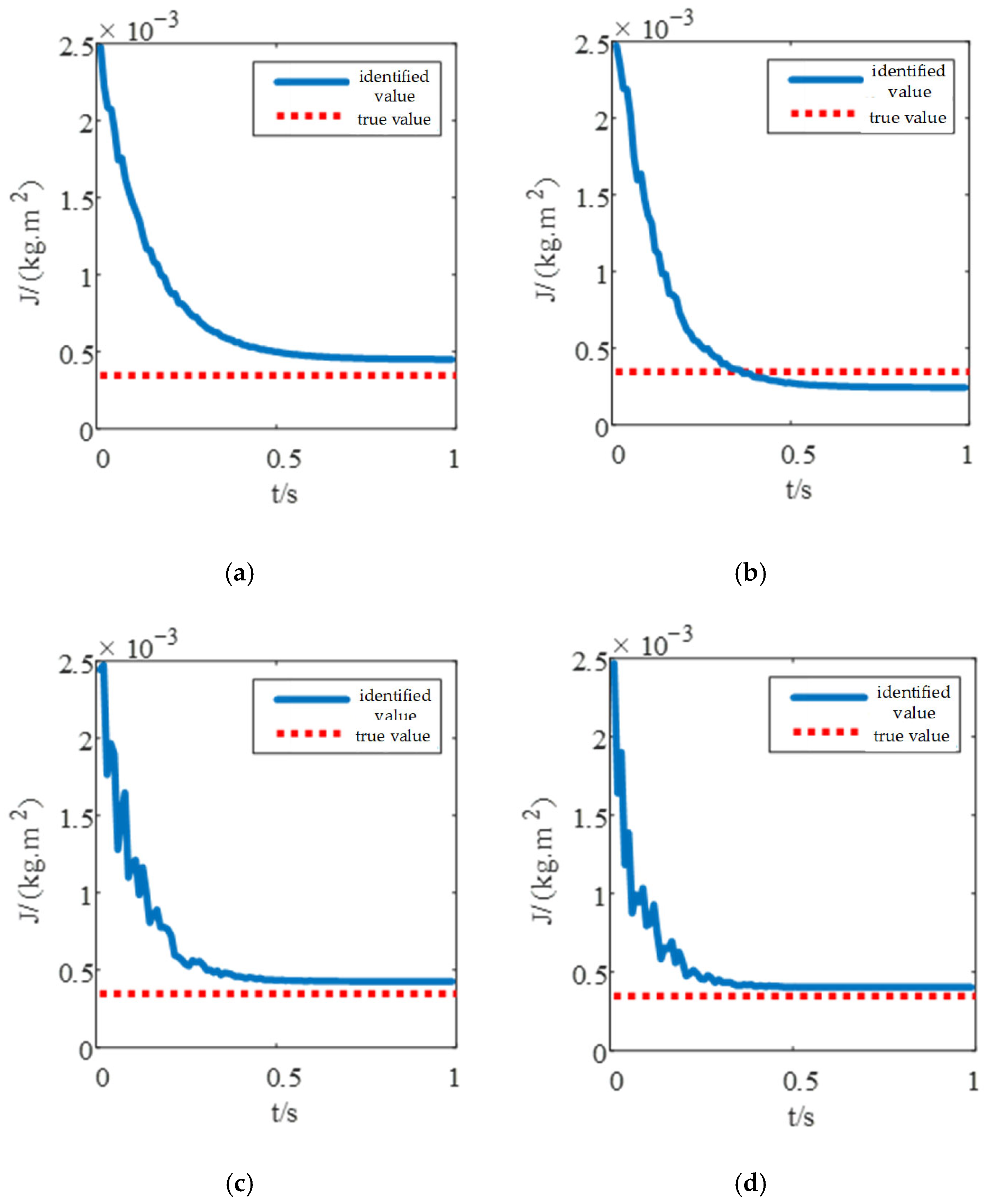
When selecting the forgetting factor, a small value is usually not chosen. In this simulation, the method of controlling variables is adopted, and the forgetting factor is set to 0.98, 0.96, 0.94, and 0.92, respectively, to perform online identification of the moment of inertia of the servo system. The identification results are shown in Figure 11.

It can be seen from Figure 11 that the selected value of the forgetting factor $\lambda$ is closely related to the convergence time, oscillation amplitude, and accuracy. Specifically, the smaller the value of $\lambda$, the faster the convergence speed and the higher the accuracy; however, there is also a risk of oscillation in the convergence curve. In contrast, the larger the value of $\lambda$, the smoother the convergence curve, but its convergence speed and identification accuracy are unsatisfactory. Therefore, for this simulation, selecting the forgetting factor $\lambda$ = 0.92 is quite appropriate. The convergence time and corresponding accuracy for different forgetting factors are shown in

Table 2. The convergence time and corresponding accuracy for different forgetting factors.

The Value of $\mathit{\lambda }$	Convergence Time/s	Identified Value/(kg·m2)	Actual Value/(kg·m2)	Identification Accuracy/%
0.98	0.62	$4.7\times {10}^{-4}$	$4.0\times {10}^{-4}$	+17.5
0.96	0.55	$3.6\times {10}^{-4}$	$4.0\times {10}^{-4}$	−10
0.94	0.47	$4.3\times {10}^{-4}$	$4.0\times {10}^{-4}$	+7.5
0.92	0.39	$4.2\times {10}^{-4}$	$4.0\times {10}^{-4}$	+5

:

Analysis of Table 2 reveals the following: When $\lambda$ = 0.98, the identification accuracy is +17.5%, which is relatively poor and cannot be applied to the control of the speed loop. When $\lambda$ = 0.92, the identification accuracy is +5%, representing a 12.5% improvement compared to when $\lambda$ = 0.98; the convergence time is 0.39 s, which is 0.23 s shorter than that when $\lambda$ = 0.98. Therefore, different identification effects are produced when different forgetting factors are selected.

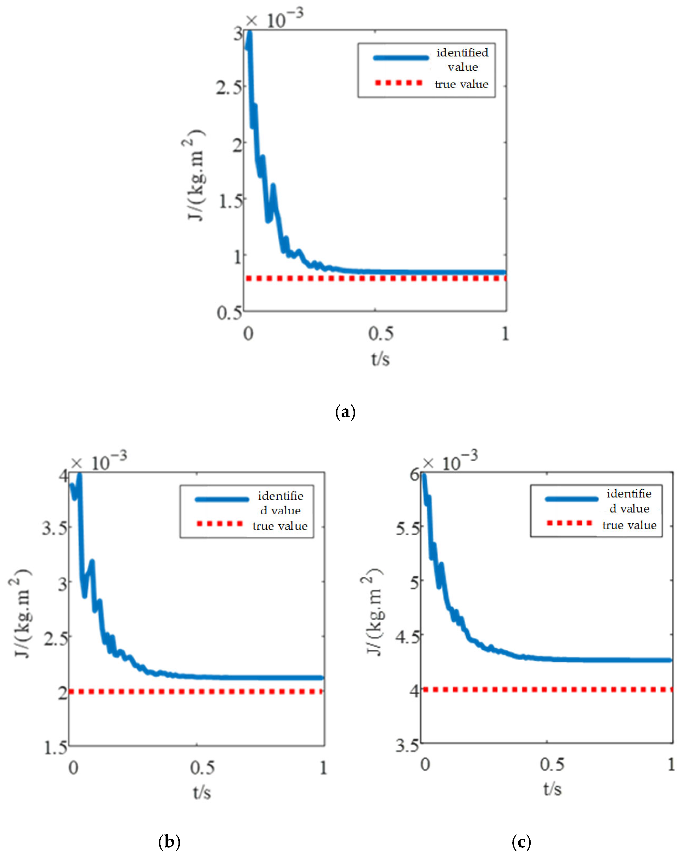
In many practical applications, the operating scenarios of PMSM are far from being limited to bearing the moment of inertia of the no-load motor itself. Generally speaking, such system application scenarios may involve multiple power levels, and the motor may need to operate under various load conditions. These loads can vary according to task requirements and may be dynamically changing. Therefore, for such systems, the accurate identification of multiple times the moment of inertia has become a basic and critical requirement. Furthermore, identifications are performed twice, five times, and ten times the moment of inertia, respectively, and the identification results are shown in Figure 12:

It can be seen from Figure 12 that under the condition of twice the inertia, the identification speed is the fastest and the identification accuracy is also the highest. When gradually increasing to ten times the inertia, the identification speed and accuracy decrease relatively, but the identification curve is smoother. This is because the response speed of the speed loop decreases under high load conditions. The convergence time and corresponding accuracy for different inertia values are shown in

Table 3. The convergence speed and accuracy of inertia identification.

Inertia Multiple	Convergence Time/s	Identified Inertia/(kg·m2)	Actual Inertia/(kg·m2)	Identification Accuracy/%
Double inertia	0.40	$8.5\times {10}^{-4}$	$8.0\times {10}^{-4}$	+6.3%
Fivefold inertia	0.42	$2.14\times {10}^{-3}$	$2.0\times {10}^{-3}$	+7.2%
Tenfold inertia	0.47	$4.32\times {10}^{-3}$	$4.0\times {10}^{-3}$	+7.9%

:

Analysis of Table 3 reveals that as the load inertia increases, the identification accuracy decreases while the identification convergence time increases. This highlights the importance of accurately identifying the load’s moment of inertia under high-multiple load conditions. Accurate inertia identification is not only crucial for improving system control precision but also a necessary prerequisite for ensuring dynamic response and stable system operation.

By employing the recursive least squares method with a forgetting factor for online identification of the moment of inertia, an effective symmetric relationship of dynamic approximation between the identified value and the true value is achieved. This method continuously revises the identification results based on real-time operating data, enabling the estimated moment of inertia to adaptively symmetrically track changes in the true inertia. Consequently, high parameter symmetry is maintained under time-varying operating conditions. The realization of this symmetry not only significantly enhances identification accuracy and the adaptability of system control but also lays a critical foundation for high-precision servo control and stability assurance.

3.2.5. Experimental Verification and Analysis

For the identification of moment of inertia using FFRLS, the following steps are implemented: first, delay correction is performed on the q-axis current signal and rotational speed signal collected by the AD converter to ensure synchronization between the identification program and data acquisition; then, the input signals are judged to screen out valid data that meets the identification conditions; subsequently, least squares fitting is conducted on the valid data; finally, the identified moment of inertia value is output through iterative loop calculations.

This experiment is built on a servo motor controller based on the STM32F446 processor, and the corresponding algorithm development has been completed. The experimental control platform is shown in Figure 13a, which mainly consists of a host computer, a circuit board, an oscilloscope, and a DC power supply. The experimental motor setup is shown in Figure 13b, which mainly includes an experimental motor, a load motor, and inertia disks. By replacing different inertia disks, experimental conditions with multiple times the base inertia can be created.

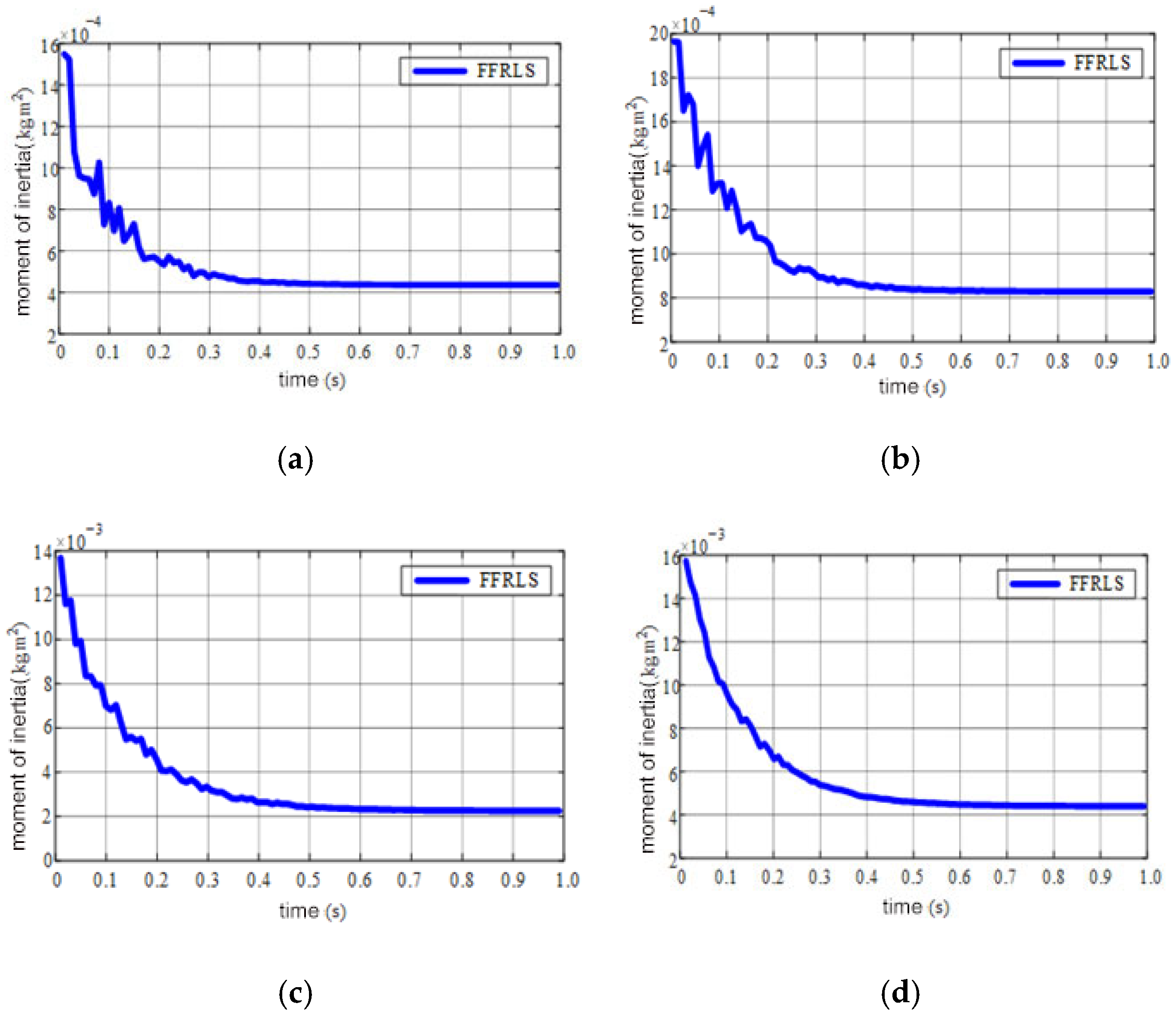
Since the input values of the FFRLS algorithm for identifying the moment of inertia are the speed variation and current variation, the convergence speed and identification accuracy of the algorithm are strongly related to the intensity of the speed excitation. Therefore, in this experiment, the speed reference is set as a triangular wave, and the forgetting factor FFRLS is used to identify the moment of inertia. Experiments under no-load conditions, double load inertia, fivefold load inertia, and tenfold load inertia are conducted, respectively, and the experimental results are shown in Figure 14.

Based on the above experimental results, in order to intuitively present the identification accuracy and convergence time of the identification algorithm, the identification results under different inertia conditions are shown in

Table 4. Experimental results.

Inertia Multiple	Convergence Time/s	Identified Inertia/(kg·m2)	Actual Inertia/(kg·m2)	Identification Accuracy/%
No-load inertia	0.41	$4.21\times {10}^{-4}$	$4.0\times {10}^{-4}$	+5.2%
Double inertia	0.45	$8.5\times {10}^{-4}$	$8.0\times {10}^{-4}$	+5.6%
Fivefold inertia	0.51	$2.14\times {10}^{-3}$	$2.0\times {10}^{-3}$	+6.3%
Tenfold inertia	0.59	$4.32\times {10}^{-3}$	$4.0\times {10}^{-3}$	+7.9%

.

As shown in Table 4, under the no-load condition, the identification accuracy is 5.2% and the convergence time is 0.41 s; under the tenfold inertia condition, the identification accuracy is 7.9% and the convergence time is 0.59 s. These results indicate that the algorithm can quickly and accurately capture the actual inertia of the system when there is no load disturbance, further verifying the rationality of the earlier simulation model and the adaptability to the actual system.

In conclusion, the FFRLS algorithm proposed in this paper meets the requirements of practical engineering applications in terms of both identification accuracy and convergence time for moment of inertia identification. It is conducive to quickly obtaining accurate system parameter estimation in real-time or rapidly dynamically changing system environments, thereby helping to improve the flexibility and reliability of the overall system control strategy.

4. Conclusions

4.1. Conclusions and Summary of the Work

Aiming at the core problem in the vector control of PMSM servo systems—namely, the asymmetric imbalance between the “given-feedback” speeds caused by the lack of online identification of the moment of inertia—this work constructs a moment of inertia identification system that balances accuracy and dynamics through mathematical modeling, algorithm optimization, and parameter analysis. The main research work and achievements are as follows:

1. Establishment of a dual-closed-loop control mathematical model and completion of PI parameter tuning

A mathematical model of the PMSM current-speed dual closed-loop vector control system was established, clarifying the hierarchical control relationship of the dual loops and the parameter coupling characteristics. To meet the dual symmetric tracking requirements of the current loop and the speed loop, the theoretical tuning of PI controller parameters was completed. The influences of electrical parameters and mechanical parameters on the dynamic characteristics of the loops were analyzed. Among these, changes in the moment of inertia directly lead to tracking lag or overshoot in the speed loop, destroying the symmetric matching between “given and feedback”, which provides a core basis for the subsequent optimization of the identification algorithm.

2. Analysis of the limitations of the traditional Least Squares method

The traditional LS method has significant shortcomings: its static mechanism of “equal weight for all data” leads to asymmetric imbalance between “data weight and working condition characteristics”. Under steady-state working conditions, noise in historical data dilutes effective information; under dynamic working conditions, real-time information contained in new data cannot be prioritized for response. In addition, the batch data processing mode is prone to data saturation, making the identification results lose the ability to achieve dynamic symmetric matching with the “actual inertia”. Meanwhile, this method has weak anti-interference ability and high requirements for excitation signals, making it difficult to meet the needs of engineering application scenarios.

3. Proposition of the Forgetting Factor Recursive Least Squares method and verification of its effectiveness

To address the shortcomings of traditional algorithms, the FFRLS method was proposed: by introducing a forgetting factor $\lambda$, a dual symmetric adaptive mechanism for “working condition changes and noise suppression” was constructed. Adjusting $\lambda$ can balance “historical data” and “real-time dynamic data “, realizing accurate symmetric matching between “algorithm logic and motor state”. The recursive structure avoids data saturation, enabling the identification results to continuously track the “actual inertia” and maintain the symmetric relationship between them. Simulation and experimental results show that when $\lambda$ = 0.92, the identification accuracy reaches +5% with a convergence time of only 0.39 s; even under working conditions of 2×, 5×, and 10× inertia, dynamic symmetry can still be maintained. Moreover, on embedded platforms, it can efficiently achieve the symmetric balance of “accuracy, speed, and robustness” and reduce the requirements for excitation signals.

4.2. Work Outlook

This work focuses on the algorithm optimization of PMSM moment of inertia identification. However, limited by time and existing research conditions, there is still room for optimization and expansion. Future in-depth exploration can be carried out in the following directions:

1. Improvement of signal delay correction and noise suppression

Currently, only the speed signal has been subjected to delay correction. Due to the shorter current sampling period than the parameter identification period, no delay correction has been implemented for the current signal. In subsequent research, consideration can be given to applying delay correction to the current signal as well, while exploring the combination of filtering algorithms to suppress sampling noise. This will further eliminate the asymmetric deviation between “measured values and true values” and improve identification accuracy.

2. Expansion of multi-parameter identification capabilities

The existing FFRLS method can only realize single-parameter identification of the moment of inertia and cannot simultaneously identify the load torque and viscous friction coefficient. The current method of eliminating these two parameters through difference calculation indirectly reduces the accuracy of inertia identification. In the future, attempts can be made to use intelligent algorithms such as Radial Basis Function Neural Network to construct a multi-parameter synchronous identification model, which can simultaneously obtain the moment of inertia, load torque, and viscous friction coefficient. This will solve the problem of “single-parameter identification ignoring interference from other parameters” and further improve the integrity and accuracy of system control.