Article

A Robust Lagrangian Implicit Material Point Method for Accurate Large-Deformation Analysis

1
Institute of Applied Mechanics, Ningbo Polytechnic University, Ningbo 315800, China
2
Institute of Geotechnical Engineering, Ningbo University, Ningbo 315211, China
*
Author to whom correspondence should be addressed.
Symmetry 2025, 17(11), 1876; https://doi.org/10.3390/sym17111876
Submission received: 21 September 2025 / Revised: 21 October 2025 / Accepted: 25 October 2025 / Published: 5 November 2025
(This article belongs to the Special Issue Feature Papers in Section "Engineering and Materials" 2025)

Abstract

The material point method (MPM) has shown significant potential for simulating problems involving large deformations. However, many implicit MPM formulations based on the traditional Updated Lagrangian (UL) scheme still face challenges in terms of computational stability. In this study, we propose a novel Lagrangian equilibrium formulation for an implicit MPM that is tailored to large-deformation problems. (1) The previously converged state is utilized to simplify stiffness matrix computations, thereby improving the stability of the algorithm. (2) The framework supports a variety of high-order interpolation functions, which effectively mitigate numerical artifacts such as cell-crossing errors. (3) The B-bar technique is further incorporated to suppress spurious stress oscillations in the incompressible limit. The proposed method is validated through two classical benchmark tests, the simple shear of a single element and the cantilever beam problem, by comparing the simulation results with analytical solutions and alternative numerical approaches. Finally, its capability is demonstrated in slope stability and strip footing analyses, confirming the superior accuracy, stability, and robustness of the method for large-deformation elastoplastic problems.

1. Introduction

Numerical methods based on the Lagrangian method have always been applied to calculate solid problems, and the finite element method (FEM), as a kind of mesh-based approach, has attracted much attention due to its power and accuracy in practical applications. However, the FEM is likely to suffer from mesh distortion in large-deformation problems. In order to overcome and eliminate the limitations due to meshes, various mesh-free/meshless methods have been proposed, such as smoothed particle hydrodynamics (SPH) [1], the element-free Galerkin method (EFGM) [2], the particle finite element method (PFEM) [3], the arbitrary Lagrangian–Eulerian method (ALE) [4], and the MPM.
The MPM was developed by Sulsky et al. [5] to simulate solid dynamics problems. It is an extension of the particle-in-cell (PIC) [6] and fluid-implicit-particle (FLIP) [7] methods. The MPM is a coupled Euler–Lagrange method which combines the advantages of both the Eulerian and Lagrangian methods. The key idea behind the MPM is that the information about a deformed body (i.e., displacement, velocity, acceleration, strain, and stress) is saved on the material points. The information is mapped by an interpolation function to the nodes of a background mesh on which the equations of motion are solved in every loading step. The new state can be obtained and is remapped to the material point for updating the state of material points. The MPM attempts to avoid the numerical difficulties arising from nonlinear convective terms associated with Eulerian problem formulation, while at the same time preventing grid distortion, typically encountered within mesh-based Lagrangian formulations.
Classically, the MPM uses linear interpolation functions. However, the gradients of these interpolation functions are discontinuous at element boundaries. This leads to the so-called cell-crossing errors [8] when material points cross this discontinuity. Cell-crossing errors can significantly influence the quality of a numerical solution and may eventually lead to a lack of convergence [9]. In order to mitigate the cell-crossing error, the linear interpolation functions are replaced by higher-order interpolation functions, including the Generalized Interpolation Material Point (GIMP) [8], Convected Particle Domain Interpolation (CPDI) [10], the Dual Domain Material Point (DDMP) [11], the B-spline material point method (BSMPM) [12], and the Moving Least Squares (MLS) method [13]. However, when using higher-order interpolation functions, the mapping range of the material points may extend beyond the grid they belong. In explicit algorithms, the information from the material points is mapped onto the grid nodes, and the solution of the balance equation is obtained by performing vector operations directly on the nodes. Therefore, the expansion of the material point influence range does not cause any issues. However, in implicit algorithms, the balance equation is solved by assembling a stiffness matrix. If the stiffness matrix is assembled based on elements, as in the finite element method, this can lead to problems of overlapping or missing physical information. To avoid such issues, in implicit material point methods, the stiffness matrix should be assembled based on particles.
In the initial phases of research, many researchers concentrated on employing an explicit approach and on the application of an explicit MPM, for instance, for impact problems [14,15], explosions [16,17], fractures [18], and slope failures [19,20,21]. Nevertheless, there are advantages to adopting an implicit approach, including (1) enhanced stability, (2) improved error control, and (3) increased loading step size. Wang et al. [22] and Yuan et al. [23] developed an implicit MPM framework within a UL formulation based on the small-strain, large-rotation theory. They subsequently performed numerical simulations of geotechnical problems to evaluate their applicability. However, within their UL framework, the second Piola–Kirchhoff stress (PK) was directly equated to the Cauchy stress, and the evolution of the gradient of interpolation functions was not considered at each incremental step. These simplifications result in convergence challenges when analyzing large-deformation problems, such as cantilever beam bending, necessitating the introduction of artificial stiffness to complete the simulations. For further details, refer to Wang et al. [22]. In contrast, Charlton et al. [24] developed an UL implicit MPM framework that is suitable for large-strain theory, wherein the gradient of interpolation functions is updated at each incremental step. Building upon the work of Charlton et al. [23], Coombs et al. [25,26] proposed a novel Lagrangian framework that satisfactory results in simulating cantilever beam bending. However, their approach requires a substantial number of material points per initial grid cell, typically exceeding 36, as detailed in Coombs et al. [24]. Furthermore, the application of large-strain theory necessitates the recalculation and reassembly of a more complex tangent stiffness matrix at each iteration, which significantly increases computational costs. A summary of the features implemented in the current work is presented in Table 1, comparison them to previous implicit MPM developments for large deformation simulation.
The main motivation of this paper is to present a novel Lagrangian formulation of the equilibrium equation within the context of the MPM framework. The paper is organized as follows. Section 2 reviews the applicability of traditional UL formulations for MPM. In Section 3, a novel Lagrangian formulation of equilibrium and the corresponding MPM discretization are introduced, including small strain with large rotations for the constitutive model. Section 4 outlines the quasi-static computational processes for the implicit MPM. In Section 5, the proposed MPM framework is verified and used to investigate the methods’ capacities in various examples. Conclusions are given in Section 6.

2. Traditional UL Formulation

In the traditional UL formulation [22,23], using the last know configuration as a reference, the governing equation can be expressed in the weak form
V t δ ε T S t + Δ t d V = S t δ u T τ t + Δ t d Γ + V t δ u T b t + Δ t d V
where S t + Δ t is the second PK tensor at time t + Δt, δε is the virtual Green-Lagrange strain tensor; δu is the virtual displacement tensor; τ is prescribed part of the traction on the surface Γ ; b is the body load; the Γ and V are, respectively, the part of face on the continuity and the volume of continuity.
Due to the current configuration as a reference configuration, the second PK S t + Δ t at time t + Δt can be decomposed and simplified into the stress σ t at time t and increment stress Δ σ . The details are not provided here, but can be referred to in works [21,22] for more information.
S t + Δ t = S t + Δ σ = σ t + Δ σ
The relation can be expressed between the stress increment and the strain increment:
Δ σ = C Δ ε
where C is the material stress–strain tensor, the strain increment Δε is composed of the linear strain increment Δe and nonlinear strain increment Δη, the strain increment Δε can be written as
Δ ε = Δ e + Δ η
Substituting Equations (2)–(4) into Equation (1), the governing equation can be obtained as
V t δ Δ e T C Δ e d V + V t δ Δ e T C Δ η d V + V t δ Δ η T C Δ e d V + V t δ Δ η T C Δ η d V + V t δ Δ η T σ t d V = S t δ u T τ t + Δ t d Γ + V t δ u T b t + Δ t d V V t δ Δ e T σ t d V
where δ e and δ η are the linear and nonlinear strain tensors corresponding to the virtual displacements. In order to facilitate the account, the second, third, and fourth terms on the left-hand side are neglected in Equation (5). Thus, the governing equation is rewritten as:
V t δ Δ e T C Δ e d V + V t δ Δ η T σ t d V = S t δ u T τ t + Δ t d Γ + V t δ u T b t + Δ t d V V t δ Δ e T σ t d V
For reducing the effect of a rigid body rotation, the objective stress rate (Jaumann stress rate) is adopted. The relation between the Cauchy stress increment and Jaumann stress increment is written as
Δ σ J = Δ σ + σ t Δ W Δ W σ t = C J Δ e
where CJ is the fourth-order tensor of elastic moduli, W is the non-objective spin tensor, it can be given as
Δ W = 1 2 [ ( u ) ( u ) T ]
where u is the displacement gradient. By substituting Equation (7) into Equation (6), the final equilibrium equation of traditional UL formulation can be rewritten as
V t δ Δ e T C J Δ e d V + V t δ Δ η T σ t d V + V t δ Δ e T ( Δ W σ t σ t Δ W ) d V = Γ t δ u T τ t + Δ t d Γ + V t δ u T b t + Δ t d V V t δ Δ e T σ t d V

Spatial Discretization of Equilibrium Equation for Traditional MPM

The first term of Equation (9) on the left hand in equilibrium can be expressed as
V t δ Δ e T C J Δ e d V = V t B L T C J B L d V Δ u = i = 1 n p B L T C J B L V p Δ u = K mat Δ u
where K mat presents material stiffness matrix, BL is the linear strain–displacement matrix, Vp is the volume of material point, np is the total number of material points in the solid body.
The other terms of Equation (9) on the left hand, which is called as geometric stiffness matrix. The geometric stiffness matrix is given as
V t δ Δ η T σ t d V + V t δ Δ e T ( Δ W σ t σ t Δ W ) d V = V t B N L T σ ¯ B N L d V Δ u = i = 1 n p B N L T σ ¯ B N L V p Δ u = K geo Δ u
where K geo denotes geometric stiffness matrix, BNL is the nonlinear strain–displacement matrix, σ ¯ is the stress matrix. The terms on the right-hand side of Equation (9), which are regarded as external load, are calculated as
f e x t = Γ t δ u T τ t + Δ t d Γ + V t δ u T b t + Δ t d V = i = 1 n p N i p b t + Δ t V p + i = 1 n p N i p τ p h p 1
where fext is the external load on the nodes, Nip is the interpolation function, and hp is the characteristic length of particle. The internal force f i n t   of the equilibrium equation is defined as
f i n t = V t δ Δ e T σ t d V = i = 1 n p B L T σ t V p t
At last, the equilibrium equation in matrix form can then be formulated as
K mat + K geo δ u k = f ext f int
where δuk is the iterative displacement vector, k is the number iterative. For the specific distribution of stiffness matrix and strain–displacement matrix, refer to References [22,23].

3. The Proposed Lagrangian Formulation

Lagrangian mechanics for large deformation problems is primarily categorized into two approaches: the Total Lagrangian (TL) formulation based on the original configuration, and the UL formulation, which is based on the current configuration, similar to the finite element method. Notably, the UL formulation is more suitable for MPM than the TL formulation. In MPM, the background grid is typically reset after each load step, presenting inherent challenges for the application of the TL formulation. A significant issue arises because the strain–displacement matrix depends on the derivatives of the interpolation functions with respect to the original coordinates. Although it is theoretically possible to recover these derivatives through the total deformation gradient, as shown in Figure 1, they would only be applicable to the element in which the material point is currently located. Crucially, there is no guarantee that a material point will remain in the same element throughout the analysis, as the deformation history of the background grid is not retained between load steps. Implementing the TL formulation in the MPM would necessitate not only mapping the interpolation functions back to the original coordinates but also storing the grid deformation throughout the entire analysis process. These added requirements would ultimately undermine the computational efficiency of the MPM.
Figure 1 illustrates the deformation of a material point from the reference configuration to the current configuration during a loading step. As the material point moves from X ¯ p to x p without changes in the local coordinates of its parent element, the deformation gradient increment ΔF accurately captures the variations in the derivatives of the interpolation functions. For specific descriptions, please refer to the work of Charlton et al. [24].

3.1. Equilibrium Equation for Proposed MPM

This section presents a new approach for achieving equilibrium in the MPM, using the previously converged state as the reference configuration. The proposed Lagrangian formulation is defined by the following statement of equilibrium:
d i v P ¯ + ρ b = 0
where ρ   is the mass density, b is the body force, P ¯ is the nominal stress tensor, which is the Cauchy stress pulled back to the previously converged state. It can be obtained as
P ¯ = J σ F T
where F is the deformation gradient tensor and J is the determinant of Jacobian matrix, which is J = det ( F ) . The weak form of the equilibrium equation in an arbitrary region V can be expressed as follows:
V δ u T x P ¯ d V = S δ u T q d Γ + V δ u T ρ b d V
where Γ is the boundary surface, q is subjected to tractions vector. To clearly represent the proposed method, the incremental form of weak formulation is given as
V δ u ˙ x T P ¯ ˙ t + Δ t Δ t d V = Γ δ u ˙ T Δ q d Γ + V δ u ˙ T ρ Δ b d V
where Δt is the time increment, Δq is the increment form of tractions vector, Δb is the increment form of body force vector, P ¯ ˙ t + Δ t is the nominal stress rate at the current time t + Δt.
The nominal stress rate can be transformed into the Cauchy stress rate by using the method proposed in Yatomi et al. [29], that is
P ¯ ˙ t + Δ t = P ¯ t + Δ t P ¯ t / Δ t = σ ˙ + t r D σ t σ t L T
where σ ˙ is the Cauchy stress rate tensor, σ t is the Cauchy stress tensor at time t, L is the velocity gradient tensor, D = 1 2 L + L T is the deformation rate tensor, tr(·) is the trace of a tensor, defined as the sum of all the diagonal components of the tensor. Equation (19) is substituted into Equation (18), which can be expressed as
V δ u ˙ x T σ ˙ + t r D σ t σ t L T Δ t d V = Γ δ u T Δ q d Γ + V δ u T ρ Δ b d V
The Cauchy stress rate is obtained by the following constitutive equation, which can be written as
σ ˙ J = C J : D
The Cauchy stress of the material point is computed assuming small strains with large rotation. The objective Jaumann stress rate is used, which can be obtained as
σ ˙ J = σ ˙ + σ W W σ
where σ ˙ J is the Jaumann stress rate tensor, and W is the rotation rate tensor, can be expressed as
W = 1 2 L L T
Substituting Equations (21) and (22) into Equation (20), the Galerkin form of Equation (18) for r each material point can be written as
V t δ u ˙ x T C J : D + W σ t σ t W + t r D σ t σ t L T Δ t d V = V t δ u ˙ T ρ Δ b d V + Γ t δ u ˙ T Δ q d Γ

3.2. Spatial Discretization of Equilibrium Equation

The first term of Equation (24) on the left-hand side in MPM formulation can be calculated as
V t δ u ˙ x T C J : D d V Δ t = δ u ˙ T V t B L T C J B L d V Δ u = δ u ˙ T i = 1 n p B L T C J B L V p Δ u = δ u ˙ T K ¯ m a t Δ u
where K ¯ mat represents material stiffness matrix, BL is the linear strain–displacement matrix, CJ is the fourth-order tensor of elastic moduli, and Vp is the volume of material point, n is the total number of material points.
The remaining terms on the left-hand side of Equation (24), called as geometric stiffness matrix, are given as
V t δ u ˙ x T W σ t σ t W + t r D σ t σ t L T Δ t d V = δ u ˙ T V t B N L T σ ¯ * B N L d V Δ u = δ u ˙ T i = 1 n p B N L T σ ¯ * B N L V p Δ u = δ u ˙ T K ¯ geo Δ u
where K ¯ geo denotes geometric stiffness matrix, B N L is the nonlinear strain–displacement matrix, σ ¯ t is the stress matrix for geometric stiffness matrix.
The terms on the right-hand side of Equation (24), which represent as external load, are calculated as
f ¯ e x t = i = 1 n p N i p ρ Δ b V p + i = 1 n p N i p Δ F p
where f ¯ e x t is the external load vector on the nodes. The internal force of the equilibrium equation is given by
f ¯ i n t = p = 1 n p B N L T σ ˙ t + Δ t + t r D σ t σ t L T Δ t V p
Finally, the equilibrium equation in matrix form can then be formulated as
K ¯ m a t + K ¯ g e o δ u k = f ¯ e x t f ¯ i n t
where δ u k is the iterative displacement vector, k is the iterative number. The specific distribution of stiffness matrices and strain–displacement matrices is provided in Appendix A.

4. Algorithm Implementation

The detailed computational procedure of the proposed implicit MPM is described in Algorithm 1.
Algorithm 1 Implicit MPM computational framework (a load step process)
1.Initialization stage
1.1The motion and status variables of particles are initialized and the information is reset on the nodes
1.2Calculate the number of nodes in the background grid occupied by each particle and store its number
1.3The external load are mapped to the corresponding nodes
2.Updated Lagrangian stage
2.1Loop iteration
2.2Compute the linear and non-linear strain–displacement matrix BL and BNL, in each particle
2.3Compute the material stiffness matrix K ¯ m a t and the geometry stiffness matrix K ¯ g e o
2.4Solve governing equation u k = K ¯ m a t + K ¯ g e o 1 f R
2.5The increment deformation gradient, strain, and stress of each particle is evaluated
2.6The internal force is updated by the increment stress
2.7Compute residual vector f R = f ¯ e x t f ¯ i n t
Determine whether convergence f R = e r r o r or the number of iterations exceeds the allowed value
2.8End Loop
3.Convection stage
3.1Update volume of particles V p n + 1 = V p n d e t ( Δ F )
3.2Update position of particles x p n + 1 = x p n + i = 1 N N i p Δ u i
The following specific steps are additional remarks:
  • Remark 1.
During the iteration, the deformation gradient increment is used to calculate the strain–displacement matrix and internal force vector. This approach ensures that the derivatives of the interpolation functions are taken with respect to the current coordinates. The deformation gradient increment is defined as follows:
N i p x = N i p X ¯ X ¯ x = N i p X ¯ Δ F 1
  • Remark 2.
When higher-order interpolation functions (e.g., GIMP and B-spline functions) are used in the MPM, the influence domain of the material point may exceed the size of a mesh. Based on each background mesh to assemble stiffness matrix K ¯ m a t and K ¯ g e o , the information about the deformed body overlaps and leads to errors. In this paper, the material and geometric stiffness matrices are computed at the level of each material point in step 2.3, thus effectively avoiding the errors.
  • Remark 3.
The equilibrium equation is solved with the aid of the Newton–Raphson method. In each iterative step, the displacement of background grid nodes δ u k can be given by Equation (29). The Newton iterations are driven until the residual vector meets the criterion, shown below:
e r r o r = f e r r o r f ¯ e x t = f ¯ e x t f ¯ i n t f ¯ e x t
Here is the L2-norm of the entire residual vector, ferror is the residual force vector. The error term is referred to as the convergence error, and a tolerance of 1% is typically used for large-deformation problems.

5. Numerical Examples

This section presents four numerical examples to validate the performance of the proposed Lagrangian approach within the MPM. Initially, the proposed and traditional approaches are evaluated through a simple shear simulation. Subsequently, the accuracy of the proposed MPM for large-deformation analysis is assessed by modeling cantilever beams with large deformations. Finally, the proposed method’s ability to evaluate slope stability is examined. It is important to note that the quadratic B-spline function is applied as an interpolation function in the third example. The uGIMP function is utilized for the other numerical examples.

5.1. Simple Shear

The first example involves a plane strain element under simple shear with elastic constitutive behavior, a common test for algorithmic reliability [30,31]. The element contains 64 material points, as shown in Figure 2. The degrees of freedom of the bottom node are constrained in the x and y directions, while those of the top node are constrained only in the y-direction. The material has a Young’s modulus of 100 kPa and Poisson’s ratio of 0.3. The top surface of the background grids is applied with horizontal displacement ux = 5 m over 500 equal loading steps.
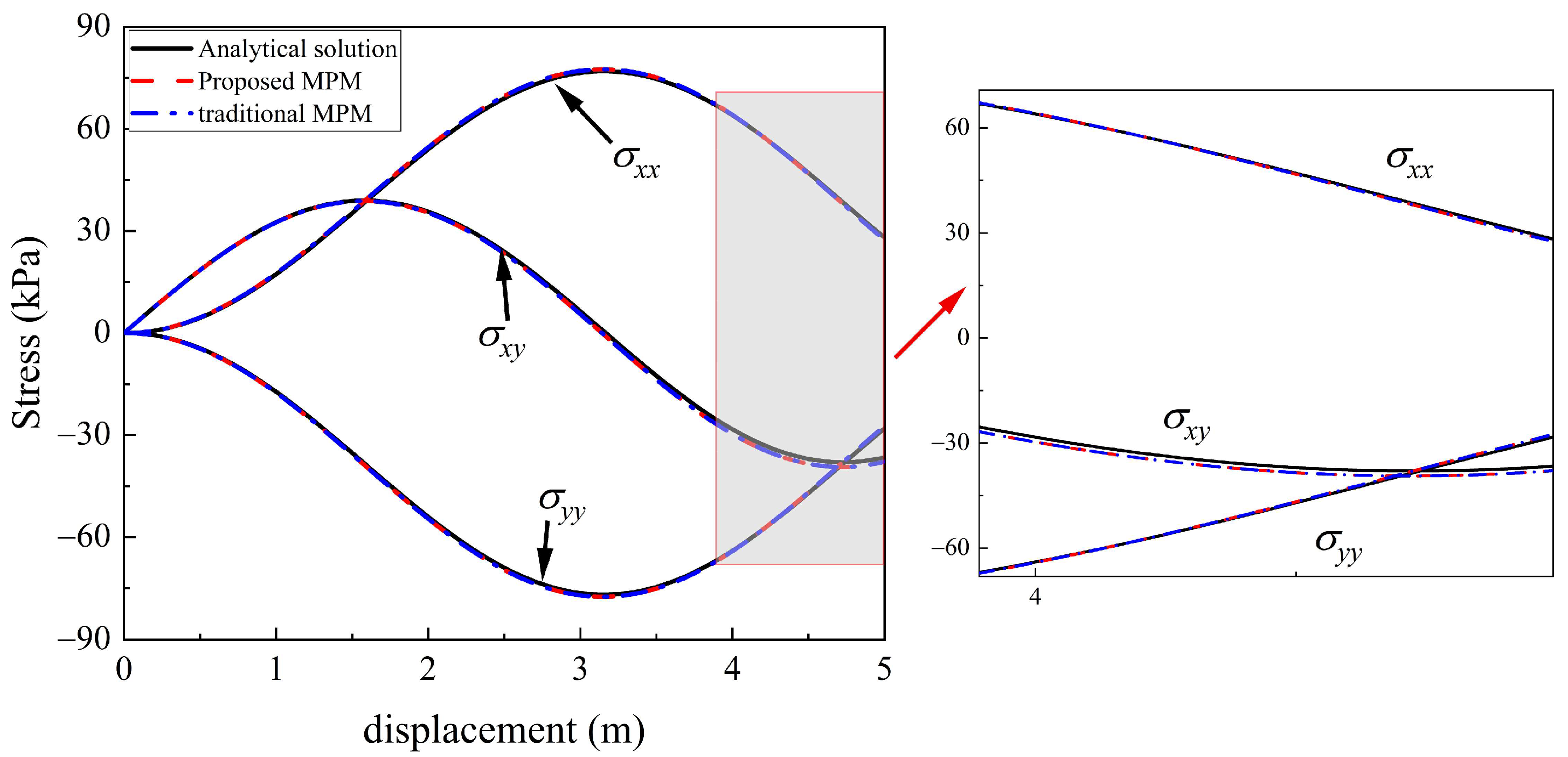
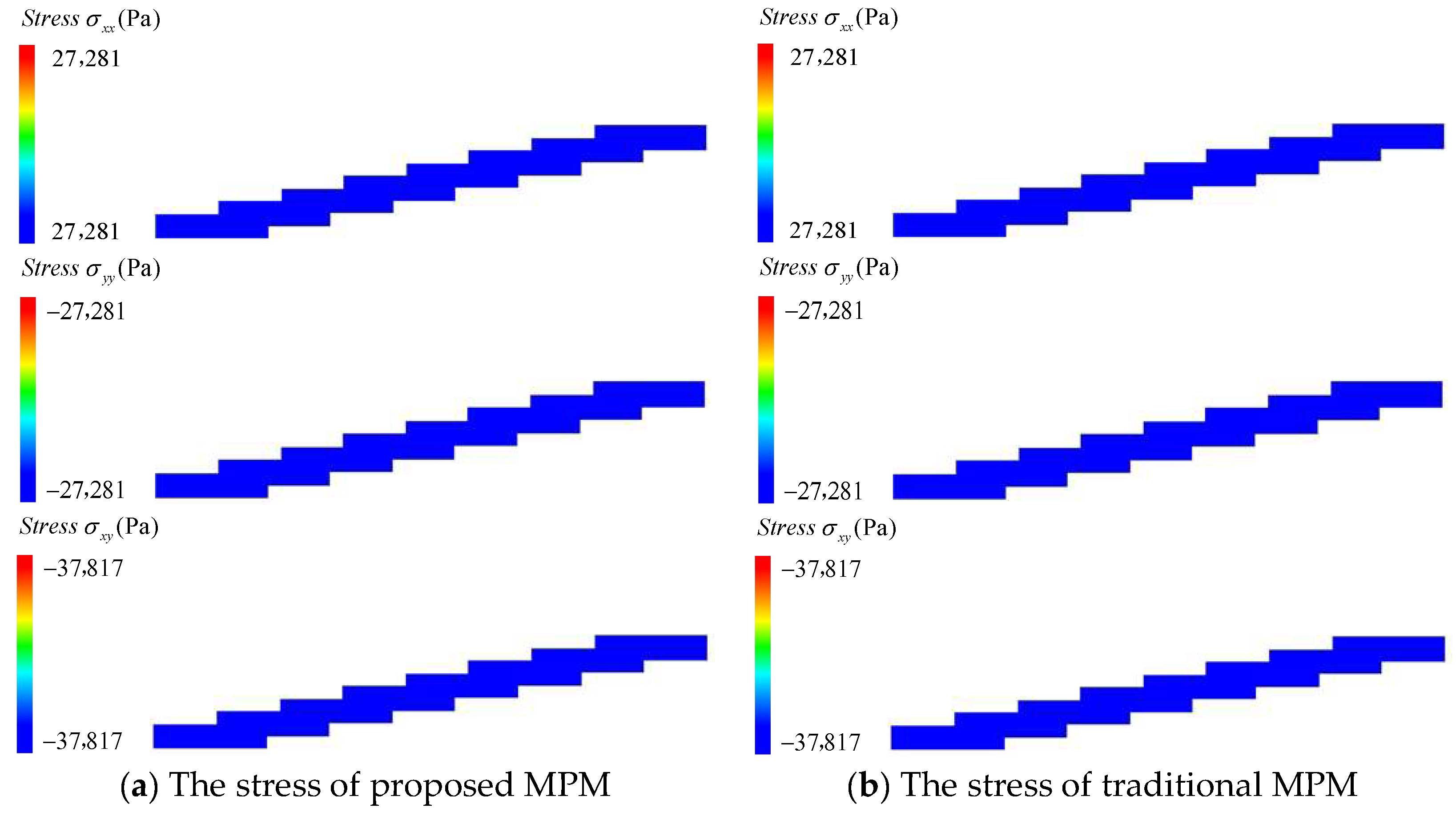
Figure 3 compares the stress and displacement responses at the center points obtained from the analytical solution, the improved material point method (MPM), and the traditional MPM. The left panel provides an overview of the entire loading process, demonstrating that both MPM variants are in good general agreement with the analytical solution, thereby validating the successful implementation of the Jaumann stress rate in the implicit MPM framework. The right panel offers a detailed view of the key region (around 4 to 5 m of displacement). In this region, the horizontal and vertical stress curves from both MPM models align closely with the analytical solutions, while minor discrepancies are observed in the shear stress curve compared to the theoretical result. Figure 4 shows the final stress distribution in the deformed body, including the horizontal, vertical, and shear stresses. All material points have consistent results throughout the model. The performance of the proposed MPM is further verified under the Dirichlet boundary condition.

5.2. Elastic Cantilever Beam

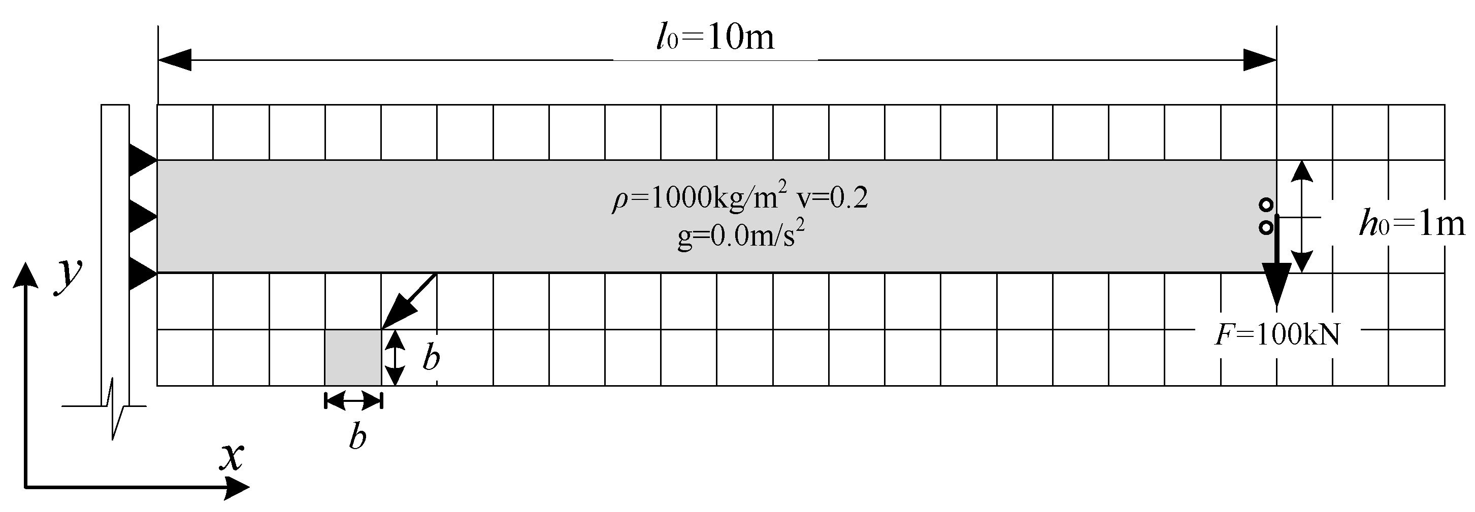
In this example, a 2D cantilever beam model is analyzed with two kinds of MPM frameworks, as shown in Figure 5. The load condition is applied with a concentrated load F = 100 kN in the vertical direction, and the acceleration g is 0.0 m/s2. The external force is applied with equal loading steps. In the simulations, the height of beam h0 is 1 m, and the length of beam l0 is 10 m. The material parameters are that the Young’s modulus is E = 12 MPa, and the Poisson’s ratio is v = 0.2.
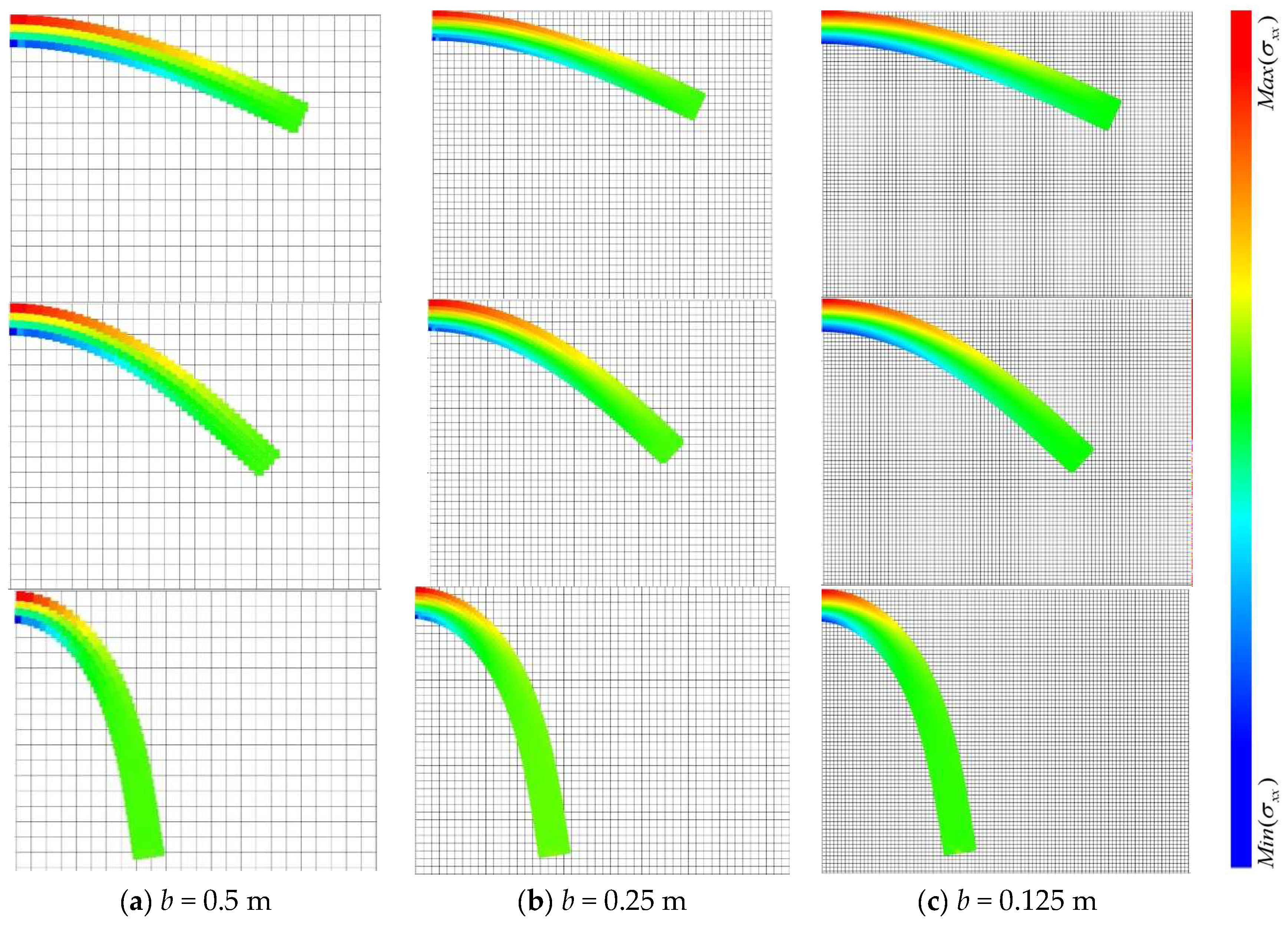
Figure 6 shows that the deformation and horizontal stress of beams are obtained by the proposed MPM with different background mesh sizes (0.5 m, 0.25 m, and 0.125 m), and four material points per element. It is evident that this is a large-deformation problem, where the vertical deformation of the beam is nearly equivalent to its original horizontal length. As the background mesh size decreases, the continuity of the stress distribution improves significantly. This improvement is primarily attributed to the use of the uGIMP and the proposed Lagrangian formulation of equilibrium within the MPM framework.
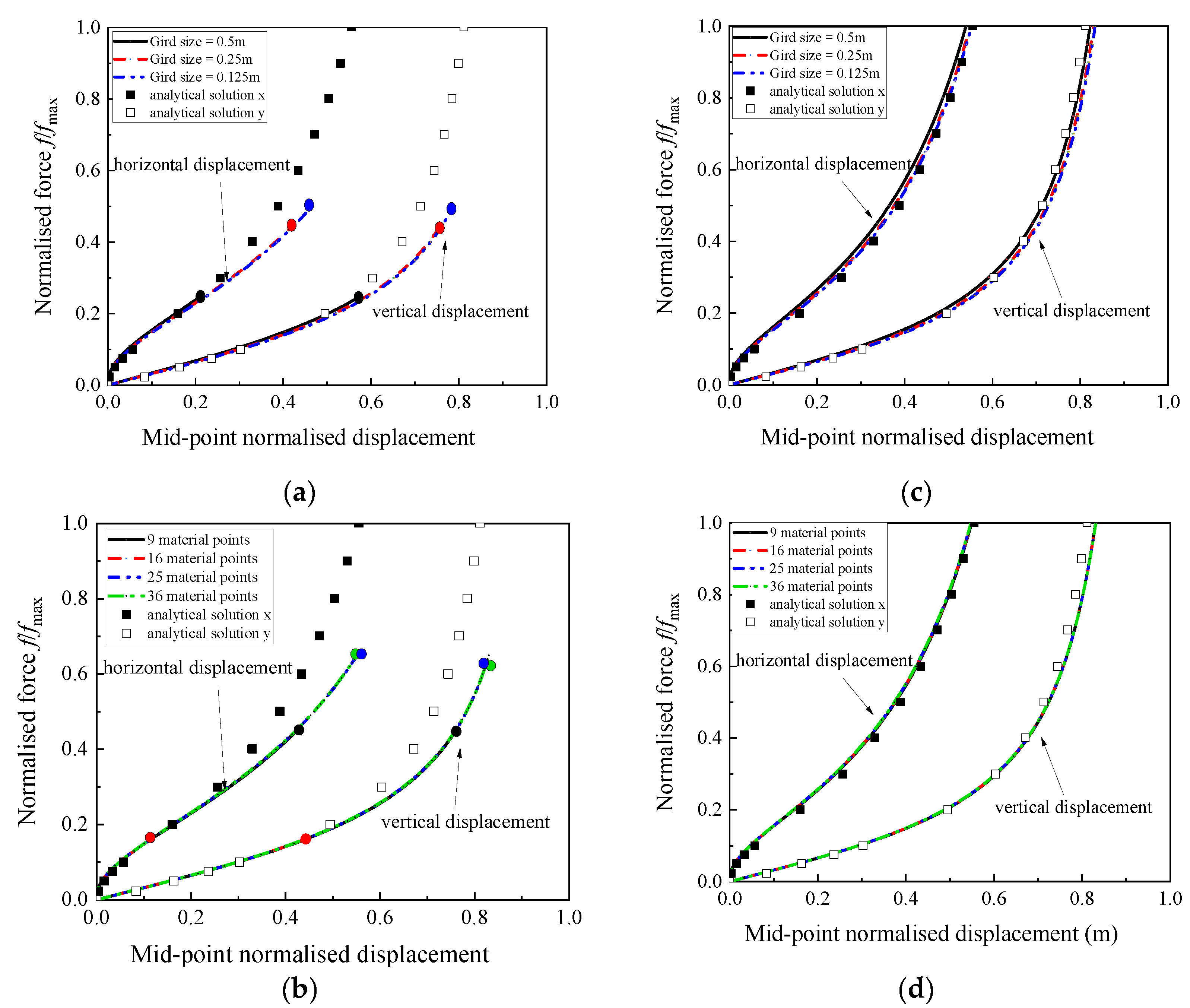
To comprehensively evaluate the robustness of the traditional and proposed MPM, Figure 7 illustrates the relationship between the normalized force and mid-point displacement for a cantilever beam, focusing on two key parameters: the size of the background grid and the number of material points per mesh. Figure 7a,c present the results of the traditional and proposed MPM, respectively. For the traditional MPM, using mesh sizes of 0.5 m, 0.25 m, and 0.125 m, the calculation fails to converge at specific loading steps (e.g., step 25, 45, and 50), demonstrating that mesh refinement does not enhance stability. In contrast, the proposed MPM maintains high stability and accuracy across all mesh sizes.
To examine the influence of the initial number of material points per mesh, a fixed background grid size of 0.25 m and 16, 25, and 36 material points per mesh is used. The results for the traditional and proposed MPM are presented in Figure 7b,d, respectively. For the traditional MPM, the displacements agree with the analytical solution only at low normalized forces (below 0.2). Under increased loading, the displacements exceed the analytical solution, and the computation fails to converge. In contrast, the proposed MPM yields results that match the analytical solution. It has minimal sensitivity to the initial number of material points, underscoring its superior reliability and insensitivity to discretization parameters.
The results clearly demonstrate that neither mesh refinement nor an increase in the number of material points per cell improves the computational stability of the traditional MPM under large-rotation deformations. This instability is primarily attributed to the omission of higher-order nonlinear terms in the equilibrium equations, which leads to an underestimation of the geometric stiffness of the deforming body and consequently results in solution inaccuracies. In contrast, the proposed UL formulation of the equilibrium equations retains these essential higher-order nonlinear terms. This ensures both accuracy and stability in simulations involving large deformations. These findings are consistent with the work of Charlton et al. [24] and Coombs et al. [25], who use finite strain assumptions in the MPM equilibrium equations to correctly capture geometric nonlinear stiffness and accurately reproduce the geometric response of cantilever beams under finite deformations.
Figure 8 presents an analysis of the deformation errors at the free end of a cantilever beam under different grid sizes and number of material points per mesh. The relative error and mean relative error are applied, which can be obtained:
e r r o r = u A , i u N , i u A , i × 100 %
M E = 1 N i = 1 N u A , i u N , i u A , i × 100 %
where error is the relative error, uA,i and uN,i are analytical solution and numerical solution of MPM, ME is the mean relative error, N is the number of data points.
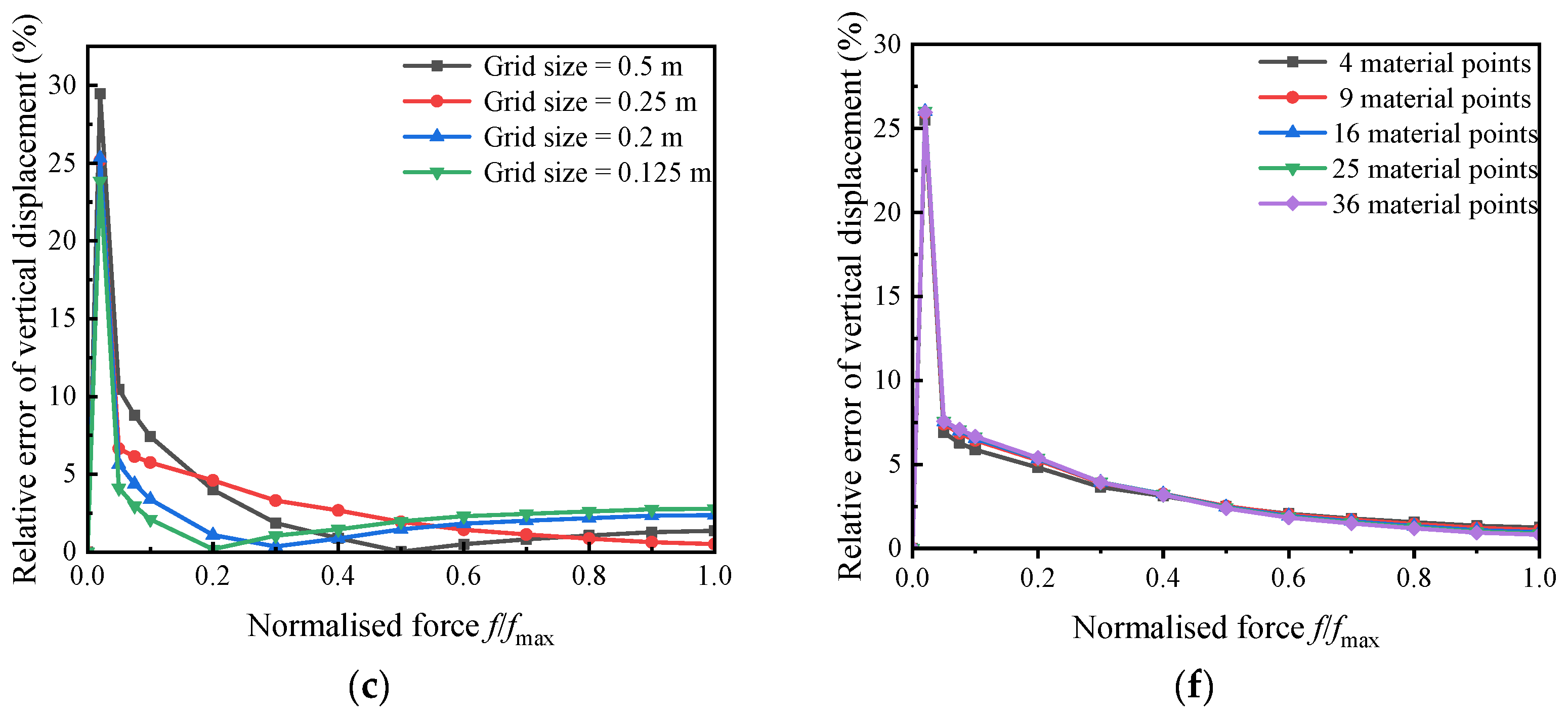
Figure 8a displays the variation in the relative error between the MPM results and the analytical solution with respect to the grid size. It can be observed that as the grid is refined from 0.5 m to 0.125 m, the mean relative error of the displacement at the beam end generally decreases in an approximately linear manner. When the grid size reaches 0.2 m, the rate of decrease in the mean relative error slows and begins to stabilize. Figure 8b,c illustrate the relationship between the relative error in horizontal and vertical displacements at the beam end and the applied external load. The relative error in both directions initially increases, peaks at a low load level (approximately 0.05), and subsequently decreases. This peak error at the early loading stage is primarily attributed to the very small displacement magnitude, which amplifies the relative error. Figure 8d shows the variation in the relative error with the number of material points per background grid cell. The results indicate that the mean relative error quickly converges to a stable value as the number of material points increases. Figure 8e,f present the relative error versus load curves under different discretization settings, where a similar trend of an initial increase followed by a decrease is observed. The numerical results stabilize with further loading. The error analysis demonstrates that the proposed MPM can accurately capture the deformation characteristics, including large rotations, in the cantilever beam problem.
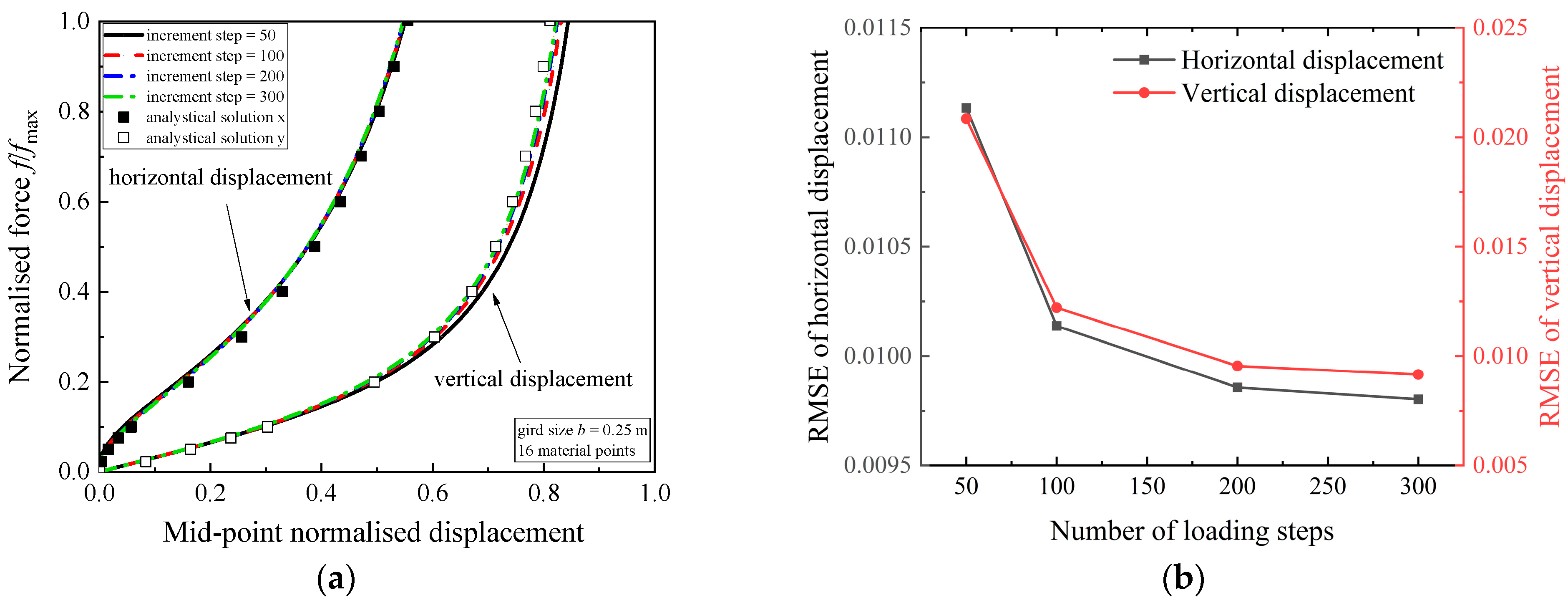
In order to further study the influence of the loading steps of the proposed approach, the external load is applied to 50, 100, and 300 steps, respectively. The background grid size b = 0.25 m and 16 material points per element are used in the model. Figure 9 shows the responses of the beam model. As shown in Figure 9a, the horizontal displacement of all cases does not clearly change, and the value of vertical displacement is closer to the analytical solution with increasing the number of loading steps. The Root Mean Square Error (RMSE) is used to analyze the influence of the calculation step size on the model calculation results, where RMSE is defined as
R M S E = 1 N i = 1 N u a , i u p , i 2
where N is the number of data point, ua,i is the analyzed displacement value, up,i is the displacement value for MPM. The corresponding RMSE of the displacement is presented in Figure 9b, which shows that the RMSE decreases as the number of loading steps increases. When the loading step reaches 200 steps, the RMSE of the horizontal and vertical displacement reaches 0.00955 and 0.00986. The result of vertical displacement begins to converge, and the RMSE also stabilizes, indicating sufficient numerical accuracy.
Figure 10 presents the number of iterative steps required by two formulations, MPM, for analyzing a cantilever beam, using a mesh size of b = 0.25 m and nine material points per element. For the traditional MPM, the number of iterations gradually increases as the simulation progresses, and the computation eventually fails to converge after the 40th step. In contrast, the proposed MPM consistently converges within four iterations throughout the entire analysis.
To quantitatively compare computational efficiency, all analyses are conducted on a computer running the Windows 10 operating system, using Fortran 2024, and equipped with a 2.1 GHz Intel Xeon Gold 6238 CPU and 256 GB of RAM. Table 2 provides a detailed runtime analysis, which is performed with a grid size of b = 0.125 m, nine material points per cell, and 40 increments to compare the two methods. Due to the similar computational workflow but a significantly reduced number of iterations required by the proposed method, it achieves substantial time savings across all major computational phases compared to the conventional MPM. Specifically, the total time for the computational model is reduced by 50.67% (from 12,516.14 ms to 6172.13 ms). Key phases, such as the computation and assembly of the stiffness matrix, show a reduction of 50.80% (from 10,671.88 ms to 5250.25 ms), and the time for updating material point information is reduced by 42.21% (from 2812.50 ms to 1625.25 ms). Similar efficiency improvements are observed in other phases, including the computation of external and internal forces (a reduction of 50.97%) and the linear solver time (a reduction of 49.23%). These results confirm that the enhanced stability of the proposed MPM directly translates into significantly higher computational efficiency.

5.3. Slope Stability Analysis

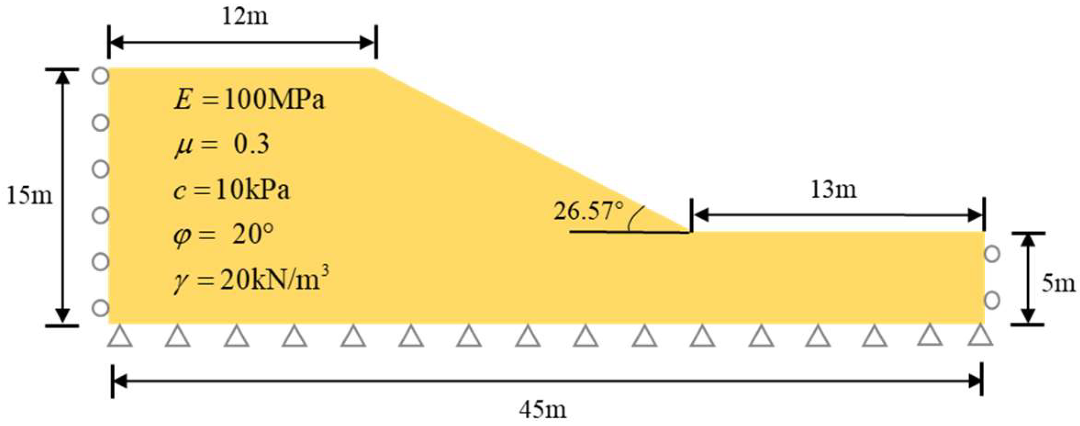
This study analyzes a homogeneous soil slope using the strength reduction method. The resulting safety factor is used to evaluate the reliability of the proposed method for solving elastoplastic problems. The geometry of the slope is illustrated in Figure 11. The material properties are defined as follows: Young’s modulus E = 100 MPa, Poisson’s ratio v = 0.3, cohesion c = 10 kPa, friction angle φ = 20°, and unit weight γ = 20 kN/m3. The bottom boundary of the slope is fully fixed, while the lateral boundaries are constrained in the horizontal direction. The Mohr–Coulomb yield criterion is adopted to characterize the material’s plastic behavior. The yield function and plastic potential function of the constitutive model are defined as follows:
F = 1 3 I 1 sin φ + cos θ σ 1 3 sin θ σ cos φ c cos φ
G = 1 3 I 1 sin ϕ + cos θ σ 1 3 sin θ σ cos ϕ c cos ϕ
where I1 is the mean stress, c is the cohesion force, φ is the friction angle, ϕ is the dilatancy angle, θ σ is the Lord angle.
Using the strength reduction method, the material cohesion c and friction angle φ are progressively reduced until slope failure occurs. The factor of safety (FOS) is then calculated based on the corresponding reduction ratio. This process can be expressed mathematically as
c = c S R F
φ = a r c tan tan φ S R F
where c and φ are the material parameters after strength reduction, and SRF is the reduction factor.
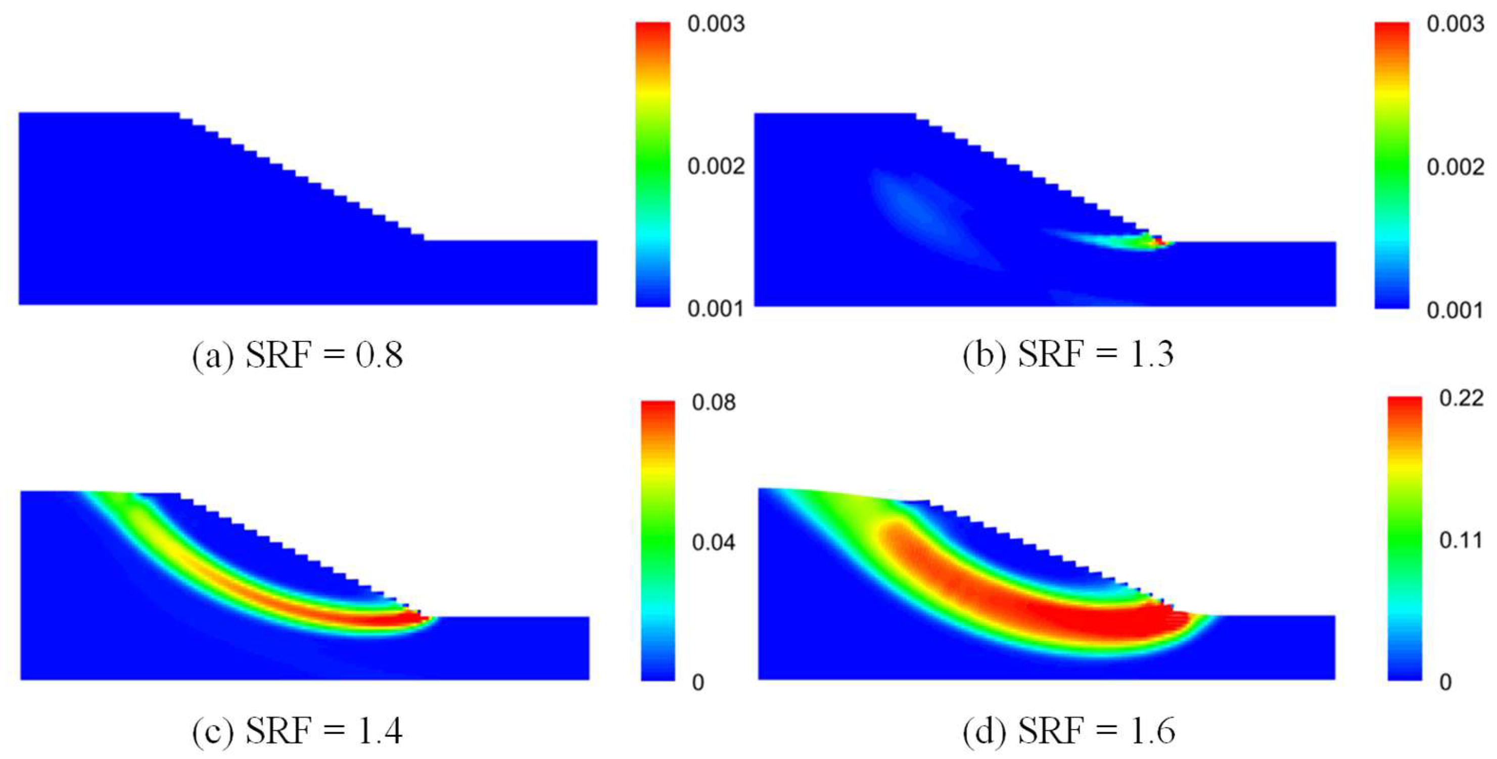
The simulation results for the reduction factor SRF, ranging from 0.8 to 1.6, are presented in Figure 12. When SRF ≤ 1.3, the maximum displacement of the slope is negligible, and the proposed MPM successfully achieves convergence of the equilibrium equations. In contrast, when SRF ≥ 1.4, the slope displacement increases continuously, and convergence cannot be achieved even after a large number of iterations (500 steps). In other words, the slope remains stable for SRF ≤ 1.3 and becomes unstable for SRF ≥ 1.4. These results indicate that the FOS lies between 1.3 and 1.4, which is in close agreement with the analytical solution of 1.38 [32].
Figure 13 illustrates the distribution of the deviatoric plastic strain invariant ε ¯ = 2 / 3 e p : e p ( e p denoting the deviatoric plastic strain tensor) in the slope under different SRFs. For SRF ≤ 1.3, the plastic strain is minimal, with localized plastic zones appearing only at the toe of the slope. When SRF = 1.4, the plastic zones coalesce to form a distinct shear band, along which the soil mass undergoes downslope movement, ultimately leading to landslide formation. This shear band development is also a well-recognized indicator of slope instability. Finally, the large-deformation case with SRF = 1.6 after 500 steps is shown in Figure 13d, where a pronounced sliding failure of the slope is observed. These results confirm the effectiveness of the proposed method in simulating large-deformation and failure processes in geotechnical problems.

5.4. Strip Footing on Undrained Soil

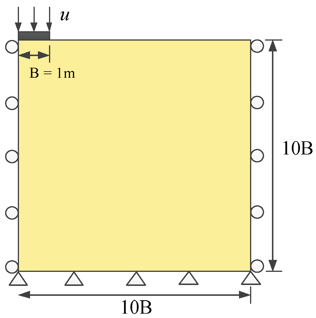
The final benchmark problem involves a plane-strain rigid strip footing [33,34], designed to evaluate the bearing capacity of weightless soil under both small- and large-deformation conditions and to demonstrate the applicability of the proposed MPM to practical geotechnical engineering problems. The geometry and boundary conditions are shown in Figure 14. Owing to symmetry, only the right half of the domain is modeled. The computational mesh is composed of linear quadrilateral elements, each containing four material points. The soil is represented as an elastic–perfectly plastic Mohr–Coulomb material following an associated flow rule. To ensure that the ultimate load capacity can be reached under small-deformation conditions, the soil parameters are specified as Young’s modulus E = 1.0 × 10⁵ kPa, Poisson’s ratio ν = 0.49, cohesion c = 1 kPa, friction angle φ = 0°, expansion angle ϕ = 0°.
In simulations of rigid strip footings, volumetric locking often arises, leading to distorted numerical results. To alleviate this problem, the present study employs the B-bar method—an approach analogous to the reduced integration scheme implemented in ABAQUS. In the two-dimensional case, a modified displacement–strain matrix, B ¯ L is used in place of the conventional matrix BL to compute particle strains and internal forces, as expressed by
B ¯ L = 1 2 N c x + N i p x 1 2 N c y N i p y 1 2 N c x N i p x 1 2 N c y + N i p y N i p y N i p x
where N c x and N c y are the gradient of interpolation functions evaluated at the center of the mesh in the x and y direction, respectively.
  • Small deformation;
In the small-deformation analysis, to validate the accuracy of the proposed MPM, a corresponding finite element model is established in ABAQUS, incorporating consistent geometry and boundary conditions with the MPM model, as illustrated in Figure 14. The computational domain is discretized using linear quadrilateral elements with reduced integration (CPE4R), with a uniform mesh size of 0.1 m. The soil is modeled as an elastic-perfectly plastic material following the Mohr–Coulomb criterion, using the same parameters as in the MPM simulations. The analysis is performed using an Implicit Static General step, with a total time of 1.0 s and an automatic analysis step size. Meanwhile, the initial step size is 0.01 s, the minimum incremental step is 1 × 10⁻⁵ s, and the maximum incremental step is 1 s. A vertical displacement of u = 0.001 m is imposed on the strip footing.
Figure 15 compares the mean stress and deviatoric plastic strain distributions obtained from the FEM, the proposed MPM incorporating the B-bar method, and the proposed MPM without B-bar treatment. It can be observed that the latter exhibits pronounced stress oscillations due to the nearly incompressible material constraints, while its deviatoric plastic strain contours display a spear-shaped pattern (Figure 15(c1,c2)). In contrast, the proposed MPM with the B-bar formulation produces results that are in close agreement with the FEM simulations. These findings demonstrate that incorporating the B-bar technique into the proposed MPM effectively mitigates volumetric locking and improves the overall accuracy of the solution.
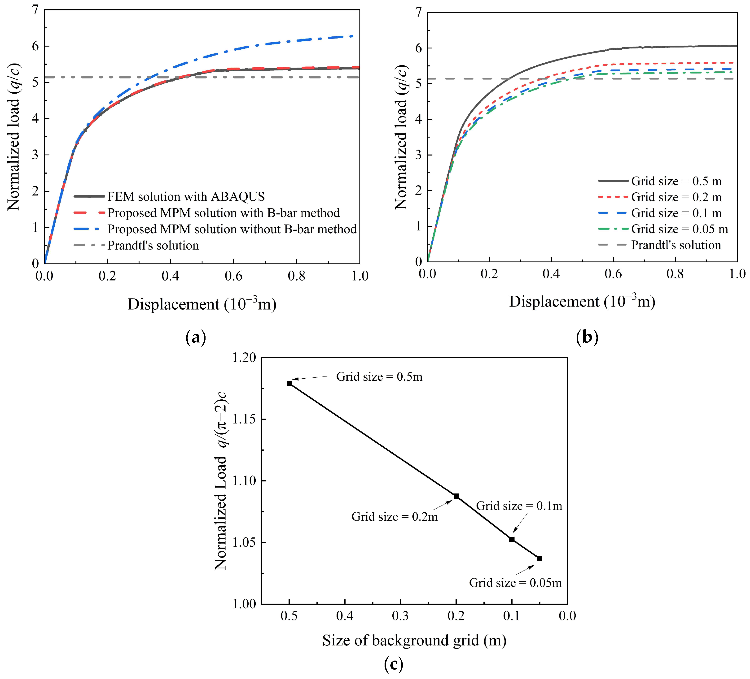
Figure 16 illustrates the response characteristics of soil under external loading. The numerical results obtained with the B-bar MPM show excellent agreement with those from the FEM. In contrast, the traditional MPM exhibits a noticeably stiffer response and fails to converge to the lower-bound solution (π + 2)c derived by Prandtl [35]. To investigate the influence of mesh size, four simulations were conducted using background grid sizes of 0.5 m, 0.2 m, 0.1 m, and 0.05 m. As observed in Figure 16b, when the mesh is refined from 0.5 m to 0.05 m, the values in the stabilized segment of the curve progressively approach the Prandtl reference solution. The convergence rate quantified in Figure 16c indicates that the numerical solution exhibits a trend of linear decrease as the mesh size reduces, while simultaneously converging toward the reference solution. These results demonstrate that the proposed MPM integrated with the B-bar technique effectively and reliably simulates the bearing behavior of soil under small deformation and incompressible conditions.
2.
Large deformation;
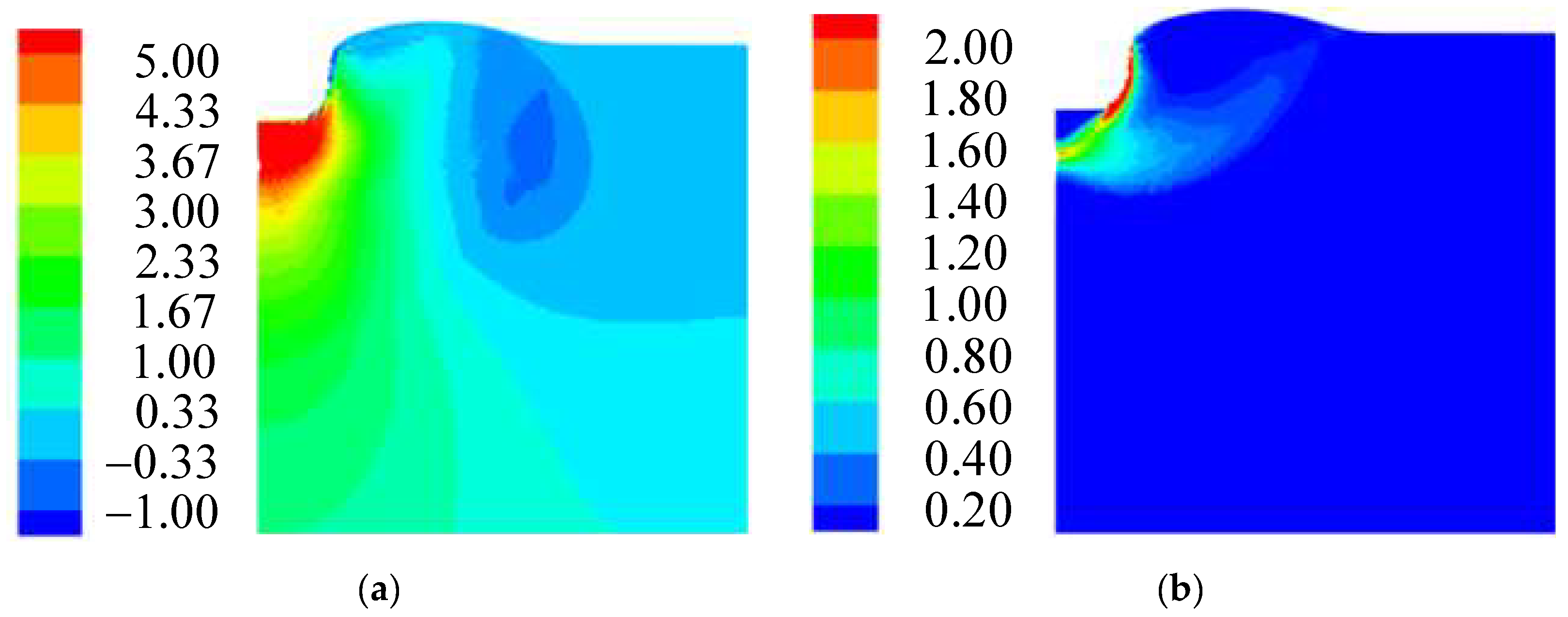
In the large-deformation analysis, the soil’s Young’s modulus is set at 100 kPa, and a vertical displacement of 1.5 m is applied over 200 load steps. All other parameters remain consistent with those employed in the small-deformation case. The vertical stress distribution derived from the proposed MPM with the B-bar method is shown in Figure 17a. The contour is smooth, free from checkerboard oscillations, with the high-stress region concentrated directly beneath the footing. Figure 17b presents the distribution of deviatoric plastic shear strain, revealing the development of significant plastic shear zones beneath and along the sides of the footing. Similar deformation and failure patterns have been reported by Jin et al. [36] and Wang et al. [37].
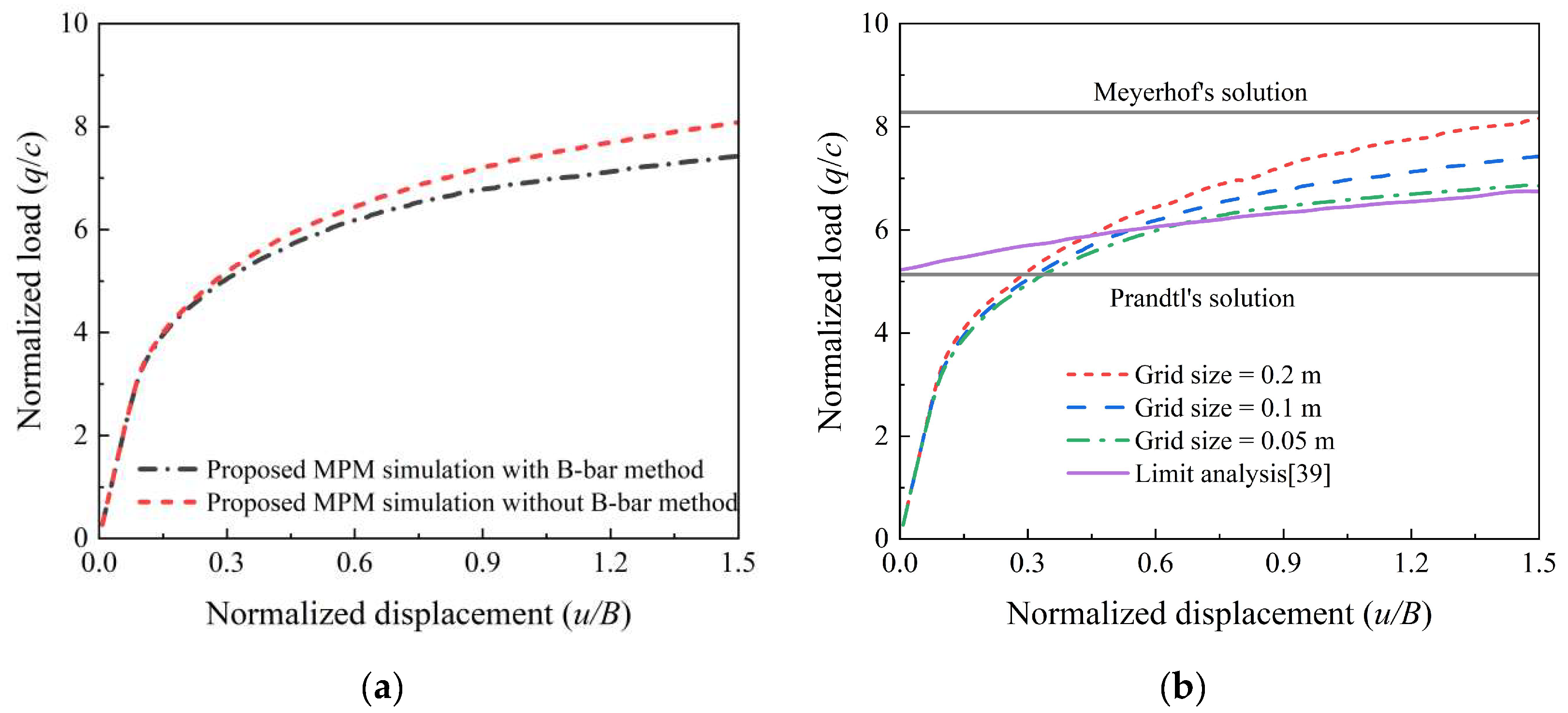
Figure 18 illustrates the normalized load–displacement responses of a rigid strip footing subjected to vertical penetration under large deformation. Figure 18a compares the performance of the proposed MPM with and without the B-bar stabilization, utilizing a fixed grid size of 0.1 m. The simulation without the B-bar method consistently overpredicts the load response, a phenomenon attributed to the spurious stiffness resulting from volumetric locking in the absence of stabilization. In contrast, the stabilized results effectively mitigate this numerical artifact. Figure 18b presents results obtained using the proposed MPM with varying grid sizes of 0.2 m, 0.1 m, and 0.05 m. These responses lie between the lower bound solution, (π + 2)c, and the upper bound solution, (2π + 2)c, as proposed by Meyerhof [38]. With grid refinement, the predicted responses progressively converge and exhibit close agreement with the limit analysis results reported by Da Silva et al. [39]. These findings support the robustness and accuracy of the proposed approach in capturing large-deformation behavior in geotechnical penetration problems.

6. Conclusions

This study presents a novel Lagrangian equilibrium formulation for the implicit MPM, aimed at improving computational stability and accuracy in large-deformation analyses. Unlike traditional UL schemes, the proposed method formulates the equilibrium equations based on the previously converged configuration. Additionally, the spatial gradient of the interpolation function is updated at each load increment through a configuration mapping technique. To enhance numerical performance further, high-order interpolation functions are integrated to reduce cell-crossing errors, while the B-bar method is employed to alleviate volumetric locking.
The method is initially validated against analytical solutions for a simple shear problem, demonstrating excellent agreement. Its robustness is further examined through large-deformation benchmarks, such as a cantilever beam subjected to concentrated loading, where the proposed formulation exhibits superior stability and convergence compared to established approaches. Additionally, the framework is applied to representative geotechnical problems, such as slope stability analysis using the strength reduction method and strip footing simulations under both small and large deformation regimes. In these applications, the method effectively captures key failure mechanisms, shear band development, and load–displacement responses, showing consistently aligning with results from finite element simulations and limit analysis. Overall, the presented Lagrangian equilibrium formulation significantly expands the applicability of implicit MPM for simulating elastoplastic large-deformation problems, providing a reliable and accurate numerical tool for geotechnical engineering applications.
Although the proposed implicit MPM framework is demonstrated herein only under quasi-static and plane strain conditions, the UL formulation it employs has been proven applicable to dynamic conditions and three-dimensional problems in the context of the FEM [40]. Consequently, extending the present implicit MPM framework to dynamic loading and full three-dimensional simulations constitutes a key direction for future work.

Author Contributions

Conceptualization, Q.-Y.S. and Y.-L.X.; methodology, Q.-Y.S. and Z.-G.L.; software, Q.-Y.S. and Y.-L.X.; validation, Y.-L.X. and R.-X.W.; formal analysis, Q.-Y.S. and R.-X.W.; investigation, Q.-Y.S. and Z.-G.L.; resources, Q.-Y.S., J.-H.Y. and Y.-L.X.; data curation, Q.-Y.S.; writing—original draft preparation, Q.-Y.S. and Z.-G.L.; writing—review and editing, Y.-L.X., J.-H.Y. and Z.-G.L.; project administration, Q.-Y.S.; funding acquisition, Q.-Y.S. All authors have read and agreed to the published version of the manuscript.

Funding

This research was funded by the Talent Introduction Research Project of Ningbo Polytechnic, grant number NZ25RC018. National Scientific Research Project Cultivation Project by Ningbo Polytechnic, grant number NZ22GJ007.

Data Availability Statement

The original contributions presented in this study are included in the article. Further inquiries can be directed to the corresponding author.

Acknowledgments

The authors appreciate the anonymous reviewers for their constructive comments and suggestions that significantly improved the quality of this manuscript.

Conflicts of Interest

The authors declare no conflicts of interest.

Abbreviations

SymbolDescription
S t + Δ t The second PK stress tensor at time t + Δt
δεThe strain tensor corresponding to the virtual displacements
δuthe virtual displacement tensor
τTraction on the boundary surface Γ
ΓBoundary surface
bBody load vector
VVolume of continuity
CMaterial stress–strain tensor
ΔεIncremental strain tensor
δ e Linear strain tensor corresponding to the virtual displacements
δ η Nonlinear strain tensor corresponding to the virtual displacements
C JTangent modulus matrix
( · ) Gradient of quantity
K mat Material stiffness matrix
K geo Geometric stiffness matrix
BLLinear strain–displacement matrix
BNLNonlinear strain–displacement matrix
VpVolume of material point
npNumber of material points
σ ¯ Stress matrix for geometric stiffness matrix
fextExternal load vector
NipInterpolation function
hpCharacteristic length of particle
δukIterative displacement vector
kNumber iterative
ρ Mass density
P ¯ Nominal stress tensor
FDeformation gradient tensor
JDeterminant of Jacobian matrix
qTractions vector
ΔqTractions increment vector
ΔbBody force increment vector
tTime
ΔtIncrement time
P ¯ ˙ t + Δ t Nominal stress rate at the current time t + Δt
δ u ˙ Virtual velocity tensor
σ ˙ Cauchy stress rate tensor
σ t Cauchy stress tensor at time t
B ¯ N L Nonlinear strain–displacement matrix in the proposed framework
K ¯ m a t Material matrix in the proposed framework
K ¯ g e o Geometric matrix in the proposed framework
LVelocity gradient tensor
D = 1 2 L + L T Deformation rate tensor
W = 1 2 L L T Rotation tensor
tr(·)Trace of tensor
σ ˙ J Jaumann stress rate tensor
σ ¯ * Stress tensor for geometric stiffness matrix
f ¯ e x t External load on the nodes
L2-norm of the entire residual vector
ferrorResidual force vector
EYoung’s modulus
vPoisson’s ratio
Fyield function
Gplastic potential function
cCohesion force
ϕFriction angle
φDilatancy angle

Appendix A. Transformation Process of Governing Equation

The governing equation of the proposed MPM can be expressed as
V t δ L T C J : D + t r D σ t σ t L T + W σ t σ t W Δ t d V = V t δ u ˙ T ρ Δ b d V + Γ t δ u ˙ T Δ q d
In the plane strain problem, the governing equation is discretized and transformed into matrix form. The first term on the left of Equation (A1) is contributed from the material behavior, this integral is calculated as a summation of particles:
V t δ L T C J : D d V Δ t = δ u ˙ T V t N i p x T C J : D Δ t d V = δ u ˙ T p = 1 n B L T C J B L u ˙ Δ t V p = δ u ˙ T K ¯ m a t Δ u
K ¯ m a t = p = 1 n B L T C J B L V p
where u ˙ is the velocity vector, K ¯ m a t is the material stiffness matrix, CJ is the fourth-order material behavior tensor, BL is the linear strain–displacement matrix, can be written as
B L = N i p 1 x 0 N i p n x 0 0 N i p 1 y 0 N i p n y N i p 1 y N i p 1 x N i p n y N i p n x
The geometric nonlinear term of governing equation is
V t δ L T t r D σ t σ t L T Δ t d V = V t δ L T σ 11 t σ 11 t 0 0 σ 22 t σ 22 t 0 0 σ 12 t σ 12 t 0 0 σ 21 t σ 21 t 0 0 L Δ t δ L T σ 11 t 0 σ 12 t 0 0 σ 22 t 0 σ 12 t 0 σ 12 t 0 σ 11 t σ 12 t 0 σ 22 t 0 L Δ t d V = V t δ L T 0 σ 11 t σ 12 t 0 σ 22 t 0 0 σ 12 t σ 12 t 0 0 σ 11 t 0 σ 12 t σ 22 t 0 L Δ t d V = δ u ˙ p = 1 n B ¯ N L T σ ¯ t B ¯ N L V p u ˙ Δ t
where B ¯ N L is the non-linear strain–displacement matrix, as shown in Equation (A6)
B ¯ N L = N i p 1 x 0 N i p n x 0 0 N i p 1 y 0 N i p n y N i p 1 y 0 N i p n y 0 0 N i p 1 x 0 N i p n x
To suppress the influence of rigid body rotation on the large deformation, the Jaumann stress rate is incorporated into the geometric nonlinearity. Accordingly, the geometric stiffness matrix in the governing equation can be formulated as
V t δ L T t r D σ t σ t L T + W σ t σ t W Δ t d V = V t δ L T 0 σ 11 t 0 σ 12 t σ 22 t 0 σ 12 t 0 σ 12 t 0 1 2 σ 11 t σ 22 t 1 2 σ 11 t + σ 22 t 0 σ 12 t 1 2 σ 11 t + σ 22 t 1 2 σ 11 t σ 22 t L Δ t d V = δ u ˙ p = 1 n B ¯ N L T σ ¯ t B ¯ N L V p u ˙ Δ t = δ u ˙ K ¯ g e o Δ u
K ¯ g e o = p = 1 n B ¯ N L T σ ¯ t B ¯ N L V p

References

  1. Lucy, L.B. A Numerical Approach to the Testing of the Fission Hypothesis. Astron. J. 1977, 82, 1013. [Google Scholar] [CrossRef]
  2. Belytschko, T.; Gu, L.; Lu, Y.Y. Fracture and Crack Growth by Element Free Galerkin Methods. Model. Simul. Mater. Sci. Eng. 1994, 2, 519–534. [Google Scholar] [CrossRef]
  3. Oñate, E.; Idelsohn, S.R.; Del Pin, F.; Aubry, R. The particle finite element method—An overview. Int. J. Comput. Methods 2004, 1, 267–307. [Google Scholar] [CrossRef]
  4. Liu, S.; Tang, X.; Li, J. Extension of ALE Method in Large Deformation Analysis of Saturated Soil under Earthquake Loading. Comput. Geotech. 2021, 133, 104056. [Google Scholar] [CrossRef]
  5. Sulskya, D.; Chenb, Z.; Schreyer, H.L. A Particle Method for History-Dependent Materials. Comput. Methods Appl. Mech. Eng. 1994, 118, 179–196. [Google Scholar] [CrossRef]
  6. Jiang, C.; Schroeder, C.; Selle, A.; Teran, J.; Stomakhin, A. The Affine Particle-in-Cell Method. ACM Trans. Graph. 2015, 34, 1–10. [Google Scholar] [CrossRef]
  7. Brackbill, J.U.; Ruppel, H.M. FLIP: A Method for Adaptively Zoned, Particle-in-Cell Calculations of Fluid Flows in Two Dimensions. J. Comput. Phys. 1986, 65, 314–343. [Google Scholar] [CrossRef]
  8. Bardenhagen, S.G.; Kober, E.M. The Generalized Interpolation Material Point Method. Comput. Model. Eng. Sci. 2004, 5, 477–496. [Google Scholar]
  9. Steffen, M.; Kirby, R.M.; Berzins, M. Analysis and Reduction of Quadrature Errors in the Material Point Method (MPM). Int. J. Numer. Methods Eng. 2008, 76, 922–948. [Google Scholar] [CrossRef]
  10. Sadeghirad, A.; Brannon, R.M.; Burghardt, J. A Convected Particle Domain Interpolation Technique to Extend Applicability of the Material Point Method for Problems Involving Massive Deformations. Int. J. Numer. Methods Eng. 2011, 86, 1435–1456. [Google Scholar] [CrossRef]
  11. Zhang, D.Z.; Ma, X.; Giguere, P.T. Material Point Method Enhanced by Modified Gradient of Shape Function. J. Comput. Phys. 2011, 230, 6379–6398. [Google Scholar] [CrossRef]
  12. De Koster, P.; Tielen, R.; Wobbes, E.; Möller, M. Extension of B-Spline Material Point Method for Unstructured Triangular Grids Using Powell–Sabin Splines. Comput. Part Mech. 2021, 8, 273–288. [Google Scholar] [CrossRef]
  13. Hu, Y.; Fang, Y.; Ge, Z.; Qu, Z.; Zhu, Y.; Pradhana, A.; Jiang, C. A Moving Least Squares Material Point Method with Displacement Discontinuity and Two-Way Rigid Body Coupling. ACM Trans. Graph. 2018, 37, 1–14. [Google Scholar] [CrossRef]
  14. Sulsky, D.; Schreyer, H.L. Axisymmetric Form of the Material Point Method with Applications to Upsetting and Taylor Impact Problems. Comput. Methods Appl. Mech. Eng. 1996, 139, 409–429. [Google Scholar] [CrossRef]
  15. Dong, Y.; Wang, D.; Randolph, M.F. Quantification of Impact Forces on Fixed Mudmats from Submarine Landslides Using the Material Point Method. Appl. Ocean Res. 2020, 102, 102227. [Google Scholar] [CrossRef]
  16. Cui, X.X.; Zhang, X.; Zhou, X.; Liu, Y.; Zhang, F. A Coupled Finite Difference Material Point Method and Its Application in Explosion Simulation. Comput. Model. Eng. Sci. 2014, 98, 565–599. [Google Scholar]
  17. Wang, Y.; Beom, H.G.; Sun, M.; Lin, S. Numerical Simulation of Explosive Welding Using the Material Point Method. Int. J. Impact Eng. 2011, 38, 51–60. [Google Scholar] [CrossRef]
  18. Raymond, S.J.; Jones, B.D.; Williams, J.R. Fracture Shearing of Polycrystalline Material Simulations Using the Material Point Method. Comput. Part Mech. 2021, 8, 259–272. [Google Scholar] [CrossRef]
  19. Andersen, S.; Andersen, L. Modelling of Landslides with the Material-Point Method. Comput. Geosci. 2010, 14, 137–147. [Google Scholar] [CrossRef]
  20. Llano-Serna, M.A.; Farias, M.M.; Pedroso, D.M. An Assessment of the Material Point Method for Modelling Large Scale Run-out Processes in Landslides. Landslides 2016, 13, 1057–1066. [Google Scholar] [CrossRef]
  21. Shi, Y.H.; Guo, N.; Yang, Z.X. GeoTaichi: A Taichi-Powered High-Performance Numerical Simulator for Multiscale Geophysical Problems. Comput. Phys. Commun. 2024, 301, 109219. [Google Scholar] [CrossRef]
  22. Wang, B.; Vardon, P.J.; Hicks, M.A.; Chen, Z. Development of an Implicit Material Point Method for Geotechnical Applications. Comput. Geotech. 2016, 71, 159–167. [Google Scholar] [CrossRef]
  23. Yuan, W.; Wang, H.; Liu, K.; Zhang, W.; Wang, D.; Wang, Y. Analysis of Large Deformation Geotechnical Problems Using Implicit Generalized Interpolation Material Point Method. J. Zhejiang Univ.-Sci. A 2021, 22, 909–923. [Google Scholar] [CrossRef]
  24. Charlton, T.J.; Coombs, W.M.; Augarde, C.E. iGIMP: An Implicit Generalised Interpolation Material Point Method for Large Deformations. Comput. Struct. 2017, 190, 108–125. [Google Scholar] [CrossRef]
  25. Coombs, W.M.; Augarde, C.E.; Brennan, A.J.; Brown, M.J.; Charlton, T.J.; Knappett, J.A.; Ghaffari Motlagh, Y.; Wang, L. On Lagrangian Mechanics and the Implicit Material Point Method for Large Deformation Elasto-Plasticity. Comput. Methods Appl. Mech. Eng. 2020, 358, 112622. [Google Scholar] [CrossRef]
  26. Coombs, W.M.; Augarde, C.E. AMPLE: A Material Point Learning Environment. Adv. Eng. Softw. 2020, 139, 102748. [Google Scholar] [CrossRef]
  27. González Acosta, J.L.; Vardon, P.J.; Hicks, M.A. Development of an Implicit Contact Technique for the Material Point Method. Comput. Geotech. 2021, 130, 103859. [Google Scholar] [CrossRef]
  28. Li, S.; Zhang, Y.; Wu, J.; Yu, J.; Gong, X. Modeling of Crack Propagation with the Quasi-Static Material Point Method. Eng. Fract. Mech. 2021, 245, 107602. [Google Scholar] [CrossRef]
  29. Oka, F.; Yashima, A.; Shibata, T.; Kato, M.; Uzuoka, R. FEM-FDM Coupled Liquefaction Analysis of a Porous Soil Using an Elasto-Plastic Model. Appl. Sci. Res. 1994, 52, 209–245. [Google Scholar] [CrossRef]
  30. Flanagan, D.P.; Taylor, L.M. An Accurate Numerical Algorithm for Stress Integration with Finite Rotations. Comput. Methods Appl. Mech. Eng. 1987, 62, 305–320. [Google Scholar] [CrossRef]
  31. Dienes, J.K. On the Analysis of Rotation and Stress Rate in Deforming Bodies. Acta Mech. 1979, 32, 217–232. [Google Scholar] [CrossRef]
  32. Bishop, A.W.; Morgenstern, N. Stability Coefficients for Earth Slopes. Géotechnique 1960, 10, 129–153. [Google Scholar] [CrossRef]
  33. Sołowski, W.T.; Sloan, S.W. Evaluation of Material Point Method for Use in Geotechnics. Int. J. Numer. Anal. Methods Geomech. 2015, 39, 685–701. [Google Scholar] [CrossRef]
  34. Xie, M.; Navas, P.; López-Querol, S. An Implicit Locking-free B-spline Material Point Method for Large Strain Geotechnical Modelling. Int. J. Numer. Anal. Methods Geomech. 2023, 47, 2741–2761. [Google Scholar] [CrossRef]
  35. Ludwig Prandtl Über Die Härte Plastischer Körper. Nachrichten Von Ges. Wiss. Zu Gött. Math. Phys. Kl. 1921, 1, 15–20.
  36. Jin, Y.-F.; Yin, Z.-Y.; Li, J.; Dai, J.-G. A Novel Implicit Coupled Hydro-Mechanical SPFEM Approach for Modelling of Delayed Failure of Cut Slope in Soft Sensitive Clay. Comput. Geotech. 2021, 140, 104474. [Google Scholar] [CrossRef]
  37. Wang, Z.; Jin, Y.; Yin, Z.; Wang, Y. A Novel Coupled NS-PFEM with Stable Nodal Integration and Polynomial Pressure Projection for Geotechnical Problems. Int. J. Numer. Anal. Methods Geomech. 2022, 46, 2535–2560. [Google Scholar] [CrossRef]
  38. Meyerhof, G.G. The Ultimate Bearing Capacity of Foudations. Géotechnique 1951, 2, 301–332. [Google Scholar] [CrossRef]
  39. da Silva, M.V.; Krabbenhoft, K.; Lyamin, A.V.; Sloan, S.W. Rigid-plastic Large-deformation Analysis of Geotechnical Penetration Problems. Proceedings of 13th IACMAG conference. Comput Methods Geomech Front New Appl. 2011, 1, 42–47. [Google Scholar]
  40. Ye, B.; Ye, G.; Zhang, F.; Yashima, A. Experiment and Numerical Simulation of Repeated Liquefaction-Consolidation of Sand. Soils Found. 2007, 47, 547–558. [Google Scholar] [CrossRef]
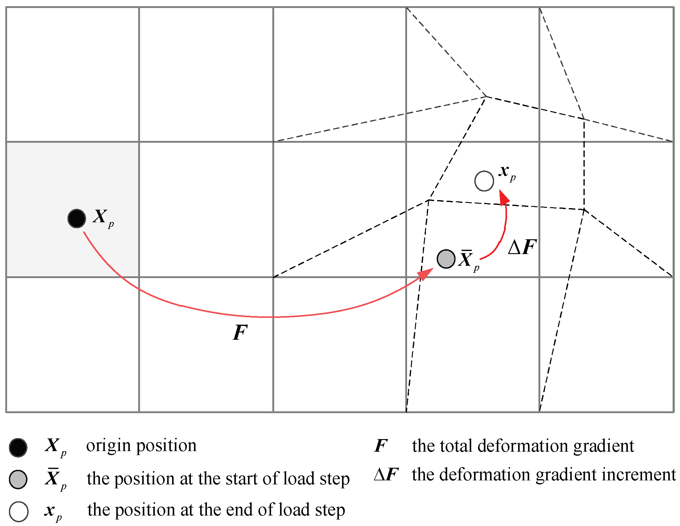
Figure 1. The deformation of a material point from the reference to the current configuration.
Symmetry 17 01876 g001
Figure 2. Simple shear model.
Symmetry 17 01876 g002
Figure 3. The relationship between the stress and normalized displacement for analytical solution, traditional MPM, and proposed MPM.
Symmetry 17 01876 g003
Figure 4. The stress distribution for traditional MPM and proposed MPM with Jaumann stress rate tensor. (a) the result using the proposed MPM; (b) the result using the traditional MPM.
Symmetry 17 01876 g004
Figure 5. Schematic diagram of beam model.
Symmetry 17 01876 g005
Figure 6. The horizontal stress σxx of beam for load steps 5, 20, and 100. (a) grid size b = 0.5 m; (b) grid size b = 0.25 m; (c) grid size b = 0.125 m.
Symmetry 17 01876 g006
Figure 7. The relationship between the normalized force and mid-point displacement at different sizes of background grid. (a) the result using the traditional MPM with different numbers of material points; (b) the result using the proposed MPM with different numbers of material points; (c) the result using the traditional MPM with different grid sizes; (d) the result using the proposed MPM with different grid sizes.
Symmetry 17 01876 g007
Figure 8. Analysis of the deformation errors using the proposed MPM at the free end of a cantilever beam under different grid sizes and number of material points per mesh. (a) Mean relative error of displacement under different gird sizes; (b) relative error of horizontal displacement under different gird sizes; (c) relative error of vertical displacement under different gird sizes; (d) mean relative error of displacement under different number of material points per mesh; (e) relative error of horizontal displacement under different number of material points per mesh; (f) relative error of vertical displacement under different number of material points per mesh.
Symmetry 17 01876 g008aSymmetry 17 01876 g008b
Figure 9. The relationship between the normalized force and mid-point displacement (The background grid size b = 0.25 m and 16 material points used in each grid), (a) different loading steps, (b) RMSE of displacement with different loading steps.
Symmetry 17 01876 g009
Figure 10. The number of iterative steps for two kinds of MPM.
Symmetry 17 01876 g010
Figure 11. Homogeneous slope model.
Symmetry 17 01876 g011
Figure 12. Maximum displacement of the slope.
Symmetry 17 01876 g012
Figure 13. The plastic strain invariant of the slope: (a) SRF = 0.8, (b) SRF = 1.3, (c) SRF = 1.4, and (d) SRF = 1.6.
Symmetry 17 01876 g013
Figure 14. The strip footing model.
Symmetry 17 01876 g014
Figure 15. Mean stress and deviatoric plastic strain contours of a rigid strip footing under vertical penetration at small deformation (grid size b = 0.1 m), (a1,a2) FEM solution; (b1,b2) proposed MPM with B-bar method; (c1,c2) proposed MPM without B-bar method.
Symmetry 17 01876 g015
Figure 16. Normalized load–displacement responses of a rigid strip footing under vertical penetration at small deformation: (a) comparison between results obtained from the FEM and the proposed MPM (grid size = 0.1 m); (b) the vertical displacement-load curve via the B-bar method with different grid sizes; (c) convergence rate for the proposed MPM.
Symmetry 17 01876 g016
Figure 17. The contours of a rigid strip footing using the proposed MPM with B-bar method under vertical penetration at large deformation (grid size b = 0.1 m), (a) vertical stress contour (kPa); (b) deviatoric plastic strain contour.
Symmetry 17 01876 g017
Figure 18. Normalized load–displacement responses of a rigid strip footing under vertical penetration at large deformation: (a) comparison between results obtained from the proposed MPM with B-bar method and the proposed MPM with B-bar method (grid size b = 0.1 m); (b) convergence characteristics computed via the B-bar method with different grid sizes (grid size b = 0.2, 0.1, 0.05 m) [39].
Symmetry 17 01876 g018
Table 1. Comparison of key quantities required for the implicit MPM framework.
ReferenceFormulationBasic AssumptionObjective Stress RateConfigurationUpdated Interpolation Function Gradient
Wang et al. [22]ULSmall strainJaumann stress rateCurrent configuration/
Yuan et al. [23]ULSmall strainJaumann stress rateCurrent configuration/
Acosta et al. [27]ULSmall strain/Current configuration/
Li et al. [28]ULSmall strain/Current configuration/
Charlton et al. [24]ULLarge strain/Current configurationMapping configuration method
Coombs et al. [26]Novel LagrangianLarge strain/Previous configuration/
The proposed
MPM
ULSmall strainJaumann stress ratePrevious configurationMapping configuration method
Note: “/” indicates not used or not mentioned in the paper.
Table 2. Elastic beam: Comparison of run time distribution for the proposed MPM and traditional MPM with b = 0.125 m and nine material points per mesh.
Calculation ProcessProposed MPM (ms)Traditional MPM (ms)Relative Error (%)
Initialization578.125578.1250.0
Computational model6172.1312,516.1450.67
Stiffness matrix calculation and assembly5250.2510,671.8850.80
External and internal force406.25828.6350.97
Linear solver515.631015.6349.23
Update the information of material point (e.g., displacement, deformation gradient, strain, stress and so on)1625.252812.5042.21
Note: The blue-filled cells are sub-calculations of the numbered entries.
Disclaimer/Publisher’s Note: The statements, opinions and data contained in all publications are solely those of the individual author(s) and contributor(s) and not of MDPI and/or the editor(s). MDPI and/or the editor(s) disclaim responsibility for any injury to people or property resulting from any ideas, methods, instructions or products referred to in the content.