Article

An Online Reduced KPLS Data-Driven Method for Fault Diagnosis of Nonlinear Processes

1
Research Laboratory of Automation (LARA), National Engineering School of Tunis, University of Manar, Tunis 1002, Tunisia
2
Faculty of Computers and Information Technology, University of Tabuk, Tabuk 71491, Saudi Arabia
3
Applied College, University of Tabuk, Tabuk 71491, Saudi Arabia
*
Author to whom correspondence should be addressed.
Symmetry 2025, 17(11), 1863; https://doi.org/10.3390/sym17111863
Submission received: 10 September 2025 / Revised: 11 October 2025 / Accepted: 31 October 2025 / Published: 4 November 2025
(This article belongs to the Special Issue Fault Diagnosis and Electronic Engineering in Symmetry)

Abstract

System security is a very important organizational task for the system to maintain proper functioning and to prevent modifications or hijacking of the system. Indeed, it is necessary to address any detected problem or defect to protect human beings, industry, and machines. So the identification, after the fault detection phase, of the variables correlated to the detected or occurred fault is a very important step. For this purpose, this paper proposes a nonlinear machine learning method for fault diagnosis. Indeed, the Reduced Kernel Partial Least Squares (RKPLS) is proposed as a processing method for the suitable localization of detected faults. The idea of this approach is to generate partial RKPLS models, using the principle of structured symmetry residues, with reduced sets of variables. On the other hand, the Fault Isolation (FI) using the online RKPLS method (ORKPLS) is developed in this article to generate indices of fault detection sensitive to certain faults and insensitive to others. Thus, a partial ORKPLS method, for fault isolation, is proposed to secure the systems and ensure a proper operation. The suggested approaches are applied for monitoring the continuous stirred tank reactor (CSTR) and the Air quality monitoring network (AIRLOR). The obtained results underscore the role of leveraging symmetry in designing fault.

1. Introduction

Over the years, system security has become a very important task to primarily guarantee human health and ensure the proper functioning of systems and daily life. The continued operation of systems in good condition is important to ensure a comfortable life. The authors of [1] confirmed the importance of process safety and the need to move towards the area of safety, risk and reliability. For industrial systems, defects and false identifications can, at any time, lead to poor production quality and serious process safety accidents. In this context, several researchers are working to develop new techniques and approaches to improve security and solve problems related to the detection and identification of defects, such as the center for Risk, Integrity and Safety Engineering.
The technology of fault diagnosis plays a remarkable role in ensuring the safe operation of industrial systems and has given a great attention in several searches [2,3]. Indeed, the field of fault detection and diagnosis in terms of process and industrial safety always consists of improving their reliability and reducing risks, as indicated in [4]. In this context, to avoid all types of breakdowns that can have serious consequences, including industrial accidents and economic losses, several articles propose diagnostic methods to ensure human and industrial safety, as developed in [5]. In the last decade, in order to ensure industrial safety, avoiding disasters and minimizing economic losses, a new approach based on machine learning techniques has been proposed for industrial process monitoring [6]. The applications of machine learning algorithms have proven their effectiveness in the fault diagnosis domain to determine a reliable solution for preventive maintenance. However, the defects that appear must be treated and properly located at the proper time to avoid all types of losses.
In this framework, there are different methods for fault detection and isolation, based on different ways of solving the problem of fault diagnosis. Among the methods used in the literature, data-driven methods are most commonly used [7]. More specifically, data-driven methods are widely used and defined, thanks to their effectiveness, in several fields such as system monitoring and machine learning, as indicated in [8,9]. The data-driven methodologies, often exploiting latent symmetry in process variables, are widely accepted and developed in industrial practice [10,11].
Several data-driven methods have been studied, including Partial Least Squares (PLS) [12,13]. PLS is the most widely used data-driven technique [14]. Indeed, this method is one of the most interesting linear approaches, which consists of projecting the high-dimensional process data into a lower-dimensional space. Generally, industrial systems are non-linear processes. Many extended PLS approaches, in this context, have been suggested in the literature. Then, the Kernel PLS (KPLS) method is found, which is a simple, popular and elegant approach to develop a flexible measurement model intended for nonlinear systems [15]. In general, the KPLS method demonstrates good efficiency and robustness in the field of diagnosis, as well as in regression for data analysis, as mentioned in [16]. The KPLS approach is based on Latent Variables (LVs) which presents, with the response variables, a nonlinear correlation [17]. KPLS shows good monitoring performances and also involves improving model understanding.
The effectiveness and performance of data-driven PLS methods directly and only depend on the content of information about systems available in the measured data. In some cases, the information and data quality in the associated data sets are insufficient in manufacturing scenarios. In this case, various hybrid fault detection and diagnosis approaches provide solutions to overcome the lack of appropriate data and to increase diagnostic accuracy and, thus, system safety [18]. However, many studies have used hybrid approaches by combining the decisions of several fault detection and isolation methods [19]. With the use of latest technologies for the industrial processes, the collection and recording of data become simpler and easier. Recently, machine learning method has been widely used as a core method for big data in process analysis. Compared to traditional prediction approaches, this method automatically learns from a large amount of data to improve its prediction performance. For this reason, in this case, data-driven fault detection and isolation methods have secured an important place thanks to their efficiency and simplicity, and the availability of large amounts of processed data [20].
In industrial systems, sensors can experience various types of faults, including bias faults, where a sensor consistently reports values offset from the true measurement, and drift faults, where sensor readings gradually deviate over time. In this study, we specifically focus on bias faults, which directly impact key process variables. For example, a bias fault in a sensor monitoring a critical process variable can lead to deviations in system performance, potentially triggering industrial faults such as reduced efficiency, violation of safety limits, or operational alarms. This analysis highlights the importance of monitoring sensor faults to prevent and mitigate failures at the industrial level.
Industrial systems are nowadays operating at large-scale, which implies that the databases become increasingly wider and involve a very large amount of data. Thus, a very large number of selected LVs is obtained. For the fault detection and isolation in this case, Computation Time (CT), False Alarm Rate (FAR), Good Detection Rate (GDR) and the storage of variables may encounter several difficulties during the identification phase, according to the sample number for the storage of the kernel matrix. The main issue with the KPLS method is the computation time required for mapping in the feature space and, more importantly, the memory usage, both of which increase with the number of training data. Indeed, this classic method suffers from long computational time. The main disadvantage of all monitoring methods for dynamic nonlinear processes based on KPLS is the higher computation time of projections in feature space and memory increase with the number of training data. For this reason, the KPLS method based on a reduced model, called Reduced KPLS (RKPLS), is considered [21]. Thus, the reduced method [22] consists of retaining just the important and rich observations, to the point of view information. The RKPLS method is based in this case on a reduced size of the kernel matrix, and the learning time essentially decreases with a reduced number of observations.
But for dynamic industrial systems, the static RKPLS method is not capable of properly controlling and locating faults. However, the system must always be controlled using online methods, which consist of adapting to the system dynamics [23,24,25]. Among the online methods, the online RKPLS (ORKPLS) method has already been proposed. The ORKPLS is based on updating the reduced model if and only if a new observation without defects and rich in information is available. In addition, this proposed method, by exploiting symmetry in structured process data, has proven its effectiveness for fault detection.
Fault isolation is very important and critical for ensuring system and human safety. In the literature, several methods [26,27] are reserved for locating and identifying the faulty component. In this paper, an isolation method based on the reduced and online model of the KPLS method is proposed. In the literature, much attention is paid to fault isolation techniques reserved for data-driven methods. Among the fault isolation methods, the reconstruction principle [28], the elimination approach, and the partial method are identified.
In this paper, new approaches for static and online fault and isolation are proposed. Using the partial principle, it is suggested to use the RKPLS and ORKPLS to locate faults. However, the partial RKPLS and the partial ORKPLS proposed are generated based on the static RKPLS and the online RKPLS approaches. The general principle of the proposed methods is based on the development of a set of sub-models. A sub-model consists of generating fault indicators sensitive to some variables and not to others.
The effectiveness of the two suggested monitoring methods is evaluated using a continuous stirred tank reactor (CSTR) and an air quality monitoring network (AIRLOR). Then, the simulation results prove the performances of these proposed methods.
The following Figure 1 summarizes the main contributions and highlights the steps leading to the fault isolation phase.
The paper is outlined as depicted. The preliminary works, which essentially present the principle of the KPLS and RKPLS methods, are introduced in Section 2. In Section 3, the suggested fault isolation methods are described. Section 4 describes the experimental results using the CSTR system and the AIRLOR process. Finally, the conclusions are presented in Section 5.

2. Preliminaries

2.1. KPLS Principe

The PLS method is the basic approach which presents several extension developers in the literature. The PLS method is usually based on the principle of extraction of each pair of corresponding latent variables as a linear combination of the input and output variables [15,29,30]. Thus, the intuitive idea of PLS is that the input and output data matrices are used to extract the latent variables to build finally a linear multivariable model. Systems have, actually, a nonlinear structure. For this reason, a kernel PLS (KPLS) has been developed to study the nonlinear systems. The PLS method presents the input X and output Y matrices as follows:
X = T P T + E Y = U Q T + F
where P = [ p 1 , p 2 p l ] is the loadings for the input X and Q = [ q 1 , q 2 q l ] is the loadings for the output Y, T and U are the score matrices representing the projections of i X and i Y onto the latent space, and E and F are the residual matrices.
KPLS method consists of transform using the input and output data the nonlinear data, to higher-dimensional space, named the feature space ‘F’, as depicted in Equation (2).
Φ : x i N Φ ( x i ) F
Using the nonlinear kernel form, the KPLS method is reformulated using a feature space of the basic PLS method. Although, the nonlinear mapping Φ function of each observation from the batch process cannot essentially be calculated. To overtake this problem, many kernel function have been used and also defined in the literature [31,32]. Therefore, the two mapped samples to calculate the kernel function are illustrated in Equation (3).
k ( x i , x j ) = < Φ ( x i ) , Φ ( x j ) > = Φ ( x i ) Φ ( x j ) T
where Φ ( x i ) 1 × S , i = 1,…, N and ‘S’ is the dimension of feature space.
With a large and significant number of samples, the KPLS algorithm was presented by Lindgren et al. [33].
The kernel function used in this paper, known as radial basis kernel, is illustrated in Equation (4).
k ( X , Y ) = exp ( X Y 2 c )
where c is determined using a cross-validation method.
Afterwards, the mean centering destined for the K matrix (Gram matrix) must always be made as shown by Equation (5):
K ( I n 1 n 1 n 1 n T ) K ( I n 1 n 1 n 1 n T )
In this case, I n is the matrix of N-dimensional identity and 1 n is a vector of ones whose length is N.
The KPLS algorithm is based on the Gram matrix K N × N , presented as follows:
K r = k ( x 1 , x 1 ) k ( x 1 , x N ) k ( x N , x 1 ) k ( x N , x N )
A traditional KPLS algorithm for the nonlinear systems, is presented in [34]. According to the KPLS algorithm, the prediction outputs can be calculated on the training and testing samples, as illustrated in Equations (7) and (8).
Y ^ = K U ( T T K U ) 1 T T Y
Y t ^ = K t U ( T T K U ) 1 T T Y
where Y ^ indicates the prediction outputs of the training samples, Y t ^ is the prediction output of the testing samples, and ultimately, K t denotes the kernel matrix of the test samples.

2.2. Reduced Form

The reduced KPLS method, RKPLS, is mainly based on a reduced number of observations. Using RKPLS, the problems of calculation and size of the memory can be solved when learning or observation data are very large [35].
Monitoring dynamic systems becomes easy using the reduced method. This method essentially consists of selecting or determining a small number of observations from a large number of measurement variables of the information matrix.
Therefore, the essential goal of the reduced RKPLS method is to have minimum calculation time and a minimum false alarm rate.
The choice of parameters for the RKPLS and ORKPLS methods is a very important and necessary task. For this reason, the tabu search method, which allows determining the parameters and the optimal indices of the kernel matrix, presents the most important axes for the detection of defects.

2.2.1. RKPLS Formulation

The reduced RKPLS method involves adding a reduced dataset from a very large database. In effect, the latent component is calculated { w j } j = 1 P using a transformed input data ϕ ( x L a t e n t ( j ) ) ϕ { x i } i = 1 N . In this case, only the variables with the highest projection are used and checked for w j . The projection of vector ϕ ( x L a t e n t ( j ) ) can be presented as shown by Equation (9).
ϕ ( x L a t e n t ( j ) ) = α j k j ( x ) , j = 1 , 2 , , L
All the vectors of the transformed data are projected to finally retain x L a t e n t ( j ) { x ( i ) } i = 1 M according to the following principle:  
ϕ ( x L a t e n t ( j ) ) j = max i = 1 , , N ϕ ( x i ) j a n d ϕ ( x L a t e n t ( j ) ) i j < ς
where ς is a given threshold.
Furthermore, in this case, a reduced data matrix X r and a reduced Kernel matrix K r are obtained.
X r = [ x L a t e n t ( 1 ) x L a t e n t ( 2 ) x L a t e n t ( L ) ] T
K r = k ( x 1 , x 1 ) k ( x 1 , x L ) k ( x L , x 1 ) k ( x L , x L ) R L × L
The RKPLS steps are presented as Algorithm 1:
Algorithm 1: RKPLS algorithm
Training data
1-Determine an initial standardized block of training data entered in normal operating conditions.
2-Compute the kernel matrix K and scale it.
3-Estimate the reduced KPLS model.
4-Set control limit of the statistic monitoring.
Testing data
1-Treat the testing data which represent a severe faults.
2-Project the { ϕ i } i = 1 N on the component latent { w i } and select x L a t e n t ( i ) .
3-Evaluate the monitoring statistic using the kernel parameter with the same range.
4-Use the control limits to determine the fault detection performance (GDR and FAR).

2.2.2. Online RKPLS for Fault Detection

To ensure the protection and security of systems, it is always necessary to follow the dynamics of system. Whatever the performance of static methods, they always present a very significant and important limitation in terms of system monitoring and security. Indeed, the monitoring and even the security of the dynamic systems can be difficult.
In this case, it is necessary to develop a method which consists of updating the studied model and adapting to the new available observations. Thus, the online RKPLS (ORKPLS) method consists of updating the model based on new modifications or conditions. The principle of this method is based on two steps. The first step consists of presenting the normal operating state, using the identification of the reduced reference model. Subsequently, the next step consists of updating the reduced model just when a new observation without defects and presenting important information is available.
The ORKPLS present two steps:
  • Offline reduced model: identification
    In this step, the initial data matrix (input, output) is set and also the reduced Gram matrix, as indicated Equations (13)–(15).
    X r = x 1 , x 2 T R 2 × m
    Y r = y 1 , y 2 T R 2 × m
    K r = k ( x 1 , x 1 ) k ( x 1 , x 2 ) k ( x 2 , x 1 ) k ( x 2 , x 2 ) R 2 × 2
    Then, the updating phase is done by observation in the online part.
  • Online fault detection: model update
    The update phase is based on two conditions:
    (a) A flawless observation (normal observation)
    (b) A rich observation of information on the system to be studied.
    When a new observation, at time k, is available, the SPE index can be tested, as shown Equation (16).
    S P E ( x k ) = k ( x k , x k ) 2 k ¯ x k + ( t k t k T t k T t k ) + t k K ¯ k T t k T t k T t k
    where, x k is the new data, k ( x k , x k ) is the kernel vector, and T = [ t 1 , , t k ] is the score matrix of X. Indeed, if this observation is considered as flawless data, then its kernel vector is determined, and the kernel matrix is updated by adding a column and a row to the previous one.
    K k = K k 1 k x k k x k T k ( x k , x k )
    The reduced model, in this case, can be updated the reduced data matrix, the number of latent components and also the SPE index (thresholds).
The ORKPLS steps are presented as Algorithm 2:
Algorithm 2: ORKPLS algorithm
Offline phase:
Initialized input and output matrix, reduced set of data, SPE index and the reduced Gram matrix.
Online phase
1-For k ← k + 1.
2-For each new observation, calculate the S P E ( x k ) index.
3-Check S P E ( x k ) < δ α 2 ; if satisfied go to next step, otherwise return to step 1.
4-If Equation (10) is satisfied, go to next step, otherwise, return to step 1.
5-Update the input/output data matrix.
6-Update the K r .
7-Update the SPE index and LVs.
8-Return to step 1.

2.3. Fault Detection Based on SPE

In this step, the abnormal cases that occur during system operation are detected. The detection phase is essentially characterized by the SPE index [36]. In effect, the SPE index is generally a global test, which accumulates the modeling errors linked and present on each residue.
The SPE index is present by the squared norm of the residual components.
S P E = X ˜ 2 = X X ^ 2
where X ^ is the estimated value.
According to the article [37], the SPE control limit is considered to define the normal region. Nevertheless, to properly detect the fault, a low magnitudes is fixed to identify normal cases as following:
S P E δ α 2
where δ α 2 indicate the upper control limit compared with S P E with a significance level α .
Thus, the parameter δ α 2 can be calculated by
S P E α = g χ h , α 2
The confidence level is presented by ( 1 α ) × 100 % ; on the other hand g and h are determined as,
g = V a r i a n c e ( S P E ) 2 × m e a n ( S P E ) , h = 2 × ( m e a n ( S P E ) ) 2 V a r i a n c e ( S P E ) .

2.4. Fault Detection Steps Based on RKPLS and ORKPLS

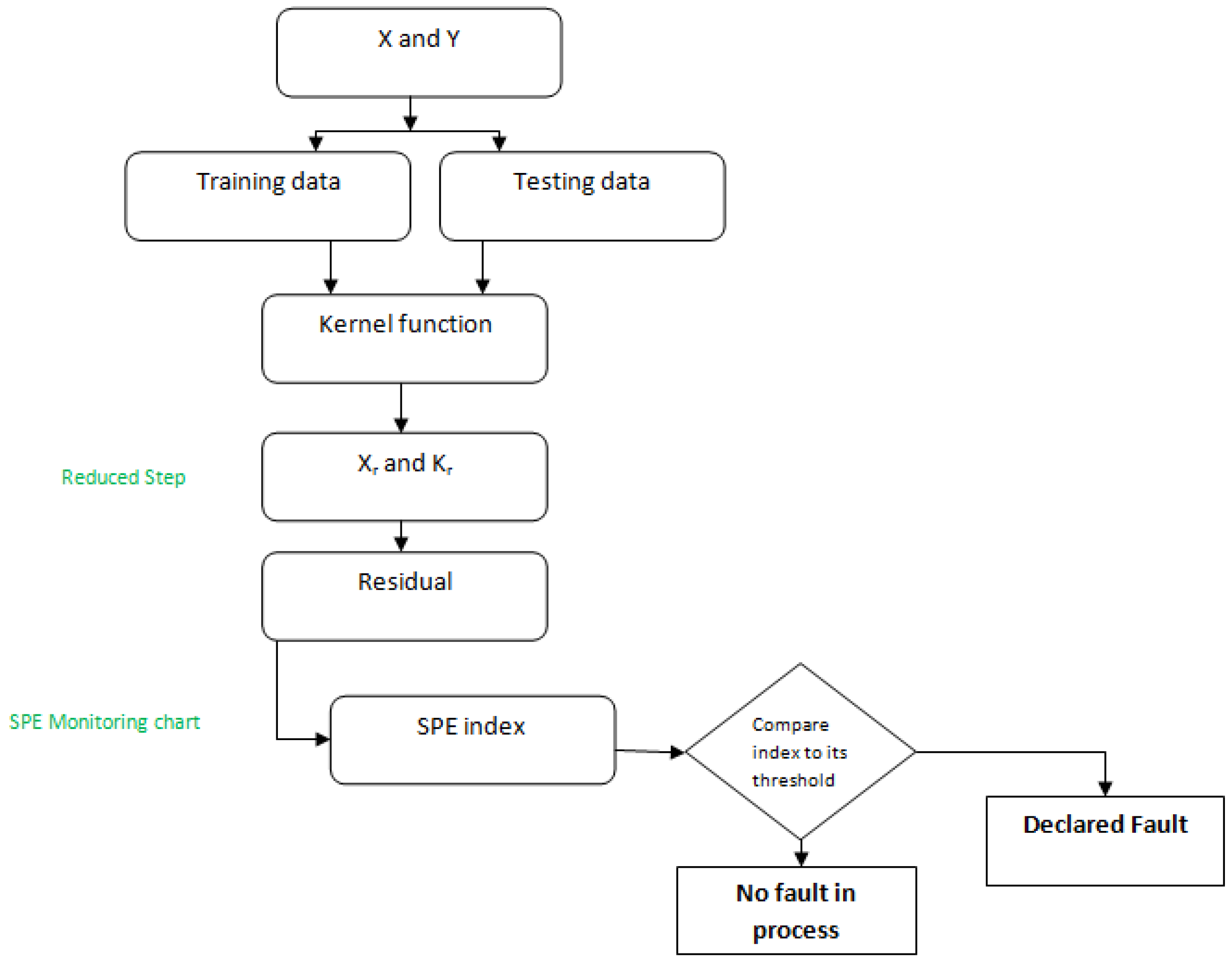
To sum up, the flowchart of the RKPLS and ORKPLS methods, are illustrated, respectively, in Figure 2 and Figure 3.

3. The Suggested Fault Isolation Methods

In this section, the focus is on the fault isolation phase and the identification of the faulty component. Several fault isolation methods have been proposed in the literature [15,38]. The monitored variables and parameters evolve within a measurement range considered normal operation; beyond that, it is a dysfunction that will have to be taken into consideration. However, it is necessary to identify the origin of the defect.
The principle of the isolation method, used in this part, is built upon the structured residuals. In effect, a set of residues is constructed in such a way such that each residual responds to specific faults while remaining insensitive to others.
This principle of isolation can be proposed for fault isolation in nonlinear dynamic systems based on RKPLS with a fixed model and ORKPLS method with an adaptive model.

3.1. Fault Isolation Based on RKPLS

The proposed partial RKPLS fault isolation method is a residue structuring approach based on the selection of groups of data points with following the removal of some variables or eliminated from the original data.
However, a partial RKPLS method is a RKPLS used as a reduced vector, where some data is missing. Thus, every defect triggers a particular response, using an appropriate combination of structured residues, called a fault signature. The fault signature is determined from the reduced RKPLS models using the SPE index and the detection thresholds.
The partial RKPLS based on the residue structuring generates structured indexes according to an appropriate matrix composed of 0s and 1s.
However, the main algorithmic steps of the partial RKPLS localization are presented as Algorithm 3:
Algorithm 3: Partial RKPLS localization algorithm
1-Construct a highly interpretable incidence matrix.
2-Implement RKPLS on the data matrix.
3-Determine a partial RKPLS model set, as well as each corresponding to a row of the theoretical signature matrix.
4-Select the control thresholds.
At each instant t
1-Calculate the S P E i indices for each of the partial RKPLS models.
2-Compare the S P E i indices to their appropriate confidence limits to determine the Experimental Signature (SE), as depicted in Equation (22).
S E i ( t ) = 0 i f S P E i ( t ) δ α , i 2 ( t ) 1 i f S P E i ( t ) > δ α , i 2 ( t )
3-Compare the experimental result with a column of the theoretical signature matrix to determine the location decision.
However, the theoretical signature matrix (incidence matrix) essentially contains “0” and “1”. In this case, the fault isolation is studied using a “strongly” localizable theoretical signature matrix.The matrix is defined as strongly localizable if it is impossible to obtain any column from another by substituting a “1” with a “0” The columns and the rows of an incidence matrix present the fault signatures and the structured indices, respectively.
Concerning the experimental signature matrix, “0” is obtained if the S P E i index is not sensitive to the fault and “1” if the S P E i index is sensitive to the fault.

3.2. Online Fault Isolation Based on ORKPLS

In this part, the same principle of partial RKPLS method is applied for the online method ORKPLS. Thus, the general concept is to use the ORKPLS method with a reduced data matrix that contains only the information-rich data. The residual, in this case, will only be sensitive to the defects linked to the variables determined in the reduced vector.
A strongly isolable incidence matrix was determined to generate the structured residuals for fault localization. This matrix presents the defects at the level of the columns and the residues appear in the rows.
As shown in the partial RKPLS method, when the residual is sensitive to the fault, the value of “1” is added; otherwise the value of “0” is added.
The principle of the online fault isolation proposed method is based on the generation of structured residuals acording to set of adaptive sub-models.
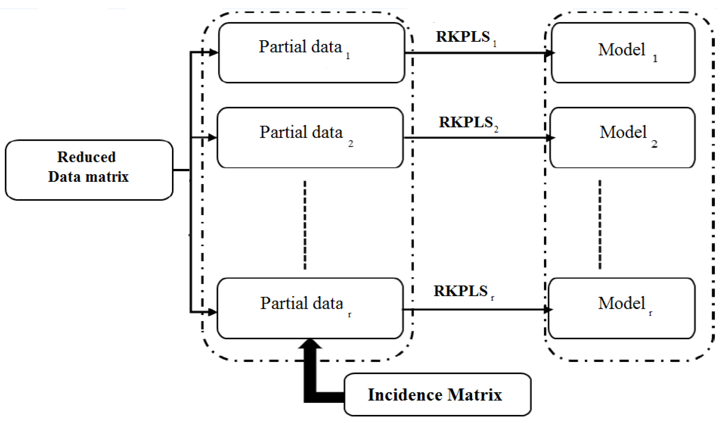
Thus, the following Figure 4 shows the procedure for the structured partial ORKPLS method.
So, the procedure for setting a structured partial ORKPLS is as illustrated:
  • Use the principle of the method reduced to the data matrices.
  • Determine an incidence matrix, in general, using strong isolation properties.
  • Determine a set of partial data using the ORKPLS method, each implementing a row of the incidence matrix.
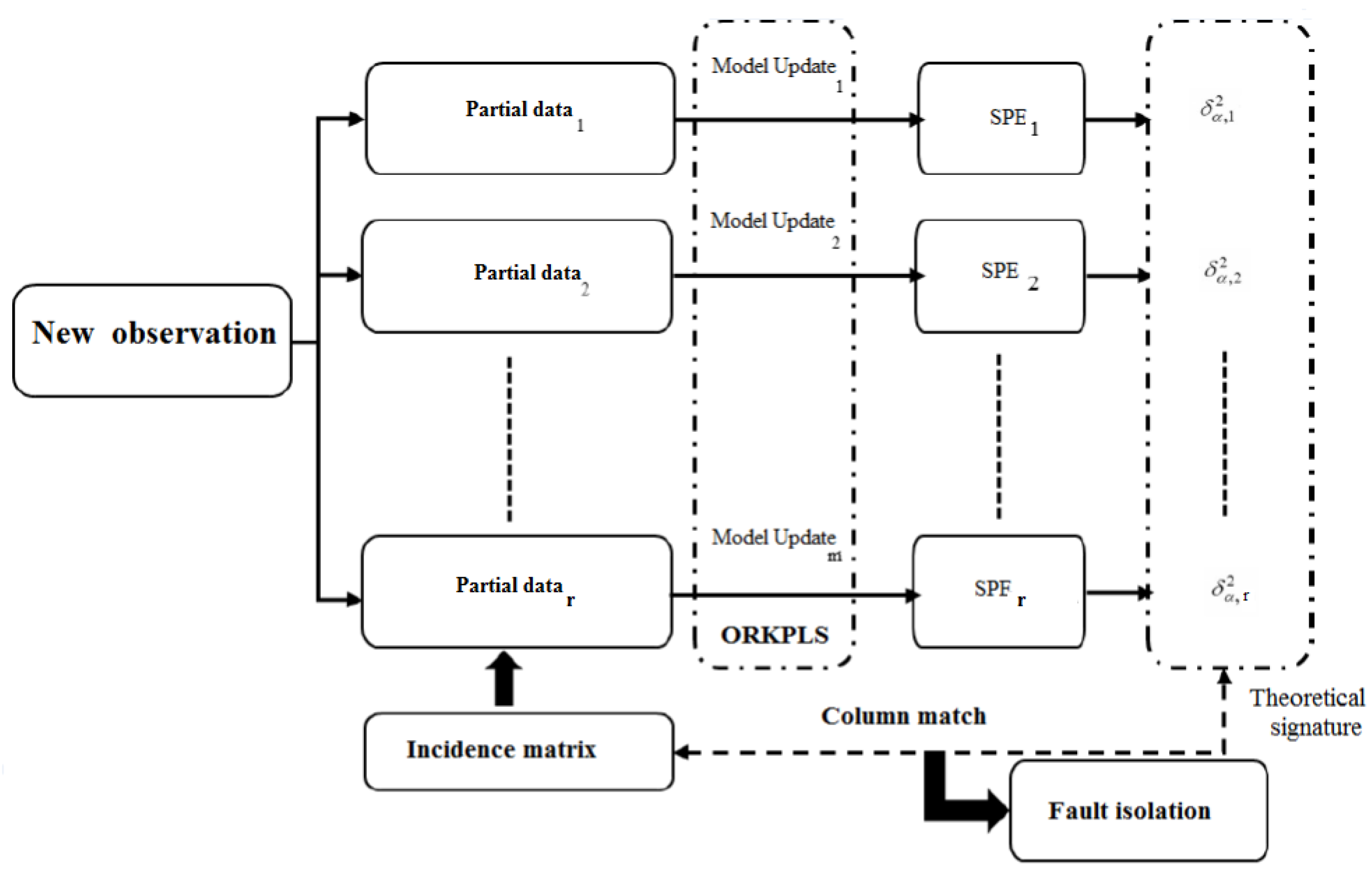
Afterwards, Figure 5 explains the principle of the isolation procedure using the structured partial ORKPLS. For the online fault isolation, the structured partial ORKPLS set obtained is used. The following steps describe the online isolation based on the partial ORKPLS method:
  • Calculate, for each partial model, the S P E i with i 1 , , r index and also its control limit S P E α , i , as depicted in Equation (20).
  • Make a comparison between the threshold and the control limit.
    S E i ( k ) = 1 i f S P E i ( k ) > S P E α , i ( k ) 0 i f S P E i ( k ) S P E α , i ( k )
    Then, S E i ( k ) = [ S E 1 ( k ) , , S E r ( k ) ] T is obtained.
  • For each moment, compare the difference between the fault code and the columns of the incidence matrix to get an idea about the localization decision.
The following Figure 5 summarizes all these steps.

4. Experimental Results

In this section, the suggested fault isolation method is applied to two systems to show the performance of the static and online methods.
The performance of the partial RKPLS method, which actually describes the static mode, is studied using the CSTR chemical system. Then, the online method, partial ORKPLS, is validated using the Air Quality Monitoring Network.

4.1. Case Study on CSTR Process

The CSTR chemical system is a non-linear process used for driving chemical reactions [39]. Generally, CSTR is a simple system to study. A simple validation of the proposed partial RKPLS method is conducted using the CSTR.

4.1.1. Process Description

The dynamic behavior describing a CSTR reactor is shown in the following equations:
d C A d t = F V ( C A 0 C A ) K 0 e E / R T C A d T A d t = F V ( T A 0 T A ) + ( Δ H ) k 0 ρ C p e E / R T C A q V ρ C p q = a F b + 1 F c + ( a F b 2 ρ c C p c ) ( T T c i n )
The variables of the CSTR process used to construct the data matrix are depicted in Table 1.
Then, the vector of measurements used to determine the X (data matrix) is illustrated in Equation (25).
X = [ F c F C A T ]
Indeed, for the CSTR, the temperature T and concentration C A are controlled and studied, based on built-in proportional controllers by manipulating, respectively, the inlet cooling water flow F c and the feed flow F.
One thousand observations were generated by changing the set points of the concentration C A and temperature T controllers in a stepwise manner. The training data is calculated on 500 samples, and the same is true for the testing data.

4.1.2. Simulation Results

To specify the performance of the proposed methods, the partial RKPLS method is first considered. In this part, the method is applied to 500 observations out of 1000 as training data X t r a i n i n g , with the remaining 500 used as testing data X t e s t i n g . The optimal kernel parameter is equal to 4.5 using the tabu search algorithm. Indeed, tabu search is an iterative metaheuristic described as local search in the broad sense. It consists of determining, in a flexible manner, a compromise between the quality of the solution and the computation time, as mentioned in [40].
The number of the reduced data is equal to 144.
Thus, fault localization is applied using the CSTR system to clearly illustrate the localization approach. The theoretical signature matrix developed for this application is presented in Table 2.
Following the structuring procedure using the partial RKPLS index, a set of four partial models was generated. Each partial RKPLS model is insensitive only to one variable.
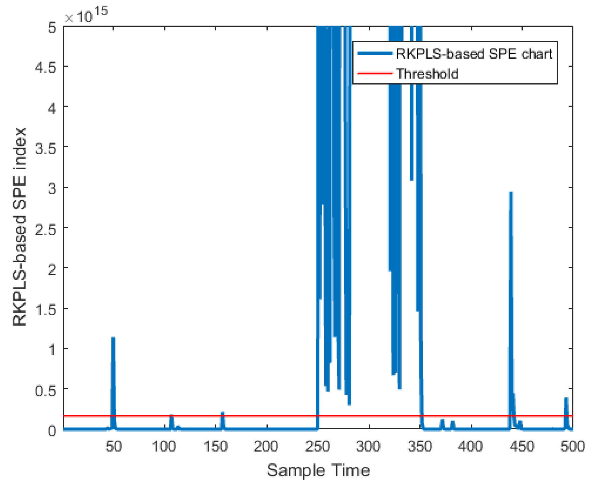
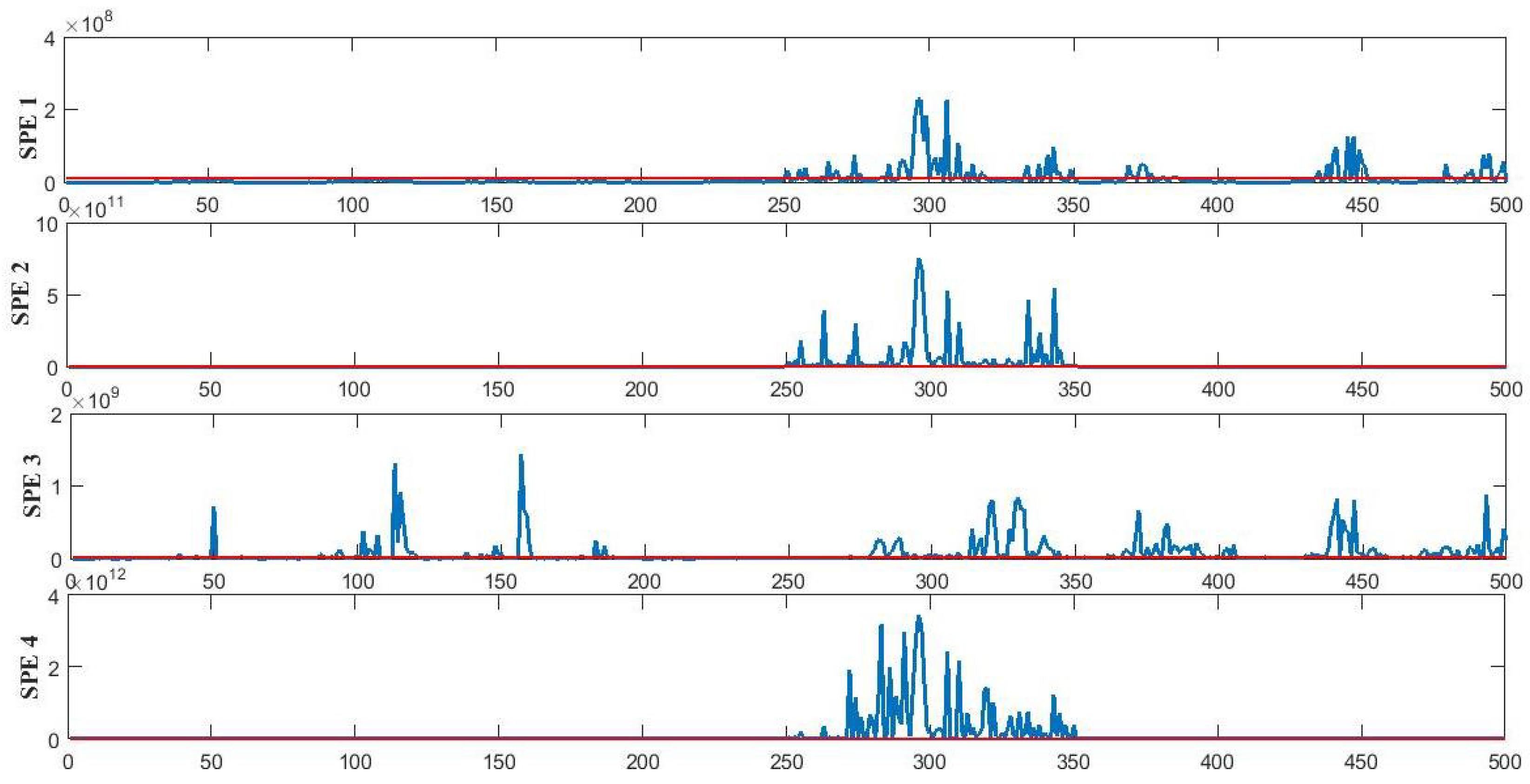
Subsequently, the focus is on the bias fault d 3 linked to the the concentration C A variable. The fault, in this case, is injected between observations 250 and 350. Figure 6 shows the d 3 fault detection results using the RKPLS detection method. After the fault has been presented and detected, it is necessary to locate it.
However, the suggested partial RKPLS method is applied. The fault isolation results using the proposed partial RKPLS are shown in Figure 7.
The evolution of different SPE indexes corresponding to the four partial RKPLS models in the case of the fault d 3 is shown in Figure 7. Indeed, the experimental signatures can be obtained as (1 1 0 1).
It can be noticed, in this case, that the experimental signature corresponds exactly to the third column of Table 2, which presents the theoretical incidence matrix. Finally, it is concluded that this variable is the faulty one.

4.2. Case Study on Air Quality Monitoring Network

In this part, the suggested fault isolation strategy is considered to diagnosis of an (AIRLOR) air quality monitoring network. In the following subsections, the AIRLOR network and the experimental results of the partial ORKPLS method are discussed.

4.2.1. Process Description

The AIRLOR is an air quality surveillance network located in Lorraine, France [41]. The AIRLOR essentially contains twenty stations placed in
  • Rural sites;
  • Peri-urban sites;
  • Urban sites.
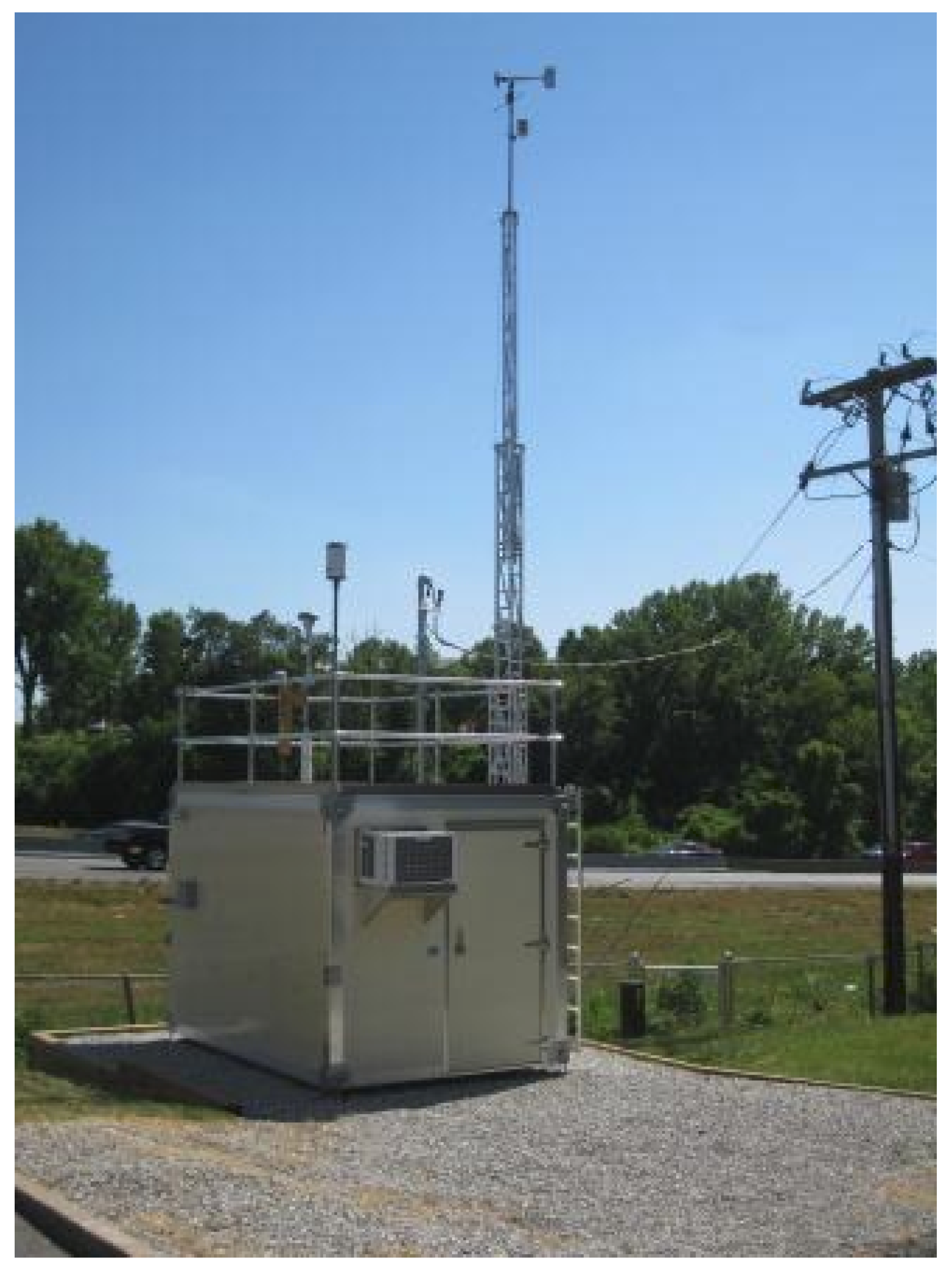
Each station is dedicated to determining certain air pollutants. Thus, with these stations, the concentration of nitrogen oxides (NO and NO2), carbon monoxide (CO), ozone (O3) and sulfur dioxide (SO2) can be controlled. Moreover, the AIRLOR has stations which for determining meteorological parameters. Nitrogen oxides (NO and NO2) are considered the primary pollutants, which are more localized due to their emissions sources. Then, ozone O3 is considered as a secondary pollutant and the spatial distribution of the greatest values is mostly homogeneous at a local scale. To guarantee human health, the study of tropospheric ozone has become very important in the last decade, making it one of the most studied topics. Figure 8 presents the air quality monitoring station.
Following these stations, the concentration measurements are carried out continuously all year round, 24 h a day. The different stations are linked together by a central computer via a telephone line. All data is transferred every day. All data is processed and validated, first manually and then statistically, before being grouped into a database and transmitted to the media [42].
The general principle is to detect and isolate sensor faults, which consists of determining ozone (O3) and nitrogen oxide (NO and NO2) concentrations.
In this paper, six of the neighboring measurement stations are presented. Nevertheless, it considered 18 variables of the x ( k ) input matrix made of nitrogen oxides, namely NO2 and NO, and ozone O3, named z 1 , z 2 , , z 18 , respectively, collected from each station.
x ( k ) = z 1 ( k ) z 2 ( k ) z 3 ( k ) S t a t i o n 1 z 10 ( k ) z 11 ( k ) z 12 ( k ) S t a t i o n 3 z 16 ( k ) z 17 ( k ) z 18 ( k ) S t a t i o n 6 T
The objective in this paper is to properly locate and isolate the fault using the suggested partial ORKPLS.

4.2.2. Simulation Results

To study the fault isolation performance for the partial ORKPLS method, 500 observation are used, out of 1080, as training data X t r a i n i n g , also the same number was employed for the testing data X t e s t i n g . A total of 224 observations were retained after data reduction. In this paper, the optimal kernel parameter has been determined using the algorithm of tabu search. The kernel parameter of the AIRLOR model achieved its optimal value at 25.37. The SPE setting is used to indicate the appearance of the defect with a confidence limit equal to 95%.
The incidence matrix employed in the AIRLOR simulations is presented in Table 3. The table allows for easy localization of relevant information. Table 3 displays 18 partial models, where each model is unaffected by two variables. Each fault d i , i = 1 , , 18 is sensitive to a variable of the data matrix x(k).
To demonstrate the effectiveness of the ORKPLS method for fault detection and isolation, a bias faul d 11 was applied to variable z 11 over the observation range from 200 to 400. Indeed, the fault amplitude represents 30 % of the total variation range of the variable.
Figure 9 present fault detection using the ORKPLS method. After the fault has been presented and detected, it should be located.
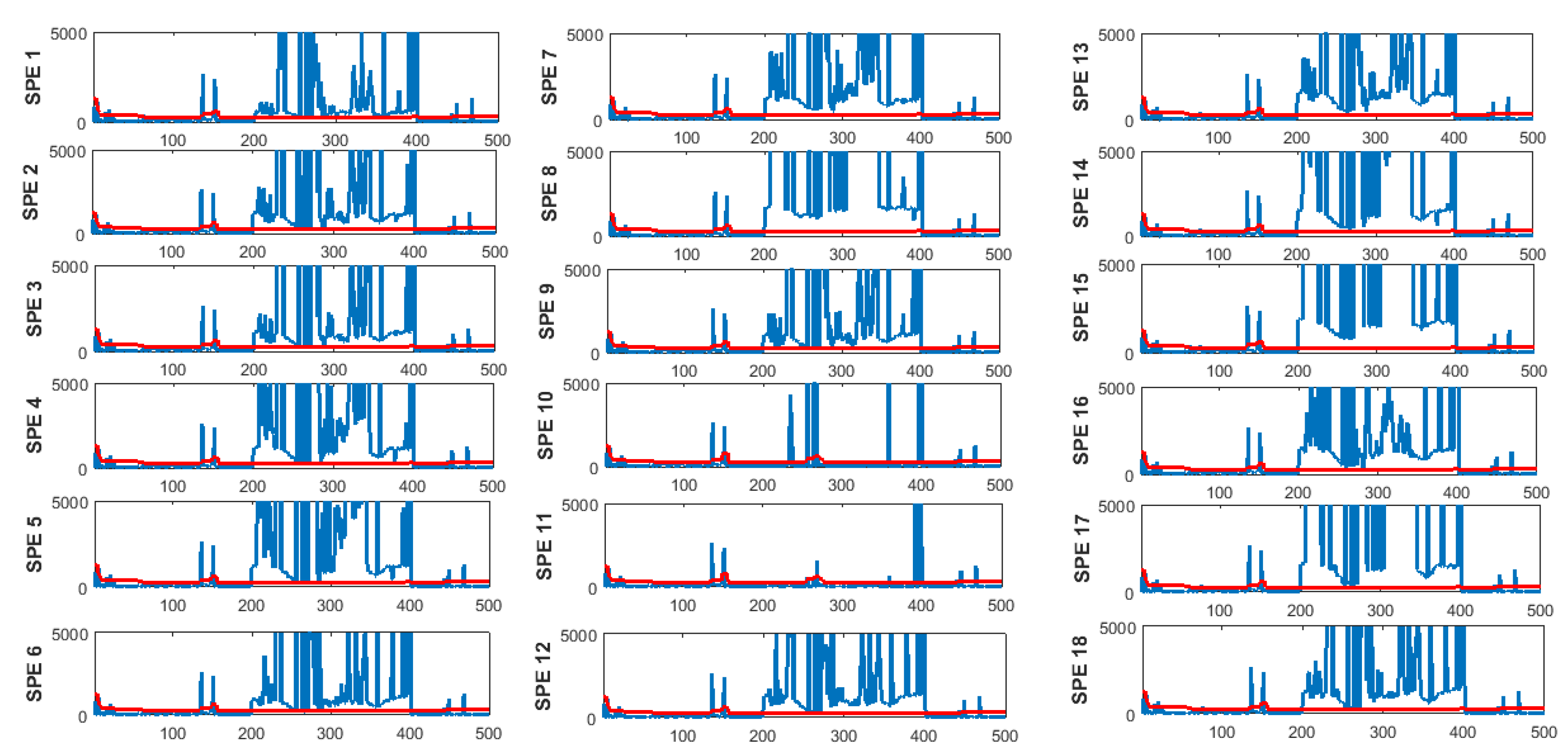
The suggested partial ORKPLS approach is applied, and fault isolation results using the suggested partial ORKPLS are displayed in Figure 10. In this figure, the blue lines represent ORKPLS based in SPE index and the red lines represent the threshold.
For each curve shown in Figure 10, an SPE index exceeding its control limit is assigned a value of “1” in the corresponding fault code, while an SPE index below its control limit is assigned a value of “0”. Each structured residual is designed to be sensitive to a specific subset of faults. Figure 10 illustrates the evolution of the SPE indices for the 18 partial ORKPLS models in the presence of fault d 11 . The experimental signatures in this case, can be seen in Figure 10, as (1 1 1 1 1 1 1 1 1 0 0 1 1 1 1 1 1 1).
Therefore, the simulation results from Figure 10 corresponded exactly to the 11th column of the incidence matrix. More precisely, it can be noticed that the experimental signature is identical to the 11th column of the Table 3, which presents the theoretical incidence matrix for the AIRLOR system. Finally, it is concluded that the variable z 11 is the faulty one.
It can be concluded that, for the fault isolation task, the suggested approachs (partial RKPLS and partial ORKPLS) have properly located the injected defects.
According the Table 4, the reduced method significantly optimizes the computation time required for fault detection in nonlinear systems while preserving the data structure in the feature space. In this case, an approach for online fault detection and isolation is presented. It proposes extending the partial PLS-based localization method by leveraging a dimensionality reduction in the feature-space kernel matrix.
The method proposed in this paper is limited by sensitivity to noise and reduced interpretability of fault sources. The developed techniques are planned to be extended to handle data uncertainty using interval modeling. Indeed, interval-based approaches can be employed to improve fault detection accuracy, robustness to noise, and interpretability. This will enable the development of a new interval-based online monitoring strategy for uncertain industrial processes.
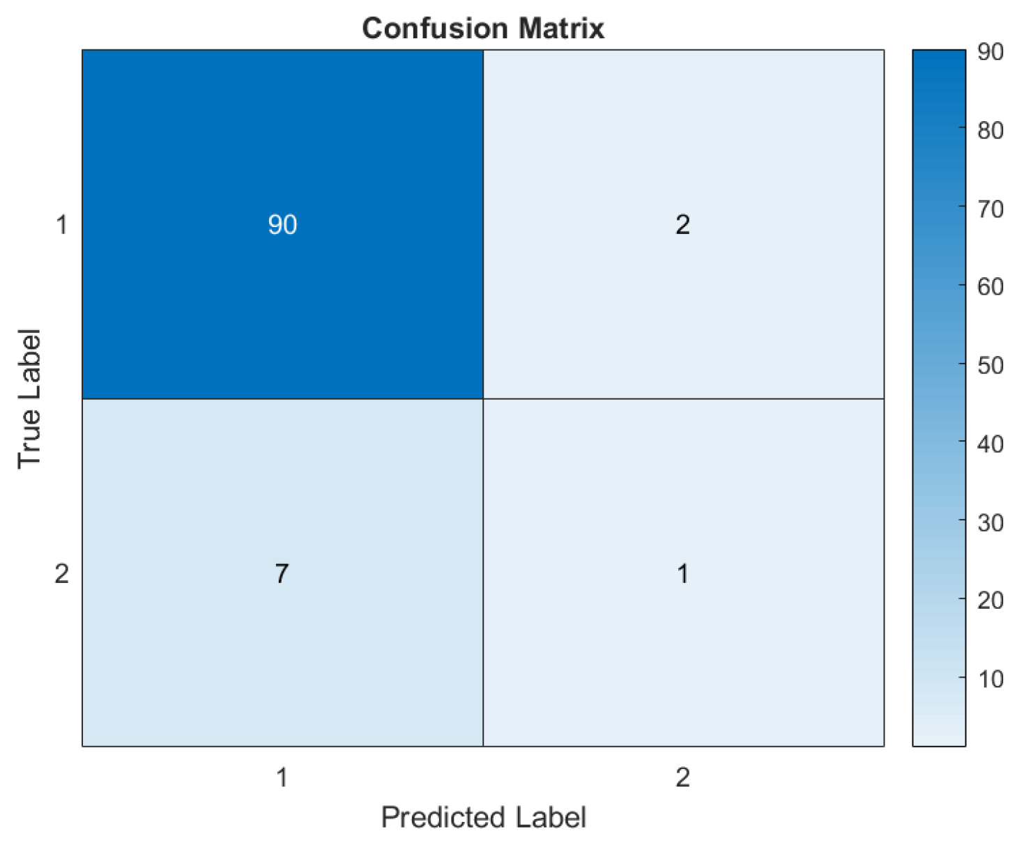
Figure 11 shows a confusion matrix for the KNN (K-Nearest Neighbors) classification model. To provide a comprehensive evaluation of classification performance, this confusion matrix consists of starting from the test subset of the database, to evaluate the performance of the model in terms of fault detection in offline mode. Each matrix cell shows the number of predictions for a specific class; diagonal entries correspond to correct classifications, while off-diagonal entries indicate misclassifications.
All the analysis of the evaluation measures are grouped in Table 5.

5. Conclusions

In this paper, a new online and reduced data-driven fault isolation method has been suggested for nonlinear system security.
The main contributions of this work are grouped into two main points:
  • The RKPLS method uses only useful and relevant data for fault detection. Thus, the proposed partial RKPLS method is a useful approach for fault isolation.
  • The reference model for the online method is updated if a new observation becomes available and satisfies the independence condition between variables in the feature space.
Thus, the partial ORKPLS method proposed in this paper uses structured residuals based on symmetry to compose a fault isolation scheme from a properly designed incidence matrix. The objective of this paper is to achieve good fault isolation using a reduced and online method. For fault isolation, the partial RKPLS and partial ORKPLS methods perform well with the CSTR and AIRLOR processes.
To conclude, this study demonstrates that detecting and locating faults in real time is an effective way to secure nonlinear systems. By exploiting the underlying symmetry in process data, the proposed online reduced model provides robust monitoring, ensuring reliable fault localization and preventing sudden risks. This gives us the possibility of controlling the state of the system and locating the faults to avoid any dangers and risks.
The principal limitations of fault isolation based on partial KPLS are, in general, sensitivity to kernel choice, limited fault observability, computational complexity and data dependency. In this paper, the proposed approach present:
  • Kernel Optimization: Select optimal kernel parameters using the Tabu search algorithm to improve the classical KPLS model.
  • Reference Model Construction: Extract the most relevant observations to reduce computation time in feature space projections.
  • Online Model Updating: Update the reference model when a new accurate observation satisfies independence conditions between variables.
  • Online Fault Isolation: Develop ORKPLS-based approaches for real-time fault isolation.
As for future work, the development of online detection and isolation methods for uncertain industrial processes is of interest. Furthermore, the ORKPLS method is intended to be extended to study data uncertainty using several approaches, such as interval modeling.

Author Contributions

Conceptualization, M.S.; Formal analysis, O.T.; methodology, M.S. and W.G.; Project administration, O.T.; software, M.S.; validation, O.T. and K.Z.; writing-original draft preparation, M.S. and O.T.; writing-review and editing, M.S., K.Z. and W.G.; visualization, M.S.; supervision, O.T., K.Z. and W.G.; project administration, O.T. All authors have read and agreed to the published version of the manuscript.

Funding

The authors received no specific funding for this study.

Data Availability Statement

Data is contained within the article.

Acknowledgments

The authors thank Khawla Ben Abdellafou for her valuable comments on the early version of this manuscript.

Conflicts of Interest

The authors declare no conflicts of interest.

References

  1. Iulian, L.; Mihaiela, L. Machine Learning Techniques for Multi-Fault Analysis and Detection on a Rotating Test Rig Using Vibration Signal. Symmetry 2023, 15, 86. [Google Scholar]
  2. Seongjun, K.; Jihye, H.; Sang, K.; Sang, C.; Ohbyung, K. Leveraging Quantum Machine Learning to Address Class Imbalance: A Novel Approach for Enhanced Predictive Accuracy. Symmetry 2025, 17, 186. [Google Scholar] [CrossRef]
  3. Abid, A.; Khan, M.; Iqbal, J. A review on fault detection and diagnosis techniques: Basics and beyond. Artif. Intell. Rev. 2021, 54, 3639–3664. [Google Scholar] [CrossRef]
  4. Han, S.; Hua, Y.; Lin, Y.; Yao, L.; Wang, Z.; Zheng, Z.; Yang, J.; Zhao, C.; Zheng, C.; Gao, X. Fault diagnosis of regenerative thermal oxidizer system via dynamic uncertain causality graph integrated with early anomaly detection. Process Saf. Environ. Prot. 2023, 179, 724–734. [Google Scholar] [CrossRef]
  5. Muratbakeev, E.; Kozhubaev, Y.; Novak, D.; Ershov, R.; Wei, Z. Monitoring and Diagnostics of Mining Electromechanical Equipment Based on Machine Learning. Symmetry 2025, 17, 1548. [Google Scholar] [CrossRef]
  6. Taha, U.; Suhail, H.; Ahsen, U.; Ahmet, O.; Muhammad, R.; Daisuke, M. Machine Learning-Based Intrusion Detection for Achieving Cybersecurity in Smart Grids Using IEC 61850 GOOSE Messages. Symmetry 2021, 13, 826. [Google Scholar] [CrossRef]
  7. Kim, L.; Lee, J.D.; Lee, S.; Bang, H. Fault Detection for Re-initialization of Online Gaussian Process Regression Using Kernel Linear Independence Test. Int. J. Control Autom. Syst. 2024, 22, 3386–3395. [Google Scholar]
  8. Sun, Z.; Wang, X.; Han, T.; Wang, L.; Zhu, Z.; Huang, H.; Ding, J.; Wu, Z. Pipeline deformation prediction based on multi-source monitoring information and novel data-driven model. Eng. Struct. 2025, 337, 120461. [Google Scholar] [CrossRef]
  9. Sun, Z.; Wang, X.; Han, T.; Huang, H.; Huang, X.; Wang, L.; Wu, Z. Pipeline deformation monitoring based on long-gauge FBG sensing system: Missing data recovery and deformation calculation. J. Civ. Struct. Health Monit. 2025, 15, 2433–2453. [Google Scholar]
  10. Mohammed, K.; Abdelmalek, K.; Mohamed, H.; Abderazak, B.; Majdi, M. Data size reduction approach for nonlinear process monitoring refinement using Kernel PCA technique. Expert Syst. Appl. 2025, 274, 126975. [Google Scholar] [CrossRef]
  11. Kim, H.; Chang, H.; Shim, H. Evaluating MR-GPR and MR-NN: An Exploration of Data-driven Control Methods for Nonlinear Systems. Int. J. Control Autom. Syst. 2024, 22, 2934–2941. [Google Scholar] [CrossRef]
  12. Taqvi, S.A.; Zabiri, H.; Tufa, L.; Uddin, F.; Fatima, S.A.; Maulud, A.S. A review on data-driven learning approaches for fault detection and diagnosis in chemical processes. ChemBioEng Rev. 2021, 8, 239–259. [Google Scholar] [CrossRef]
  13. Ziyao, S.; Han, Z.; Jianfang, J. Data-Driven State of Health Interval Prediction for Lithium-Ion Batteries. Electronics 2024, 13, 3991. [Google Scholar]
  14. Hasnen, S.; Shahid, M.; Zabiri, H.; Taqvi, S. Semi-supervised adaptive PLS soft-sensor with PCA-based drift correction method for online valuation of NOx emission in industrial water-tube boiler. Process Saf. Environ. Prot. 2023, 172, 787–801. [Google Scholar] [CrossRef]
  15. Zhang, Y.; Ma, C. Fault diagnosis of nonlinear processes using multiscale KPCA and multiscale KPLS. Chem. Eng. Sci. 2011, 66, 64–72. [Google Scholar] [CrossRef]
  16. Silalahi, D.; Midi, H.; Arasan, J.; Mustafa, M.; Caliman, J. Kernel partial least square regression with high resistance to multiple outliers and bad leverage points on near-infrared spectral data analysis. Symmetry 2021, 13, 547. [Google Scholar] [CrossRef]
  17. Bennett, K.; Embrechts, M. An optimization perspective on kernel partial least squares regression. Nato Sci. Ser. Sub Ser. III Comput. Syst. Sci. 2003, 190, 227–250. [Google Scholar]
  18. Hu, W.; Wang, Y.; Li, Y.; Wan, X.; Gopaluni, R. A multi-feature-based fault diagnosis method based on the weighted timeliness broad learning system. Process Saf. Environ. Prot. 2024, 183, 231–243. [Google Scholar] [CrossRef]
  19. Tidriri, K.; Chatti, N.; Verron, S.; Tiplica, T. Bridging data-driven and model-based approaches for process fault diagnosis and health monitoring: A review of researches and future challenges. Annu. Rev. Control 2016, 42, 63–81. [Google Scholar] [CrossRef]
  20. Ge, Z. Review on data-driven modeling and monitoring for plant-wide industrial processes. Chemom. Intell. Lab. Syst. 2017, 171, 16–25. [Google Scholar] [CrossRef]
  21. Said, M.; Abdellafou, K.; Taouali, O.; Harkat, F. A new monitoring scheme of an air quality network based on the kernel method. Int. J. Adv. Manuf. Technol. 2019, 103, 153–163. [Google Scholar] [CrossRef]
  22. Lahdhiri, H.; Taouali, O. Reduced Rank KPCA based on GLRT chart for sensor fault detection in nonlinear chemical process. Measurement 2021, 169, 108342. [Google Scholar] [CrossRef]
  23. Mok, H.; Chan, C. Online fault detection and isolation of nonlinear systems based on neurofuzzy networks. Eng. Appl. Artif. Intell. 2008, 21, 171–181. [Google Scholar] [CrossRef]
  24. Chan, C.; Cheung, K.; Wang, Y.; Chan, W. Online fault detection and isolation of nonlinear systems. In Proceedings of the 1999 American Control Conference (Cat. No. 99CH36251), San Diego, CA, USA, 2–4 June 1999; Volume 6, pp. 3980–3984. [Google Scholar]
  25. Ellefsen, A.; Han, P.; Cheng, X.; Holmeset, F.; Vilmar, A.; Zhang, H. Online fault detection in autonomous ferries: Using fault-type independent spectral anomaly detection. IEEE Trans. Instrum. Meas. 2020, 69, 8216–8225. [Google Scholar] [CrossRef]
  26. Wahbe, R.; Lucco, S.; Anderson, T.; Graham, S. Efficient software-based fault isolation. In Proceedings of the Fourteenth ACM Symposium on Operating Systems Principles, Asheville, NC, USA, 5–8 December 1993; pp. 203–216. [Google Scholar]
  27. Laib, A.; Terriche, Y.; Melit, M.; Su, C.; Mutarraf, M.; Bouchekara, H.R.; Guerrero, J.M.; Boudjefdjouf, H. Enhanced artificial intelligence technique for soft fault localization and identification in complex aircraft microgrids. Eng. Appl. Artif. Intell. 2024, 127, 107289. [Google Scholar] [CrossRef]
  28. Yeu, T.; Kim, H.; Kawaji, S. Fault detection, isolation and reconstruction for descriptor systems. Asian J. Control 2005, 7, 356–367. [Google Scholar] [CrossRef]
  29. Zhang, Y.; Zhou, H.; Qin, S.; Chai, T. Decentralized fault diagnosis of large-scale processes using multiblock kernel partial least squares. IEEE Trans. Ind. Inform. 2009, 6, 3–10. [Google Scholar] [CrossRef]
  30. Jia, Q.; Zhang, Y. Quality-related fault detection approach based on dynamic kernel partial least squares. Chem. Eng. Res. Des. 2016, 106, 242–252. [Google Scholar] [CrossRef]
  31. Rosipal, R.; Trejo, L.J. Kernel partial least squares regression in reproducing kernel hilbert space. J. Mach. Learn. Res. 2001, 2, 97–123. [Google Scholar]
  32. Zhang, Y.; Hu, Z. Multivariate process monitoring and analysis based on multi-scale KPLS. Chem. Eng. Res. Des. 2011, 89, 2667–2678. [Google Scholar] [CrossRef]
  33. Lindgren, F.; Geladi, P.; Wold, S. The kernel algorithm for PLS. J. Chemom. 1993, 7, 45–59. [Google Scholar] [CrossRef]
  34. Kim, K.; Lee, J.M.; Lee, I.B. A novel multivariate regression approach based on kernel partial least squares with orthogonal signal correction. Chemom. Intell. Lab. Syst. 2005, 79, 22–30. [Google Scholar] [CrossRef]
  35. Said, M.; Abdellafou, K.; Taouali, O. Machine learning technique for data-driven fault detection of nonlinear processes. J. Intell. Manuf. 2020, 31, 865–884. [Google Scholar] [CrossRef]
  36. Dunia, R.; Qin, S.J. Joint diagnosis of process and sensor faults using principal component analysis. Control Eng. Pract. 2005, 6, 457–469. [Google Scholar] [CrossRef]
  37. Jackson, J.E.; Mudholkar, G.S. Control procedures for residuals associated with principal component analysis. Technometrics 1979, 21, 341–349. [Google Scholar] [CrossRef]
  38. Navi, M.; Meskin, N.; Davoodi, M. Sensor fault detection and isolation of an industrial gas turbine using partial adaptive KPCA. J. Process Control 2018, 64, 37–48. [Google Scholar] [CrossRef]
  39. Zhang, X.; Deng, X.; Cao, Y.; Xiao, L. Nonlinear Predictable Feature Learning with Explanatory Reasoning for Complicated Industrial System Fault Diagnosis. Knowl.-Based Syst. 2024, 286, 111404. [Google Scholar] [CrossRef]
  40. Ben Abdellafou, K.; Hadda, H.; Korbaa, W. An improved tabu search meta-heuristic approach for solving scheduling problem with non-availability constraints. Arab. J. Sci. Eng. 2019, 44, 3369–3379. [Google Scholar] [CrossRef]
  41. Harkat, M.; Mourot, G.; Ragot, J. An improved PCA scheme for sensor FDI: Application to an air quality monitoring network. J. Process Control 2006, 16, 625–634. [Google Scholar] [CrossRef]
  42. Harkat, M.; Mourot, G.; Ragot, J. Sensor failure detection of air quality monitoring network. IFAC Proc. Vol. 2006, 33, 529–534. [Google Scholar] [CrossRef]
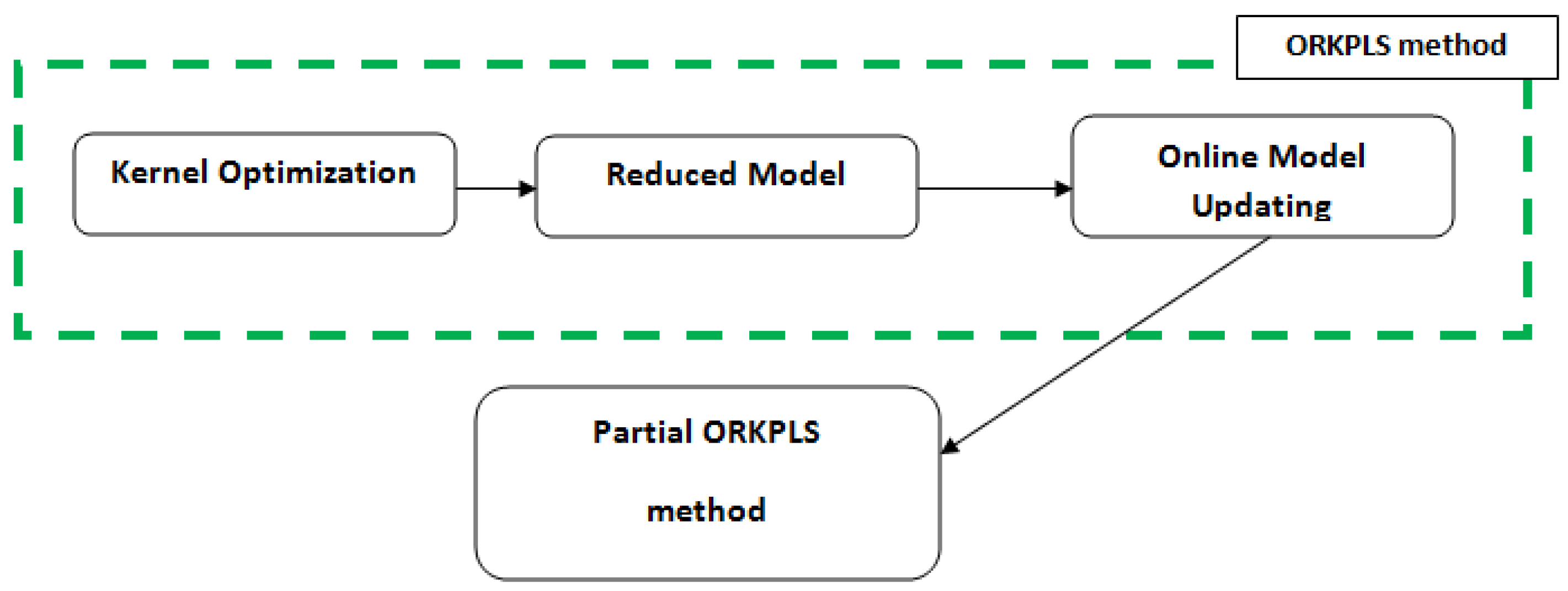
Figure 1. The main contributions of this study.
Symmetry 17 01863 g001
Figure 2. Flowchart of RKPLS-based SPE chart.
Symmetry 17 01863 g002
Figure 3. Flowchart of ORKPLS-based SPE chart.
Symmetry 17 01863 g003
Figure 4. Procedure of structured partial ORKPLS method.
Symmetry 17 01863 g004
Figure 5. Procedure of localization using partial ORKPLS method.
Symmetry 17 01863 g005
Figure 6. Evolution of the SPE index with fault d 3 using RKPLS.
Symmetry 17 01863 g006
Figure 7. Evolution of different SPEs corresponding to the 4 partial RKPLS models in the case of the fault d 3 .
Symmetry 17 01863 g007
Figure 8. The monitoring station for air pollutants (air quality).
Symmetry 17 01863 g008
Figure 9. Variation of the SPE index during the fault scenario d 11 using ORKPLS.
Symmetry 17 01863 g009
Figure 10. Evolution of different SPEs associated with the 18 partial ORKPLS models in the case of fault d 11 . In this figure, the blue lines represent ORKPLS based in SPE index and the red lines represent the threshold.
Symmetry 17 01863 g010
Figure 11. Confusion matrices for the KNN model.
Symmetry 17 01863 g011
Table 1. Measurement variables for the CSTR chemical reactor.
VariablesDescriptionValue
C A The flow concentration of the inlet A1 (mol/L)
k 0 The reaction rate constant4.11  ×   10 13 (L/min·mol)
EActivation energy76,534 (J/mol)
T A 0 The temperature of the inlet flow into the reactor350 (K)
T c i n Coolant inlet temperature350 (K)
Δ H The heat of reaction596,619 (J/mol)
TThe temperature of the inlet stream-
FFlow in and out of the reactor-
VThe volume of the reactor100 (L)
RReal gas constant8.31451 (J/mol·K)
ρ The density of the reactor contents and all streams1000 (J/L)
C p Capacity of reactor contents and all streams4.25 (J/g·K)
Table 2. The incidence matrix of CSTR system.
d 1 d 2 d 3 d 4
r 1 0111
r 2 1011
r 3 1101
r 4 1110
Table 3. The incidence matrix of AIRLOR system.
d 1 d 2 d 3 d 4 d 5 d 6 d 7 d 8 d 9 d 10 d 11 d 12 d 13 d 14 d 15 d 16 d 17 d 18
r 1 001111111111111111
r 2 100111111111111111
r 3 110011111111111111
r 4 111001111111111111
r 5 111100111111111111
r 6 111110011111111111
r 7 111111001111111111
r 8 111111100111111111
r 9 111111110011111111
r 10 111111111001111111
r 11 111111111100111111
r 12 111111111110011111
r 13 111111111111001111
r 14 111111111111100111
r 15 111111111111110011
r 16 111111111111111001
r 17 111111111111111100
r 18 011111111111111110
Table 4. The computation time for the algorithms KPLS, RKPLS and ORKPLS.
Computation Time (s)AIRLORCSTR
KPLS1.1040.87
RKPLS0.980.69
ORKPLS0.8710.44
Table 5. Fault detection evaluation metrics (offline mode).
Confusion Matrix
FP FN TP TN Accuracy Precision Sensitivity Total Events
Modelo KNN9072191%92.86%97.83%100
Disclaimer/Publisher’s Note: The statements, opinions and data contained in all publications are solely those of the individual author(s) and contributor(s) and not of MDPI and/or the editor(s). MDPI and/or the editor(s) disclaim responsibility for any injury to people or property resulting from any ideas, methods, instructions or products referred to in the content.