Arc Fault Location for Photovoltaic Distribution Cables Based on Time Reversal

Abstract

The direct current (DC) cable serves as the link for energy output in photovoltaic (PV) systems. Its degradation can cause arcs, which easily lead to fire accidents. Locating arc faults, however, is challenging. To cope with it, this paper proposes an arc location method based on time reversal. The method has been tried to locate system fault. However, its application in the arc fault location of photovoltaic systems is seldom discussed and needs further research. For this purpose, the voltage waveforms of an arc fault collected at one of the cable ends is reversed. This transformation derives a symmetrical arc fault signal. Afterwards, the reversed signal is injected back into the cable to trace the fault location, which is a symmetrical process of the arc fault signal travelling from its origin to the detection point. Utilizing the energy-focusing characteristics of time reversal, the position with the highest energy in the derived waveform corresponds to the actual fault location. To verify the proposed method, a DC arc fault test is performed to obtain the wave characteristics. The Paukert arc model is chosen based on the tested result. A PV system containing a DC cable with an arc fault is simulated with Simulink with the affecting factors, i.e., grounded resistance, cable length, fault location and sampling frequency. The simulated results demonstrate that the localization error is within 5% in the worst case.

1. Introduction

An energy system is transformed into a more environment friendly one under the guidance of low carbon emissions. The number of photovoltaic (PV) systems is growing rapidly worldwide, and it is expected that the installed capacity of solar PVs can meet more than 30% of power demand by 2050 [1]. DC busbar cables, as the backbone lines for energy transmission in PV systems, are prone to arc faults and fire accidents under the influence of prolonged exposure to harsh environments [2].

When the arc occurs, it is vital to precisely locate the arc faults. During an arc fault, the electrical parameters, such as voltage, throughout the circuit will change [3]. These electrical parameters contain time/location information, which can be used to locate the arc fault. Compared with offline locations, an online location is preferred since it can improve the maintenance efficiency significantly. The conventional online positioning methods for power cable arc faults can be categorized into impedance-based methods and traveling wave-based methods. For the impedance-based approach, the voltage and current with the fundamental component are utilized to calculate the impedance during the arc to determine its location. This method is widely applied due to its low-cost advantage. However, the location accuracy is greatly affected by the fault type and circuit information [4]. The working principle of travelling wave technology is that when an arc fault occurs in the cable, electromagnetic waves propagating along the cable will be generated. By measuring the time delay of the electromagnetic wave in the line, the fault point is located. However, the need for communication and time synchronization between devices at different detection points makes implementing them costly. In addition, the accuracy of the method is affected by the distortion of the fault signal as it propagates along the line as well as by electromagnetic interference (EMI) [5].

The theory of electromagnetic time reversal (EMTR) was first proposed in 1957 [6]. It is applied in industries such as acoustics and electromagnetic waves [7,8]. EMTR was introduced to fault location in 2012 [9]. Since then, it has been studied for the localization of electromagnetic interference sources in power systems [10,11]. The wave generated by an arc propagates along the cable. The time-reversed measured waves are injected back into the cable where it is extracted, which would converge in a phase at the initial fault location. Previously, it was studied for various scenarios. Reference [12] used this method to locate lightning strikes. Reference [13] discussed the norm criteria for fault location with time reversal utilizing signals from both ends of the transmission line. Reference [14] extended the time reversal method to partial discharge location. Reference [15] analyzed the fault location capability of EMTR in mismatched media. Pilot projects and field experiments have been tested based on this method [11,16]. Studies also tried to improve the efficiency of this method by utilizing the concept of transient convolution [17]. Though numerous research has been conducted for the fault positioning based on time reversal, its application in arc fault location in photovoltaic systems is seldom discussed and needs further research. Specifically, the arc fault characteristics in PV distribution cables is different from other types of faults, which may pose a challenge for the time reversal method. A previous study has shown the great potential of using time reversal technology in various faults’ location. Therefore, this paper proposes a method based on the principle of time reversal for the localization of cable arc faults in photovoltaic systems. The feasibility is discussed via a dedicated model embedded with an arc fault signal extracted from the experiment. Additionally, the affecting factors of the method on arc fault location in PV cables are analyzed in depth, namely grounded resistance, cable length, fault location and sampling frequency.

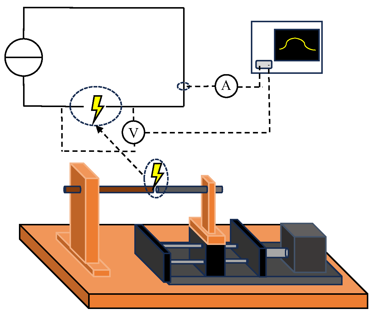
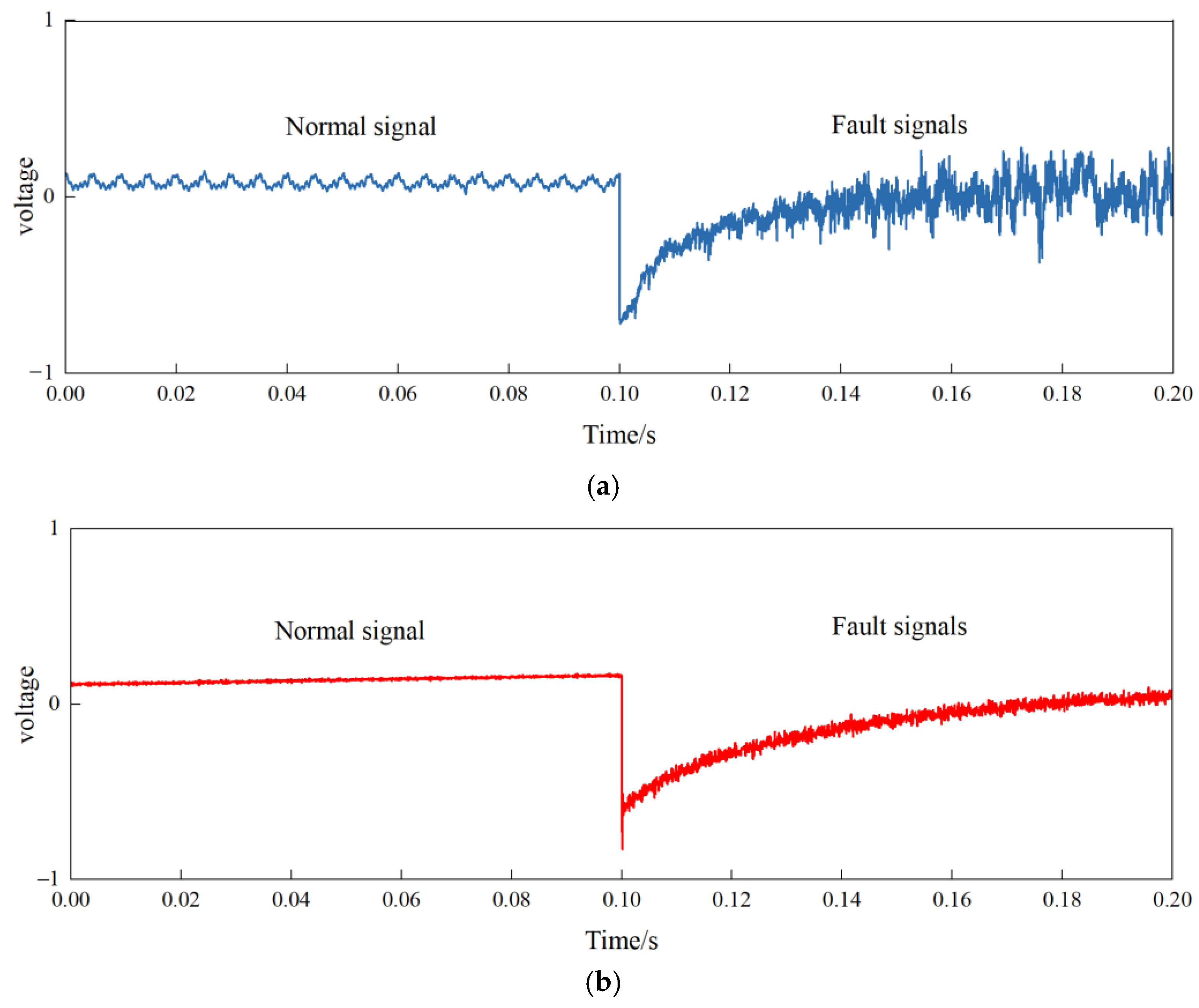
In this paper, a DC arc test platform is established to obtain the typical electric signal. The Paukert model is then applied for the arc simulation. The arc fault propagation and the basic principle of the EMTR technique are then discussed. The time reversal process of the detected signal is elaborated in detail. An approach to apply the time reversal method to locate faults in PV systems is proposed with only one observation point. Then, the arc fault localization of the PV system is simulated by Simulink 2021a to verify the effectiveness of the proposed method, where different affecting factors are discussed.

2. DC Arc Experiment and Its Model

A DC arc fault test system is established as in Figure 1. This system is composed of a DC source, movable electrodes with step motors and voltage/current measurement devices. Based on the derived voltage/current waveforms, the Paukert arc model is used to simulate the fault as shown in

Table 1. Paukert arc model.

Gap Between Electrodes/mm	Arc Voltage/V
1	13.04 Iarc−0.902
5	14.13 Iarc−0.211
10	16.68 Iarc−0.163
20	20.11 Iarc−0.190

, where I_arc indicates the arc current. Typical voltage waveforms after normalization are shown in Figure 2 for comparison. It can be seen that the model is able to mimic arc fault behavior.

3. Busbar Cable Modelling for Photovoltaic Systems

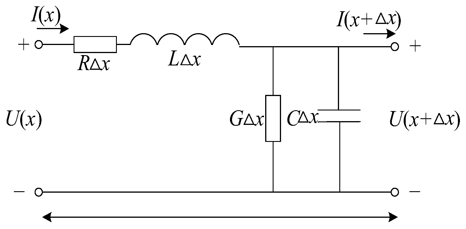
In the event of a fault in the photovoltaic system, the cable transmits high-frequency electromagnetic waves, so the lumped parameter cable model for low-frequency conditions is no longer applicable, and the busbar cable needs to be described by a distributed parameter model. A cable-equivalent circuit with distribution parameters is shown in Figure 3, where U means the voltage (V) signal. Hereby, it represents the voltage during an arc fault in a PV system. R indicates the cable resistance per unit length (Ω/m); L indicates the cable inductance per unit length (H/m); G indicates the cable conductance per unit length (S/m); C indicates the cable capacitance per unit length (F/m). The calculation formulas of the above parameters are shown in Equations (1)–(4) [18].

$$R\approx {\displaystyle \frac{1}{2\mathsf{\pi }}}\sqrt{{\displaystyle \frac{{\mu }_0\omega }{2}}}({\displaystyle \frac{1}{r_c}}\sqrt{{\rho }_{\mathrm{c}}}+{\displaystyle \frac{1}{r_s}}\sqrt{{\rho }_s})$$

(1)

$$L\approx {\displaystyle \frac{{\mu }_0}{2\mathsf{\pi }}}\mathit{ln}{\displaystyle \frac{r_{\mathrm{s}}}{r_{\mathrm{c}}}}+{\displaystyle \frac{1}{4\mathsf{\pi }}}\sqrt{{\displaystyle \frac{{\mu }_0\omega }{2}}}({\displaystyle \frac{1}{r_{\mathrm{c}}}}\sqrt{{\rho }_{\mathrm{c}}}+{\displaystyle \frac{1}{r_{\mathrm{s}}}}\sqrt{{\rho }_{\mathrm{s}}})$$

(2)

$$G={\displaystyle \frac{2\mathsf{\pi }\sigma }{\mathit{ln}(r_{\mathrm{s}}/r_{\mathrm{c}})}}$$

(3)

$$C={\displaystyle \frac{2\mathsf{\pi }\epsilon }{\mathit{ln}(r_{\mathrm{s}}/r_{\mathrm{c}})}}$$

(4)

where ω represents the angular frequency; μ₀ represents the magnetic permeability (under vacuum); r_c represents the radius of the conductor; ρ_c represents the resistivity of the conductor of the cable; r_s is the radius of the sheath of the cable; ρ_s is the resistivity of the cable shield; σ represents the conductivity of the insulation; ε is the dielectric constant of the insulation.

Based on the R, L, G and C parameters in Equations (1)–(4), the characteristic impedance Z₀ of the cable can be calculated as shown in Equation (5) [9].

$$Z_0=\sqrt{{\displaystyle \frac{R+j\omega L}{G+j\omega C}}}$$

(5)

4. Time Reversal of the Voltage Signal

As shown in Figure 1, voltage is used in this paper for arc fault location. When an arc fault occurs in a DC busbar cable of a PV system, the arc voltage signal travels along the cable. Sensors installed at the terminals receive voltage data containing arc information. The voltage data are reversed in time and resent back from the signal detection point to the cable line in the photovoltaic system. Various fault positions are assumed, which indicates different propagation distances of the reversed voltage. The location of the fault is then determined based on the waveform energy. The maximum energy where the fault is assumed indicates the position where the arc fault occurs. The principle of time reversal can be explained as below. Based on Figure 1,

$$u(x,t)-R\mathsf{\Delta }xi(x,t)-L\mathsf{\Delta }x{\displaystyle \frac{\partial i(x,t)}{\partial t}}-u(x+\mathsf{\Delta }x,t)=0$$

(6)

$$i\left(x,t\right)-G\mathsf{\Delta }xu\left(x+\mathsf{\Delta }x,t\right)-C\mathsf{\Delta }x{\displaystyle \frac{\partial u\left(x+\mathsf{\Delta }x,t\right)}{\partial t}}=i(x+\mathsf{\Delta }x,t)$$

(7)

where u(x,t) is the voltage at position x at moment t; i(x,t) is the current at position x at moment t.

By associating Equations (6) and (7) and assuming Δx→0, the following differential equation can be derived [19]:

$${\displaystyle \frac{\partial u(x,t)}{\partial x}}=-Ri(x,t)-L{\displaystyle \frac{\partial i(x,t)}{\partial t}}$$

(8)

$${\displaystyle \frac{\partial i(x,t)}{\partial x}}=-Gu(x,t)-C{\displaystyle \frac{\partial u(x,t)}{\partial t}}$$

(9)

From Equations (8) and (9), the voltage equation (ignoring cable losses) can be deduced as follows:

$${\displaystyle \frac{\partial u^2(x,t)}{\partial x^2}}-LC{\displaystyle \frac{\partial u^2(x,t)}{\partial t^2}}=0$$

(10)

Equation (11) is obtained by taking the opposite of t in Equation (10):

$${\displaystyle \frac{\partial u^2(x,-t)}{\partial x^2}}-LC{\displaystyle \frac{\partial u^2(x,-t)}{\partial t^2}}=0$$

(11)

Combining Equations (10) and (11) shows that if the solution of the voltage equation is u(x,t), then u(x, −t) is also a solution of this equation. In other words, without any losses, the voltage wave exhibits time-reversal symmetry during its propagation, which means that the voltage equation follows time-reversal symmetry.

In practice, the width of the time window is set to T, the corresponding voltage data collected by the sensor from the line terminals is u(x,t), and the time domain reversal operation for the voltage variable is shown in Equation (12):

$$u(x,t)\to u(x,T-t)$$

(12)

5. Arc Fault Location Using Time Reversal

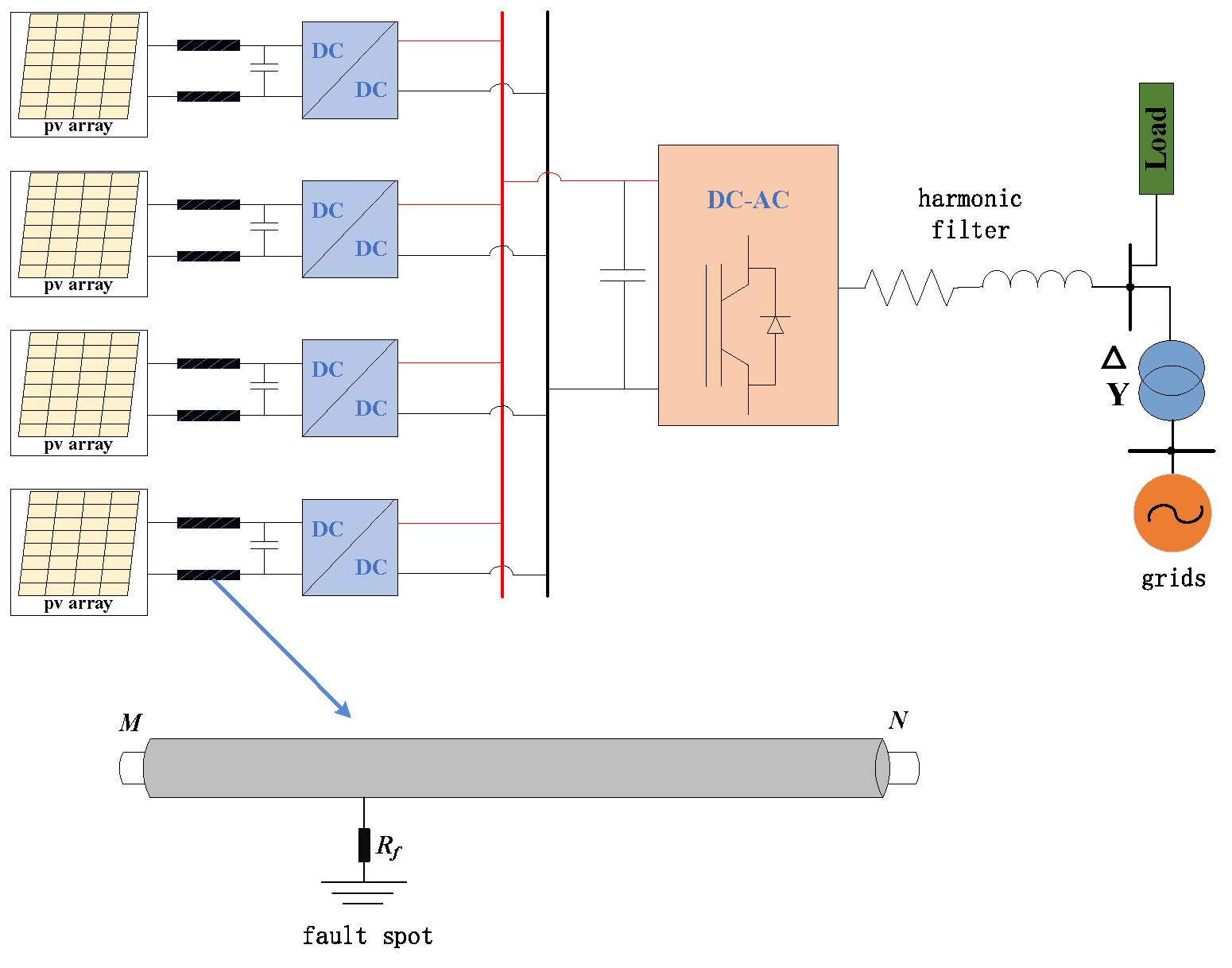
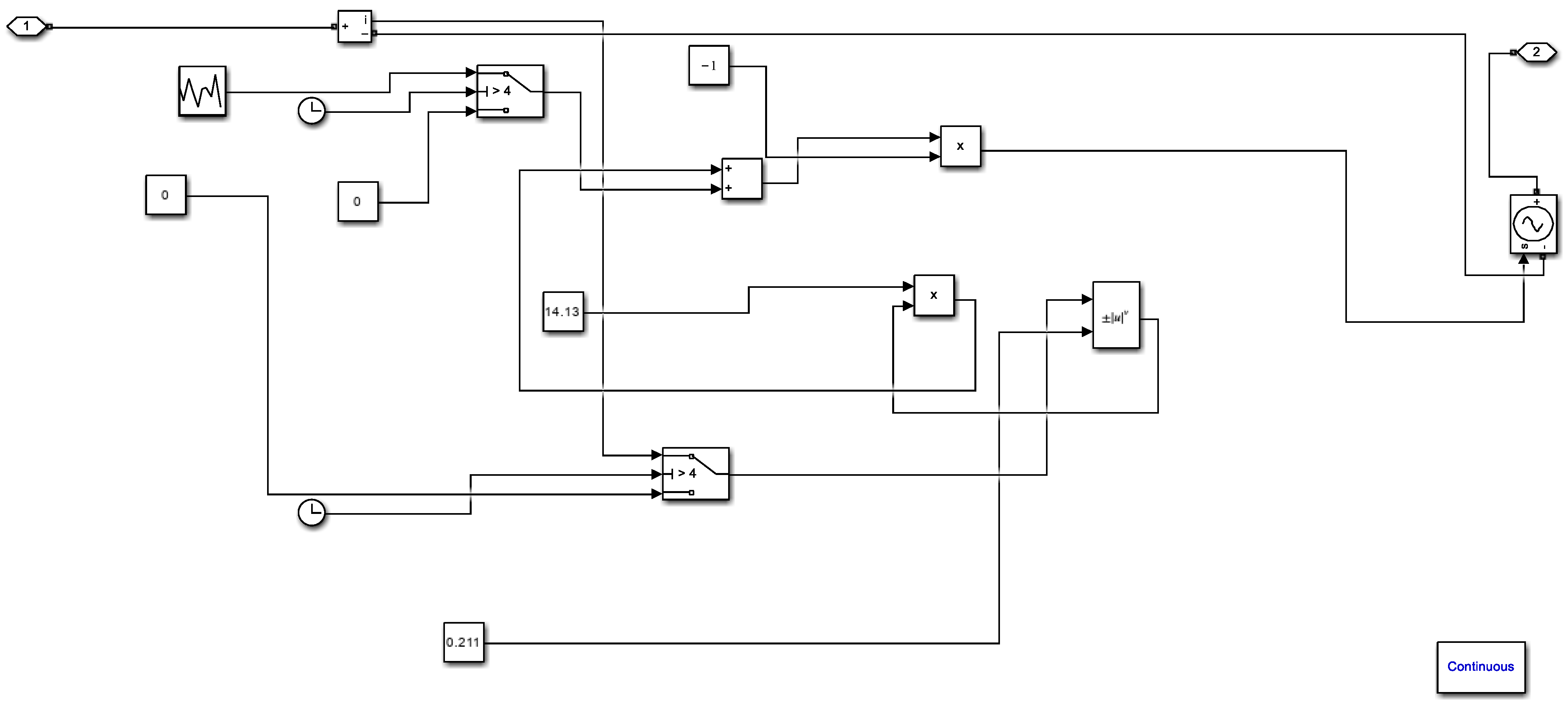
Figure 4 shows the PV system model, where the DC output of the PV module is 65 V, and it is converted up to 500 V DC via a DC/DC converter. Afterwards, the DC voltage of 500 V is converted by the DC/AC converter (inverter) to AC 35 kV through a transformer and connected to the grid. Assuming that the cable has an arc fault at position x at time t, the time domain voltage data with time during T are collected at the right end of the PV cable, labelled as N. In the figure, R_f is the grounded resistance at the fault point. The Paukert arc model is used here for arc generation, as shown in Figure 5. One hundred sets of simulations are performed, and the averaged result is used for evaluation. Each gap distance is used for 25 sets of data derivation.

A conjugation operation in the frequency domain enables the time reversal of time domain signals, which is a common method used in the time reversal process [20].

$$u(x,-t)\leftrightarrow U^{\mathrm{*}}(x,\omega )$$

(13)

The collected time domain voltage data at the right end of the PV cable carrying fault information for T time is transformed into frequency domain data analyzed with the following expression:

$$U_N(\omega )=H(x){·U}_f(\omega )$$

(14)

where H(x) denotes the transfer function from the arc fault voltage U_f to the N-terminal detection.

The time domain data collected by the sensor at the N-terminal is reversed to obtain its frequency expression as $U_N^{\mathrm{*}}(\omega )$. According to the principle of the Norton equivalent circuit, the corresponding current value can be obtained as $I_N^{\mathrm{*}}(\omega )$.

$$I_N^{\mathrm{*}}(\omega )={\displaystyle \frac{U_N^{\mathrm{*}}(\omega )}{Z_M}}$$

(15)

where Z_M is the equivalent impedance at the N-terminal. The data processed by time reversion at the N-terminal are transmitted back to the cable line, assuming a current signal at the fault point x_f′:

$$I_f\left(x_f^{\prime },\omega \right)=H(x_f^{\prime })·I_N^{\mathrm{*}}(\omega )$$

(16)

The current normalized energy values for the hypothetical fault points are calculated sequentially as shown in Equation (17):

$$P\left(x_f^{\prime }\right)=\sum _{j=1}^N{i}_{x_f^{\prime }}^2(j)$$

(17)

Equation (17) gives the maximum value of current energy at $x_f^{\prime }$; i.e., $x_f=x_f^{\prime }$.

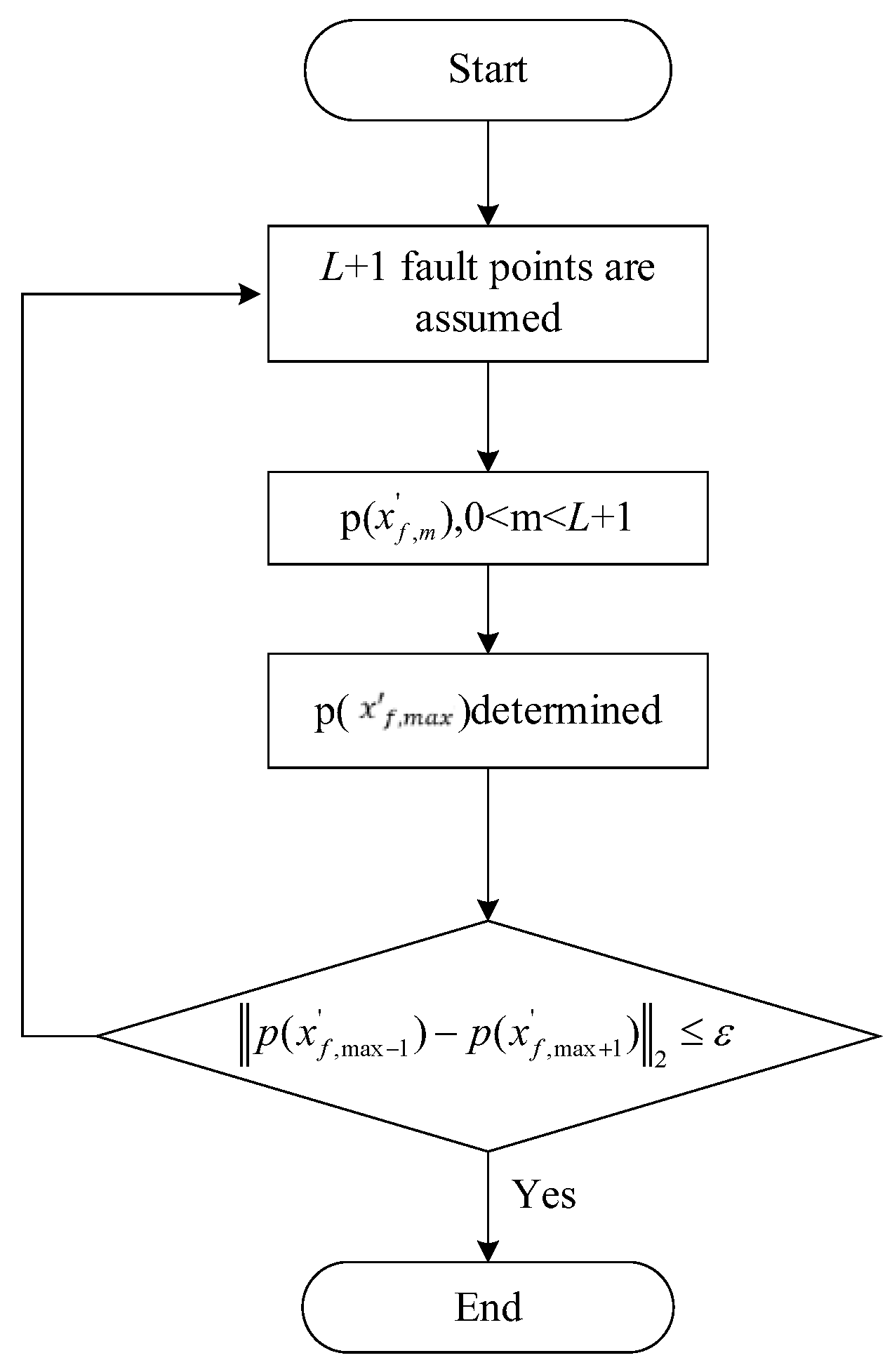
In order to find the fault with the largest energy value, the specific location process is shown in Figure 6. Firstly, L + 1 fault points are assumed along the cable line. The current energy value is calculated based on the time reversal of each hypothetical fault point in turn. The fault point $x_{f,max}^{\prime }$ with the largest energy value indicates the fault location. The error is calculated by ${‖p(x_{f,\mathit{max}-1}^{\prime })-p(x_{f,\mathit{max}+1}^{\prime })‖}_2$ to determine whether it is smaller than $\epsilon$, which is the positioning accuracy. More fault points are tested with the above operation until the positioning accuracy is satisfied. In the end, the point with the largest energy value corresponds to the real fault point.

6. Simulation Results and Analysis

The simulation model takes the cable between the PV array and the booster module as an example. The cable parameters between the PV array and the booster module are set as below. The total cable length is 1 km. The value of the cable’s unit-distributed inductance L is 0.56 mH/km. The value of the unit-distributed capacitance C is 0.09 μF/km. The value of the transmission line’s unit-distributed resistance R is 0.112 Ω/km, and the conductance is negligible.

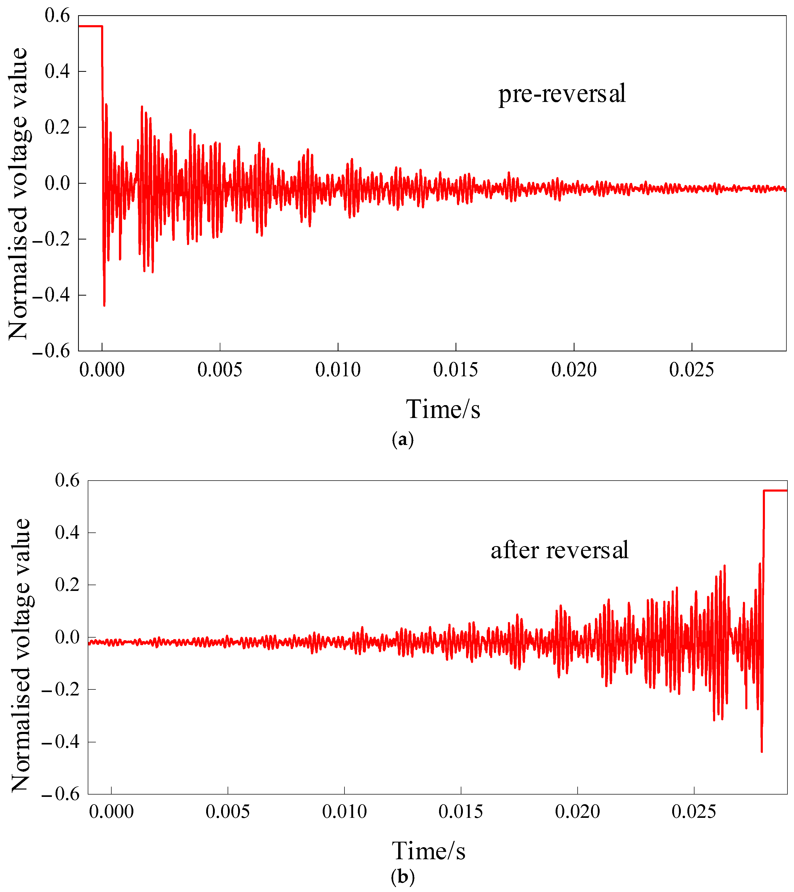
It is assumed that a grounded arc fault occurs at a distance of 0.7 km from the N-terminal. The voltage signal from the arc fault will propagate along the cable, and the sensor set up at the N-terminal will receive the voltage data with the defect location information. Therefore, the collected voltage data will be processed into current data according to the time reversal and returned in the original path. By normalizing the value at the preset fault points, the point with the largest value of normalized current energy is the original fault location. The normalized voltage data waveform before and after time reversal is shown in Figure 7, with a sampling frequency of 20 kHz. It is obvious that the reversed signal is symmetric to the original one.

In order to investigate whether the transition resistance has any effect on the localization method, the grounded resistance R_f of 1 Ω, 5 Ω, and 10 Ω, respectively, is set for this study. Figure 8 shows the calculated current energy values at the fault point with different grounded resistances.

It can be seen that the fault point with the largest energy value is 0.7 km, which refers to the set value. It can be seen that the size of the grounded resistance has an effect on the localization results. With the increase in the impedance value, the significance of the fault location decreases. This is because when the grounded resistance reaches a higher value, it approaches the characteristic impedance of the cable, while, in general, a fault with high grounded impedance is more difficult to locate. This also matches the observed result in the paper.

In order to study this further, two more fault points of 0.3 km and 0.5 km are set up, respectively. Furthermore, the cable length is varied to check the performance of the location method. The location method is used to find out the specific fault point with the calculated maximum energy value, as shown in

Table 2. Location results for different failures.

Fault Location	Calculated Result	Error
0.3 km@1 km	0.298 km	0.67%
0.3 km@2 km	0.290 km	0.50%
0.3 km@3 km	0.282 km	0.60%
0.5 km@1 km	0.5 km	0%
0.5 km@2 km	0.491 km	0.45%
0.5 km@3 km	0.485 km	0.50%
0.7 km@1 km	0.699 km	0.10%
0.7 km@2 km	0.686 km	0.70%
0.7 km@3 km	0.681 km	0.63%

. The error of the three cases is 0.7% at most, which shows that the use of the cable fault location method based on time reversal is capable of identifying the fault in the whole range of the cable section, which verifies the correctness of the proposed method in this paper.

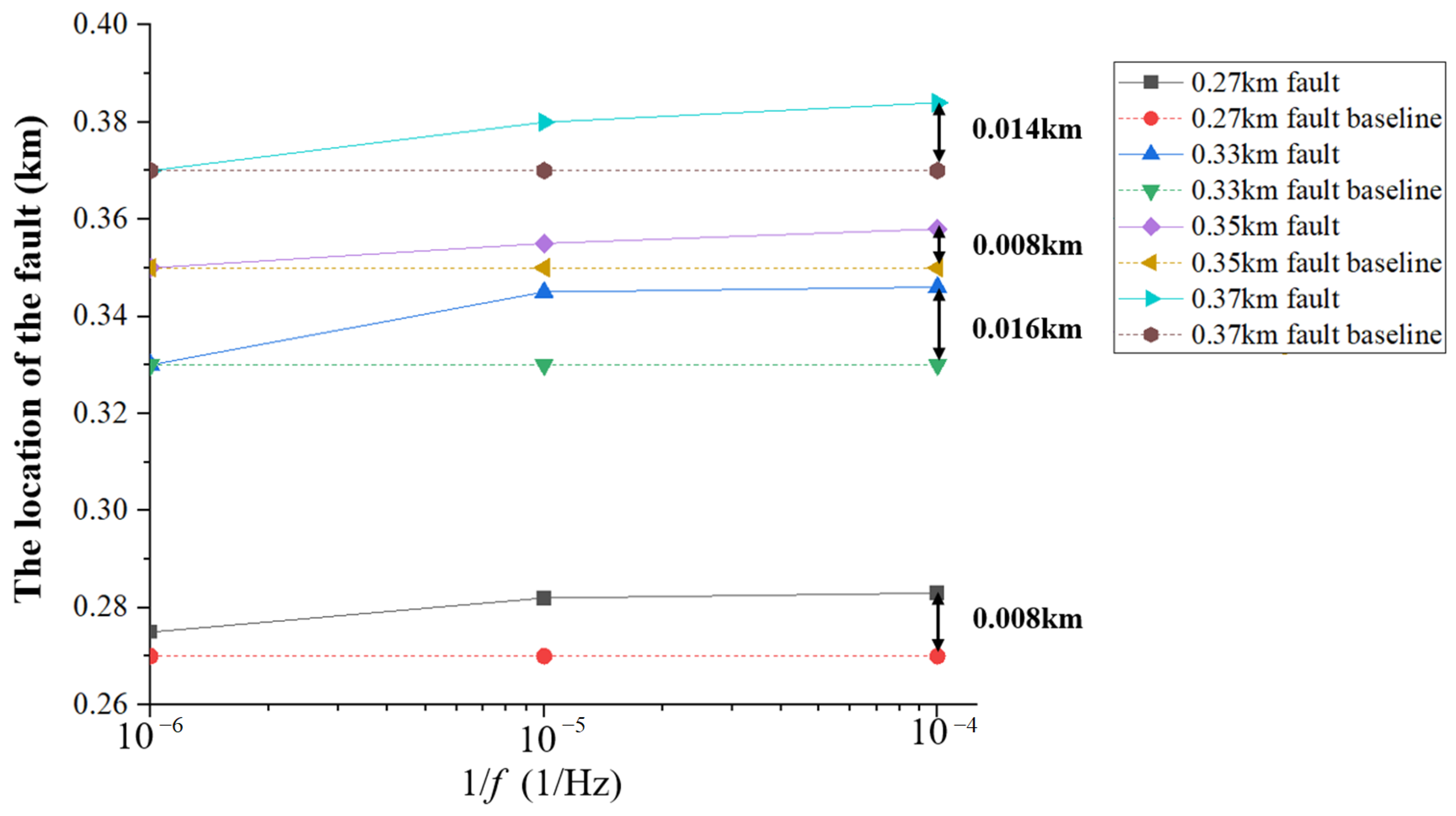
Another affecting factor, the sampling frequency, is varied to observe its influence on the location accuracy. The result is shown in Figure 9. Again, three scenarios are tested, and it is observed that with the decrease in the sampling frequency, the location accuracy also degrades. This analysis can help to determine the suitable sampling frequency based on performance demand and cost limitation. It should be noted that compared with previous studies, e.g., up to 20 MHz in [21] and 100 kHz in [11], setting the sampling frequency down to 10 kHz still yields a location error of less than 5%. This has significant engineering meaning, since the recorder’s cost can be reduced greatly.

To sum up, the time reversal method is suitalbe for DC arc fault location in PV cables. To implement this method in practice, a transistent voltage sensor needs to be installed at the end of the cable. The sampling frequency can be chosen based on the result in Figure 9 based on the demanded location accuracy and cost. The time reversal method can be implemented in an embeded system, e.g., FPGA, for real-time operation.

7. Conclusions

In this paper, a cable arc fault location method for photovoltaic systems is proposed based on the principle of time reversal. The arc fault waveform is collected via a DC arc test platform. The Paukert arc model is utilized to simulate the arc phenomenon. A PV system with a cable arc fault is established. When an arc fault occurs in a PV system, the sensor will collect the voltage signal of the fault at one of the line terminals. The acquired voltage wave is equivalently converted into a current wave, which is transmitted from the line terminal back to the cable line in the original way, forming a symmetrical propagation path as the original arc fault travels along the cable. For each hypothetical fault location, the normalized energy value of the current from the observation point is calculated. The maximum current energy value with the pre-assumed location refers to the real fault location. The grounded resistance, fault location and sampling frequency are analyzed as the affecting factors. All studies verify the effectiveness and accuracy of the method to locate arc faults in PV system cables. In the future, field verification is planned with the proposed method.