Option Pricing Formulas of Uncertain Mean-Reverting Stock Model with Symmetry Analysis

Abstract

With the development of uncertain finance, uncertain stock models have become increasingly popular for modeling stock prices. This paper explores the symmetric properties inherent in the uncertain mean-reverting stock model, particularly in the structure of its differential equations and the resulting pricing formulas. The primary findings comprise the derivation of explicit pricing formulas, via uncertain differential equations, for European, American, Asian, and geometric average Asian options under the uncertain mean-reverting stock model. The symmetry in the inverse uncertainty distributions and the duality between call and put options are highlighted, demonstrating the model’s alignment with symmetric financial principles. Furthermore, several numerical examples are provided to illustrate the applicability and the symmetry-related characteristics of the derived formulas.

1. Introduction

Uncertain finance theory is an alternative to stochastic finance theory on the basis of the uncertainty theory proposed by Liu [1] in 2007. Stochastic finance theory assumes that stock prices follow stochastic differential equations, but Liu [2] pointed out that using stochastic differential equations to model stock prices would derive a paradox. Up to now, numerous empirical examples have been shown to verify this viewpoint, such as stock prices (Liu and Liu [3], Liu and Liu [4]), the Shanghai interbank offered rate (Yang and Ke [5]), US the Dollar to Chinese Yuan exchange rate (Ye and Liu [6]), etc. Therefore, instead of using stochastic differential equations to model stock prices, uncertain differential equations are being used by more and more scholars.

The landscape of uncertain finance has been recently mapped by a systematic review (Yang and Li [7]), which synthesizes the field’s theoretical advances and empirical applications. In light of this overview, our work seeks to advance the discourse by establishing a unified framework for pricing a suite of options under the mean-reverting stock model. A key distinctive feature of our approach is its emphasis on symmetry analysis, a perspective that remains underexplored in the existing literature. This methodological focus provides a novel lens to unify and simplify derivative pricing, addressing a recognized need for greater model generalization and theoretical elegance.

Moreover, the concept of symmetry plays a significant role in financial modeling, particularly in the formulation and solution of differential equations governing asset prices. In this paper, we emphasize the symmetric structure of the uncertain mean-reverting model, which exhibits time-reversal symmetry in its mean-reverting property and payoff symmetries between call and put options. Such symmetries not only simplify the derivation of pricing formulas but also enhance the model’s theoretical consistency and practical applicability. By integrating symmetry principles into uncertain finance, this study contributes to a deeper understanding of the structural beauty and balance in financial derivative pricing.

Although Peng and Yao [8] presented the uncertain mean-reverting stock model in 2011, the derivation procedure in that paper was based on another stock model. Moreover, Tian et al. [9] and Tian et al. [10] made some mistakes in obtaining the inverse uncertainty distribution of stock prices. The purpose of this study is to establish a unified analytical framework for option pricing under the uncertain mean-reverting model. Our contribution to the literature is threefold: first, we provide a rigorous derivation of the pricing formulas; second, we introduce a novel symmetry analysis that simplifies and unifies the understanding of these formulas; and third, we demonstrate the model’s versatility by applying it to four fundamental option types—European (path-independent), American (early-exercise), and both arithmetic and geometric Asian options (path-dependent)—thereby offering a comprehensive toolkit for both theorists and practitioners. This is a theoretical study, and as such, the analysis relies on numerical experiments to illustrate the properties of the derived formulas.

The organization of the rest of this paper is as follows: Section 2 reviews the relevant literature and some aspects of uncertain differential equations that will be used in this paper. Section 3 details the methodology and derives the pricing formulas for various options, including a dedicated symmetry analysis. Section 4 presents a numerical analysis and discussion of the results. At last, Section 5 draws the conclusion and suggests directions for future research.

2. Literature Review and Theoretical Preliminaries

As an aspect of financial products, a large variety of stock options have been successfully applied using uncertain finance theory. In 2009, an uncertain exponential stock model was first proposed by Liu [11] based on uncertain differential equations, and they derived the prices of European options. Following that, the prices of American options were obtained by Chen [12] in 2011, and the prices of Asian options were given by Sun and Chen [13] in 2015. Meanwhile, the prices of geometric average Asian options were studied by Zhang and Liu [14] in 2014, and the prices of European vulnerable options were investigated by Cao [15] in 2013. Furthermore, numerous other option pricing problems of the uncertain exponential stock model were investigated based on uncertain finance theory, including barrier options (Yao and Qin [16]), power options (Zhang et al. [17]), lookback options (Zhang et al. [18]), Asian barrier options (Yang et al. [19]), American barrier options (Gao et al. [20]), geometric Asian barrier options (Gao et al. [21]), barrier-lookback options (Gao and Jia [22]), Bermudan options (Pan et al. [23]), binary options (Yang and Gao [24]), and so on.

In addition to the uncertain exponential stock model proposed by Liu [11], many uncertain stock models have been successfully adopted for stock options. For instance, Peng and Yao [8] presented an uncertain mean-reverting stock model and priced European and American options based on it in 2011. Under this model, Tian et al. [9] provided the prices of barrier options, and Tian et al. [10] gave the prices of lookback options. Simultaneously, Zhang et al. [18] researched the prices of lookback options, and Pan et al. [23] studied the prices of Bermudan options based on another type of uncertain mean-reverting stock model. Sun and Su [25] proposed a new model with a floating interest rate and priced European and American options based on it in 2017. Under this model, Sun et al. [26] obtained the prices of Asian options, and Pan et al. [23] studied the prices of Bermudan options. In addition, Ji and Zhou [27] proposed an uncertain stock model with jumps and priced European options based on it in 2015. Moreover, Dai et al. [28] presented an uncertain exponential Ornstein–Uhlenbeck stock model and priced European and American options based on it in 2017. After that, Gao et al. [29] studied the prices of lookback options determined by the model in 2018. Recently, Liu and Lio [30] investigated the prices of power options determined by the model in 2024. Furthermore, an uncertain volatility model was proposed by Hassanzadeh and Mehrdoust [31], and the prices of European options were obtained based on it.

Assume $X_t$ is the bond price, $Y_t$ is the stock price, r is the riskless interest rate, and $C_t$ is a Liu process. In 2009, Liu [11] first proposed an uncertain exponential stock model as follows:

$$\left\{\begin{array}{c}\mathrm{d}{X}_t=r{X}_t\mathrm{d}t\hfill \\ \mathrm{d}{Y}_t=e{Y}_t\mathrm{d}t+\sigma Y_t\mathrm{d}{C}_t\hfill \end{array}\right.$$

where e and $\sigma$ are given constants with $\sigma >0$. After that, in 2011, Peng and Yao [8] proposed an uncertain mean-reverting stock model as follows:

$$\left\{\begin{array}{c}\mathrm{d}{X}_t=r{X}_t\mathrm{d}t\hfill \\ \mathrm{d}{Y}_t=(m-a{Y}_t)\mathrm{d}t+\sigma Y_t\mathrm{d}{C}_t\hfill \end{array}\right.$$

(1)

where $m,a$ and $\sigma$ are given constants with $m>0$ and $\sigma >0$. In this section, we will show some useful conclusions for obtaining some option pricing formulas of the stock model (1).

Theorem 1

(Yao and Chen [32]). An α-path $X_t^{\alpha }$ for the uncertain differential equation

$$\mathrm{d}{X}_t=f(t,X_t)\mathrm{d}t+g(t,X_t)\mathrm{d}{C}_t$$

(2)

is the solution of

$$\mathrm{d}{X}_t^{\alpha }=f(t,X_t^{\alpha })\mathrm{d}t+\left|g(t,X_t^{\alpha })\right|{\Phi }^{-1}\left(\alpha \right)\mathrm{d}t$$

where

$${\Phi }^{-1}\left(\alpha \right)={\displaystyle \frac{\sqrt{3}}{\pi }}ln{\displaystyle \frac{\alpha }{1-\alpha }}.$$

Theorem 2

(Yao and Chen [32]). The solution of the uncertain differential Equation (2) has an inverse uncertainty distribution

$${\Psi }_t^{-1}\left(\alpha \right)=X_t^{\alpha }$$

where $X_t^{\alpha }$ is the α-path.

Lemma 1

(Peng and Yao [8]). The solution of a linear uncertain differential equation

$$\mathrm{d}{X}_t=\left(m-a{X}_t\right)\mathrm{d}t+\sigma X_t\mathrm{d}{C}_t$$

is

$$X_t=\exp \left(-at+\sigma C_t\right)\left(X_0+m{\int }_0^t\exp \left(as-\sigma C_s\right)\mathrm{d}s\right).$$

3. Methodology and Option Pricing Formulas

3.1. European Option Pricing

The pricing formulas for European call and put options exhibit a natural symmetry through the put–call parity relation, which is preserved even under the uncertain mean-reverting framework. This symmetry reflects the balanced risk structure between buying and selling rights under uncertainty. This section aims to obtain the pricing formulas of European options in an uncertain environment. A European call option is a type of option contract that enables the investor to buy stock at an expiration time s with a strike price K. In 2009, Liu [11] found that the price of a European call option is

$$f_{ec}=\exp (-rs)E\left[{\left(Y_s-K\right)}^{+}\right]$$

(3)

based on the fair price principle.

Theorem 3.

Assume that a European call option for the uncertain mean-reverting stock model (1), where $m,a,\sigma$ and r are parameters with $m>0$ and $\sigma >0$, has a strike price K and an expiration time s. Then, the European call option price is

$$f_{ec}=\exp (-rs){\int }_0^1{\left(\exp \left(\nu \left(\alpha \right)s\right)Y_0+{\displaystyle \frac{\left(\exp \right(\nu \left(\alpha \right)s)-1)m}{\nu \left(\alpha \right)}}-K\right)}^{+}\mathrm{d}\alpha$$

(4)

where $\nu \left(\alpha \right)$ is the inverse uncertainty distribution of $\mathcal{N}(-a,\sigma )$, i.e.,

$$\nu \left(\alpha \right)={\displaystyle \frac{\sqrt{3}\sigma }{\pi }}ln{\displaystyle \frac{\alpha }{1-\alpha }}-a.$$

Proof. 

It follows from Theorem 1 that the $\alpha$-path $Y_s^{\alpha }$ of the stock price $Y_s$ is the solution of

$$\mathrm{d}{Y}_s^{\alpha }=(m-a{Y}_s^{\alpha })\mathrm{d}t+\left|\sigma Y_s^{\alpha }\right|{\displaystyle \frac{\sqrt{3}}{\pi }}ln{\displaystyle \frac{\alpha }{1-\alpha }}\mathrm{d}t.$$

(5)

Moreover, it follows from Lemma 1 that

$$Y_s=\exp \left(-as+\sigma C_s\right)\left(Y_0+m{\int }_0^s\exp \left(at-\sigma C_t\right)\mathrm{d}t\right).$$

Since $Y_0$ and m are positive numbers, we find that $Y_s$ is a positive uncertain variable. Furthermore, it follows from Theorem 2 that

$$Y_s^{\alpha }={\Psi }_s^{-1}\left(\alpha \right)$$

where ${\Psi }_s^{-1}$ is the inverse uncertainty distribution of $Y_s$. Thus $Y_s^{\alpha }$ is also a positive number. Since $\sigma$ is also a positive number, (5) can be rewritten as

$$\mathrm{d}{Y}_s^{\alpha }=(m-a{Y}_s^{\alpha })\mathrm{d}t+\sigma Y_s^{\alpha }{\displaystyle \frac{\sqrt{3}}{\pi }}ln{\displaystyle \frac{\alpha }{1-\alpha }}\mathrm{d}t.$$

(6)

That is,

$${\displaystyle \frac{\mathrm{d}{Y}_s^{\alpha }}{\mathrm{d}t}}=\nu \left(\alpha \right)Y_s^{\alpha }+m$$

(7)

where

$$\nu \left(\alpha \right)={\displaystyle \frac{\sqrt{3}\sigma }{\pi }}ln{\displaystyle \frac{\alpha }{1-\alpha }}-a.$$

Since (7) is a first-order nonhomogeneous ordinary differential equation, we obtain

$$\begin{array}{cc}\hfill Y_s^{\alpha }& =\exp \left({\int }_0^s\nu \left(\alpha \right)\mathrm{d}t\right)Y_0^{\alpha }+{\int }_0^{s}m\exp \left({\int }_t^s\nu \left(\alpha \right)\mathrm{d}r\right)\mathrm{d}t\hfill \\ & =\exp \left(\nu \left(\alpha \right)s\right)Y_0+m{\int }_0^s\exp \left((s-t)\nu \left(\alpha \right)\right)\mathrm{d}t.\hfill \end{array}$$

We write

$${\alpha }^{*}={\displaystyle \frac{1}{1+\exp \left(-{\displaystyle \frac{a\pi }{\sqrt{3}\sigma }}\right)}}.$$

Then

$$\nu \left({\alpha }^{*}\right)=0.$$

Thus

$$\begin{array}{c}\hfill Y_s^{{\alpha }^{*}}=Y_0+m{\int }_0^{s}1\mathrm{d}t=Y_0+ms\end{array}$$

and

$$\begin{array}{cc}\hfill Y_s^{\alpha }& =\exp \left(\nu \left(\alpha \right)s\right)Y_0+m{\int }_0^s\exp \left((s-t)\nu \left(\alpha \right)\right)\mathrm{d}t\hfill \\ & =\exp \left(\nu \left(\alpha \right)s\right)Y_0+{\displaystyle \frac{\left(\exp \right(\nu \left(\alpha \right)s)-1)m}{\nu \left(\alpha \right)}}\hfill \end{array}$$

for any $\alpha \ne {\alpha }^{*}$. According to the inverse uncertainty distribution formula, the inverse uncertainty distribution of ${\left(Y_s-K\right)}^{+}$ is

$${{\rm Y}}_s^{-1}\left({\alpha }^{*}\right)={\left(Y_0+ms-K\right)}^{+}$$

and

$${{\rm Y}}_s^{-1}\left(\alpha \right)={\left(\exp \left(\nu \left(\alpha \right)s\right)Y_0+{\displaystyle \frac{\left(\exp \right(\nu \left(\alpha \right)s)-1)m}{\nu \left(\alpha \right)}}-K\right)}^{+}$$

for any $\alpha \ne {\alpha }^{*}$. Furthermore,

$$\underset{\alpha \to {\alpha }^{*}}{lim}{\left(\exp \left(\nu \left(\alpha \right)s\right)Y_0+{\displaystyle \frac{\left(\exp \right(\nu \left(\alpha \right)s)-1)m}{\nu \left(\alpha \right)}}-K\right)}^{+}={\left(Y_0+ms-K\right)}^{+}.$$

By using (3) and the expected value formula, we obtain

$$f_{ec}=\exp (-rs){\int }_0^1{\left(\exp \left(\nu \left(\alpha \right)s\right)Y_0+{\displaystyle \frac{\left(\exp \right(\nu \left(\alpha \right)s)-1)m}{\nu \left(\alpha \right)}}-K\right)}^{+}\mathrm{d}\alpha .$$

A European put option is a type of option contract that enables the investor to sell stock at an expiration time s with a strike price K. In 2009, Liu [11] found that the price of a European put option is

$$f_{ep}=\exp (-rs)E\left[{\left(K-Y_s\right)}^{+}\right]$$

(8)

based on the fair price principle. □

Theorem 4.

Assume that a European put option for the uncertain mean-reverting stock model (1), where $m,a,\sigma$ and r are parameters with $m>0$ and $\sigma >0$, has a strike price K and an expiration time s. Then the European put option price is

$$f_{ep}=\exp (-rs){\int }_0^1{\left(K-\exp \left(\nu \left(\alpha \right)s\right)Y_0-{\displaystyle \frac{\left(\exp \right(\nu \left(\alpha \right)s)-1)m}{\nu \left(\alpha \right)}}\right)}^{+}\mathrm{d}\alpha$$

(9)

where $\nu \left(\alpha \right)$ is the inverse uncertainty distribution of $\mathcal{N}(-a,\sigma )$, i.e.,

$$\nu \left(\alpha \right)={\displaystyle \frac{\sqrt{3}\sigma }{\pi }}ln{\displaystyle \frac{\alpha }{1-\alpha }}-a.$$

Proof. 

It follows from Theorem 3 that the inverse uncertainty distribution of stock price $Y_s$ is

$${\Psi }_s^{-1}\left({\alpha }^{*}\right)=Y_0+ms$$

and

$${\Psi }_s^{-1}\left(\alpha \right)=\exp \left(\nu \left(\alpha \right)s\right)Y_0+{\displaystyle \frac{\left(\exp \right(\nu \left(\alpha \right)s)-1)m}{\nu \left(\alpha \right)}}$$

for any $\alpha \ne {\alpha }^{*}$, where

$${\alpha }^{*}={\displaystyle \frac{1}{1+\exp \left(-{\displaystyle \frac{a\pi }{\sqrt{3}\sigma }}\right)}}$$

and

$$\nu \left(\alpha \right)={\displaystyle \frac{\sqrt{3}\sigma }{\pi }}ln{\displaystyle \frac{\alpha }{1-\alpha }}-a.$$

Thus the inverse uncertainty distribution of ${\left(K-Y_s\right)}^{+}$ is

$${{\rm Y}}_s^{-1}(1-{\alpha }^{*})={\left(K-Y_0-ms\right)}^{+}$$

and

$${{\rm Y}}_s^{-1}\left(\alpha \right)={\left(K-\exp \left(\nu (1-\alpha )s\right)Y_0-{\displaystyle \frac{\left(\exp \right(\nu (1-\alpha )s)-1)m}{\nu (1-\alpha )}}\right)}^{+}$$

for any $\alpha \ne 1-{\alpha }^{*}$. Furthermore,

$$\underset{\alpha \to 1-{\alpha }^{*}}{lim}{\left(K-\exp \left(\nu (1-\alpha )s\right)Y_0-{\displaystyle \frac{\left(\exp \right(\nu (1-\alpha )s)-1)m}{\nu (1-\alpha )}}\right)}^{+}={\left(K-Y_0-ms\right)}^{+}.$$

By using (8), we obtain

$$\begin{array}{cc}\hfill f_{ep}& =\exp (-rs)E\left[{\left(K-Y_s\right)}^{+}\right]\hfill \\ & =\exp (-rs){\int }_0^1{\left(K-\exp \left(\nu (1-\alpha )s\right)Y_0-{\displaystyle \frac{\left(\exp \right(\nu (1-\alpha )s)-1)m}{\nu (1-\alpha )}}\right)}^{+}\mathrm{d}\alpha \hfill \\ & =\exp (-rs){\int }_0^1{\left(K-\exp \left(\nu \left(\alpha \right)s\right)Y_0-{\displaystyle \frac{\left(\exp \right(\nu \left(\alpha \right)s)-1)m}{\nu \left(\alpha \right)}}\right)}^{+}\mathrm{d}\alpha .\hfill \end{array}$$

□

3.2. Symmetry Analysis

The uncertain mean-reverting model exhibits profound symmetric properties that provide crucial insights into the structural relationships between different financial derivatives. Our symmetry analysis reveals how these inherent balances simplify the derivation of pricing formulas and enhance the model’s theoretical consistency.

The most prominent symmetry in our framework is the put–call duality, which establishes a fundamental relationship between call and put options under uncertainty. For European options, this duality manifests through complementary inverse uncertainty distributions:

$$\begin{array}{c}{f}_{ec}=\exp (-rs){\int }_0^1{\left({\Psi }_s^{-1}\left(\alpha \right)-K\right)}^{+}d\alpha ,\\ f_{ep}=\exp (-rs){\int }_0^1{\left(K-{\Psi }_s^{-1}(1-\alpha )\right)}^{+}d\alpha ,\end{array}$$

where ${\Psi }_s^{-1}$ is the inverse uncertainty distribution of stock price $Y_s$. This elegant mathematical structure demonstrates that the pricing of call and put options are intrinsically linked through a simple transformation of $\alpha$ to $1-\alpha$. The same inverse uncertainty distribution ${\Psi }_s^{-1}$ serves both option types, highlighting the balanced risk structure between buying and selling rights in uncertain markets.

In the following subsections, we will see that similar put–call symmetries also exist for American options, Asian options, and geometric average Asian options.

3.3. American Option Pricing

American options introduce an early exercise feature, which breaks the time-homogeneity symmetry characteristic of European options. However, the inverse uncertainty distributions used in our pricing method maintain a symmetric form in the spatial domain, allowing for efficient evaluation of the optimal stopping problem. This section aims to obtain the pricing formulas of American options in an uncertain environment. An American call option is a type of option contract that enables the investor to buy stock at any time ahead of an expiration time s with a strike price K. In 2011, Chen [12] found that the price of an American call option is

$$f_{amc}=E\left[\underset{0\le t\le s}{sup}\exp (-rt){\left(Y_t-K\right)}^{+}\right]$$

(10)

based on the fair price principle.

Theorem 5.

Assume that an American call option for the uncertain stock model (1), where $m,a,\sigma$ and r are parameters with $m>0$ and $\sigma >0$, has a strike price K and an expiration time s. Then the American call option price is

$$f_{amc}={\int }_0^{1}G\left(\alpha \right)\mathrm{d}\alpha$$

(11)

where

$$G\left(\alpha \right)=\left\{\begin{array}{cc}{\displaystyle g(0,\alpha )\vee g\left(\tau \right(\alpha ),\alpha )\vee g(s,\alpha ),}& if 0<\tau \left(\alpha \right)<s\hfill \\ {\displaystyle g(0,\alpha )\vee g(s,\alpha ),}& otherwise,\hfill \end{array}\right.$$

$$g(t,\alpha )=\exp (-rt){\left(\exp \left(\nu \left(\alpha \right)t\right)Y_0+{\displaystyle \frac{\left(\exp \right(\nu \left(\alpha \right)t)-1)m}{\nu \left(\alpha \right)}}-K\right)}^{+},$$

$$\tau \left(\alpha \right)={\displaystyle \frac{1}{\nu \left(\alpha \right)}}ln{\displaystyle \frac{r\left(m+\nu \left(\alpha \right)K\right)}{(r-\nu \left(\alpha \right))\left(m+\nu \left(\alpha \right)Y_0\right)}},$$

$$\nu \left(\alpha \right)={\displaystyle \frac{\sqrt{3}\sigma }{\pi }}ln{\displaystyle \frac{\alpha }{1-\alpha }}-a.$$

Proof. 

It follows from Theorem 3 that the inverse uncertainty distribution of stock price $Y_s$ is

$${\Psi }_s^{-1}\left({\alpha }^{*}\right)=Y_0+ms$$

and

$${\Psi }_s^{-1}\left(\alpha \right)=\exp \left(\nu \left(\alpha \right)s\right)Y_0+{\displaystyle \frac{\left(\exp \right(\nu \left(\alpha \right)s)-1)m}{\nu \left(\alpha \right)}}$$

for any $\alpha \ne {\alpha }^{*}$, where

$${\alpha }^{*}={\displaystyle \frac{1}{1+\exp \left(-{\displaystyle \frac{a\pi }{\sqrt{3}\sigma }}\right)}}$$

and

$$\nu \left(\alpha \right)={\displaystyle \frac{\sqrt{3}\sigma }{\pi }}ln{\displaystyle \frac{\alpha }{1-\alpha }}-a.$$

Since $\exp (-rt){(Y_t-K)}^{+}$ is an increasing function of $Y_t$, the inverse uncertainty distribution of

$$\underset{0\le t\le s}{sup}\exp (-rt){\left(Y_t-K\right)}^{+}$$

is

$${{\rm Y}}_s^{-1}\left({\alpha }^{*}\right)=\underset{0\le t\le s}{sup}\exp (-rt){\left(Y_0+mt-K\right)}^{+}$$

and

$${{\rm Y}}_s^{-1}\left(\alpha \right)=\underset{0\le t\le s}{sup}\exp (-rt){\left(\exp \left(\nu \left(\alpha \right)t\right)Y_0+{\displaystyle \frac{\left(\exp \right(\nu \left(\alpha \right)t)-1)m}{\nu \left(\alpha \right)}}-K\right)}^{+}$$

for any $\alpha \ne {\alpha }^{*}$. Furthermore,

$$\begin{array}{cc}& \underset{\alpha \to {\alpha }^{*}}{lim}\underset{0\le t\le s}{sup}\exp (-rt){\left(\exp \left(\nu \left(\alpha \right)t\right)Y_0+{\displaystyle \frac{\left(\exp \right(\nu \left(\alpha \right)t)-1)m}{\nu \left(\alpha \right)}}-K\right)}^{+}\hfill \\ \hfill =& \underset{0\le t\le s}{sup}\exp (-rt){\left(Y_0+mt-K\right)}^{+}.\hfill \end{array}$$

By using (10), we obtain

$$\begin{array}{c}\hfill f_{amc}={\int }_0^1\underset{0\le t\le s}{sup}\exp (-rt){\left(\exp \left(\nu \left(\alpha \right)t\right)Y_0+{\displaystyle \frac{\left(\exp \right(\nu \left(\alpha \right)t)-1)m}{\nu \left(\alpha \right)}}-K\right)}^{+}\mathrm{d}\alpha .\end{array}$$

For further simplification, we take

$$h(t,\alpha )=\exp (-rt)\left(\exp \left(\nu \left(\alpha \right)t\right)Y_0+{\displaystyle \frac{\left(\exp \right(\nu \left(\alpha \right)t)-1)m}{\nu \left(\alpha \right)}}-K\right)$$

where $0\le t\le s$ and $0<\alpha <1$. Then

$${\displaystyle \frac{\partial h(t,\alpha )}{\partial t}}=\exp (-rt)\left(\left({\displaystyle \frac{m}{\nu \left(\alpha \right)}}+Y_0\right)(\nu \left(\alpha \right)-r)\exp \left(\nu \left(\alpha \right)t\right)+r\left({\displaystyle \frac{m}{\nu \left(\alpha \right)}}+K\right)\right).$$

If ${\displaystyle \frac{\partial h(t,\alpha )}{\partial t}}=0$ has a solution, then the solution is

$$\tau \left(\alpha \right)={\displaystyle \frac{1}{\nu \left(\alpha \right)}}ln{\displaystyle \frac{r\left(m+\nu \left(\alpha \right)K\right)}{(r-\nu \left(\alpha \right))\left(m+\nu \left(\alpha \right)Y_0\right)}}.$$

For a fixed $\alpha$, we obtain

$$\underset{0\le t\le s}{sup}h(t,\alpha )=\left\{\begin{array}{cc}{\displaystyle h(0,\alpha )\vee h\left(\tau \right(\alpha ),\alpha )\vee h(s,\alpha ),}& \mathrm{if} 0<\tau \left(\alpha \right)<s\hfill \\ {\displaystyle h(0,\alpha )\vee h(s,\alpha ),}& \mathrm{otherwise}.\hfill \end{array}\right.$$

Noticing that

$$\underset{0\le t\le s}{sup}{\left(h(t,\alpha )\right)}^{+}=\left(\underset{0\le t\le s}{sup}h(t,\alpha )\right)\vee 0,$$

and writing $g(t,\alpha )={\left(h(t,\alpha )\right)}^{+}$, we have

$$\begin{array}{c}\hfill f_{amc}={\int }_0^1\underset{0\le t\le s}{sup}g(t,\alpha )\mathrm{d}\alpha ={\int }_0^{1}G\left(\alpha \right)\mathrm{d}\alpha \end{array}$$

where

$$G\left(\alpha \right)=\left\{\begin{array}{cc}{\displaystyle g(0,\alpha )\vee g\left(\tau \right(\alpha ),\alpha )\vee g(s,\alpha ),}& \mathrm{if} 0<\tau \left(\alpha \right)<s\hfill \\ {\displaystyle g(0,\alpha )\vee g(s,\alpha ),}& \mathrm{otherwise}.\hfill \end{array}\right.$$

An American put option is a type of option contract that enables the investor to sell stock at any time ahead of an expiration time s with a strike price K. In 2011, Chen [12] found that the price of an American put option is

$$f_{amp}=E\left[\underset{0\le t\le s}{sup}\exp (-rt){\left(K-Y_t\right)}^{+}\right]$$

(12)

based on the fair price principle. □

Theorem 6.

Assume that an American put option for the uncertain stock model (1), where $m,a,\sigma$ and r are parameters with $m>0$ and $\sigma >0$, has a strike price K and an expiration time s. Then the American put option price is

$$f_{amp}={\int }_0^{1}G\left(\alpha \right)\mathrm{d}\alpha$$

(13)

where

$$G\left(\alpha \right)=\left\{\begin{array}{cc}{\displaystyle g(0,\alpha )\vee g\left(\tau \right(\alpha ),\alpha )\vee g(s,\alpha ),}& if 0<\tau \left(\alpha \right)<s\hfill \\ {\displaystyle g(0,\alpha )\vee g(s,\alpha ),}& otherwise,\hfill \end{array}\right.$$

$$g(t,\alpha )=\exp (-rt){\left(K-\exp \left(\nu \left(\alpha \right)t\right)Y_0-{\displaystyle \frac{\left(\exp \right(\nu \left(\alpha \right)t)-1)m}{\nu \left(\alpha \right)}}\right)}^{+},$$

$$\tau \left(\alpha \right)={\displaystyle \frac{1}{\nu \left(\alpha \right)}}ln{\displaystyle \frac{r\left(m+\nu \left(\alpha \right)K\right)}{(r-\nu \left(\alpha \right))\left(m+\nu \left(\alpha \right)Y_0\right)}},$$

$$\nu \left(\alpha \right)={\displaystyle \frac{\sqrt{3}\sigma }{\pi }}ln{\displaystyle \frac{\alpha }{1-\alpha }}-a.$$

Proof. 

It follows from Theorem 3 that the inverse uncertainty distribution of stock price $Y_s$ is

$${\Psi }_s^{-1}\left({\alpha }^{*}\right)=Y_0+ms$$

and

$${\Psi }_s^{-1}\left(\alpha \right)=\exp \left(\nu \left(\alpha \right)s\right)Y_0+{\displaystyle \frac{\left(\exp \right(\nu \left(\alpha \right)s)-1)m}{\nu \left(\alpha \right)}}$$

for any $\alpha \ne {\alpha }^{*}$, where

$${\alpha }^{*}={\displaystyle \frac{1}{1+\exp \left(-{\displaystyle \frac{a\pi }{\sqrt{3}\sigma }}\right)}}$$

and

$$\nu \left(\alpha \right)={\displaystyle \frac{\sqrt{3}\sigma }{\pi }}ln{\displaystyle \frac{\alpha }{1-\alpha }}-a.$$

Since $\exp (-rt){(K-Y_t)}^{+}$ is a decreasing function of $Y_t$, the inverse uncertainty distribution of

$$\underset{0\le t\le s}{sup}\exp (-rt){\left(K-Y_t\right)}^{+}$$

is

$${{\rm Y}}_s^{-1}(1-{\alpha }^{*})=\underset{0\le t\le s}{sup}\exp (-rt){\left(K-Y_0-mt\right)}^{+}$$

and

$${{\rm Y}}_s^{-1}\left(\alpha \right)=\underset{0\le t\le s}{sup}\exp (-rt){\left(K-\exp \left(\nu (1-\alpha )t\right)Y_0-{\displaystyle \frac{\left(\exp \right(\nu (1-\alpha )t)-1)m}{\nu (1-\alpha )}}\right)}^{+}$$

for any $\alpha \ne 1-{\alpha }^{*}$. Furthermore,

$$\begin{array}{cc}& \underset{\alpha \to 1-{\alpha }^{*}}{lim}\underset{0\le t\le s}{sup}\exp (-rt){\left(K-\exp \left(\nu (1-\alpha )t\right)Y_0-{\displaystyle \frac{\left(\exp \right(\nu (1-\alpha )t)-1)m}{\nu (1-\alpha )}}\right)}^{+}\hfill \\ \hfill =& \underset{0\le t\le s}{sup}\exp (-rt){\left(K-Y_0-mt\right)}^{+}.\hfill \end{array}$$

By using (12), we obtain

$$\begin{array}{cc}\hfill f_{amp}& =E\left[\underset{0\le t\le s}{sup}\exp (-rt){\left(K-Y_t\right)}^{+}\right]\hfill \\ & ={\int }_0^1\underset{0\le t\le s}{sup}\exp (-rt){\left(K-\exp \left(\nu (1-\alpha )t\right)Y_0-{\displaystyle \frac{\left(\exp \right(\nu (1-\alpha )t)-1)m}{\nu (1-\alpha )}}\right)}^{+}\mathrm{d}\alpha \hfill \\ & ={\int }_0^1\underset{0\le t\le s}{sup}\exp (-rt){\left(K-\exp \left(\nu \left(\alpha \right)t\right)Y_0-{\displaystyle \frac{\left(\exp \right(\nu \left(\alpha \right)t)-1)m}{\nu \left(\alpha \right)}}\right)}^{+}\mathrm{d}\alpha .\hfill \end{array}$$

For further simplification, we take

$$h(t,\alpha )=\exp (-rt)\left(K-\exp \left(\nu \left(\alpha \right)t\right)Y_0-{\displaystyle \frac{\left(\exp \right(\nu \left(\alpha \right)t)-1)m}{\nu \left(\alpha \right)}}\right)$$

where $0\le t\le s$ and $0<\alpha <1$. Then

$${\displaystyle \frac{\partial h(t,\alpha )}{\partial t}}=\exp (-rt)\left(\left({\displaystyle \frac{m}{\nu \left(\alpha \right)}}+Y_0\right)(r-\nu \left(\alpha \right))\exp \left(\nu \left(\alpha \right)t\right)-r\left({\displaystyle \frac{m}{\nu \left(\alpha \right)}}+K\right)\right).$$

If ${\displaystyle \frac{\partial h(t,\alpha )}{\partial t}}=0$ has a solution, then the solution is

$$\tau \left(\alpha \right)={\displaystyle \frac{1}{\nu \left(\alpha \right)}}ln{\displaystyle \frac{r\left(m+\nu \left(\alpha \right)K\right)}{(r-\nu \left(\alpha \right))\left(m+\nu \left(\alpha \right)Y_0\right)}}.$$

Similarly, writing $g(t,\alpha )={\left(h(t,\alpha )\right)}^{+}$, we have

$$\begin{array}{c}\hfill f_{amp}={\int }_0^1\underset{0\le t\le s}{sup}g(t,\alpha )\mathrm{d}\alpha ={\int }_0^{1}G\left(\alpha \right)\mathrm{d}\alpha \end{array}$$

where

$$G\left(\alpha \right)=\left\{\begin{array}{cc}{\displaystyle g(0,\alpha )\vee g\left(\tau \right(\alpha ),\alpha )\vee g(s,\alpha ),}& \mathrm{if} 0<\tau \left(\alpha \right)<s\hfill \\ {\displaystyle g(0,\alpha )\vee g(s,\alpha ),}& \mathrm{otherwise}.\hfill \end{array}\right.$$

□

3.4. Asian Option Pricing

Asian options, depending on the average price, introduce a path-averaging symmetry that reduces volatility effects. The integral-based pricing formula derived here preserves this smoothing symmetry, which is particularly evident in the inverse uncertainty distribution of the time-averaged stock price. This section aims to obtain the pricing formulas of Asian options in an uncertain environment. An Asian call option with a strike price K is a type of option contract whose payoff at the expiration time s is

$${\left({\displaystyle \frac{1}{s}}{\int }_0^s{Y}_t\mathrm{d}t-K\right)}^{+}.$$

(14)

In 2015, Sun and Chen [13] found that the price of an Asian call option is

$$f_{asc}=\exp (-rs)E\left[{\left({\displaystyle \frac{1}{s}}{\int }_0^s{Y}_t\mathrm{d}t-K\right)}^{+}\right]$$

(15)

based on the fair price principle.

Theorem 7.

Assume that an Asian call option for the uncertain stock model (1), where $m,a,\sigma$ and r are parameters with $m>0$ and $\sigma >0$, has a strike price K and an expiration time s. Then the Asian call option price is

$$f_{asc}=\exp (-rs){\int }_0^1{\left({\displaystyle \frac{(\exp \left(\nu \left(\alpha \right)s\right)-1)(m+\nu \left(\alpha \right)Y_0)-\nu \left(\alpha \right)ms}{{\nu }^2\left(\alpha \right)s}}-K\right)}^{+}\mathrm{d}\alpha$$

(16)

where $\nu \left(\alpha \right)$ is the inverse uncertainty distribution of $\mathcal{N}(-a,\sigma )$, i.e.,

$$\nu \left(\alpha \right)={\displaystyle \frac{\sqrt{3}\sigma }{\pi }}ln{\displaystyle \frac{\alpha }{1-\alpha }}-a.$$

Proof. 

It follows from Theorem 3 that the inverse uncertainty distribution of stock price $Y_s$ is

$${\Psi }_s^{-1}\left({\alpha }^{*}\right)=Y_0+ms$$

and

$${\Psi }_s^{-1}\left(\alpha \right)=\exp \left(\nu \left(\alpha \right)s\right)Y_0+{\displaystyle \frac{\left(\exp \right(\nu \left(\alpha \right)s)-1)m}{\nu \left(\alpha \right)}}$$

for any $\alpha \ne {\alpha }^{*}$, where

$${\alpha }^{*}={\displaystyle \frac{1}{1+\exp \left(-{\displaystyle \frac{a\pi }{\sqrt{3}\sigma }}\right)}}$$

and

$$\nu \left(\alpha \right)={\displaystyle \frac{\sqrt{3}\sigma }{\pi }}ln{\displaystyle \frac{\alpha }{1-\alpha }}-a.$$

It follows from the time integral of the solution of the uncertain differential equation that

$${\int }_0^s{Y}_t\mathrm{d}t$$

has an inverse uncertainty distribution

$${{\rm Y}}_s^{-1}\left({\alpha }^{*}\right)={\int }_0^s\left(Y_0+mt\right)\mathrm{d}t=Y_{0}s+{\displaystyle \frac{m{s}^2}{2}}$$

and

$$\begin{array}{cc}\hfill {{\rm Y}}_s^{-1}\left(\alpha \right)& ={\int }_0^s\left(\exp \left(\nu \left(\alpha \right)t\right)Y_0+{\displaystyle \frac{\left(\exp \right(\nu \left(\alpha \right)t)-1)m}{\nu \left(\alpha \right)}}\right)\mathrm{d}t\hfill \\ & ={\displaystyle \frac{(\exp \left(\nu \left(\alpha \right)s\right)-1)(m+\nu \left(\alpha \right)Y_0)-\nu \left(\alpha \right)ms}{{\nu }^2\left(\alpha \right)}}\hfill \end{array}$$

for any $\alpha \ne {\alpha }^{*}$. Thus the inverse uncertainty distribution of

$${\left({\displaystyle \frac{1}{s}}{\int }_0^s{Y}_t\mathrm{d}t-K\right)}^{+}$$

is

$${\Phi }_s^{-1}\left({\alpha }^{*}\right)={\left(Y_0+{\displaystyle \frac{ms}{2}}-K\right)}^{+}$$

and

$$\begin{array}{c}\hfill {\Phi }_s^{-1}\left(\alpha \right)={\left({\displaystyle \frac{(\exp \left(\nu \left(\alpha \right)s\right)-1)(m+\nu \left(\alpha \right)Y_0)-\nu \left(\alpha \right)ms}{{\nu }^2\left(\alpha \right)s}}-K\right)}^{+}\end{array}$$

for any $\alpha \ne {\alpha }^{*}$. Furthermore,

$$\begin{array}{c}\hfill \underset{\alpha \to {\alpha }^{*}}{lim}{\left({\displaystyle \frac{(\exp \left(\nu \left(\alpha \right)s\right)-1)(m+\nu \left(\alpha \right)Y_0)-\nu \left(\alpha \right)ms}{{\nu }^2\left(\alpha \right)s}}-K\right)}^{+}={\left(Y_0+{\displaystyle \frac{ms}{2}}-K\right)}^{+}.\end{array}$$

By using (15) and the expected value formula, we obtain

$$f_{asc}=\exp (-rs){\int }_0^1{\left({\displaystyle \frac{(\exp \left(\nu \left(\alpha \right)s\right)-1)(m+\nu \left(\alpha \right)Y_0)-\nu \left(\alpha \right)ms}{{\nu }^2\left(\alpha \right)s}}-K\right)}^{+}\mathrm{d}\alpha .$$

An Asian put option with a strike price K is a type of option contract whose payoff at the expiration time s is

$${\left(K-{\displaystyle \frac{1}{s}}{\int }_0^s{Y}_t\mathrm{d}t\right)}^{+}.$$

(17)

In 2015, Sun and Chen [13] found that the price of an Asian put option is

$$f_{asp}=\exp (-rs)E\left[{\left(K-{\displaystyle \frac{1}{s}}{\int }_0^s{Y}_t\mathrm{d}t\right)}^{+}\right]$$

(18)

based on the fair price principle. □

Theorem 8.

Assume that an Asian put option for the uncertain stock model (1), where $m,a,\sigma$ and r are parameters with $m>0$ and $\sigma >0$, has a strike price K and an expiration time s. Then the Asian put option price is

$$f_{asp}=\exp (-rs){\int }_0^1{\left(K-{\displaystyle \frac{(\exp \left(\nu \left(\alpha \right)s\right)-1)(m+\nu \left(\alpha \right)Y_0)-\nu \left(\alpha \right)ms}{{\nu }^2\left(\alpha \right)s}}\right)}^{+}\mathrm{d}\alpha$$

(19)

where $\nu \left(\alpha \right)$ is the inverse uncertainty distribution of $\mathcal{N}(-a,\sigma )$, i.e.,

$$\nu \left(\alpha \right)={\displaystyle \frac{\sqrt{3}\sigma }{\pi }}ln{\displaystyle \frac{\alpha }{1-\alpha }}-a.$$

Proof. 

It follows from Theorem 7 that the inverse uncertainty distribution of

$${\int }_0^s{Y}_t\mathrm{d}t$$

is

$${{\rm Y}}_s^{-1}\left({\alpha }^{*}\right)=Y_{0}s+{\displaystyle \frac{m{s}^2}{2}}$$

and

$$\begin{array}{c}\hfill {{\rm Y}}_s^{-1}\left(\alpha \right)={\displaystyle \frac{(\exp \left(\nu \left(\alpha \right)s\right)-1)(m+\nu \left(\alpha \right)Y_0)-\nu \left(\alpha \right)ms}{{\nu }^2\left(\alpha \right)}}\end{array}$$

for any $\alpha \ne {\alpha }^{*}$, where

$${\alpha }^{*}={\displaystyle \frac{1}{1+\exp \left(-{\displaystyle \frac{a\pi }{\sqrt{3}\sigma }}\right)}}$$

and

$$\nu \left(\alpha \right)={\displaystyle \frac{\sqrt{3}\sigma }{\pi }}ln{\displaystyle \frac{\alpha }{1-\alpha }}-a.$$

Thus the inverse uncertainty distribution of

$${\left(K-{\displaystyle \frac{1}{s}}{\int }_0^s{Y}_t\mathrm{d}t\right)}^{+}$$

is

$${\Phi }_s^{-1}(1-{\alpha }^{*})={\left(K-Y_0-{\displaystyle \frac{ms}{2}}\right)}^{+}$$

and

$$\begin{array}{c}\hfill {\Phi }_s^{-1}\left(\alpha \right)={\left(K-{\displaystyle \frac{(\exp \left(\nu (1-\alpha )s\right)-1)(m+\nu (1-\alpha )Y_0)-\nu (1-\alpha )ms}{{\nu }^2(1-\alpha )s}}\right)}^{+}\end{array}$$

for any $\alpha \ne 1-{\alpha }^{*}$. Furthermore,

$$\begin{array}{cc}& \underset{\alpha \to 1-{\alpha }^{*}}{lim}{\left(K-{\displaystyle \frac{(\exp \left(\nu (1-\alpha )s\right)-1)(m+\nu (1-\alpha )Y_0)-\nu (1-\alpha )ms}{{\nu }^2(1-\alpha )s}}\right)}^{+}\hfill \\ \hfill =& {\left(K-Y_0-{\displaystyle \frac{ms}{2}}\right)}^{+}.\hfill \end{array}$$

By using (18), we obtain

$$\begin{array}{cc}\hfill f_{asp}& =\exp (-rs)E\left[{\left(K-{\displaystyle \frac{1}{s}}{\int }_0^s{Y}_t\mathrm{d}t\right)}^{+}\right]\hfill \\ & =\exp (-rs){\int }_0^1{\left(K-{\displaystyle \frac{(\exp \left(\nu (1-\alpha )s\right)-1)(m+\nu (1-\alpha )Y_0)-\nu (1-\alpha )ms}{{\nu }^2(1-\alpha )s}}\right)}^{+}\mathrm{d}\alpha \hfill \\ & =\exp (-rs){\int }_0^1{\left(K-{\displaystyle \frac{(\exp \left(\nu \left(\alpha \right)s\right)-1)(m+\nu \left(\alpha \right)Y_0)-\nu \left(\alpha \right)ms}{{\nu }^2\left(\alpha \right)s}}\right)}^{+}\mathrm{d}\alpha .\hfill \end{array}$$

□

3.5. Geometric Average Asian Option Pricing

Geometric average options further enhance the symmetry by using logarithmic returns, which symmetrize the multiplicative noise structure. The resulting pricing formula showcases the model’s ability to handle nonlinear symmetries in uncertain environments. This section aims to obtain the pricing formulas of geometric average Asian options in an uncertain environment. A geometric average Asian call option with a strike price K is a type of option contract whose payoff at the expiration time s is

$${\left(\exp \left({\displaystyle \frac{1}{s}}{\int }_0^{s}ln{Y}_t\mathrm{d}t\right)-K\right)}^{+}.$$

(20)

In 2014, Zhang and Liu [14] found that the price of a geometric average Asian call option is

$$f_{agc}=\exp (-rs)E\left[{\left(\exp \left({\displaystyle \frac{1}{s}}{\int }_0^{s}ln{Y}_t\mathrm{d}t\right)-K\right)}^{+}\right]$$

(21)

based on the fair price principle.

Theorem 9.

Assume that a geometric average Asian call option for the uncertain stock model (1), where $m,a,\sigma$ and r are parameters with $m>0$ and $\sigma >0$, has a strike price K and an expiration time s. Then the geometric average Asian call option price is

$$\begin{array}{cc}\hfill f_{agc}=& \exp (-rs)\hfill \\ & {\int }_0^1{\left(\exp \left({\displaystyle \frac{1}{s}}{\int }_0^{s}ln\left(\exp \left(\nu \left(\alpha \right)t\right)Y_0+{\displaystyle \frac{\left(\exp \right(\nu \left(\alpha \right)t)-1)m}{\nu \left(\alpha \right)}}\right)\mathrm{d}t\right)-K\right)}^{+}\mathrm{d}\alpha \hfill \end{array}$$

where $\nu \left(\alpha \right)$ is the inverse uncertainty distribution of $\mathcal{N}(-a,\sigma )$, i.e.,

$$\nu \left(\alpha \right)={\displaystyle \frac{\sqrt{3}\sigma }{\pi }}ln{\displaystyle \frac{\alpha }{1-\alpha }}-a.$$

Proof. 

It follows from Theorem 3 that the inverse uncertainty distribution of stock price $Y_s$ is

$${\Psi }_s^{-1}\left({\alpha }^{*}\right)=Y_0+ms$$

and

$${\Psi }_s^{-1}\left(\alpha \right)=\exp \left(\nu \left(\alpha \right)s\right)Y_0+{\displaystyle \frac{\left(\exp \right(\nu \left(\alpha \right)s)-1)m}{\nu \left(\alpha \right)}}$$

for any $\alpha \ne {\alpha }^{*}$, where

$${\alpha }^{*}={\displaystyle \frac{1}{1+\exp \left(-{\displaystyle \frac{a\pi }{\sqrt{3}\sigma }}\right)}}$$

and

$$\nu \left(\alpha \right)={\displaystyle \frac{\sqrt{3}\sigma }{\pi }}ln{\displaystyle \frac{\alpha }{1-\alpha }}-a.$$

Since $ln{Y}_t$ is a continuous and strictly increasing function of $Y_t$, the inverse uncertainty distribution of

$${\int }_0^{s}ln{Y}_t\mathrm{d}t$$

is

$$\begin{array}{cc}\hfill {{\rm Y}}_s^{-1}\left({\alpha }^{*}\right)& ={\int }_0^{s}ln\left(Y_0+mt\right)\mathrm{d}t\hfill \\ & =\left(\left(t+{\displaystyle \frac{Y_0}{m}}\right)ln\left(Y_0+mt\right)-t\right){|}_{t=0}^s\hfill \\ & =s(ln\left(Y_0+ms\right)-1)+{\displaystyle \frac{Y_0}{m}}ln{\displaystyle \frac{Y_0+ms}{Y_0}}\hfill \end{array}$$

and

$$\begin{array}{c}\hfill {{\rm Y}}_s^{-1}\left(\alpha \right)={\int }_0^{s}ln\left(\exp \left(\nu \left(\alpha \right)t\right)Y_0+{\displaystyle \frac{\left(\exp \right(\nu \left(\alpha \right)t)-1)m}{\nu \left(\alpha \right)}}\right)\mathrm{d}t\end{array}$$

for any $\alpha \ne {\alpha }^{*}$. Thus the inverse uncertainty distribution of

$${\left(\exp \left({\displaystyle \frac{1}{s}}{\int }_0^{s}ln{Y}_t\mathrm{d}t\right)-K\right)}^{+}$$

is

$$\begin{array}{cc}\hfill {\Phi }_s^{-1}\left({\alpha }^{*}\right)& ={\left(\exp \left({\displaystyle \frac{1}{s}}{{\rm Y}}_s^{-1}\left({\alpha }^{*}\right)\right)-K\right)}^{+}\hfill \\ & ={\left({\left(Y_0+ms\right)}^{{\displaystyle \frac{Y_0}{ms}}+1}\times Y_0^{-{\displaystyle \frac{Y_0}{ms}}}\times \exp (-1)-K\right)}^{+}\hfill \end{array}$$

and

$$\begin{array}{cc}\hfill {\Phi }_s^{-1}\left(\alpha \right)& ={\left(\exp \left({\displaystyle \frac{1}{s}}{{\rm Y}}_s^{-1}\left(\alpha \right)\right)-K\right)}^{+}\hfill \\ & ={\left(\exp \left({\displaystyle \frac{1}{s}}{\int }_0^{s}ln\left(\exp \left(\nu \left(\alpha \right)t\right)Y_0+{\displaystyle \frac{\left(\exp \right(\nu \left(\alpha \right)t)-1)m}{\nu \left(\alpha \right)}}\right)\mathrm{d}t\right)-K\right)}^{+}\hfill \end{array}$$

for any $\alpha \ne {\alpha }^{*}$. Furthermore,

$$\begin{array}{c}\hfill \underset{\alpha \to {\alpha }^{*}}{lim}{{\rm Y}}_s^{-1}\left(\alpha \right)={{\rm Y}}_s^{-1}\left({\alpha }^{*}\right).\end{array}$$

By using (21), we obtain

$$\begin{array}{cc}\hfill f_{agc}=& \exp (-rs)\hfill \\ & {\int }_0^1{\left(\exp \left({\displaystyle \frac{1}{s}}{\int }_0^{s}ln\left(\exp \left(\nu \left(\alpha \right)t\right)Y_0+{\displaystyle \frac{\left(\exp \right(\nu \left(\alpha \right)t)-1)m}{\nu \left(\alpha \right)}}\right)\mathrm{d}t\right)-K\right)}^{+}\mathrm{d}\alpha .\hfill \end{array}$$

A geometric average Asian put option with a strike price K is a type of option contract whose payoff at the expiration time s is

$${\left(K-\exp \left({\displaystyle \frac{1}{s}}{\int }_0^{s}ln{Y}_t\mathrm{d}t\right)\right)}^{+}.$$

(22)

In 2014, Zhang and Liu [14] pointed out that the price of a geometric average Asian put option is

$$f_{agp}=\exp (-rs)E\left[{\left(K-\exp \left({\displaystyle \frac{1}{s}}{\int }_0^{s}ln{Y}_t\mathrm{d}t\right)\right)}^{+}\right]$$

(23)

based on the fair price principle. □

Theorem 10.

Assume that a geometric average Asian put option for the uncertain stock model (1), where $m,a,\sigma$ and r are parameters with $m>0$ and $\sigma >0$, has a strike price K and an expiration time s. Then the geometric average Asian put option price is

$$\begin{array}{cc}\hfill f_{agp}=& \exp (-rs)\hfill \\ & {\int }_0^1{\left(K-\exp \left({\displaystyle \frac{1}{s}}{\int }_0^{s}ln\left(\exp \left(\nu \left(\alpha \right)t\right)Y_0+{\displaystyle \frac{\left(\exp \right(\nu \left(\alpha \right)t)-1)m}{\nu \left(\alpha \right)}}\right)\mathrm{d}t\right)\right)}^{+}\mathrm{d}\alpha \hfill \end{array}$$

where $\nu \left(\alpha \right)$ is the inverse uncertainty distribution of $\mathcal{N}(-a,\sigma )$, i.e.,

$$\nu \left(\alpha \right)={\displaystyle \frac{\sqrt{3}\sigma }{\pi }}ln{\displaystyle \frac{\alpha }{1-\alpha }}-a.$$

Proof. 

It follows from Theorem 9 that the inverse uncertainty distribution of

$${\int }_0^{s}ln{Y}_t\mathrm{d}t$$

is

$$\begin{array}{c}\hfill {{\rm Y}}_s^{-1}\left({\alpha }^{*}\right)=s(ln\left(Y_0+ms\right)-1)+{\displaystyle \frac{Y_0}{m}}ln{\displaystyle \frac{Y_0+ms}{Y_0}}\end{array}$$

and

$$\begin{array}{c}\hfill {{\rm Y}}_s^{-1}\left(\alpha \right)={\int }_0^{s}ln\left(\exp \left(\nu \left(\alpha \right)t\right)Y_0+{\displaystyle \frac{\left(\exp \right(\nu \left(\alpha \right)t)-1)m}{\nu \left(\alpha \right)}}\right)\mathrm{d}t\end{array}$$

for any $\alpha \ne {\alpha }^{*}$, where

$${\alpha }^{*}={\displaystyle \frac{1}{1+\exp \left(-{\displaystyle \frac{a\pi }{\sqrt{3}\sigma }}\right)}}$$

and

$$\nu \left(\alpha \right)={\displaystyle \frac{\sqrt{3}\sigma }{\pi }}ln{\displaystyle \frac{\alpha }{1-\alpha }}-a.$$

Thus the inverse uncertainty distribution of

$${\left(K-\exp \left({\displaystyle \frac{1}{s}}{\int }_0^{s}ln{Y}_t\mathrm{d}t\right)\right)}^{+}$$

is

$$\begin{array}{cc}\hfill {\Phi }_s^{-1}(1-{\alpha }^{*})& ={\left(K-\exp \left({\displaystyle \frac{1}{s}}{{\rm Y}}_s^{-1}\left({\alpha }^{*}\right)\right)\right)}^{+}\hfill \\ & ={\left(K-{\left(Y_0+ms\right)}^{{\displaystyle \frac{Y_0}{ms}}+1}\times Y_0^{-{\displaystyle \frac{Y_0}{ms}}}\times \exp (-1)\right)}^{+}\hfill \end{array}$$

and

$$\begin{array}{cc}\hfill {\Phi }_s^{-1}\left(\alpha \right)& ={\left(K-\exp \left({\displaystyle \frac{1}{s}}{{\rm Y}}_s^{-1}(1-\alpha )\right)\right)}^{+}\hfill \\ & ={\left(K-\exp \left({\displaystyle \frac{1}{s}}{\int }_0^{s}ln\left(\exp \left(\nu (1-\alpha )t\right)Y_0+{\displaystyle \frac{\left(\exp \right(\nu (1-\alpha )t)-1)m}{\nu (1-\alpha )}}\right)\mathrm{d}t\right)\right)}^{+}\hfill \end{array}$$

for any $\alpha \ne 1-{\alpha }^{*}$. Furthermore,

$$\begin{array}{c}\hfill \underset{\alpha \to 1-{\alpha }^{*}}{lim}{{\rm Y}}_s^{-1}(1-\alpha )={{\rm Y}}_s^{-1}\left({\alpha }^{*}\right).\end{array}$$

By using (23), we obtain

$$\begin{array}{cc}\hfill f_{agp}=& \exp (-rs)E\left[{\left(K-\exp \left({\displaystyle \frac{1}{s}}{\int }_0^{s}ln{Y}_t\mathrm{d}t\right)\right)}^{+}\right]\hfill \\ \hfill =& \exp (-rs){\int }_0^1\left(K-\right.\hfill \\ & {\left.\exp \left({\displaystyle \frac{1}{s}}{\int }_0^{s}ln\left(\exp \left(\nu (1-\alpha )t\right)Y_0+{\displaystyle \frac{\left(\exp \right(\nu (1-\alpha )t)-1)m}{\nu (1-\alpha )}}\right)\mathrm{d}t\right)\right)}^{+}\mathrm{d}\alpha \hfill \\ \hfill =& \exp (-rs){\int }_0^1\left(K-\right.\hfill \\ & {\left.\exp \left({\displaystyle \frac{1}{s}}{\int }_0^{s}ln\left(\exp \left(\nu \left(\alpha \right)t\right)Y_0+{\displaystyle \frac{\left(\exp \right(\nu \left(\alpha \right)t)-1)m}{\nu \left(\alpha \right)}}\right)\mathrm{d}t\right)\right)}^{+}\mathrm{d}\alpha .\hfill \end{array}$$

□

4. Numerical Analysis and Discussion

This section provides a numerical analysis and comparative discussion of the option pricing formulas derived in Section 3. We first show numerical examples for the option pricing formulas. Subsequently, we compare their behaviors to elucidate the practical implications of our theoretical findings for investors.

Example 1.

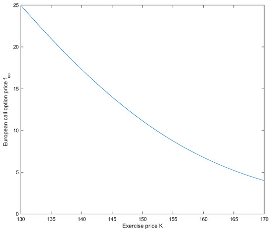
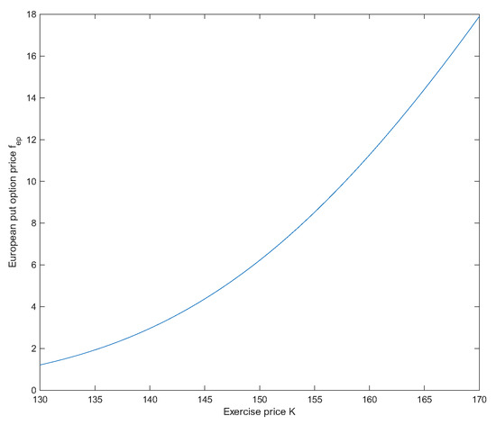
Assume that $m=40,a=0.2,\sigma =0.1$, and $r=0.03$ in the uncertain mean-reverting stock model (1), and $Y_0=130,K=150$, and $s=2$ for European options. Then the prices of European options are $f_{ec}=11.1607$ and $f_{ep}=6.2215$. See Figure 1 and Figure 2.

Example 2.

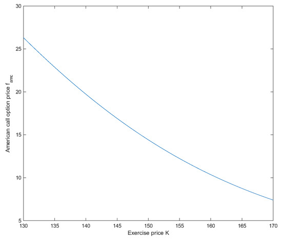
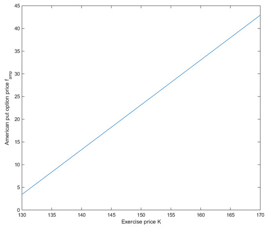
Assume that $m=45,a=0.25,\sigma =0.15$, and $r=0.03$ in the uncertain mean-reverting stock model (1), and $Y_0=130,K=150$, and $s=2$ for American options. Then the prices of American options are $f_{amc}=14.4098$ and $f_{amp}=23.1694$. See Figure 3 and Figure 4.

Example 3.

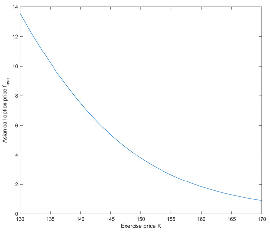
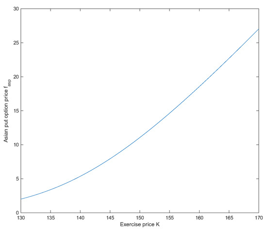
Assume that $m=45,a=0.25,\sigma =0.15$, and $r=0.03$ in the uncertain mean-reverting stock model (1), and $Y_0=130,K=150$, and $s=2$ for Asian options. Then the prices of Asian options are $f_{asc}=3.7888$ and $f_{asp}=11.0602$. See Figure 5 and Figure 6.

Example 4.

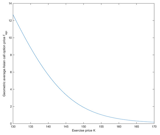
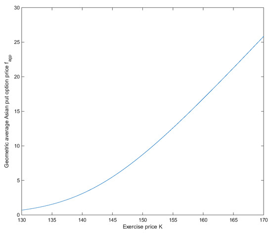
Assume that $m=40,a=0.2,\sigma =0.1$, and $r=0.03$ in the uncertain mean-reverting stock model (1), and $Y_0=130,K=150$, and $s=2$ for geometric average Asian options. Then the prices of geometric average Asian options are $f_{agc}=1.9003$ and $f_{agp}=8.7437$. See Figure 7 and Figure 8.

The numerical results highlight key differences and similarities among the four option types under the mean-reverting stock model. European options serve as the baseline, with their value solely determined by the terminal stock price distribution. American options command a premium due to the early exercise feature, and our model allows for the precise calculation of this premium, which is influenced by the mean-reverting drift. Asian options, by averaging the asset path, exhibit lower volatility and hence a lower premium compared to their European counterparts, a smoothing effect that is particularly valuable for risk-averse investors. Geometric Asian options further enhance this smoothing property due to the nature of geometric averaging. Investors can utilize these models to understand how mean reversion affects the value and optimal exercise strategy of different derivatives, leading to more informed hedging and speculation decisions.

5. Conclusions

This paper derives explicit option pricing formulas under the uncertain mean-reverting stock model, with a special emphasis on the symmetric features embedded in the model and its solutions. The symmetry between call and put options, the time-integral symmetry in Asian options, and the logarithmic symmetry in geometric average options all illustrate how symmetry principles can simplify and unify derivative pricing in uncertain markets. Based on our findings, we recommend that investors and financial analysts consider the mean-reverting property and the inherent symmetries when valuing derivatives in markets exhibiting such characteristics. For future research, several directions emerge: firstly, the symmetry analysis presented here could be extended to more complex exotic options, such as barrier or lookback options. Secondly, while this paper focuses on theoretical derivation, the empirical calibration of the model parameters to market data presents a valuable avenue for further validation and application. Finally, exploring multi-asset options under a correlated uncertain mean-reverting framework would be a natural and challenging extension.

References

- Liu, B. Uncertainty Theory, 2nd ed.; Springer: Berlin/Heidelberg, Germany, 2007. [Google Scholar]
- Liu, B. Toward uncertain finance theory. J. Uncertain. Anal. Appl. 2013, 1, 1. [Google Scholar] [CrossRef]
- Liu, Y.; Liu, B. Residual analysis and parameter estimation of uncertain differential equations. Fuzzy Optim. Decis. Mak. 2022, 21, 513–530. [Google Scholar] [CrossRef]
- Liu, Y.; Liu, B. Estimation of uncertainty distribution function by the principle of least squares. Commun. Stat. Theory Methods 2024, 53, 7624–7641. [Google Scholar] [CrossRef]
- Yang, X.; Ke, H. Uncertain interest rate model for Shanghai interbank offered rate and pricing of American swaption. Fuzzy Optim. Decis. Mak. 2023, 22, 447–462. [Google Scholar] [CrossRef]
- Ye, T.; Liu, B. Uncertain hypothesis test for uncertain differential equations. Fuzzy Optim. Decis. Mak. 2023, 22, 195–221. [Google Scholar] [CrossRef]
- Yang, X.; Li, H. Uncertain finance: A systematic review of recent advances. Fuzzy Optim. Decis. Mak. 2025, 24, 531–561. [Google Scholar] [CrossRef]
- Peng, J.; Yao, K. A new option pricing model for stocks in uncertainty markets. Int. J. Oper. Res. 2011, 8, 18–26. [Google Scholar]
- Tian, M.; Yang, X.; Zhang, Y. Barrier option pricing of mean-reverting stock model in uncertain environment. Math. Comput. Simul. 2019, 166, 126–143. [Google Scholar] [CrossRef]
- Tian, M.; Yang, X.; Zhang, Y. Lookback option pricing problem of mean-reverting stock model in uncertain environment. J. Ind. Manag. Optim. 2021, 17, 2703–2714. [Google Scholar] [CrossRef]
- Liu, B. Some research problems in uncertainty theory. J. Uncertain Syst. 2009, 3, 3–10. [Google Scholar]
- Chen, X. American option pricing formula for uncertain financial market. Int. J. Oper. Res. 2011, 8, 32–37. [Google Scholar]
- Sun, J.; Chen, X. Asian option pricing formula for uncertain financial market. J. Uncertain. Anal. Appl. 2015, 3, 11. [Google Scholar] [CrossRef]
- Zhang, Z.; Liu, W. Geometric average Asian option pricing for uncertain financial market. J. Uncertain Syst. 2014, 8, 317–320. [Google Scholar]
- Cao, J. The pricing of vulnerable options for uncertain financial market. Inf. Int. Interdiscip. J. 2013, 16, 841–846. [Google Scholar]
- Yao, K.; Qin, Z. Barrier option pricing formulas of an uncertain stock model. Fuzzy Optim. Decis. Mak. 2021, 20, 81–100. [Google Scholar] [CrossRef]
- Zhang, Z.; Liu, W.; Sheng, Y. Valuation of power option for uncertain financial market. Appl. Math. Comput. 2016, 286, 257–264. [Google Scholar] [CrossRef]
- Zhang, Z.; Ke, H.; Liu, W. Lookback options pricing for uncertain financial market. Soft Comput. 2019, 23, 5537–5546. [Google Scholar] [CrossRef]
- Yang, X.; Zhang, Z.; Gao, X. Asian-barrier option pricing formulas of uncertain financial market. Chaos Solitons Fractals 2019, 123, 79–86. [Google Scholar] [CrossRef]
- Gao, R.; Liu, K.; Li, Z.; Lv, R. American barrier option pricing formulas for stock model in uncertain environment. IEEE Access 2019, 7, 97846–97856. [Google Scholar] [CrossRef]
- Gao, R.; Wu, W.; Lang, C.; Lang, L. Geometric Asian barrier option pricing formulas of uncertain stock model. Chaos Solitons Fractals 2020, 140, 110178. [Google Scholar] [CrossRef]
- Gao, X.; Jia, L. Pricing formulas of barrier-lookback option in uncertain financial markets. Chaos Solitons Fractals 2021, 147, 110986. [Google Scholar] [CrossRef]
- Pan, Z.; Gao, Y.; Yuan, L. Bermudan options pricing formulas in uncertain financial markets. Chaos Solitons Fractals 2021, 152, 111327. [Google Scholar] [CrossRef]
- Yang, M.; Gao, Y. Pricing formulas of binary options in uncertain financial markets. AIMS Math. 2023, 8, 23336–23351. [Google Scholar] [CrossRef]
- Sun, Y.; Su, T. Mean-reverting stock model with floating interest rate in uncertain environment. Fuzzy Optim. Decis. Mak. 2017, 16, 235–255. [Google Scholar] [CrossRef]
- Sun, Y.; Yao, K.; Dong, J. Asian option pricing problems of uncertain mean-reverting stock model. Soft Comput. 2018, 22, 5583–5592. [Google Scholar] [CrossRef]
- Ji, X.; Zhou, J. Option pricing for an uncertain stock model with jumps. Soft Comput. 2015, 19, 3323–3329. [Google Scholar] [CrossRef]
- Dai, L.; Fu, Z.; Huang, Z. Option pricing formulas for uncertain financial market based on the exponential Ornstein-Uhlenbeck model. J. Intell. Manuf. 2017, 28, 597–604. [Google Scholar] [CrossRef]
- Gao, Y.; Yang, X.; Fu, Z. Lookback option pricing problem of uncertain exponential Ornstein-Uhlenbeck model. Soft Comput. 2018, 22, 5647–5654. [Google Scholar] [CrossRef]
- Liu, Y.; Lio, W. Power option pricing problem of uncertain exponential Ornstein-Uhlenbeck model. Chaos Solitons Fractals 2024, 178, 114293. [Google Scholar] [CrossRef]
- Hassanzadeh, S.; Mehrdoust, F. Valuation of European option under uncertain volatility model. Soft Comput. 2018, 22, 4153–4163. [Google Scholar] [CrossRef]
- Yao, K.; Chen, X. A numerical method for solving uncertain differential equations. J. Intell. Fuzzy Syst. 2013, 25, 825–832. [Google Scholar] [CrossRef]
Disclaimer/Publisher’s Note: The statements, opinions and data contained in all publications are solely those of the individual author(s) and contributor(s) and not of MDPI and/or the editor(s). MDPI and/or the editor(s) disclaim responsibility for any injury to people or property resulting from any ideas, methods, instructions or products referred to in the content. |
© 2025 by the authors. Licensee MDPI, Basel, Switzerland. This article is an open access article distributed under the terms and conditions of the Creative Commons Attribution (CC BY) license (https://creativecommons.org/licenses/by/4.0/).