Intelligent Fault Diagnosis of Rolling Bearings Based on Digital Twin and Multi-Scale CNN-AT-BiGRU Model

Abstract

Rolling bearings constitute critical rotating components within rolling mill equipment. Production efficiency and the operational safety of the whole mechanical system are directly governed by their operational health state. To address the dual challenges of the over-reliance of conventional diagnostic methods on expert experience and the scarcity of fault samples in industrial scenarios, we propose a virtual–physical data fusion-optimized intelligent fault diagnosis framework. Initially, a dynamics-based digital twin model for rolling bearings is developed by leveraging their geometric symmetry. It is capable of generating comprehensive fault datasets through parametric adjustments of bearing dimensions and operational environments in virtual space. Subsequently, a symmetry-informed architecture is constructed, which integrates multi-scale convolutional neural networks with attention mechanisms and bidirectional gated recurrent units (MCNN-AT-BiGRU). This architecture enables spatiotemporal feature extraction and enhances critical fault characteristics. The experimental results demonstrate 99.5% fault identification accuracy under single operating conditions. It maintains stable performance under low SNR conditions. Furthermore, the framework exhibits superior generalization capability and transferability across the different bearing types.

1. Introduction

Under the strategic imperative of high-quality industrial development, rotating machinery serves as critical equipment in industrial systems. They operate in complex environments characterized by high temperatures, fatigue, and heavy-load conditions [1]. Rolling mills represent rotating mechanical equipment for metal processing, inducing the plastic deformation of materials through rolling pressure to modify their geometric configurations and properties [2]. The system comprises multiple components, including frames, work rolls, and transmission mechanisms, with work rolls constituting the core working elements. In the rolling process, work rolls typically need to be supported and rotated by rolling bearings, which make contact with the surface of metal materials to generate frictional forces and compressive stresses. The rolling elements of a bearing are typically distributed in a strictly symmetrical and equidistant manner around the circumference. This rotationally symmetric geometry forms the foundation for stable operation. However, when a pit or spall appears at a specific location on the inner race, outer race, or rolling elements, it fundamentally compromises this structural symmetry. This defect thereby becomes a fixed and asymmetric excitation source, generating abnormal vibration impacts. Rolling bearings endure severe operational environments with continuous heavy-load operation, resulting in frequent failures. Rolling bearing failures critically degrade the stability of rolling mills, potentially triggering catastrophic accidents with substantial economic loss and safety hazards. Fault diagnosis focuses on analyzing a system’s current state by detecting existing anomalies, identifying their specific modes, and isolating faulty components. In contrast, fault prognosis targets the future progression of faults by predicting how anomalies will evolve and estimating components’ remaining useful life. Therefore, health monitoring and fault diagnosis strategies for rolling bearings have become critical for rolling mill maintenance [3].

Fault diagnosis is a key technology to ensure the safe and reliable operation of industrial systems. Its core lies in comprehensively perceiving the abnormal states of the system, determining fault types, and achieving accurate localization by analyzing operational data. A complete diagnostic process starts with fault detection to perceive system anomalies. Then it proceeds to fault identification to determine its specific mode. And finally, it realizes fault isolation to locate the specific component. Brahmbhatt et al. [4] developed a graph-based neural network integrated with system knowledge graphs. By applying advanced graph neural networks, their method significantly enhances fault detection and diagnosis in industrial processes. Gajjar et al. [5] created an integrated framework that combines a neural network classifier with a model-based feedback controller. This hybrid strategy addresses the challenge of concurrent multi-sensor fault detection and system stability control in nonlinear systems. Shahnazari [6] proposed a generic FDI (fault detection and isolation) framework that utilizes specifically designed residual sets. This framework leverages the generated fault signatures to isolate concurrent faults in complex systems without relying on precise models or historical fault data. Xie et al. [7] introduced a digital twin-based approach to tackle issues of redundant data dimensions and high computational load in smart buildings. They employed HVAC system fault detection and diagnosis as a case study to automatically identify and filter critical fault-related data. Consequently, recent advances in the field of fault diagnosis are increasingly integrating digital twins and deep learning to address real-world complexity. These research efforts substantiate the broad applicability of such integrated methodologies across various scenarios. This connectivity links our research on bearing fault diagnosis to the wider domain of engineering fault diagnosis.

Advancements in IoT and AI technologies have propelled intelligent diagnostic methods into research prominence [8]. Vibration signal acquisition from operational rolling bearings enables data-driven fault diagnosis, which typically involves feature extraction [9] and fault classification [10] procedures. Conventional approaches calculate expert-defined fault features for classification using shallow machine learning models, such as support vector machines [11,12,13], random forests [14,15], and decision trees [16,17]. Despite demonstrating their efficacy in early stage applications, these methods have exhibited critical limitations. An overreliance on domain expertise impedes a model’s self-adaptation capabilities. In addition, shallow architectures fail to capture the complex nonlinear features in operational processes.

Deep learning (DL) methods have distinct advantages over conventional diagnostic techniques for fault-identification applications. This approach autonomously learns feature representations from raw vibration signals, eliminating expert dependency while addressing diagnostic challenges under complex working conditions. Cui et al. [18] developed a residual network integrated with Singular Value Decomposition (SVD), employing SVD pooling layers for signal denoising before feeding wavelet time–frequency maps into an enhanced ResNet architecture for fault classification. However, this method suffers from excessive computational complexity, which significantly compromises model training efficiency. Zhang et al. [19] presented a DL model in response to the complex fault types encountered in industrial wind turbines. This approach transforms one-dimensional vibration data into two-dimensional image to enhance feature representation and concurrently redesigns the deep residual network architecture to optimize kernel sensitivity. This study provides a novel framework for fault diagnosis in complex industrial data environments. Zhu et al. [20] innovatively employed a wide-kernel convolutional structure to eliminate high-frequency noise interference in vibration signals, substantially improving the diagnostic performance by expanding the size of the convolutional kernels. Chen et al. [21] designed a neural network that automatically learns features. This technique uses dual-branch convolutional neural networks with different kernel sizes to automatically extract multi-frequency characteristics after directly processing raw vibration signals as input. These features are subsequently input into LSTM network for fault type classification. This method offers a new avenue for the diagnosis of intelligent bearing faults.

DL based data-driven fault diagnosis methods require the prior acquisition of complete fault pattern datasets for model training [22,23]. However, such datasets are often unavailable in critical industrial scenarios, fundamentally limiting the applicability of data-driven approaches. Digital twin (DT) technology has emerged as an emerging technology that addresses the scarcity of training data in mechanical health management through virtual–physical interaction [24]. DT serves as a virtual representation of a physical system. It employs digital methods to construct a dynamic model that captures multi-dimensional, multi-spatiotemporal scale, and multi-physical quantity characteristics. This model simulates the attributes, behaviors, and principles of the physical entity in real-world environments. It can be utilized to generate high-fidelity simulated data for various engineering applications. Under insufficient fault data conditions, the DT establishes digital models of physical entities to reflect operational states, providing reliable data support for fault diagnosis and prognosis. Xia et al. [25] proposed a DT-assisted triplex pump diagnostic method that employs simulated fault data from digital models and implements fault identification through sparse denoising autoencoder networks. Yan et al. [26] proposed a DT-enhanced imbalanced fault diagnosis framework that generates simulated data through gearbox nonlinear dynamic analysis and digital twin modeling to overcome the difficulty in acquiring actual fault data. Zhang et al. [27] created a dynamic DT-bearing model to simulate operational conditions and generate sufficient fault datasets to resolve diagnostic challenges using unlabeled health status data. Li et al. [28] devised a DT-based synthetic data augmentation method using DT models to generate simulated data, coupled with a lightweight CNN architecture integrating focal modulation mechanisms (FM-LCN) to enhance the diagnostic accuracy. Ming et al. [29] designed a DT-assisted diagnostic framework combining frequency-domain filtering and subdomain adaptation networks to achieve cross-condition feature space alignment, significantly improving the performance under data imbalance.

While DL and DT applications have been separately investigated for bearing fault diagnosis, an integrated framework is notably absent. Inspired by the existing literature, this study proposes an innovative methodology integrating DT technology with the multi-scale convolutional neural network with attention mechanisms and bidirectional gated recurrent unit (MCNN-AT-BiGRU) hybrid diagnostic model for rolling bearing fault diagnosis. First, a rolling bearing DT model for rolling bearings is established by leveraging the geometric symmetry of rolling bearings to simulate multiple failure modes and their evolutionary processes. The model generates simulated data, which is subsequently infused into actual datasets via a hierarchical hybrid strategy to balance the distribution of fault categories. The MCNN-AT-BiGRU hybrid diagnostic model with a symmetric network structure is then constructed. This model makes use of a symmetrically parallel convolutional neural network layer structure for multi-scale feature extraction, while employing an attention mechanism to accurately capture key features in fault signals. These key features often manifest as asymmetric transient impulses. Furthermore, the deep focus on and fusion of these asymmetric features serve as the key to the model achieving high-precision fault diagnosis. By capturing the bearing fault periodicity characteristics, the bidirectional gated recurrent units architecture extracts temporal features from the vibration signals to achieve spatiotemporal feature integration. The principal contributions of this work are as follows:

(1)

To overcome the limitations of purely data-driven methods, this study develops a DT framework. The framework is centered on a high-fidelity model of rolling bearings. It incorporates the physical dimensions of the bearing and physical principles. The model generates diverse types of physics-consistent fault simulation data. This capability effectively addresses the challenge of data scarcity.

(2)

The symmetric network architecture of MCNN-AT-BiGRU is developed, optimizing parameters through virtual–real data co-training and innovatively integrating multi-scale convolutional neural networks (MCNNs) with bidirectional gated recurrent units (BiGRUs) for spatiotemporal complementary feature representation. By leveraging the physical characteristics of bearing faults, the attention mechanism (AT) is incorporated to precisely capture asymmetric transient impulses within fault signals. The deep focus on and fusion of these asymmetric features enhance the model’s accuracy in identifying fault types.

(3)

The experimental results establish the greater recognition accuracy of the proposed method over mainstream diagnostic models in noisy environments and varying operational conditions. Meanwhile, the proposed method maintains stable performance in cross-bearing-type transfer experiments. These results indicate the robustness of the model in mitigating noise interference and adapting to complex industrial settings, exhibiting exceptional generalization performance and transferability.

Section 2 details the DT model for rolling bearings. Section 3 describes the architecture of the proposed hybrid diagnostic model composed of a multi-scale convolutional neural network with an attention mechanism and a bidirectional gated recurrent unit (MCNN-AT-BiGRU), along with the integrated fault diagnosis process. Section 4 presents the experimentally designed scenarios to validate and discuss the performance of the MCNN-AT-BiGRU model. Section 5 concludes the study and outlines prospective research directions.

2. Digital Twin Model of Rolling Bearing

DT technology tightly integrates advanced information technology with digital modeling methods. Through the interaction between physical objects and their virtual representations, it can meticulously depict the multi-dimensional characteristics, behaviors, and current states of objects. Unlike fault state observers, which are typically designed for real-time state estimation and residual generation within a specific operational mode, DT places greater emphasis on constructing a dynamic model that fully corresponds to the physical entity. Given that vibration signals are commonly utilized as monitoring data reflecting mechanical health, dynamic models have become the core module for realizing equipment condition perception by accurately simulating the vibration characteristics of the system. DT models constructed based on dynamic simulations can mirror the real-time operational status of rolling bearings. By generating fault data that covers multiple operating conditions, they can accurately simulate the dynamic characteristics of bearings under normal operation and under various failure modes, namely outer ring faults, inner ring faults, and roller faults.

2.1. Construction of Digital Twin Model

This study employs a lumped-mass approach to model rolling bearing dynamics. The model neglects raceway waviness and rotational inertia to obtain the dynamic response characteristics [30]. Dynamic methods start from the perspective of vibration generation mechanisms. Based on Newton’s second law, theoretical models are built via mathematical formulation. A five-degree-of-freedom vibration model was adopted for rolling bearings in this paper. It comprised four degrees of freedom associated with the horizontal and vertical motions of the inner and outer rings, with the remaining one corresponding to a unit resonator. The structural diagram is shown in Figure 1. Four spring–damper systems connected the inner and outer rings. Another spring–damper system represented the unit resonator.

The dynamic differential equations of the model are as follows:

$$\left\{\begin{array}{c}{F}_x-K_P{x}_o-R_P{\dot{x}}_o-M_P{\ddot{x}}_o=0\hfill \\ F_y-M_{P}G-(R_P+R_R){\dot{y}}_o-(K_P+K_R)y_o+K_R{y}_R+R_R{\dot{y}}_R-M_P{\ddot{y}}_o=0\hfill \\ K_R(y_o-y_R)+R_R({\dot{y}}_o-{\dot{y}}_R)-M_R{\ddot{y}}_R-M_{R}G=0\hfill \\ F_x-K_S{x}_i-R_S{\dot{x}}_i+M_S{\ddot{x}}_i=0\hfill \\ F_y+M_{S}G+K_S{y}_i+R_S{\dot{y}}_i+M_S{\ddot{y}}_i=0\hfill \end{array}\right.$$

(1)

where $M_S$, $M_P$, and $M_R$ represent the masses of the inner ring, outer ring, and unit resonator. $R_S$, $R_P$, and $R_R$ denote the damping values of the inner ring, outer ring, and unit resonator. $K_S$, $K_P$, and $K_R$ stand for the stiffness values of the inner ring, outer ring, and unit resonator. $x_i$, $y_i$, $x_o$, and $y_o$ are the horizontal and vertical displacements of the inner and outer rings’ center of mass. G is the the gravitational acceleration.

The azimuth angle ${\varphi }_j$ of the roller can be determined by the following:

$${\varphi }_j={\displaystyle \frac{2\pi (j-1)}{N_b}}+{\omega }_{c}t+{\varphi }_0$$

(2)

where $N_b$ denotes the total number of rollers, ${\varphi }_0$ is the initial azimuth angle of the first roller, j is an integer from 1 to $N_b$, and ${\omega }_c$ is the rotational angular velocity of the cage, which can be derived from the angular velocity ${\omega }_s$ of the drive shaft linked to the inner ring.

$${\omega }_c=\left(1-{\displaystyle \frac{d}{D}}\right){\displaystyle \frac{{\omega }_s}{2}}$$

(3)

where D and d represent the bearing pitch diameter and roller diameter.

Based on the vibration mechanism of bearings, the Hertzian contact theory was employed to calculate the contact forces between the rollers and the rings of the bearing. The corresponding formula is presented as follows:

$$f_j=K_b·{\delta }_j^{3/2}$$

(4)

where ${\delta }_j$ represents the deformation of the $j\mathrm{th}$ roller, $K_b$ denotes the stiffness coefficient of the roller, and $f_j$ is the contact force between the $j\mathrm{th}$ roller and the ring.

$${\delta }_j=x_{d}cos{\varphi }_j+y_{d}sin{\varphi }_j-{\delta }_c$$

(5)

where $x_d$ and $y_d$ indicate the relative displacements of the roller in the horizontal and vertical directions, ${\varphi }_j$ is the angular position of the $j\mathrm{th}$ roller, and ${\delta }_c$ represents the radial clearance.

According to Equations (2)–(5), the contact force of each roller can be obtained. By decomposing this contact force into horizontal and vertical directions through angular relationships, it can be derived that

$$\left\{\begin{array}{c}{F}_x={\displaystyle \sum _{j=1}^{N_b}}{f}_{j}cos{\varphi }_j·H\left({\delta }_j\right)\hfill \\ F_y={\displaystyle \sum _{j=1}^{N_b}}{f}_{j}sin{\varphi }_j·H\left({\delta }_j\right)\hfill \end{array}\right.$$

(6)

The predicted contact force $f_j$ between the roller and the ring becomes negative when the deformation ${\delta }_j$ is negative. In reality, no contact occurs in this case. Therefore, negative contact force values are discarded by defining $H\left({\delta }_j\right)$, and the contact force of the $j\mathrm{th}$ roller is only considered when the deformation is positive, expressed as follows:

$$H\left({\delta }_j\right)=\left\{\begin{array}{cc}1,\hfill & \mathrm{if}{\delta }_j>0\\ 0,\hfill & \mathrm{if}{\delta }_j\le 0\end{array}\right.$$

(7)

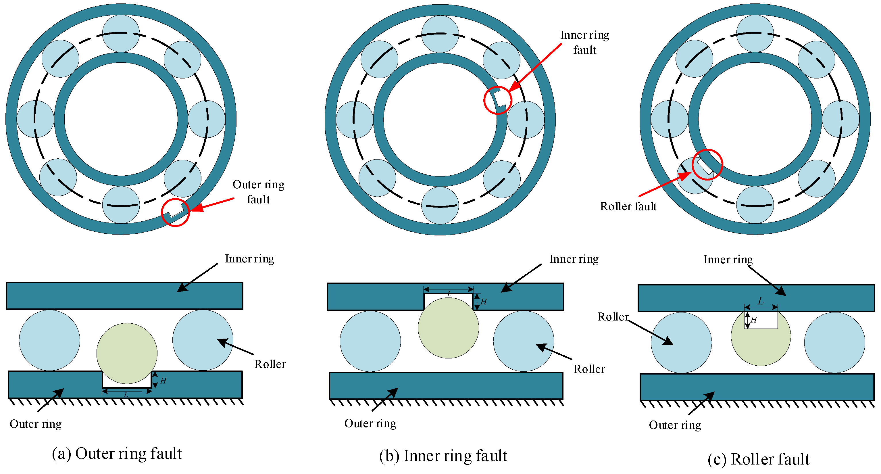
The developed dynamic simulation model analyzed three typical failure modes in rolling bearings: outer ring, inner ring, and roller faults. The occurrence of local defect faults destroys the inherent geometric symmetry of the bearing, thereby impairing its dynamic characteristics required for stable operation. Characteristic periodic impact vibration responses are generated when the roller traversed the damaged zone. As shown in Figure 2, to develop a generalized dynamic model applicable to various damage patterns, local defects are modeled as rectangular spalls geometrically simplified into raceway pits, where H denotes the defect depth and L represents the defect length. The rollers are assumed not to contact the bottom of the defect, and the defect is simplified as a rectangle extending across the entire width of the raceway. This assumption allows the model to bypass complexities arising from irregular geometrical details, thereby focusing on the fundamental periodic impulse response triggered by the presence of the damage itself.

As shown in Figure 2a, when a defect occurs on the outer ring, the contact force will suddenly disappear as the roller enters the spall zone, and will recover when it leaves the spall zone. These contact losses and contact gains lead to the generation of a large number of periodic impulsive forces. At this time, the contact deformation under the outer ring fault is as follows:

$${\delta }_o={\displaystyle \frac{d}{2}}-\sqrt{{\left({\displaystyle \frac{d}{2}}\right)}^2-{\left({\displaystyle \frac{L_o}{2}}\right)}^2}$$

(8)

where d denotes the diameter of the roller.

When the roller passes through the defective area of the outer ring, the deformation generated will change compared with that when passing through the defect-free area, and the total deformation is ass follows:

$${\delta }_j=x_{d}cos{\varphi }_j+y_{d}sin{\varphi }_j-{\delta }_o-{\delta }_c$$

(9)

As shown in Figure 2b, when a defect occurs on the inner ring, its modeling method is similar to that of the above-mentioned outer ring defect. The contact deformation under the inner ring fault is as follows:

$${\delta }_i={\displaystyle \frac{d}{2}}-\sqrt{{\left({\displaystyle \frac{d}{2}}\right)}^2-{\left({\displaystyle \frac{L_i}{2}}\right)}^2}$$

(10)

When the roller passes through the defective area of the inner ring, the total deformation is as follows:

$${\delta }_j=x_{d}cos{\varphi }_j+y_{d}sin{\varphi }_j-{\delta }_i-{\delta }_c$$

(11)

As shown in Figure 2c, when a defect occurs in the roller, the crack rotates with the roller and makes contact with the inner and outer rings. The contact deformation loss caused by this interaction can be determined using the following calculation:

$${\delta }_b={\displaystyle \frac{d}{2}}-\sqrt{{\left({\displaystyle \frac{d}{2}}\right)}^2-{\left({\displaystyle \frac{L_b}{2}}\right)}^2}$$

(12)

Based on the previously determined contact deformation loss, it can be inferred that the total deformation occurs when the roller defect makes contact with either the inner or outer ring. The total deformation is as follows:

$${\delta }_j=x_{d}cos{\varphi }_j+y_{d}sin{\varphi }_j-{\delta }_b-{\delta }_c$$

(13)

Finally, the vibration response of the bearing is obtained by solving Equation (1) using the fourth-order fixed-step Runge–Kutta method. We used a fixed time step of $8.33\times {10}^{-5}$ s (12 kHz sampling).

2.2. Validation of Digital Twin Model

A visual comparison between the simulated and corresponding measured signals was performed in order to verify the accuracy of the digital twin model. When the rolling bearing fails, repeated impacts between the roller and ring induce periodic low-frequency vibrations, which are the characteristic frequencies exhibited during bearing faults. The characteristic frequencies of rolling bearings are determined by geometric parameters, and they are as follows:

$${\mathrm{BPF}}_{\mathrm{O}}={\displaystyle \frac{N_{\mathrm{b}}{f}_{\mathrm{s}}}{2}}\left(1-{\displaystyle \frac{d}{D}}\right)$$

(14)

$${\mathrm{BPF}}_{\mathrm{I}}={\displaystyle \frac{N_{\mathrm{b}}{f}_{\mathrm{s}}}{2}}\left(1+{\displaystyle \frac{d}{D}}\right)$$

(15)

$${\mathrm{BPF}}_{\mathrm{B}}={\displaystyle \frac{N_{\mathrm{b}}{f}_{\mathrm{s}}}{2}}\left(1-{\displaystyle \frac{d^2}{D^2}}\right)$$

(16)

where ${\mathrm{BPF}}_{\mathrm{O}}$ is the fault frequency associated with the outer ring of the bearing, ${\mathrm{BPF}}_{\mathrm{I}}$ denotes the fault frequency associated with the inner ring of the bearing, ${\mathrm{BPF}}_{\mathrm{B}}$ corresponds to the fault frequency associated with the rollers of the bearing, and $N_b$ represents number of rollers, $f_r$ is the bearing rotational frequency.

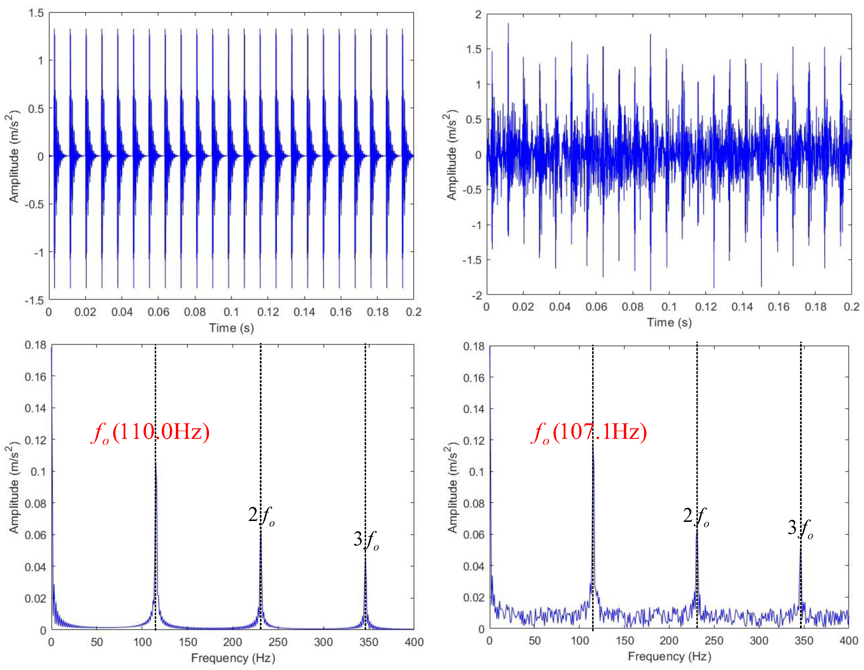
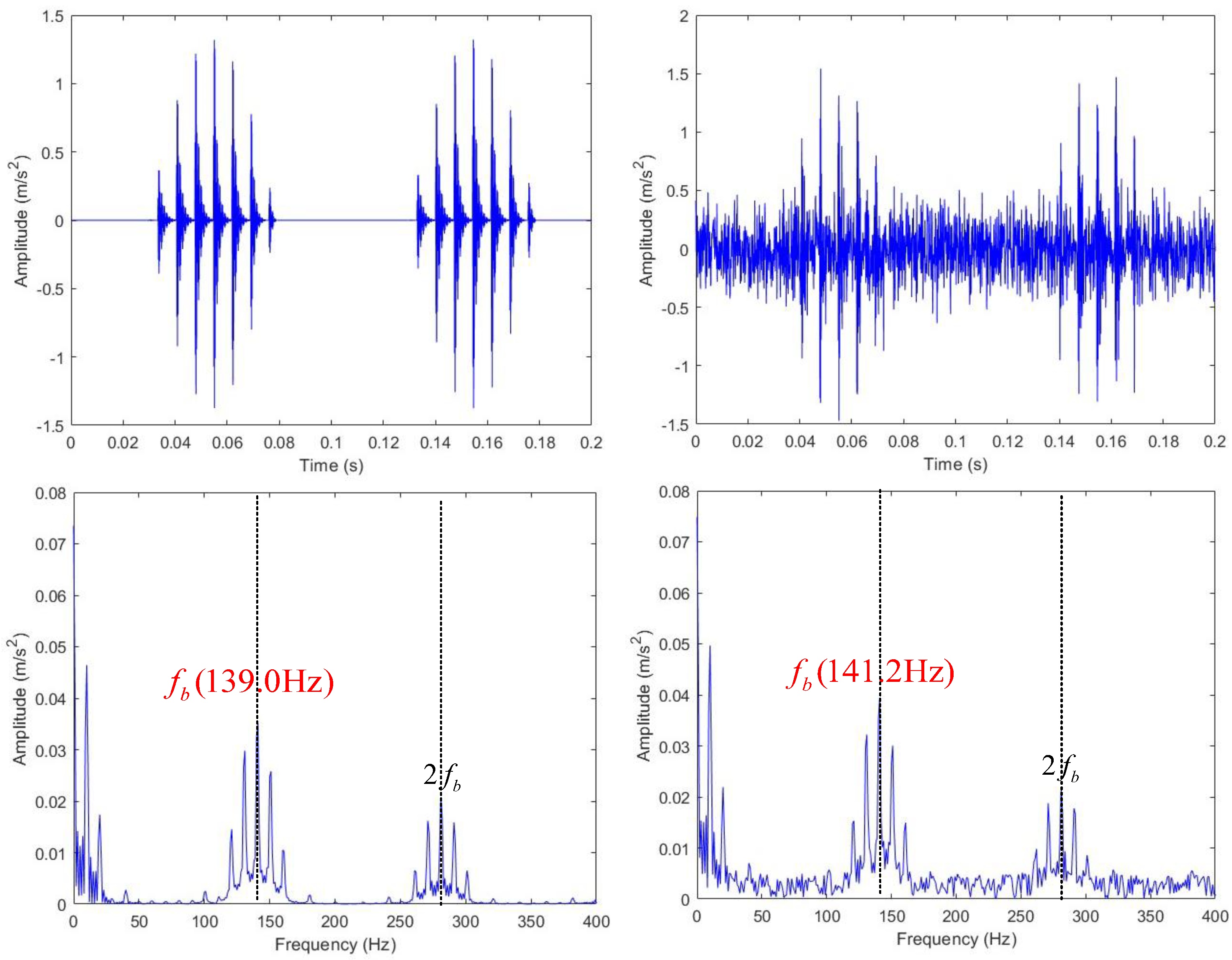
The simulation model employed the bearing type and geometric parameters given in

Table 1. Geometric parameters of SKF6205 bearing.

Parameter	Value
Diameter of outer ring ($D_o/\mathrm{mm}$)	52
Diameter of inner ring ($D_i/\mathrm{mm}$)	25
Radial internal clearance (${\delta }_c/\mathsf{\mu }\mathrm{m}$)	13
Diameter of roller center circle ($d/\mathrm{mm}$)	7.94
Diameter of pitch ($D/\mathrm{mm}$)	39.04
Number of rollers ($N_b$)	9

. When the bearing operated at a rotational speed of 1797 revolutions per minute, the corresponding rotational frequency was 29.95 Hz. Using Equations (14)–(16), the computed characteristic frequencies for roller, inner ring, and outer ring damage were 141.17 Hz, 162.19 Hz, and 107.36 Hz. An envelope spectrum analysis was performed on the simulated inner ring, outer ring, and roller faults of the bearing.

As shown in Figure 3, Figure 4 and Figure 5, the envelope spectrum analysis of the simulated signals revealed distinct fault characteristics. The detected fault frequencies for the outer ring, inner ring, and roller faults were 110 Hz, 169 Hz, and 139 Hz, respectively. When calculating the error for the fault frequency identified via the envelope spectrum analysis, this error is a static relative error derived from the comparison between the theoretically calculated value and the peak frequency in the envelope spectrum. These values correspond closely to the theoretical fault frequencies, with relative theoretical ${\mathrm{BPF}}_{\mathrm{O}}$/${\mathrm{BPF}}_{\mathrm{I}}$/${\mathrm{BPF}}_{\mathrm{B}}$ errors of only 2.7%, 1.4%, and 1.5%. Furthermore, the spectra exhibited prominent peaks at twice and three times the fundamental fault frequencies, forming clear harmonic families. The presence of such pronounced peaks, particularly with harmonic repetitions, indicates the existence of localized faults. The combination of accurate frequency matching and identifiable harmonic structures confirms that the fault simulation accuracy of the model is in good agreement with real-world bearing fault manifestations.

To further validate the generalization capability of the proposed DT model, we conducted additional validation through envelope spectrum analysis across different rotational speeds. By performing this analysis on simulated vibration signals under various fault locations and rotational speeds, the fundamental frequency peaks were extracted and compared against the theoretical fault characteristic frequencies calculated from the formulas. As shown in

Table 2. Relative error of the fundamental frequency under different rotational speeds.

Fault Location	Rotational Speed
	1730 (r/min)	1750 (r/min)	1772 (r/min)	1797 (r/min)
Outer ring	2.2%	2.9%	2.5%	2.7%
Inner ring	1.7%	1.2%	1.6%	1.4%
Roller	1.9%	2.1%	1.8%	1.5%

, the relative error of the fundamental frequency remained below 3% under all the tested rotational speed conditions.

These findings prove validity and utility of the proposed DT model for rolling bearing fault simulation. The established rolling bearing dynamic model enables the systematic acquisition of physical characteristics across diverse fault conditions.

3. Overview of the Proposed Fault Diagnosis Framework

Figure 6 illustrates the proposed overall fault diagnosis framework. This framework synergistically combines DT and DL technologies to optimize model performance through augmented datasets to enable online diagnosis and dynamic adaptation in industrial settings. The diagnostic workflow is divided into five stages: signal acquisition, signal preprocessing, offline training, online testing, and industrial deployment. The detailed diagnostic procedures are as follows:

(1)

Signal acquisition: The actual vibration signals of the physical bearings are gathered using sensors. A DT bearing model is established based on the geometric dimensions of rolling bearings to simulate multiple fault modes and generate simulation data. A hierarchical hybrid strategy is adopted to inject simulated data into the actual dataset at a certain proportion, balancing the class distribution of the fault samples.

(2)

Signal preprocessing: Data segmentation is performed in the form of sliding windows to generate multiple local segments to create a sample dataset. The Z-Score standardization method is used for normalization. The dataset is split into a training set and a test set according to a preassigned proportion, with the former for model parameter tuning and the latter for performance assessment. To prevent data leakage, we adopted a rigorous split-by-source strategy. Specifically, prior to segmenting the data, all samples are grouped according to their original acquisition source. All segments derived from the same original recording are assigned collectively to either the training or test set, thus ensuring no temporal overlap between the two sets.

(3)

Offline training: The MCNN-AT-BiGRU model processes training samples with configured hyperparameters and adaptive learning rates by employing backpropagation for error computation and parameter updates. Training efficiency is enhanced through early stopping mechanisms that monitor convergence patterns during iterative optimization.

(4)

Online testing: The optimized MCNN-AT-BiGRU model receives testing samples from the physical bearing to generate diagnostic results. This is crucial for validating the practical applicability of our model.

(5)

Industrial deployment: The actual operational data collected from industrial sites are input into the pre-trained diagnostic model, and the model performance is optimized and improved through model parameter fine-tuning using transfer learning.

3.1. Proposed MCNN-AT-BiGRU Network Model

3.1.1. Model Description

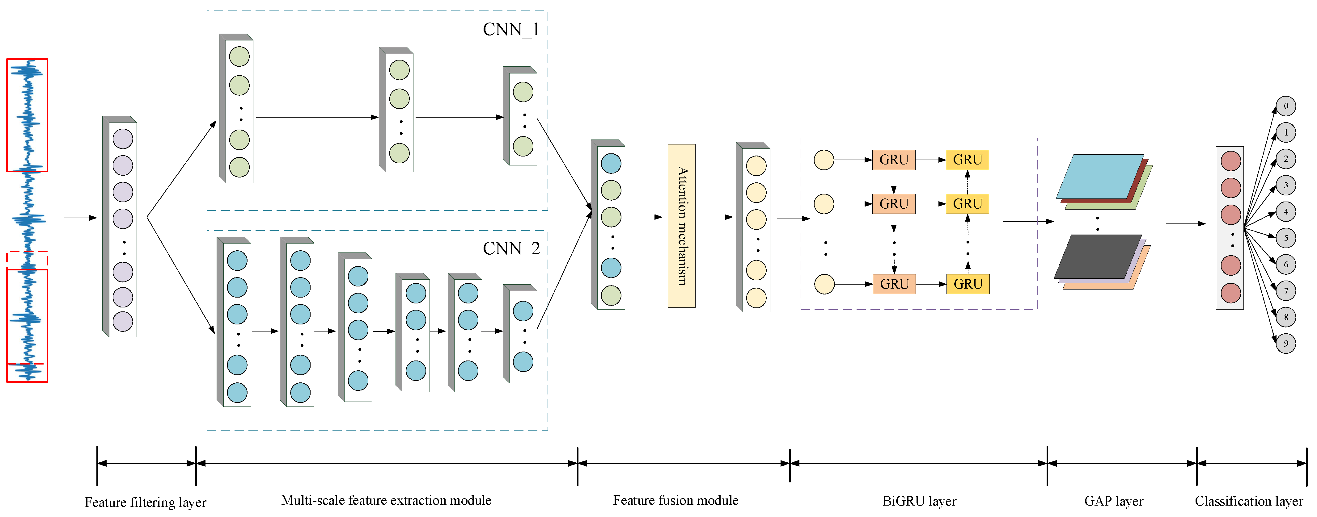
The architecture of the proposed MCNN-AT-BiGRU rolling bearing fault diagnosis model is illustrated in Figure 7. The model applies overlapping sampling processing to the collected vibration signals to generate data samples suitable for deep-learning models. In terms of model structure design, deep spatial features are extracted from time-domain signals through a symmetrically parallel convolutional neural network layer structure. The attention mechanism captures asymmetric transient impulses in fault signals, achieves deep focus on and fusion of these asymmetric features, and dynamically adjusts the weight distribution across feature channels. The BiGRU layer captures the temporal features that undergo dimensionality reduction through global average pooling. Finally, the FC (fully connected) layer outputs the fault diagnosis results.

The feature screening layer of this diagnostic model employs a wide convolutional kernel 64 × 1 with a stride of 16, significantly enhancing the model’s stability under noise interference. Bearing fault features primarily manifest as low-frequency vibration components. Therefore, this wide convolutional kernel structure is characterized by excellent low-frequency feature capture capability. It also maintains fixed stride conditions and suppresses high-frequency noise interference. Additionally, considering the periodic characteristics of bearing vibration signals, enlarging the convolutional kernel size expands the model’s receptive field range, thereby better capturing the global periodic features of signals [31]. Based on the feature-filtered layer, this study further constructs a multi-scale feature extraction architecture. This architecture enhances the representation of fault features across different scales. It achieves this enhancement through the design of parallel and symmetric convolutional pathways. Specifically, CNN_1 employs smaller receptive fields (3 × 1 and 1 × 1) to extract high-frequency features, whereas CNN_2 adopts larger receptive fields (10 × 1 and 6 × 1) to capture the low-frequency signal characteristics.

Global Max Pooling (GMP) provides determinative impulses for the signal feature matrix, which serves as the primary discriminative criteria for fault diagnosis. This attention mechanism employs the GMP to compress the dimensionality of the input feature matrix. This information is then transformed into attention weights via convolutional mapping operations. By applying these attention weights to the initial feature matrix, the model is able to concentrate on the important channel data. The basis for the BiGRU’s future learning of temporal properties is laid by this procedure. Ultimately, global average pooling (GAP) is utilized to reduce the dimensionality of high-dimensional features, and the probability distribution of fault kinds is then computed using the FC layer to produce diagnostic results.

The detailed model parameters are enumerated in

Table 3. Model architecture parameters.

Network Layer	Kernel Size	Stride	Activation Function	Input Dimension	Output Dimension
Input layer	-	-	-	-	$1024\times 1$
Wide-Conv	$64\times 1$	16	Tanh	$1024\times 1$	$64\times 16$
Pooling layer	$2\times 1$	2	-	$64\times 16$	$32\times 16$
CNN_1	$10\times 1$	1	Tanh	$32\times 16$	$32\times 30$
	$6\times 1$	1
CNN_2	$3\times 1$	1	Tanh	$32\times 16$	$32\times 30$
	$1\times 1$	1
Attention layer	1	1	Tanh	$32\times 30$	$32\times 30$
BiGRU	-	-	Tanh	$32\times 30$	$36\times 30$
GAP layer	-	-	-	$36\times 30$	$1\times 30$
FC layer	-	-	Softmax	30	10

. In the proposed MCNN-AT-BiGRU model, Tanh was chosen to serve as the activation function instead of ReLU. In bearing fault diagnosis, the negative values of vibration signals contain crucial phase and impulse response information. The Tanh function preserves this critical information, in contrast to ReLU-based activations, which zero out these negative components. It is noteworthy that each convolutional layer is followed by a batch normalization layer. This design not only accelerates model convergence but mitigates the gradient saturation problem of the Tanh function at extreme input values by standardizing the inputs to the activation function, thereby enhancing the training stability and robustness of the model.

3.1.2. The Proposed Signal Attention Mechanism Module

Coordinate attention is an enhanced attention mechanism, originally applied in image processing tasks, that concurrently captures information across both spatial and channel dimensions. It decomposes the feature map into horizontal and vertical attentions, and then recombines them. In this way, it enhances the information interaction between channels while maintaining position sensitivity [32].

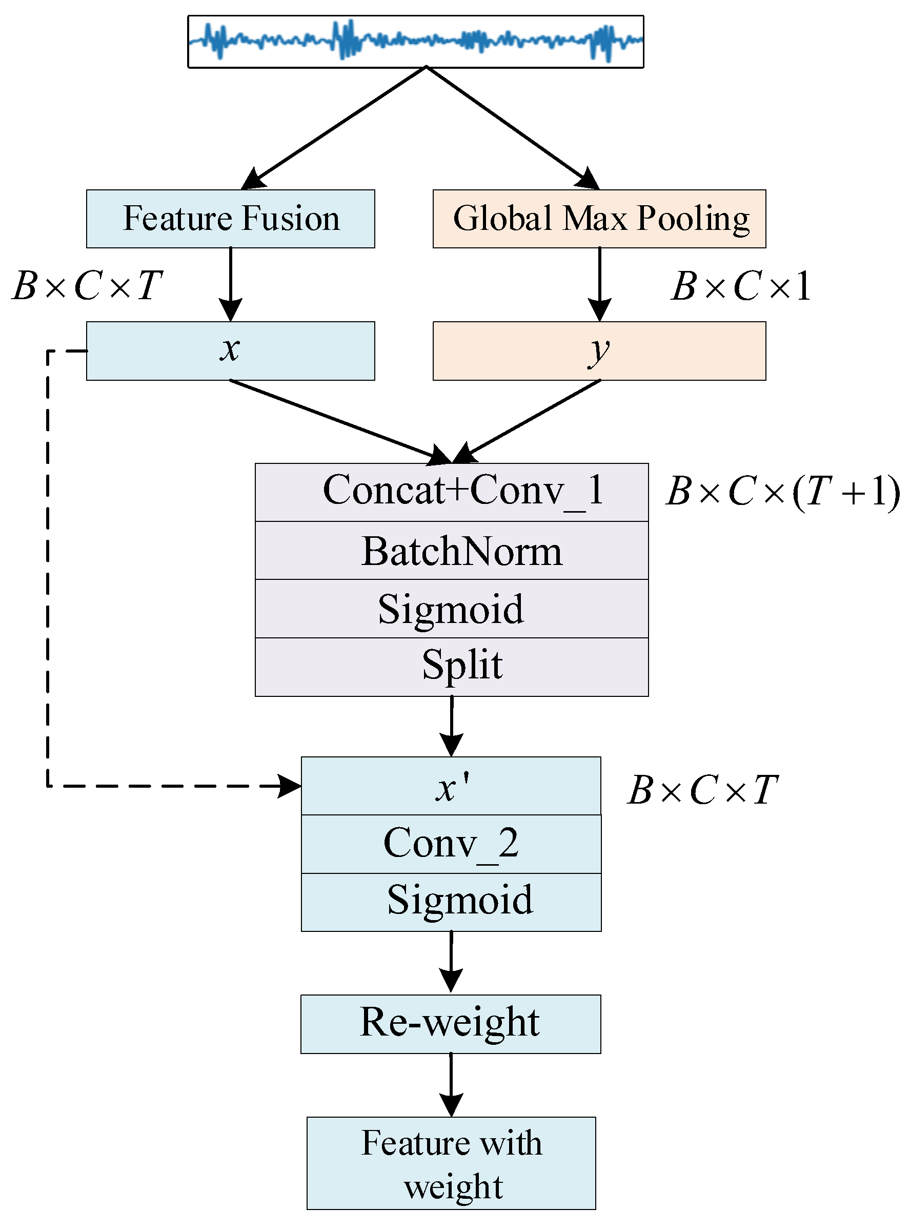
For vibration signals, the structural advantages of coordinate attention can be leveraged to enhance the focus on the pulse occurrence regions along the time axis. Subsequently, the output of this attention mechanism module is element-wise multiplied with the original feature quantities to highlight the features corresponding to fault pulses. The architecture of the proposed signal attention mechanism is shown in Figure 8.

First, GMP is used to generate the key pulse feature y in order to extract pulses in each channel and record the salient characteristics of the signal. Then, the original feature x is integrated with the key pulse feature y. Through convolution mapping of the transitional feature F using the shared convolution kernel $\mathrm{Conv}\_1$, the intermediate feature $F_1$ is generated after normalization and activation.

$$F=\mathrm{Concat}(x,y)$$

(17)

$$F_1=\xi \times \mathrm{BN}\left[\mathrm{Conv}\_1\left(F\right)\right]$$

(18)

where $\mathrm{Concat}$ denotes the concatenation operation of feature matrices, $\mathrm{BN}$ is the normalization layer, and $\xi$ represents the sigmoid activation function.

Next, the intermediate feature $F_1$ is split into two separate tensors. One of the tensors, $x^{\prime }$, is kept to have the same spatial dimensions as before. It is mapped to have the same number of channels the original input x through the convolution kernel $\mathrm{Conv}\_2$ to generate the weight coefficient $F_2$.

$$F_2=\xi \times \mathrm{Conv}\_2(x^{\prime })$$

(19)

Finally, the weight coefficients $F_2$ are multiplied by the original features x channel-wise to obtain the weighted features Z.

$$Z=F_2\otimes x$$

(20)

3.2. Signal Acquisition Module

The signal acquisition module comprises acceleration vibration sensors, a current-regulated adapter, a data acquisition card, and host computer software. During the collection of actual signals, the bearing housing was selected as the sampling position in this study. The vibration of the bearing is mainly transmitted through rigid structures such as the bearing housing and the shell. To minimize the attenuation of vibration signals to the greatest extent, the vibration sensor is fixed on the bearing housing. This position ensures the shortest transmission path of vibration signals from the vibration source to the sensor. It also minimizes energy attenuation, thereby truly reflecting the vibration state of the bearing.

The vibration acquisition system utilizes an IEPE-type accelerometer (Model CT1005LC), which has a built-in charge amplifier that converts the charge signal into a voltage, thereby enhancing anti-interference capability. The constant current adapter (Model CT5204) is equipped with an integrated signal conditioning module that provides a 2 mA constant current source to power the sensor. For data acquisition, the USB-1608G card is selected for its high-precision and high-speed sampling capabilities. The vibration signals are fed into this card differentially, where they are converted from analog to digital form. Finally, the digitized data is transmitted via an interface to the host computer running the DAQami software v4.1, enabling real-time monitoring and acquisition. A flowchart of the entire acquisition module is shown in Figure 9.

In the host computer data analysis DAQami software v4.1 that matches the data acquisition card, parameters such as sampling channels, sampling frequency, and sampling duration can be selected. Observing the real-time data changes on the host computer interface enables a better assessment of the bearing’s operational health. Meanwhile, the collected data can be stored locally, facilitating subsequent analysis and processing of vibration signals.

4. Experiments and Results

In this section, experiments were conducted under four scenarios: single operating conditions, noise interference, variable operating conditions, and cross-bearing generalization performance, with a subsequent analysis to verify the effectiveness of the proposed methodology. The classification accuracy was chosen as the main performance parameter to assess the model’s capacity for diagnosis. All the experiments shared identical runtime environments. The implementation used Python 3.9 and was developed on the PyTorch 2.1 framework. The hardware consisted of an NVIDIA GeForce RTX 4060 GPU and an Intel Core i7-12700H CPU.

4.1. Dataset Description

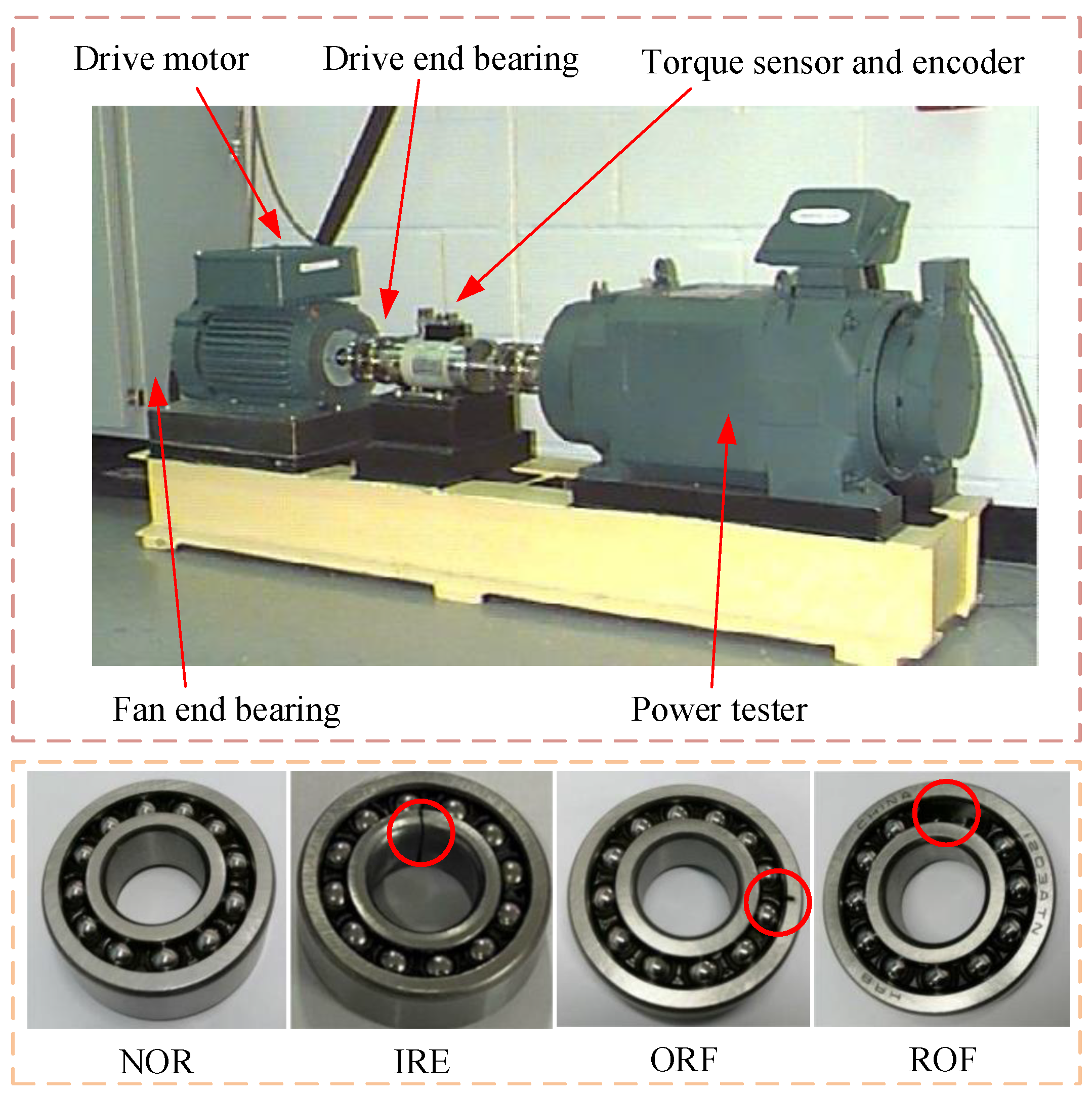
The experimental data in this study originated from the Case Western Reserve University (CWRU) Bearing Data Center [33]. Vibration signals were collected from the drive-end SKF-6205-2RS deep-groove ball bearings using the setup shown in Figure 10. The sampling frequency was set to 12 kHz. The dataset encompassed four operational conditions (0, 1, 2, and 3 hp, where 1 hp = 745.7 W) and ten bearing health states, including NOR (normal state), IRF (inner ring fault), ORF (outer ring fault), and ROF (roller fault), with defect diameters of 0.178 mm, 0.356 mm, and 0.534 mm. All the faults were introduced using EDM (electrical discharge machining), a technique that generates highly precise and controllable pits on metal materials through electrical discharges. Each state comprised 100 samples (1024 points per sample), totaling 1000 samples. To address fault sample scarcity, a bearing dynamics model was constructed using DT technology. This model simulated the operating conditions and fault patterns identical to real data to generate simulated vibration signals. A stratified hybrid strategy involved the injection of synthetic data into a measured dataset. The normal state retained all 100 originally measured samples. Mild wear (0.178 mm) and moderate wear (0.356 mm) mixed 50 measured and 50 simulated samples in a 1:1 ratio. Severe spalling faults (0.534 mm) combined 20 measured and 80 simulated samples at 1:4 ratio, ensuring a total of 100 samples per health state. The final augmented datasets A/B/C/D (corresponding to the four operating conditions) preserved 1000 total samples, divided into a training set (700 samples) and a test set (300 samples) at a 7:3 ratio. The test set exclusively contained unreplaced original measured data to validate model generalization. The dataset configurations are listed in

Table 4. CWRU bearing augmented dataset.

Bearing Condition	Fault Diameter (mm)	Training Set	Test Set	Label
NOR	None	70	30	0
ROF	0.178	70	30	1
	0.356	70	30	2
	0.534	70	30	3
IRF	0.178	70	30	4
	0.356	70	30	5
	0.534	70	30	6
ORF	0.178	70	30	7
	0.356	70	30	8
	0.534	70	30	9

NOR, normal; ROF, roller fault; IRF, inner ring fault; ORF, outer ring fault.

.

4.2. Single Operating Condition Scenario Experiment

To evaluate the diagnostic capability of the model under single operating conditions, this study validated the proposed method using datasets A, B, C, and D. To ensure a robust and reliable evaluation, we employed a k-fold cross-validation strategy. This involved partitioning the training data into temporary folds and iteratively using different subsets for training and validation, thereby providing a more reliable estimate of model performance and reducing the variance of the results. Furthermore, considering the random sequencing characteristics of the training data, 10 complete repeated trials of this cross-validation process were conducted, with the averaged performance metrics serving as the final evaluation criterion to enhance result reliability. During each trial, 150 complete iterations were executed, with loss function values and classification accuracy recorded at each iteration to comprehensively monitor the training process. To improve training efficiency without compromising generalization performance, an early stopping mechanism was implemented, which terminated training when the validation loss failed to decrease for ten consecutive epochs, indicating the completion of model optimization. Additionally, the batch size was identified as a crucial factor influencing model performance. While a larger batch size can reduce training time per epoch, it might adversely affect generalization ability. Therefore, to strike an optimal balance, experiments were conducted using Dataset B while systematically varying only the batch size, with the comparative results presented in

Table 5. Comparison of training results among different batch sizes.

Batch Size	Validation Loss	Validation Accuracy	Training Time (s)
8	0.1512	99.52%	332.45
16	0.1645	99.37%	289.73
32	0.1567	99.50%	247.56
64	0.1789	98.70%	293.85
128	0.2241	98.56%	241.76

.

As shown in the table above, the training difficulty varied across different batch sizes, leading to distinct early stopping epochs. While batch sizes of 32 and 128 achieved shorter training durations, the former yielded a higher diagnostic accuracy. Consequently, a batch size of 32 optimally balanced the diagnostic precision and computational efficiency, emerging as the preferred choice.

With the determined optimal batch size,

Table 6. Comparison of fault diagnosis results under single operating condition.

Model	Accuracy (%)				Average Accuracy (%)
	A	B	C	D
BiGRU	62.56	67.23	59.12	70.45	64.84
CNN	93.67	92.34	95.06	90.50	92.89
MCNN	93.97	94.45	96.57	95.64	95.16
CNN-GRU	98.13	97.36	97.32	98.55	97.84
Proposed	99.45	99.72	99.43	99.40	99.50

compares the proposed method with BiGRU, CNN, MCNN, and CNN-GRU under single operating conditions. The proposed model achieved optimal diagnostic performance with an average recognition accuracy of 99.79%. Compared to the BiGRU, CNN, MCNN, and CNN-GRU models, the diagnostic precision improved by 34.66%, 6.61%, 4.34%, and 1.66%, respectively. Given the use of identical training parameters, the performance differences evident in Table 6 can be explained by the inherent strengths and limitations of each model’s architecture. The BiGRU model exhibited significant limitations in fault identification because of the difficulty in extracting spatial features from data [34]. Convolution-based comparison models all exceeded 92% diagnostic accuracy, confirming the superiority convolutional operations in feature extraction [35].

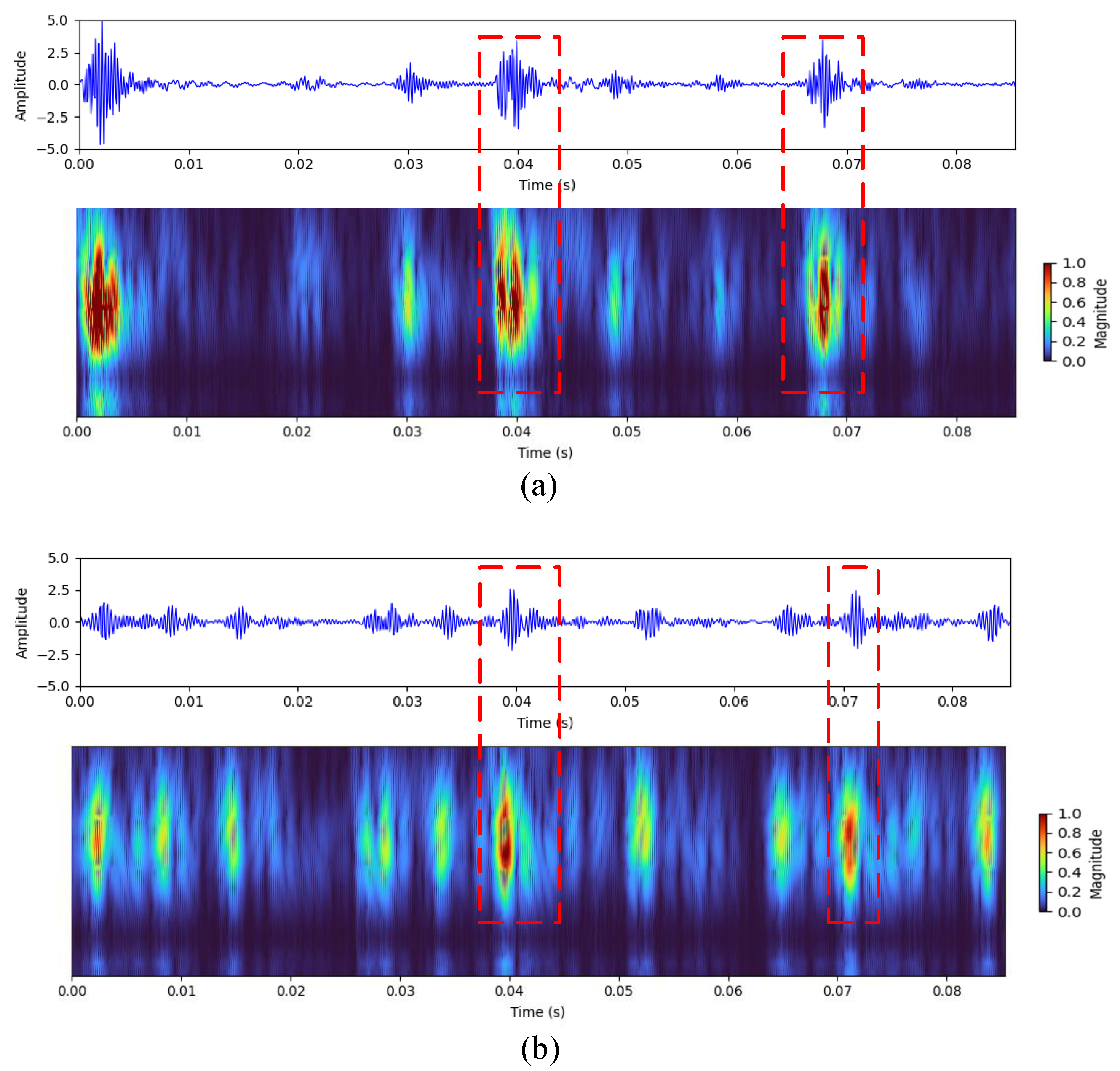
The incorporation of the coordinate attention mechanism was pivotal to the model’s further performance improvement. As shown in Figure 11, which visualizes the attention weights when the model processed outer and inner ring fault signals, the highlighted regions exhibited a high degree of spatiotemporal consistency with the transient impulse peaks caused by fault impacts in the raw signal. Rather than merely propagating features, the mechanism learned and prioritized the importance of each location in the feature map. It enhanced feature channels rich in critical fault information while suppressing irrelevant noise, thereby making the entire model’s information flow more efficient.

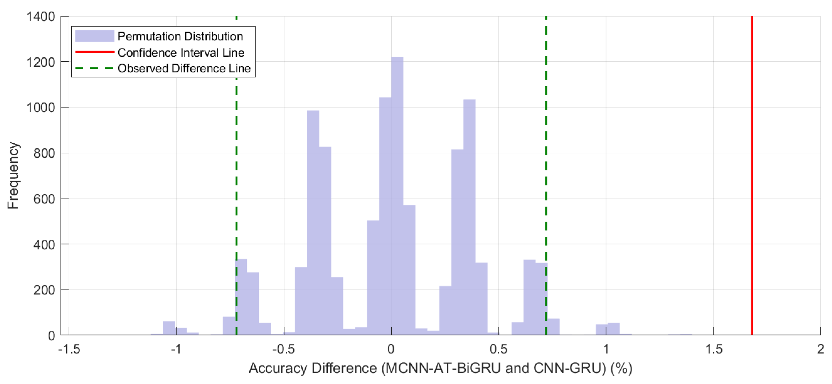
Furthermore, a permutation test was performed on the classification accuracy of the proposed MCNN-AT-BiGRU model relative to the CNN-GRU model. The test was based on 10 independent runs with 10,000 permutation resamplings, and the results are shown in Figure 12. Analysis revealed that the permutation distribution of accuracy under the null hypothesis exhibited an approximately normal shape centered around zero, indicating that if the performance of the two models were equivalent, differences would be expected to cluster near zero. However, the observed accuracy advantage of +1.66% lay far in the right extreme tail of the distribution and fell entirely outside the confidence interval derived from the permutation distribution. This result suggests that the observed difference is highly unlikely to be due to random variance (p < 0.01), leading to a rejection of the null hypothesis. Therefore, the 1.66% performance improvement achieved by the MCNN-AT-BiGRU model is statistically significant, confirming the effectiveness of the proposed model enhancement.

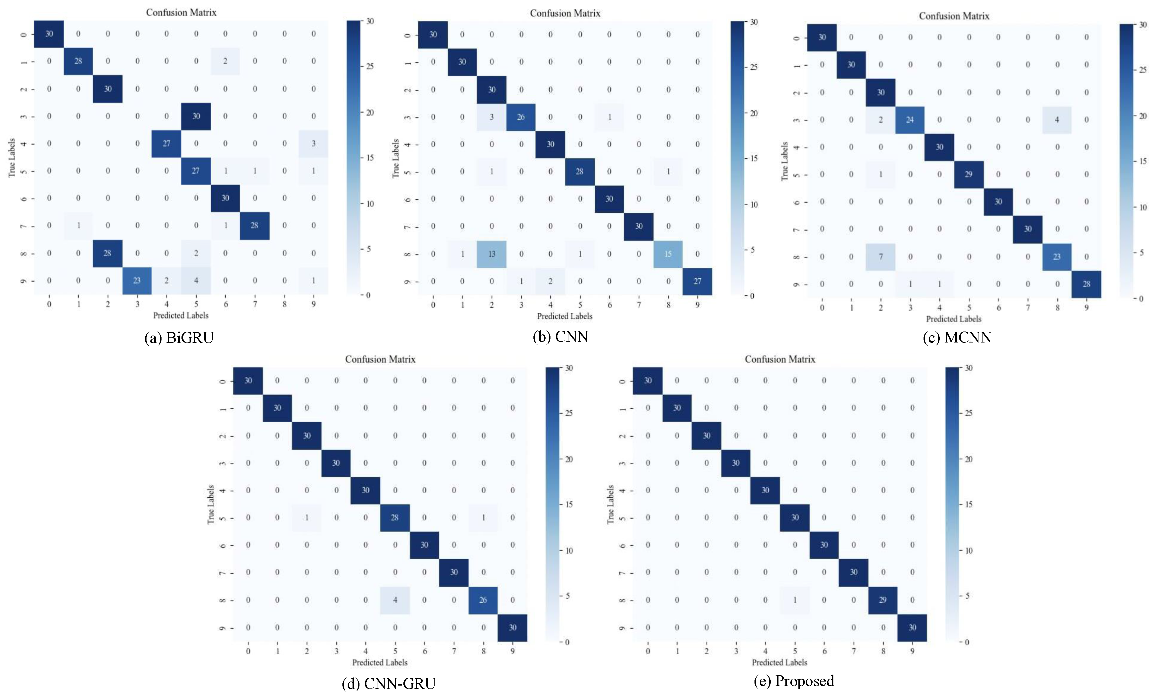
We selected Dataset B to further validate the model. In addition to accuracy, the metrics of precision, recall, and F1-score were also introduced. Similarly, ten repeated experiments were conducted, and the average value was taken as the final result. The specific experimental results are summarized in

Table 7. Performance comparison of different classification models on Dataset B.

Model	Accuracy (%)	Precision (%)	Recall (%)	F1-Score (%)
BiGRU	67.23	63.85	67.23	65.50
CNN	92.34	93.18	92.34	92.76
MCNN	94.45	94.96	94.45	94.70
CNN-GRU	97.36	97.52	97.36	97.44
Proposed	99.72	99.83	99.72	99.77

. Moreover, Figure 13 shows the confusion matrices of different methods, and the proposed model can distinguish the health conditions of these ten types of bearings, which further proves the superiority of the model structure.

The proposed method innovatively integrated multi-scale convolutional structures with attention mechanisms. Multi-scale convolutional layers captured hierarchical spatial features, whereas attention weighting optimized the feature representation. Bidirectional gated recurrent networks further excavated the temporal features. This hierarchical feature learning structure significantly enhanced the feature extraction capability of the model, thereby achieving optimal diagnostic results under stable working conditions, which fully illustrated the validity of the proposed method.

4.3. Noise Interference Scenario Experiment

The vibration signals of rolling bearings collected in industrial fields are often affected by environmental noise. During the initial stages of a fault occurrence, weak fault characteristics are prone to noise. This results in the masking of the critical fault information.

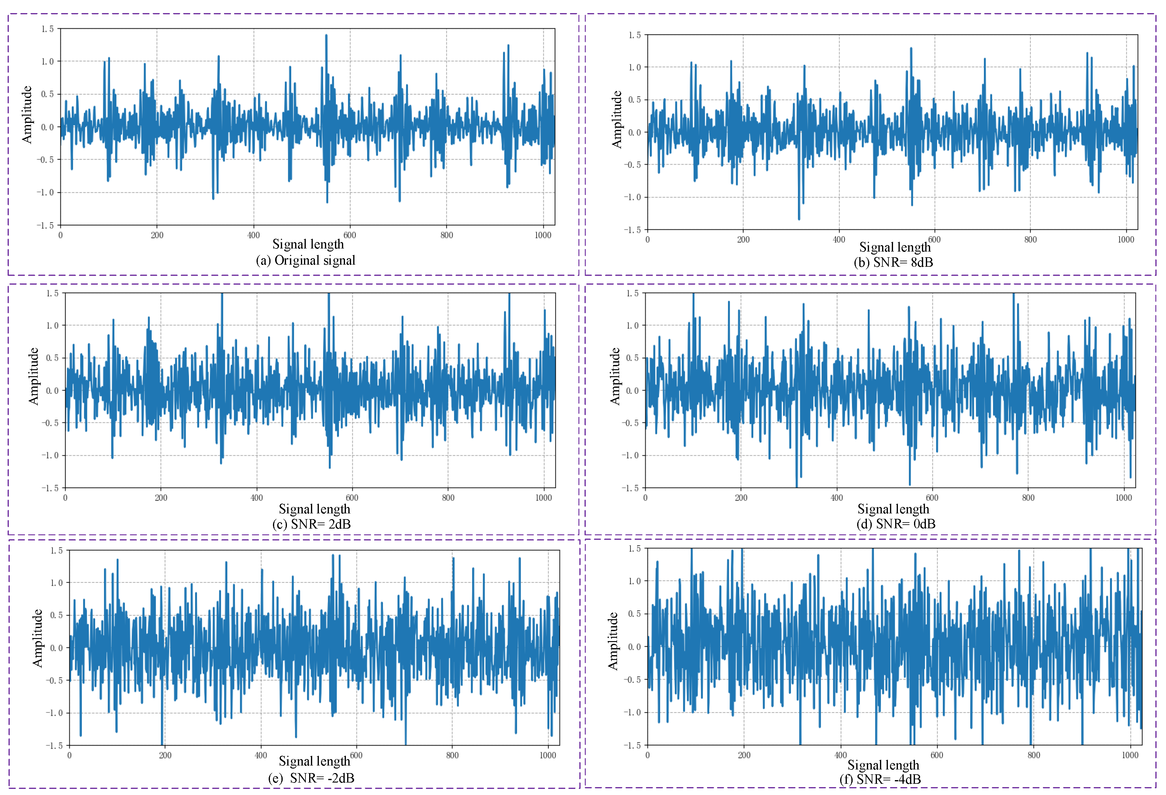
To evaluate the diagnostic performance of models in noisy environments, this study introduced Gaussian white noise to perturb the experimental datasets. Different noise intensities were simulated by adjusting the signal-to-noise ratio (SNR) parameter. Taking an inner race fault sample with a damage diameter of 0.178 mm as an example, Figure 14 illustrates the original signal and noise-contaminated signals at different SNRs. Distinctive fault characteristics were clearly observable in the original signal. However, these characteristics became progressively obscured after the noise injection. As the SNR decreased, the masking effect on the fault features increased significantly. Consequently, the difficulty of fault identification increased correspondingly.

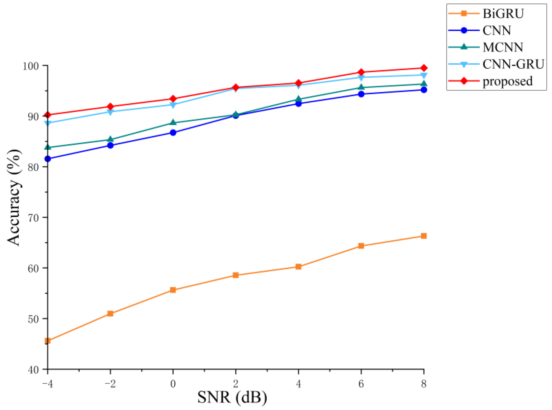
Dataset B was selected for the noise interference experiments. Gaussian white noise with SNRs ranging from −4 dB to 8 dB was injected to simulate varying interference intensities. The experimental parameters were consistent with those of previous configurations to ensure comparability. To ensure result reliability, average values from 10 repeated trials were adopted as final evaluation metrics. Each trial involved 150 iterations for comprehensive assessment. Figure 15 illustrates performance comparison results of different models under varying SNR conditions.

The results showed that the diagnostic accuracy of all the models progressively improved with increasing SNR. Among them, the BiGRU method exhibited suboptimal overall performance. Its accuracy notably lagged behind that of the comparative methods, particularly in low-SNR regions. In contrast, the CNN and MCNN architectures demonstrated stronger noise resistance. This advantage primarily stems from the convolution and pooling operations, which extracted more robust features. These operations suppressed noise interference during signal processing. The CNN-GRU model combined spatial feature extraction from convolutional layers with the temporal modeling capabilities of GRU networks. This hybrid approach achieved superior performance compared with the standalone CNN and MCNN frameworks. The proposed method maintained the leading performance across all the SNR levels. It sustained approximately 90% accuracy even under negative SNR conditions.

Although the aforementioned experiment illustrated the significant robustness of the proposed MCNN-AT-BiGRU model against Gaussian white noise, the acoustic environments in industrial settings are often more complex. As an idealized assumption, Gaussian white noise has a power spectral density that is uniformly distributed across frequencies. In contrast, the background noise in practical mechanical systems typically exhibits specific frequency characteristics. For instance, pink noise and Brownian noise, whose energy is predominantly concentrated in the low-frequency region, more realistically simulate the random interference generated by physical processes such as bearing wear and structural resonance. Furthermore, blue noise, as another typical type of colored noise, possesses an energy distribution opposite to that of pink noise, increasing with frequency. It is often used to simulate high-frequency-dominated interference, such as certain types of electromagnetic interference or high-frequency meshing noise. These types of noise form a continuum of energy distribution from low to high frequencies, providing a more realistic scenario for a comprehensive assessment of the diagnostic model’s robustness.

To evaluate the model’s performance in noise environments that more closely resemble industrial realities, this study incorporated diagnostic experiments under colored noise interference. The SNR was set to 2 dB, with all the other parameters remaining unchanged in the experiment. The average accuracy of ten repeated experiments was taken as the evaluation metric. The results are summarized in

Table 8. Average accuracy of the model across different noise types.

Model	Noise Type
	White Noise	Pink Noise	Brownian Noise	Blue Noise
BiGRU	60.56%	58.73%	53.34%	59.64%
CNN	90.03%	85.93%	83.46%	87.05%
MCNN	91.25%	88.21%	85.15%	89.82%
CNN-GRU	94.45%	90.57%	87.33%	91.42%
Proposed	95.87%	93.95%	92.75%	94.36%

.

As clearly evidenced in Table 8, under the condition of SNR = 2 dB, the proposed MCNN-AT-BiGRU model consistently achieved the highest diagnostic accuracy across all four noise environments. Under the most interfering Brownian noise and pink noise, the proposed model achieved accuracy advantages of 5.42% and 3.38%, respectively, compared with the suboptimal-performing CNN-GRU, which highlighted the critical role of its attention mechanism in capturing transient pulses from strong background noise. Under blue noise, the accuracy of all the models is higher than that under other colored noises, even approaching the level under Gaussian white noise. The proposed model remained leading with an accuracy of 94.36%, which indicated that its multi-scale convolutional structure could effectively extract high-frequency detailed features. The proposed model exhibited stable performance under noises with different energy distributions. Its symmetric network architecture and attention mechanism jointly ensured that it could accurately focus on the essential features of faults, whether in Brownian and pink noises with energy concentrated in low frequencies or in blue noise with energy concentrated in high frequencies. These results supported the effectiveness of the proposed method in terms of robust diagnostic capability under high-noise environments.

4.4. Variable Operating Conditions Scenario Experiment

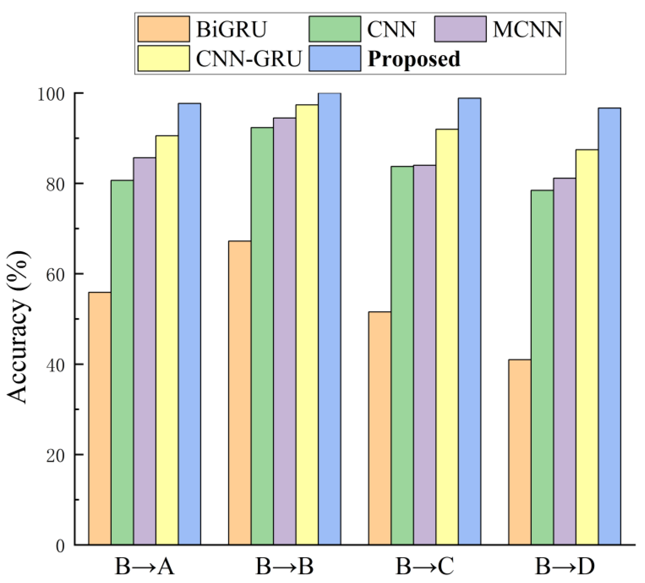
To validate the cross-condition adaptability of the proposed method, datasets A, B, C, and D were used to simulate different load conditions. Specifically, Dataset B under the 1 hp load condition served as the training set for model parameter optimization. Datasets A, C, and D under 0 hp, 2 hp, and 3 hp load conditions were subsequently used to evaluate the model generalization performance. The notation “B→C” denoted training on Dataset B and testing on Dataset C for fault diagnosis. The experimental parameters remained consistent with previous configurations to ensure methodological uniformity. The reliability of the results was ensured through averaged metrics from 10 repeated trials, each involving 150 iterations. Figure 16 presents performance comparisons of the various models under varying operational conditions.

The results illustrated diagnostic accuracy degradation across all the models in cross-condition scenarios (“B→A”, “B→C”, and “B→D”) compared to same-condition testing (“B→B”). This confirmed that operational condition variations significantly increased the diagnostic difficulty. Regarding model performance, BiGRU exhibited the poorest results across all the test scenarios. This reflected its inadequate adaptability to changes in operational conditions. Although outperforming BiGRU, CNN and MCNN still showed noticeable performance degradation under cross-condition settings. The CNN-GRU illustrated relative advantages in specific scenarios (e.g., “B→C” and “B→D”). Nevertheless, its overall performance was inferior to that of the proposed method. The proposed method consistently achieved optimal performance across all the test conditions, demonstrating more significant advantages when there were large differences in working conditions. This validated exceptional cross-condition adaptability and generalization capabilities.

4.5. Generalization Performance Experiment for Different Bearings

In practical industrial applications, bearing faults exhibit diverse generation mechanisms and characteristics. This necessitates the use of diagnostic models to recognize known fault patterns and accurately classify similar fault types.

An additional bearing fault dataset from Jiangnan University was incorporated to evaluate the cross-type fault diagnosis capability of the proposed model [3]. The test bearings were N205EM cylindrical roller bearings, with simulated faults introduced via wire-electrical discharge machining to create 0.3 mm × 0.05 mm (width × depth) grooves on the outer ring, inner ring, and roller surfaces. A cross-validation scheme was implemented through bidirectional testing between the different bearing-type datasets. Initially, the CWRU bearing dataset (Dataset P) was designated as the source domain, whereas the Jiangnan University bearing dataset (Dataset Q) served as the target domain for transfer fault diagnosis. Conversely, Dataset Q was configured as the source domain, with Dataset P acting as the target domain.

Owing to the structural differences between the Jiangnan University and CWRU datasets, the CWRU data were recalibrated to align with the experimental requirements. Specifically, faults with a defect diameter of 0.356 mm on the outer ring, inner ring, and roller at a rotational speed of 1750 r/min were selected. The number of classification categories in the DL model architecture was adjusted from 10 to 4 to accommodate the dataset consistency. The specifications of the key dataset are listed in

Table 9. Transfer dataset.

Dataset	Bearing Type	Fault Type	Rotational Speed
Dataset P	SKF6205 deep groove ball bearing	Normal	1750 r/min
		Roller fault
		Outer ring fault
		Inner ring fault
Dataset Q	N205EM cylindrical roller bearing	Normal	1000 r/min
		Roller fault
		Outer ring fault
		Inner ring fault

.

During the data preprocessing stage, distinct sampling strategies were implemented for both datasets. Dataset P from the CWRU continued to use overlapping sampling techniques. This approach simulated industrial scenarios with limited fault samples. For Jiangnan University Dataset Q, sequential sampling was applied directly to the drive-end vibration signals. Ultimately, 200 samples per fault category were obtained from each dataset, and each sample comprised 1024 consecutive sampling points. Preprocessed samples from Datasets P and Q were used separately for model training. The complete training workflow is illustrated in Figure 17.

Dataset P from CWRU and Dataset Q from Jiangnan University were, respectively, used as source-domain training data to construct a basic model and save the parameters of the feature extraction layer. During model transfer phase, all the parameters except batch normalization and fully connected layers remained frozen. Only 20% of the target-domain samples were utilized for fine-tuning trainable layer parameters. The remaining 80% of the target-domain data was reserved for performance evaluation. The diagnostic accuracies of the four models under different source–target domain configurations are summarized in

Table 10. Model architecture parameters.

Model	BiGRU	CNN	MCNN	CNN-GRU	Proposed
P→Q	52.46%	76.36%	80.23%	85.23%	92.52%
Q→P	56.23%	83.89%	87.34%	90.62%	98.76%

.

The results in Table 10 show the superior performance of the proposed method in cross-type transfer experiments. Diagnostic accuracy rates of 92.52% and 98.76% were achieved, significantly outperforming those of the comparative models. This established enhanced cross-domain generalization capabilities of the proposed method. Further analysis revealed higher diagnostic accuracy when Dataset Q served as the source domain and Dataset P as the target domain. This superiority stemmed from fundamental differences in data structures and sampling strategies between Dataset P and Dataset Q. Dataset Q possesses a greater sample abundance and a relatively sparse sample space distribution. These characteristics enabled the models to learn more generalized feature representations during the source-domain training. Under conditions of favorable source-domain sample sparsity, only a small number of the target-domain fault samples were sufficient for fine-tuning. The accurate identification of similar faults across different bearing types and damage sizes was achieved. This result illustrated the transfer capabilities of the method in cross-domain bearing fault diagnosis.

5. Conclusions

This study proposes an intelligent fault diagnosis framework based on virtual–physical data collaborative optimization. Initially, leveraging the geometric symmetry of rolling bearings, digital twin technology is used to establish a DT model of rolling bearings to simulate various fault modes and their evolution processes, and to generate simulation data to balance the distribution of fault samples in practical applications. Subsequently, a symmetrically parallel MCNN-AT-BiGRU network architecture is constructed. This architecture combines the spatial and temporal feature extraction capabilities through an integrated design. An attention mechanism is incorporated after the MCNN module to enhance the fault impulse characteristics. This mechanism converts critical fault information into attention weights for feature modulation. These optimized weights act on the original feature matrices to facilitate advanced feature learning by the BiGRU.

The experimental results indicate that the method proposed here shows better diagnostic capabilities under diverse fault conditions. The model also exhibits strong transfer learning capability and generalization performance. This provides an effective solution for bearing fault diagnosis, thereby ensuring the safe and efficient operation of bearings.

It is also important to acknowledge several limitations of the current study. These limitations clarify the scope of our present findings and point to a clear direction for future research. First, the DT model uses a simplified rectangular geometry to represent bearing spalls. This simplification fails to fully capture the intricate morphologies of real-world single damage. Moreover, it struggles to reflect the interactive characteristics and complex coexistence states of simultaneous faults. Second, the current noise-resistance experiments mainly focus on additive white Gaussian noise and included some colored noises. They do not address more prevalent and complex industrial interferences. Addressing these limitations will be a core focus of our subsequent research. Thus, future work will not only assess the model’s long-term reliability under extreme conditions but also extend the current framework to diagnose simultaneous faults.

References

1. Ding, L.; Li, Q. Fault diagnosis of rotating machinery using novel self-attention mechanism TCN with soft thresholding method. Meas. Sci. Technol. 2024, 35, 047001. [Google Scholar] [CrossRef]
2. Yu, Y.; Zeng, R.; Xue, Y.; Zhao, X. Optimization strategy of rolling mill hydraulic roll gap control system based on improved particle swarm PID algorithm. Biomimetics 2023, 8, 143. [Google Scholar] [CrossRef] [PubMed]
3. Zhao, Z.; Li, T.; Wu, J.; Sun, C.; Wang, S.; Yan, R.; Chen, X. Deep learning algorithms for rotating machinery intelligent diagnosis: An open source benchmark study. ISA Trans. 2020, 107, 224–255. [Google Scholar] [CrossRef]
4. Brahmbhatt, P.; Patel, R.; Maheshwari, A.; Gudi, R.D. Improved fault detection and diagnosis using graph auto encoder and attention-based graph convolution networks. Digit. Chem. Eng. 2024, 11, 100158. [Google Scholar] [CrossRef]
5. Gajjar, A.; El-Farra, N.H. Machine Learning-Based Estimation and Accommodation of Multiple Sensor Faults in Sampled-Data Process Systems. In Proceedings of the 2024 American Control Conference (ACC), Toronto, ON, Canada, 10–12 July 2024; pp. 3043–3048. [Google Scholar] [CrossRef]
6. Shahnazari, H. Fault diagnosis of nonlinear systems using recurrent neural networks. Chem. Eng. Res. Des. 2020, 153, 233–245. [Google Scholar] [CrossRef]
7. Xie, X.; Merino, J.; Moretti, N.; Pauwels, P.; Chang, J.Y.; Parlikad, A. Digital twin enabled fault detection and diagnosis process for building HVAC systems. Autom. Constr. 2023, 146, 104695. [Google Scholar] [CrossRef]
8. Zhang, J.; Wang, Y.; Yang, Y.; Ma, Y.; Dai, Z. Fault diagnosis and intelligent maintenance of industry 4.0 power system based on internet of things technology and thermal energy optimization. Therm. Sci. Eng. Prog. 2024, 55, 102902. [Google Scholar] [CrossRef]
9. Shandhoosh, V.; Chakrapani, G.; Sugumaran, V.; Ramteke, S.M.; Marian, M. Intelligent fault diagnosis for tribo-mechanical systems by machine learning: Multi-feature extraction and ensemble voting methods. Knowl. Based Syst. 2024, 305, 112694. [Google Scholar] [CrossRef]
10. Wang, H.; Zheng, J.; Xiang, J. Online bearing fault diagnosis using numerical simulation models and machine learning classifications. Reliab. Eng. Syst. Saf. 2023, 234, 109142. [Google Scholar] [CrossRef]
11. Wang, J.; Gao, D.; Zhu, S.; Wang, S.; Liu, H. Fault diagnosis method of photovoltaic array based on support vector machine. Energy Sources Part A Recover. Util. Environ. Eff. 2023, 45, 5380–5395. [Google Scholar] [CrossRef]
12. Wang, S.; Zhou, Y.; Ma, Z. Research on fault identification of high-voltage circuit breakers with characteristics of voiceprint information. Sci. Rep. 2024, 14, 9340. [Google Scholar] [CrossRef]
13. Chen, F.; Cheng, M.; Tang, B.; Chen, B.; Xiao, W. Pattern recognition of a sensitive feature set based on the orthogonal neighborhood preserving embedding and adaboost_SVM algorithm for rolling bearing early fault diagnosis. Meas. Sci. Technol. 2020, 31, 105007. [Google Scholar] [CrossRef]
14. Kou, L.; Liu, C.; Cai, G.; Zhou, J.; Yuan, Q. Data-driven design of fault diagnosis for three-phase PWM rectifier using random forests technique with transient synthetic features. IET Power Electron. 2020, 13, 3571–3579. [Google Scholar] [CrossRef]
15. Liu, J.; Cai, B.; Yan, S.; Sun, P. Transformer fault diagnosis based on the improved QPSO and random forest. Meas. Sci. Technol. 2024, 35, 096206. [Google Scholar] [CrossRef]
16. Yu, Z.; Zhang, B.; Hu, G.; Chen, Z. Early fault diagnosis model design of reciprocating compressor valve based on multiclass support vector machine and decision tree. Sci. Program. 2022, 2022, 7486271. [Google Scholar] [CrossRef]
17. Nguyen, T.D.; Nguyen, T.H.; Do, D.T.B.; Pham, T.H.; Liang, J.W.; Nguyen, P.D. Efficient and explainable bearing condition monitoring with decision tree-based feature learning. Machines 2025, 13, 467. [Google Scholar] [CrossRef]
18. Cui, L.; Sun, M.; Zha, C. Early bearing fault diagnosis based on the improved singular value decomposition method. Int. J. Adv. Manuf. Technol. 2023, 124, 3899–3910. [Google Scholar] [CrossRef]
19. Zhang, Y.; Liu, W.; Gu, H.; Alexisa, A.; Jiang, X. A novel wind turbine fault diagnosis based on deep transfer learning of improved residual network and multi-target data. Meas. Sci. Technol. 2022, 33, 095007. [Google Scholar] [CrossRef]
20. Zhu, R.; Wang, M.; Xu, S.; Li, K.; Han, Q.; Tong, X.; He, K. Fault diagnosis of rolling bearing based on singular spectrum analysis and wide convolution kernel neural network. J. Low Freq. Noise Vib. Act. Control 2022, 41, 1307–1321. [Google Scholar] [CrossRef]
21. Chen, X.; Zhang, B.; Gao, D. Bearing fault diagnosis base on multi-scale CNN and LSTM model. J. Intell. Manuf. 2021, 32, 971–987. [Google Scholar] [CrossRef]
22. Intelligent fault diagnosis of machines with small & imbalanced data: A state-of-the-art review and possible extensions. ISA Trans. 2022, 119, 152–171. [CrossRef]
23. Zhang, X.; He, C.; Lu, Y.; Chen, B.; Zhu, L.; Zhang, L. Fault diagnosis for small samples based on attention mechanism. Measurement 2022, 187, 110242. [Google Scholar] [CrossRef]
24. Peng, F.; Zheng, L.; Peng, Y.; Fang, C.; Meng, X. Digital Twin for rolling bearings: A review of current simulation and PHM techniques. Measurement 2022, 201, 111728. [Google Scholar] [CrossRef]
25. Xia, M.; Shao, H.; Williams, D.; Lu, S.; Shu, L.; de Silva, C.W. Intelligent fault diagnosis of machinery using digital twin-assisted deep transfer learning. Reliab. Eng. Syst. Saf. 2021, 215, 107938. [Google Scholar] [CrossRef]
26. Yan, S.; Zhong, X.; Shao, H.; Ming, Y.; Liu, C.; Liu, B. Digital twin-assisted imbalanced fault diagnosis framework using subdomain adaptive mechanism and margin-aware regularization. Reliab. Eng. Syst. Saf. 2023, 239, 109522. [Google Scholar] [CrossRef]
27. Zhang, Y.; Ji, J.; Ren, Z.; Ni, Q.; Gu, F.; Feng, K.; Yu, K.; Ge, J.; Lei, Z.; Liu, Z. Digital twin-driven partial domain adaptation network for intelligent fault diagnosis of rolling bearing. Reliab. Eng. Syst. Saf. 2023, 234, 109186. [Google Scholar] [CrossRef]
28. Li, S.; Jiang, Q.; Xu, Y.; Feng, K.; Wang, Y.; Sun, B.; Yan, X.; Sheng, X.; Zhang, K.; Ni, Q. Digital twin-driven focal modulation-based convolutional network for intelligent fault diagnosis. Reliab. Eng. Syst. Saf. 2023, 240, 109590. [Google Scholar] [CrossRef]
29. Ming, Z.; Tang, B.; Deng, L.; Yang, Q.; Li, Q. Digital twin-assisted fault diagnosis framework for rolling bearings under imbalanced data. Appl. Soft Comput. 2025, 168, 112528. [Google Scholar] [CrossRef]
30. Zhu, H.M.; Chen, W.F.; Zhu, R.P.; Zhang, L.; Gao, J.; Liao, M.J. Dynamic analysis of a flexible rotor supported by ball bearings with damping rings based on FEM and lumped mass theory. J. Cent. South Univ. 2020, 27, 3684–3701. [Google Scholar] [CrossRef]
31. Zhao, D.; Tian, C.; Fu, Z.; Zhong, Y.; Hou, J.; He, W. Multi scale convolutional neural network combining BiLSTM and attention mechanism for bearing fault diagnosis under multiple working conditions. Sci. Rep. 2025, 15, 13035. [Google Scholar] [CrossRef]
32. Hou, Q.; Zhou, D.; Feng, J. Coordinate Attention for Efficient Mobile Network Design. In Proceedings of the IEEE/CVF Conference on Computer Vision and Pattern Recognition, Nashville, TN, USA, 20–25 June 2021; pp. 13713–13722. [Google Scholar] [CrossRef]
33. Smith, W.A.; Randall, R.B. Rolling element bearing diagnostics using the Case Western Reserve University data: A benchmark study. Mech. Syst. Signal Process. 2015, 64, 100–131. [Google Scholar] [CrossRef]
34. Ding, C.; Wang, F.; Li, S.; Jiang, C.; Ma, P. Three-Core Cable Fault Line Identification Based on Ground Wire Current and BiGRU-ResNet-MA. IEEE Access 2024, 12, 136120–136130. [Google Scholar] [CrossRef]
35. Sun, Y.; Zhang, J.; Yu, Z.; Zhang, Y.; Liu, Z. Bidirectional long short-term neural network based on the attention mechanism of the residual neural network (ResNet–BiLSTM–attention) predicts porosity through well logging parameters. ACS Omega 2023, 8, 24083–24092. [Google Scholar] [CrossRef] [PubMed]
Figure 1. Nonlinear dynamics model of rolling bearings.
Symmetry 17 01803 g001
Figure 2. Diagram of local defect.
Symmetry 17 01803 g002
Figure 3. Time-domain diagrams and corresponding envelope spectra of simulated signals and measured signals under the outer ring fault.
Symmetry 17 01803 g003
Figure 4. Time-domain diagrams and corresponding envelope spectra of simulated signals and measured signals under the inner ring fault.
Symmetry 17 01803 g004
Figure 5. Time-domain diagrams and corresponding envelope spectra of simulated signals and measured signals under the roller fault.
Symmetry 17 01803 g005
Figure 6. Overall framework diagram of fault diagnosis.
Symmetry 17 01803 g006
Figure 7. MCNN-AT-BiGRU model architecture diagram.
Symmetry 17 01803 g007
Figure 8. Signal attention mechanism architecture diagram.
Symmetry 17 01803 g008
Figure 9. Signal acquisition flowchart.
Symmetry 17 01803 g009
Figure 10. Bearing fault diagnosis model test rig and faulty bearing types. Abbreviation: NOR, normal; ROF, roller fault; IRF, inner ring fault; ORF, outer ring fault.
Symmetry 17 01803 g010
Figure 11. Coordinate attention weight visualization: (a) the outer ring fault, (b) the inner ring fault, where the red dashed lines represent the comparative visualization of attention weights for vibration signals.
Symmetry 17 01803 g011
Figure 12. Permutation test distribution of accuracy differences.
Symmetry 17 01803 g012
Figure 13. Confusion matrix of different models in Dataset B.
Symmetry 17 01803 g013
Figure 14. Original signals and signals with added noise at different SNRs.
Symmetry 17 01803 g014
Figure 15. Fault diagnosis results of various models under different SNRs.
Symmetry 17 01803 g015
Figure 16. Fault diagnosis results under varying operational conditions scenario.
Symmetry 17 01803 g016
Figure 17. Schematic diagram of the transfer process.
Symmetry 17 01803 g017