Article

Symmetry-Preserving Optimization of Differentially Private Machine Learning Based on Feature Importance

1
Department of Information Management, Lunghwa University of Science and Technology, Taoyuan 33306, Taiwan
2
Department of Management Information Systems, National Chung Hsing University, Taichung 40227, Taiwan
3
Department of Computer Science and Information Engineering, Asia University, Taichung 41354, Taiwan
4
Department of Medical Research, China Medical University Hospital, China Medical University, Taichung 40402, Taiwan
*
Author to whom correspondence should be addressed.
Symmetry 2025, 17(10), 1747; https://doi.org/10.3390/sym17101747
Submission received: 7 September 2025 / Revised: 13 October 2025 / Accepted: 13 October 2025 / Published: 16 October 2025

Abstract

Symmetry plays a critical role in preserving the structural balance and statistical integrity of datasets, particularly in privacy-preserving machine learning. Differential privacy introduces random noise to individual data points to ensure privacy while maintaining the overall symmetry of statistical distributions. However, excessive noise can reduce the utility of data, model accuracy, and computational efficiency. This study proposes a symmetry-preserving optimization framework for differentially private machine learning by integrating feature importance and t-SNE (t-distributed Stochastic Neighbor Embedding), UMAP (Uniform Manifold Approximation and Projection), and PCA (Principal Component Analysis), respectively. Feature importance derived from a random forest selects high-value features to improve data relevance. At the same time, t-SNE preserves geometric symmetry by retaining local and global structures more effectively than PCA or UMAP. Therefore, t-SNE is the best feature extraction method for dimensionality reduction in the proposed scheme. Experimental results demonstrate that the t-SNE method significantly enhances model performance under differential privacy, showing improved accuracy and reduced computational time compared to PCA and UMAP while preserving the underlying symmetry of the data distributions.

1. Introduction

In recent years, data has become a crucial asset in industrial competition. Websites, mobile applications, and even shopping mall membership systems are extensively collecting user data from various sources. Through comprehensive data analysis, companies can gain insights into consumer behavior and preferences, enabling them to tailor product advertisements and services to meet individual needs.
Traditionally, machine learning requires that training data be centralized on a specific server or machine. However, the rapid development of mobile technologies and the widespread use of smart devices have led to a dramatic increase in both the volume and distribution of data. At the same time, growing global awareness of data privacy has made data collection and usage increasingly difficult [1].
For instance, the European Union introduced the General Data Protection Regulation (GDPR) in 2018 [2], widely regarded as the most stringent data protection law in history. The GDPR outlines strict rules regarding the handling of personal data, including requirements for pseudonymization or anonymization, default privacy settings, transparency in data collection and usage, and the right of individuals to withdraw consent or request data deletion at any time [3]. Furthermore, companies must notify authorities of data breaches within 72 h. These regulations have significantly impacted the marketing and data strategies of industries across Europe, including technology, finance, and retail.
For data-driven enterprises such as Google, these developments posed a significant challenge. In response, Google proposed Federated Learning in 2016 [4,5,6,7,8], a novel decentralized machine learning framework. Federated learning enables multiple devices or institutions to collaboratively train a shared model without exchanging raw data collaboratively, thereby preserving user privacy [9,10]. Depending on the application scenario, federated learning can be categorized into consumer-oriented (To-C) and enterprise-level (To-B) solutions. For example, Google applies federated learning to improve the accuracy of predictive text input by learning usage patterns directly from users’ mobile devices [8].
From a theoretical perspective, federated learning introduces a form of symmetry in data collaboration. Despite the distributed nature of the participants, all parties contribute equally to the training of a shared global model without exposing their private data. This symmetrical structure in data processing not only enhances fairness and privacy but also opens new research avenues in algorithm optimization and distributed systems. In the context of federated learning, symmetry manifests in the balanced contribution of data owners and the uniform treatment of local models during aggregation, which are crucial for maintaining the integrity and robustness of the system.
In summary, the advancement of increasing computational capabilities has made machine learning indispensable in various domains. Nevertheless, the introduction of regulations such as the GDPR has shifted attention toward the dual goals of data utility and privacy preservation. Federated learning offers a promising solution to this challenge, and its inherent symmetrical framework highlights the balance between distributed computation and centralized performance. This idea continues to attract attention across both academic and industrial communities.
The rest of this paper is organized as follows: Section 2 reviews related works on differential privacy. To improve the performance of differential privacy in machine learning, we propose a scheme that utilizes various data preprocessing methods to reduce the dataset’s size and dimension in Section 3. In Section 4, we experiment to compare the computational time and accuracy of three dimensionality reduction methods—PCA (Principal Component Analysis), t-SNE (t-distributed Stochastic Neighbor Embedding), and UMAP (Uniform Manifold Approximation and Projection). Finally, Section 5 concludes this paper.

2. Related Works

With the development of science and technology and the rise of privacy awareness, various data analysis methods using machine learning have become increasingly popular, including data mining, data prediction, and data clustering. Although these methods can quickly calculate the meaning of a large amount of data, privacy leakage may occur during the training process [11].
Cuzzocrea et al. identified the threats and development status of data mining [1]. Google proposed the concept of federated learning in 2016 [4,5,6,7,8]. They designed a federated training algorithm called Federated Averaging. First, in each round of training, the central server sends a determined global model to the participating users in that round. After the participating users receive this model, they train it based on their local data (for example, the typing records of users on each device using the input method), calculate the gradient using SGD (Stochastic Gradient Descent), and update the model parameters. After the model converges, it is sent back to the central server. After receiving the updated model from the participating users, the central server averages these parameters to generate a new model. Finally, the central server sends the updated model back to each user, and each user updates their model accordingly. Lin et al. introduced various attacks and defense methods in detail [12].
In this process, privacy leakage is prone to occur. Chen et al. studied the privacy problem of federated learning from the perspective of models [13]. Mothukuri et al. detailed the operation mode of federated learning [4] and the concept of federated learning classification (vertical, horizontal, and transfer federated learning). They mentioned the security issues, privacy concerns, and various attack methods associated with federated learning. They explained in detail the threats of various attack methods and how to defend against them. They proposed various privacy issues that federated learning will face in the future and compared them with those of decentralized machine learning. Li et al. [6] and Li et al. [7] proposed the potential and possible crises of federated learning and introduced its applications.
Differential privacy can effectively address the above privacy issues. Li et al. outlined the mechanism, algorithm, and noise addition method of differential privacy, as well as its application in machine learning, including data mining and classification [14]. Ji et al. sorted out the interaction between differential privacy and machine learning, including how machine learning algorithms protect privacy and data release mechanisms [15]. Some theoretical algorithms are also introduced, such as the upper limit of the loss function of the differential privacy algorithm and the content that the differential privacy algorithm can learn. Finally, several open questions are raised, including how to merge public data, how to handle missing data in private datasets, and whether the utility of differentially private machine learning algorithms can reach a comparable level to that of the corresponding non-differentially private algorithms as the number of samples increases.
In 2023, Dong et al. proposed a holistic scheme to set a more optimal error and privacy budget allocation strategy for multiple queries [16]. Their scheme outperforms the composition method in the case of skewed data and a large number of queries. In 2024, Laouir and Imine proposed a distribution-aware online sampling technique to accelerate query execution [17]. Their scheme enables fast response to range queries in the context of horizontal data partitioning (multiple owners) while maintaining end-to-end privacy guarantees and low error.
Its application methods can be roughly divided into two categories. First, noise is added during the machine learning calculation process to prevent parameter leakage, which can cause privacy issues. Abadi et al. proposed a new algorithmic technique for learning and fine-tuning the privacy budget method in the deep learning model of the differential privacy framework [18]. Regarding the gradient parameters generated during training, Xia et al. proposed a gradient-based differential privacy optimizer for deep learning models based on a collaborative training model. To protect privacy, this method requires sanitizing the gradients before using them to update parameters. Ni et al. proposed a differential privacy multi-core DBSCAN clustering method (DP-MCDBSCAN) based on differential privacy and the DBSCAN algorithm [19]. The method requires only two simplified parameters, ϵ -neighborhood (Eps-Neighborhood) and MinPts. Wang et al. applied differential privacy to the matrix decomposition method for solving recommendation problems [20]. For the centralized recommendation scenario, a collaborative filtering model based on matrix decomposition is established, and a matrix decomposition mechanism that satisfies ϵ -differential privacy is proposed. Sharma et al. found that privacy leakage at the edge layer and unauthorized access to private data are common issues affecting privacy. To address this problem, Sharma et al. proposed DP-FCNN, a fuzzy convolutional neural network (FCNN) that incorporates a Laplace mechanism [21]. When the dataset is uploaded by the data owner to the data provider, the data provider will be responsible for adding noise and then encrypting it using Piccolo encryption before uploading it to the cloud.
Second, noise is added to the original dataset. Since differential privacy conforms to the normal distribution, its data still retains the characteristics of being statistically significant after adding noise, making it a robust encryption method. Ji and Elkan proposed a differential privacy mechanism based on importance weighting [22]. This method is primarily designed to mitigate the privacy leakage risk associated with public datasets, particularly medical datasets. If hospitals can make their medical datasets public, it can help more patients and research institutions. Therefore, hospitals will utilize differential privacy and anonymization to encrypt or anonymize datasets and then make them publicly available. However, attackers can obtain the original content of the datasets through various cross-comparison methods. Therefore, Ji and Elkan’s method uses importance weighting to calculate the weight of the data correlation between a non-confidential public dataset and a confidential private dataset. The weight will be regularized, and noise will be added through differential privacy. The weight allows statistical queries to be answered approximately while maintaining data privacy. Through experiments, it has been demonstrated that the method can perform well even when the privacy budget is small and the public and private datasets originate from the same participants.
Recently, Akmese et al. have demonstrated diverse research results in the fields of medical imaging, clinical diagnosis, and information security. Akmese proposed a new random number generator and applied it to sound encryption based on fractional-order chaotic systems, thereby enhancing information security [23]. Akmese developed a privacy-preserving machine learning method for pancreatic cancer diagnosis, striking a balance between data privacy and diagnostic efficacy [24]. Alaca and Akmeşe converted pancreatic tumor CT images into a graph structure and combined it with the whale algorithm and transfer learning classifier to improve tumor detection accuracy [25]. Tozlu et al. proposed a non-invasive method for diagnosing psoriasis based on exhaled breath analysis, demonstrating its potential clinical application [26]. Overall, these studies have not only advanced smart medical diagnostic technology but also expanded the application scope of data privacy and security.

3. The Proposed Scheme

To ensure the privacy and availability of data, this study incorporates Laplace noise into the dataset using the mechanism of differential privacy, thereby preventing privacy leakage while allowing the data to be utilized in machine learning tasks. The Laplace mechanism is widely adopted in differential privacy because it adds noise drawn from the Laplace distribution, which has a mean of zero and a scale proportional to the sensitivity of the query divided by the privacy budget ϵ . This distribution is symmetric and centered, ensuring unbiased perturbation of the data. Its main advantages include (1) theoretical simplicity and strong ϵ -differential privacy guarantee, (2) efficient implementation with low computational overhead, and (3) effective control of noise magnitude via ϵ . However, the disadvantages are that Laplace noise may introduce heavier perturbations compared to Gaussian noise in high-dimensional settings, and excessive noise can degrade model accuracy if ϵ is too small. In this study, we choose the Laplace mechanism because it provides a clear and rigorous privacy guarantee under the pure ϵ -DP framework, which is more suitable for our dataset scale and application scenario [18]. The effects of noise addition are evaluated with respect to several key parameters: the privacy loss parameter ( ϵ ), model accuracy (F1-score and MSE), and computational time under varying noise levels. Since big data analysis requires a balance between immediacy and accuracy, this study further employs data preprocessing methods, including data screening and feature extraction, to mitigate the negative impact of noise on model performance. These steps reduce the size and dimensionality of the dataset, thereby improving both the efficiency and robustness of differential privacy-based machine learning. The overall process architecture is presented in Figure 1.
  • Step 1. Feature Selection:
    • This step involves calculating feature correlation and removing collinear features. We use the correlation analysis to calculate the correlation between features, and we set a threshold to filter out features with too high a correlation, thereby reducing the impact of data correlation and noise.
    • To reduce the correlation and potential noise between features in the data, we utilize information entropy and mutual information as the basis for correlation analysis.
    • By calculating the mutual information value between each pair of features, we can effectively capture linear and nonlinear correlations. First, the continuous variables are appropriately discretized to calculate the mutual information accurately. Then, we calculate the mutual information between all features and construct a matrix of feature mutual information. According to the set mutual information threshold, the features above the threshold are regarded as highly redundant. The lowly redundant are selectively retained, and the other highly redundant are removed to achieve the purpose of feature filtering and data simplification.
    • In this way, we not only effectively reduce collinearity and redundancy in the data but also control unnecessary information overlap between features, thereby reducing the noise level introduced in the model learning process and improving the model’s stability and generalization ability.
  • Step 2. Calculate feature importance based on random forest:
    • To remove unimportant features, we calculate feature importance using the random forest. The features are sorted according to feature importance, and features are removed in order of importance from low to high until the best accuracy is achieved.
    • Assuming there are n features, the feature importance based on random forest will calculate the Gini Impurity of each feature. The so-called Gini Impurity is the probability of misclassifying randomly selected elements in the dataset after randomly labeling them according to the class distribution in the dataset. Its calculation formula is as follows:
      G = i = 1 c P ( i ) × [ ( 1 P ( i ) ]
      where c denotes the total number of classes; P ( i ) denotes the probability of the ith class. Removing or reducing noise with low contribution and less relevant information can effectively reduce the noise scale, improve accuracy, and enhance availability. Moreover, when the noise scale or data volume is reduced, the calculation cost will also decrease, and the mean square error (MSE) of the data query will be lower.
  • Step 3. Reduce the dimension:
    • In reality, most data does not exist in one-dimensional space, but it may exist in a higher-dimensional space. High-dimensional data can lead to the curse of dimensionality. Figure 2 illustrates that as the dimensionality increases, the sample data becomes sparser.
    Figure 2. The higher the dimensionality, the sparser the sample data becomes.
    Figure 2. The higher the dimensionality, the sparser the sample data becomes.
    Symmetry 17 01747 g002
    • We use the following different feature extraction methods for dimensionality reduction:
      1.
      PCA: A standard method for feature extraction is principal component analysis (PCA) [27]. Li et al. optimized PCA using importance assessment. The optimized PCA can perform feature screening and dimensionality reduction, thereby reducing the amount of data required for calculation and significantly reducing calculation time while maintaining or even improving accuracy. PCA linearly transforms the observed values of a series of possibly related variables through orthogonal transformation and projects them into a series of linearly unrelated variable values, which are called principal components. This method can reduce high-dimensional data to low-dimensional data. Its advantages include avoiding the curse of dimensionality, reducing data correlation, reducing calculation time, and improving model accuracy. However, if PCA is not applied to linear data, a large amount of structural information may be lost in the process of projecting the data vector.
      2.
      t-SNE: t-SNE (t-distributed Stochastic Neighbor Embedding) [28] is a nonlinear dimensionality reduction algorithm that uses a t-distribution to define a probability distribution in a low-dimensional space. It is often used for visualization and processing of high-dimensional datasets, and it can effectively alleviate the problem of structural information loss caused by the curse of dimensionality. The t-SNE algorithm consists of three parts.
      (a)
      t-SNE is used to find the similarity between two points in high-dimensional space. This method assigns a higher probability to similar data points while assigning a lower probability to data points with larger differences. Its formula is as follows:
      P j | i = exp ( | | x i x j | | 2 / 2 σ i 2 ) k i exp ( | | x i x k | | 2 / 2 σ i 2 )
      where P j | i is the conditional probability, and x i and x j are the two data points whose similarity is to be calculated. If x i and x j are close to each other, then P j | i is large.
      (b)
      t-SNE defines the similar probability distribution of points in a low-dimensional space. Low-dimensional data often follows a t-distribution (because the t-distribution is robust to outliers) rather than a normal distribution. The formula for t-SNE in low-dimensional space is as follows:
      q j | i = exp ( 1 + | | y i y j | | 2 ) 1 k i exp ( 1 + | | y k y l | | 2 ) 1
      (c)
      After obtaining the probabilities of high-dimensional space and low-dimensional space, the proximity between P j | i and q j | i is calculated. The calculation formula is as follows:
      C = i K L ( p i | | q i ) = i j p j | i log p j | i q j | i
      where p i and q i are the conditional probabilities of high-dimensional space and low-dimensional space, respectively, C is the cost function, KL is the Kullback–Leibler divergence, and the Kullback–Leibler divergence is an indicator to measure the difference in probability distribution.
      Since standard t-SNE is non-parametric and does not provide a natural mapping for unseen/test data, in this study, we adopted the common practice of fitting t-SNE on the training set, then applying the learned embedding to the test set using a parametric approximation approach. This ensures that performance evaluation on the test set is unbiased and feasible within the experimental design.
      3.
      UMAP: Uniform Manifold Approximation and Projection (UMAP) [29] is a dimensionality reduction technique based on the theoretical framework of Riemannian geometry and algebraic topology. Assuming that the available data samples are uniformly distributed in the topological space (or manifold), these limited data samples can be approximated and mapped to a lower-dimensional space. Its visualization and dimensionality reduction capabilities are comparable to t-SNE. Still, its dimensionality reduction time is shorter than t-SNE, and there is no computational limit on the embedding dimension. The UMAP algorithm is based on three assumptions about the dataset: (1) the data is uniformly distributed on the Riemannian manifold; (2) the Riemannian metric is locally constant; and (3) the manifold is interconnected within the region.
      UMAP can be divided into three main steps:
      (a)
      Learning the manifold structure in the high-dimensional space
      Before mapping high-dimensional data to a low-dimensional space, it is necessary to understand what the data looks like in the high-dimensional space. The UMAP algorithm initially employs the nearest neighbor descent method to identify the nearest data point. Here, you can specify the number of neighboring data points to use by adjusting the n_neighbors parameter. UMAP limits the size of local neighborhoods when learning the manifold’s structure to control how UMAP balances the local and global structure of the data. Therefore, it is crucial to adjust the number of n_neighbors.
      UMAP needs to build a graph by connecting the nearest neighbor data points that have been previously determined. The data points are assumed to be uniformly distributed on the manifold, which means that the space between these data points will stretch or shrink depending on the location of the data (whether it is sparse or dense). This means that the distance measure is not universal across the entire space but varies from one region to another.
      (b)
      Find a low-dimensional representation of the manifold structure
      After learning an approximate manifold from a high-dimensional space, the next step of UMAP is to project (map) it to a low-dimensional space. Unlike the first step, this step does not aim to change the distance in the low-dimensional space representation; instead, it seeks to make the distance on the manifold equivalent to the standard Euclidean distance relative to the global coordinate system.
      However, the conversion from variable distance to standard distance will also affect the distance of the nearest neighbor. Therefore, another hyperparameter called min_dist (default value = 0.1) needs to be passed here to define the minimum distance between embedding points. This step controls the minimum distribution of data points and avoids the situation where many data points overlap with each other in the low-dimensional embedding. After specifying the minimum distance, the algorithm can begin searching for a more optimal low-dimensional manifold representation.
      (c)
      Minimize the cost function (cross entropy)
      The ultimate goal of this step is to find the optimal weight values of the edges in the low-dimensional representation. These optimal weight values are determined by minimizing the cross-entropy function, which can be optimized using stochastic gradient descent. UMAP achieves the goal of finding a better low-dimensional manifold representation by minimizing the following cost function:
      C E = e E W h ( e ) log ( W h ( e ) W l ( e ) ) + ( 1 W h ( e ) ) log ( 1 W h ( e ) 1 W l ( e ) )
      C E stands for cross entropy, W h ( e ) stands for the manifold edge weights learned in high-dimensional space, and W l ( e ) stands for the manifold edge weights in low-dimensional space.
      Moreover, this study will explore and compare the accuracy and computational time of the three different feature extraction methods for dimensionality reduction (t-NSE, PCA, and UMAP) mentioned above as dimensionality reduction methods for the proposed scheme.
  • Step 4. Add Laplace noise:
    • In this step, the differential privacy guarantee is achieved through input perturbation, i.e., Laplace noise is directly added to the features of the dataset before they are used for machine learning tasks. This ensures that the original data cannot be reverse-engineered while still allowing subsequent steps, such as feature selection and dimensionality reduction, to operate on privatized inputs.
      For a dataset D, any query Q : D R can satisfy ϵ -differential privacy as long as it satisfies the following algorithm M:
      M ( D ) = Q ( D ) + L a p l a c e ( / ϵ ) ,
      where △ denotes the global sensitivity of the query Q, defined as
      = max D , D | | Q ( D ) Q ( D ) | | 1 ,
      with D and D being two neighboring datasets differing in one record. In this work, is determined based on the L 1 sensitivity of each feature attribute. The scale parameter λ = / ϵ is then used to sample from the Laplace distribution.
      p ( x | λ ) = 1 2 λ e | x | / λ .
      Regarding privacy budget allocation, when multiple stages (feature selection, dimensionality reduction, and noise addition) access the raw data, we adopt a sequential composition framework.
  • Step 5. Compare the training and prediction time and accuracy:
    • We employ a support vector machine (SVM) classifier to assess the performance of the aforementioned dimensionality reduction methods. The experimental process first preprocesses the original data, including standardization and data segmentation into training and test sets. Importantly, all dimensionality reduction methods (PCA, t-SNE, and UMAP) are fit only on the training set. The learned transformation from the training set is then applied to the test set to ensure unbiased evaluation and avoid inflating performance metrics. The converted features are input into the SVM model for training.
      We use the same SVM parameter settings for each method and evaluate model performance on the same test set. The comparison indicators include classification accuracy and computational time for training and prediction.
      Logistic regression and decision trees can also be employed as classifiers to assess the performance of the aforementioned dimensionality reduction methods. However, they are not the goal of this study.

4. Experiments

This study employs feature screening and feature extraction methods to enhance the performance of differential privacy in machine learning. In the feature screening part, this study employs correlation analysis and feature importance to identify features with high correlation but low feature importance, thereby reducing the size and complexity of the data. In the feature extraction part, this study utilizes UMAP as a dimensionality reduction method to further reduce the time required for data addressing in machine learning and increase the density of data in space. The experiments are conducted on a host system running Windows 11, equipped with an Intel Core i5-14500 processor and 32 GB of memory.

4.1. Evaluation Criteria

The primary purpose of this method is to enhance the performance of differential privacy in machine learning. Its performance evaluation criteria are divided into the following two parts:
1.
Total computational time
This research method primarily consists of the following four parts: correlation analysis, feature screening, feature extraction, and noise addition. These steps will generate different computational times depending on the size of the dataset or the number of features. Therefore, we will evaluate whether this research method can reduce the training time of machine learning compared with the method using PCA and t-SNE, and we will determine the impact of different feature numbers and data sizes on computational time. This study will compare the following under the same privacy budget and the same model:
(a)
The computational time of the t-SNE, UMAP, and PCA methods on the same dataset.
(b)
Changes in computational time of the t-SNE, UMAP, and PCA methods on datasets with different features and data amounts.
2.
Model accuracy
To protect data privacy, noise is added to the original dataset. Although this method can protect data privacy, the accuracy of the machine learning model will decrease. Therefore, to understand the impact of this method and PCA and t-SNE methods on the accuracy of differential privacy machine learning models, as well as the impact of different feature numbers and data amounts on accuracy, the following are compared under the same privacy budget and the same model:
(a)
Accuracy and mean square error (MSE) of the t-SNE, UMAP, and PCA methods on different datasets.
(b)
The changes in accuracy and mean square error (MSE) of the t-SNE, UMAP, and PCA methods on datasets with different feature data sizes.

4.2. Experimental Dataset and Parameter Settings

This experiment utilizes four public datasets with varying features and data scales (as shown in Table 1) to compare the performance of models using the research method of PCA and t-SNE under different feature and data scales. The following introduces the datasets used.
  • The first dataset is Adult. Barry Becker extracted this dataset from the 1994 census database, and it is primarily used it to predict whether a person’s annual income exceeds $ 50,000 US dollars [30]. This dataset contains 14 attributes, including age, gender, and marital status. There are 48,842 datasets in total, and the target variable attribute is income_bracket, which indicates a person’s annual income level.
  • The second dataset is Boston. This dataset contains housing data for Boston, Massachusetts, collected by the US Census Bureau, which is used to predict the median price of houses [31]. This dataset contains 506 records, including 13 attributes such as the city’s per capita crime rate and the city’s teacher–student ratio. Its target variable attribute is medv, which indicates the median of owner-occupied houses.
  • The third dataset is TIC. This dataset is based on real commercial data and is provided by Sentient Machine Research, a Dutch data mining company, to predict who will buy RV insurance [32]. This dataset contains 5822 customer records and 86 attributes, including socio-demographics (attributes 1–43) and product ownership (attributes 44–86). Socio-demographics are based on zip codes, and all customers residing in the same zip code area share the same socio-demographic characteristics. Its target variable attribute is CARAVAN, which represents the number of mobile home insurance policies that the customer owns.
  • The fourth dataset is Wine. This dataset contains entity data for red grapes, which is used to predict the quality of red wine [33]. This dataset contains 4898 records, including 11 attributes such as fixed acidity and citric acid. Its target variable attribute is quality, which represents the quality of red wine.
To ensure privacy preservation, Laplace noise is applied to the datasets according to the ϵ -differential privacy mechanism. After noise injection, the overall statistical characteristics (e.g., mean, variance, and distributional shape) remain close to the original datasets, but individual-level perturbations prevent re-identification risks. Section 4.3 shows that the key dataset characteristics remain unchanged both before and after applying the privacy constraints, illustrating how the noise slightly increases variance and smooths out extreme values while retaining utility.
Table 1. Dataset.
Table 1. Dataset.
DatasetNumber of FeaturesNumber of Data Records
Adults1448842
Boston13506
TIC865822
Wine114898
To ensure reproducibility, all dimensionality reduction and SVM hyperparameters, random seeds, and library versions are summarized in Table 2. For t-SNE, a parametric version is implemented to enable out-of-sample mapping on the test data. Specifically, we adopt the neural network-based parametric t-SNE approach, implemented via the open-source library parametric-tsne (version 0.3.2). The neural network consists of three fully connected layers, with an Adam optimizer (learning rate = 0.001), trained for 500 epochs. This configuration enables the learned nonlinear embedding function to generalize from training to unseen test samples efficiently.

4.3. Experimental Results

This experiment will compare the computational time and accuracy of no dimensionality reduction (Original) and three dimensionality reduction methods—PCA, t-SNE, and UMAP—for datasets with varying data item sizes and feature item sizes to verify the effect of the differential privacy machine learning performance optimization based on the dimensionality reduction methods and feature importance proposed in this paper. Although this study did not employ grid search or random search to enhance the fairness and reproducibility of the results, the experiments utilized standard default parameter settings for PCA, t-SNE, and UMAP, as recommended in the literature.
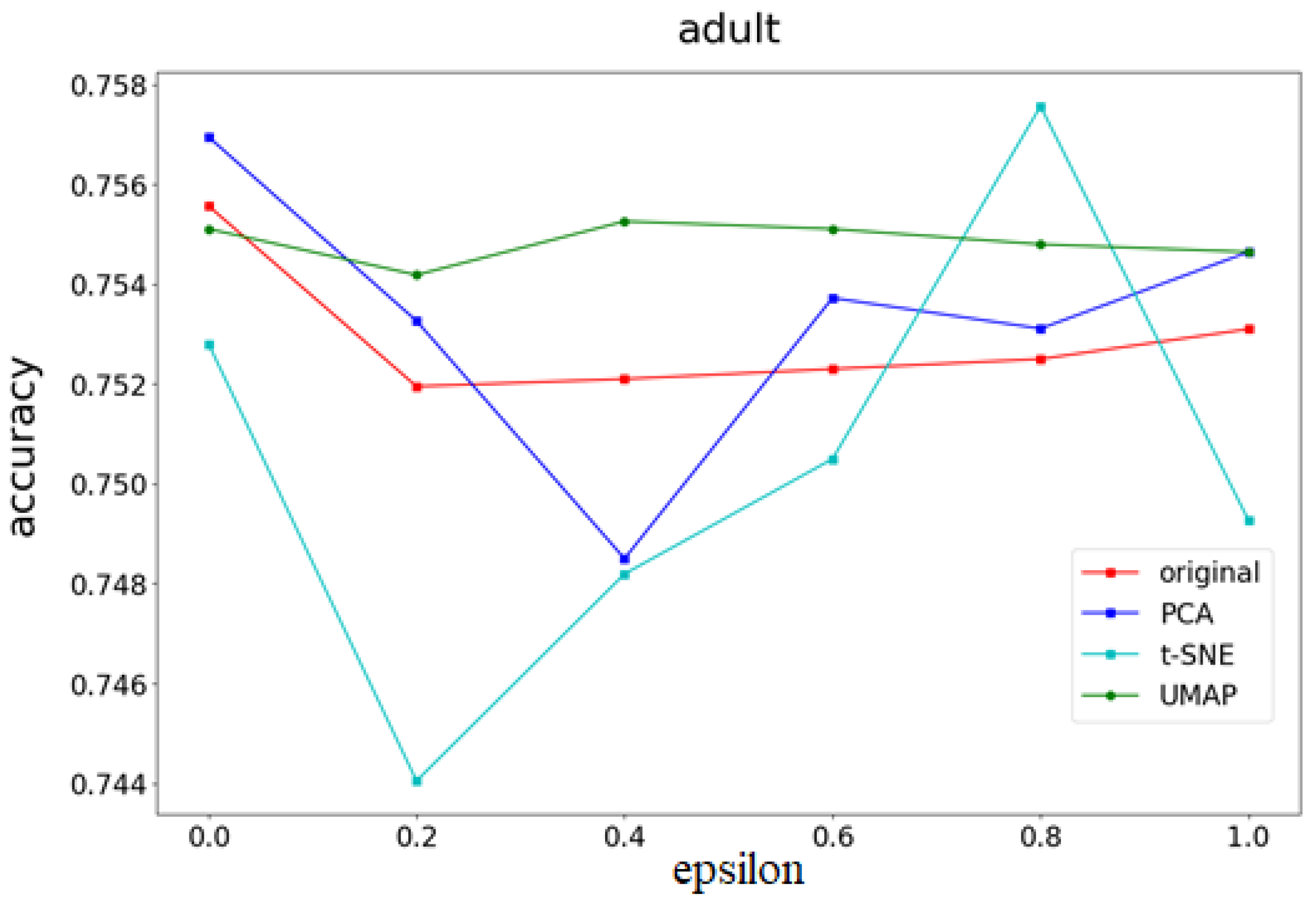
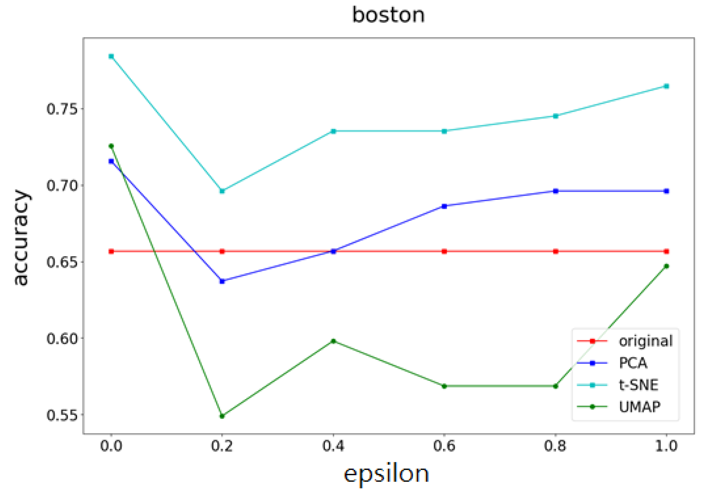
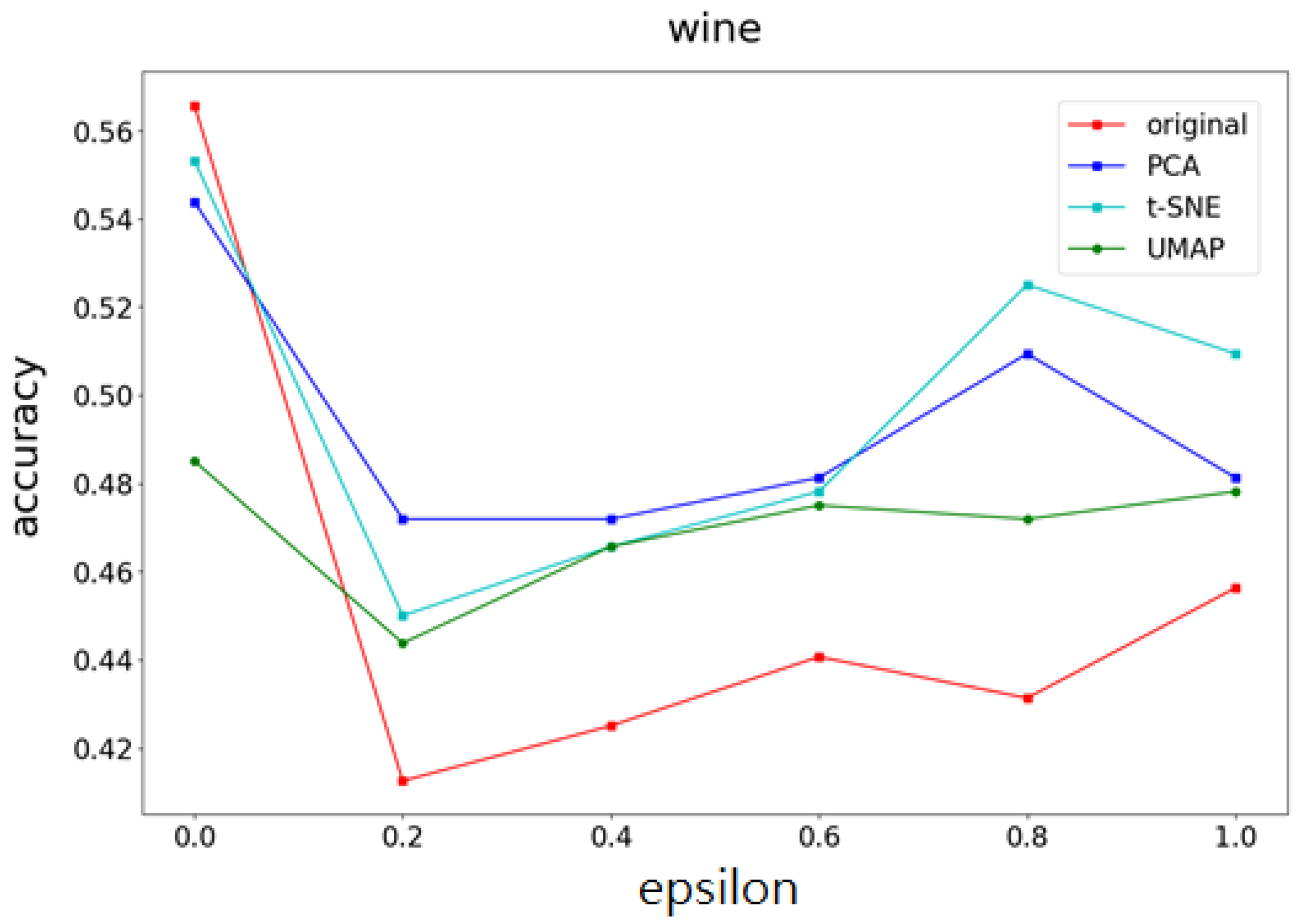
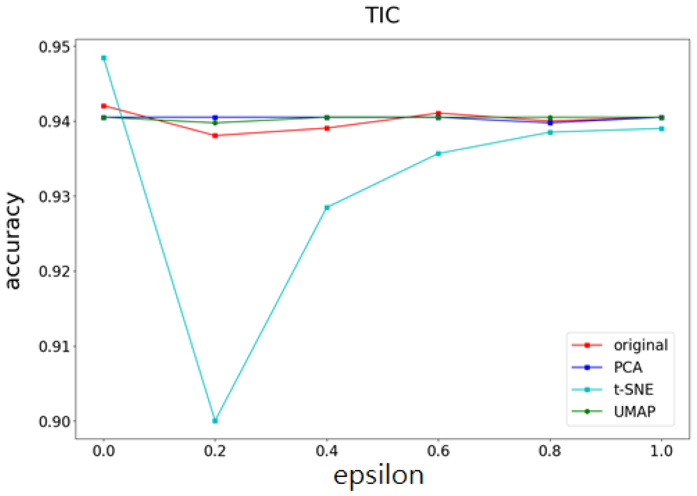
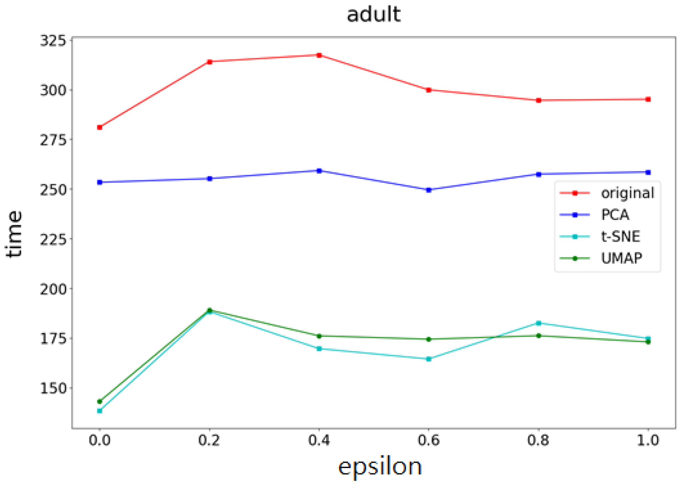
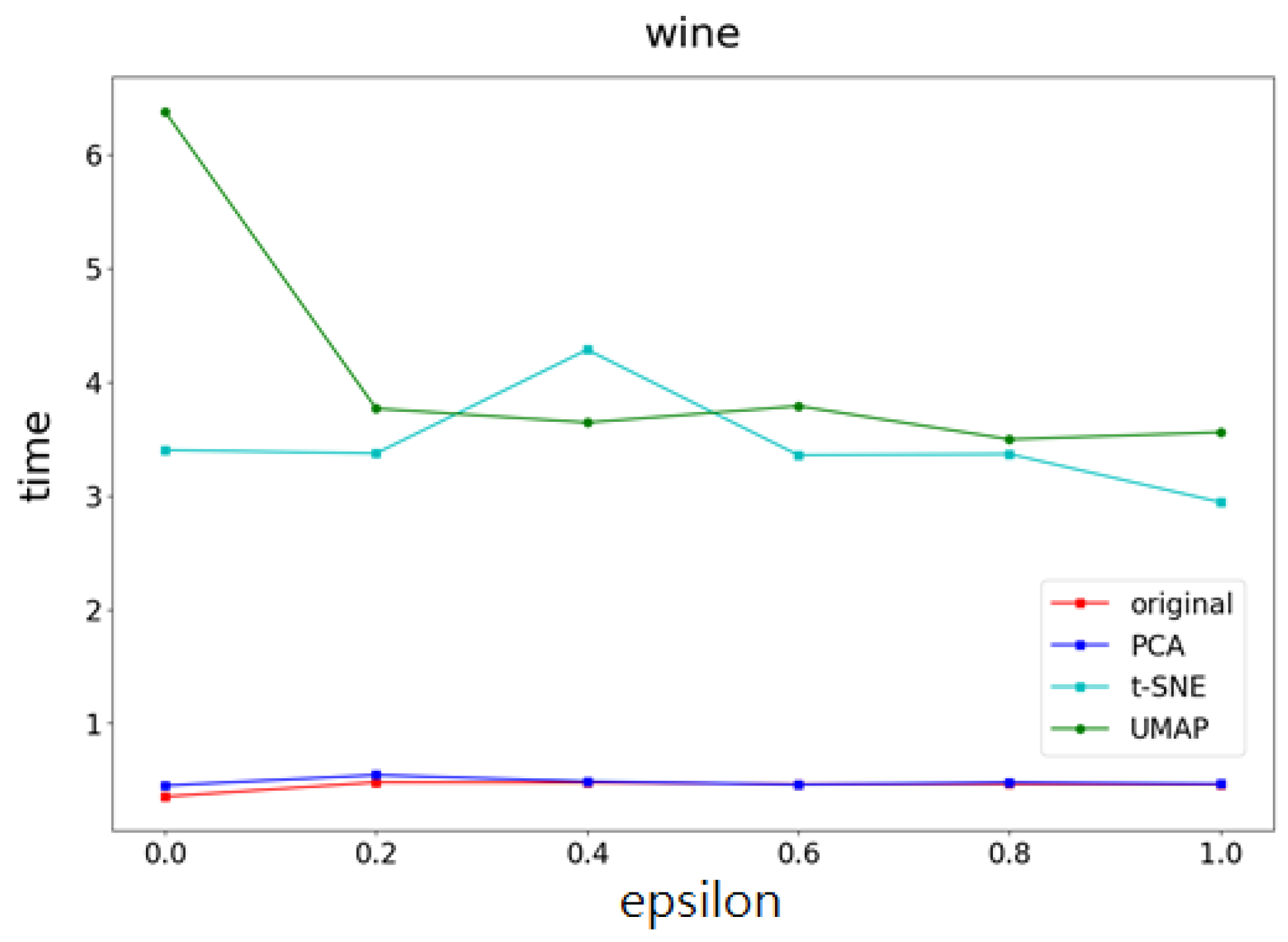
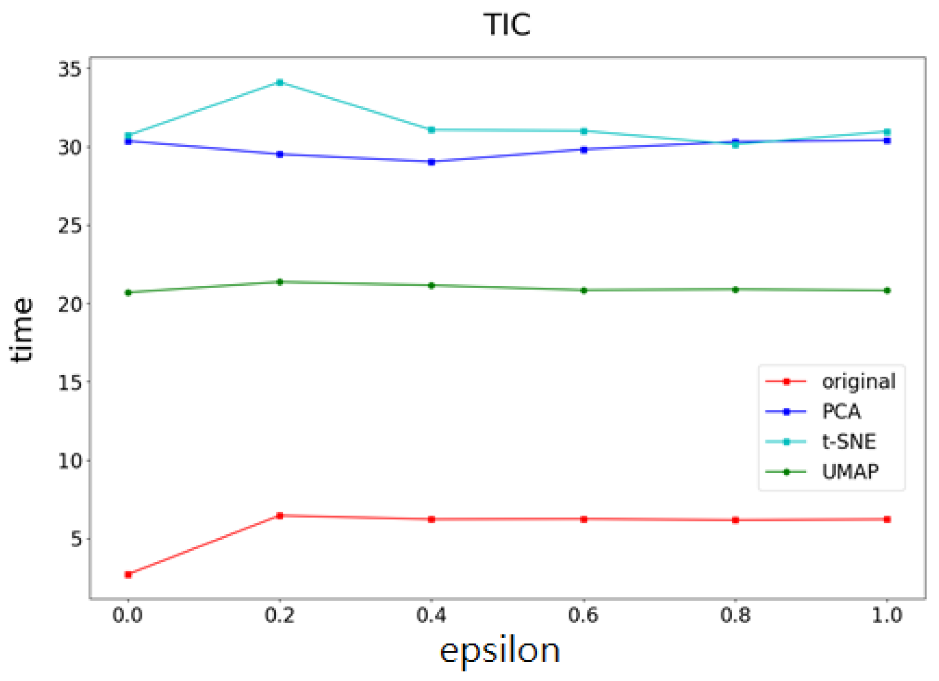
The accuracy and computational time of the privacy loss parameter ( ϵ ) are compared under the conditions of 0.2, 0.4, 0.6, 0.8, and 1. Epsilon ( ϵ ) is the core parameter of differential privacy, which is used to measure the risk of privacy leakage and provide a balance between privacy protection and data availability. Figure 3, Figure 4, Figure 5 and Figure 6 show the accuracy of the Adult, Boston, TIC, and Wine datasets, respectively. Figure 7, Figure 8, Figure 9 and Figure 10 show the computational time of the Adult, Boston, TIC, and Wine datasets, respectively. Table 3 and Table 4 summarize the accuracy and computational time of the average of the Adult, Boston, TIC, and Wine datasets.
Figure 3, Figure 4, Figure 5, Figure 6 show that the accuracy of the method using nonlinear dimensionality reduction (t-SNE) is higher than that of linear dimensionality reduction (PCA) in the Boston and Wine datasets. However, in the case of Adults with a larger number of data items and TIC with a large number of features, t-SNE performs worse than the PCA method. Figure 3 shows that the accuracy of the method using nonlinear dimensionality reduction (UMAP) is higher than that of others in the Case of Adults with a larger number of data items. Figure 6 shows that the accuracy of the method using t-SNE is lower than that of others in the case of TIC with a larger number of features. Under the number of features, it can be found that the accuracy is more affected by noise. The data after feature screening and extraction, along with their accuracy, are higher than the original dataset. Under the three methods and at the same feature scale, the scale and structure of the dataset have a significant impact on accuracy and calculation time. In terms of the scale of the dataset, it can be observed that the accuracy of the dataset with a larger data scale is more affected by noise than that of the dataset with a smaller number of data items.
From Figure 7, Figure 8, Figure 9, Figure 10 it is evident that the computational time of the method using nonlinear dimensionality reduction (t-SNE and UMAP) is higher than that of linear dimensionality reduction (PCA) in both the Boston and Wine datasets. However, in the case of Adults with a larger number of data items and TIC with a large number of features, UMAP performs worse than the PCA method. Under the number of data records, it can be found that the computational time of the Adult dataset with a larger number of data items is more affected by noise. The data after feature screening and extraction, along with their calculation speed, are faster than the original dataset.
In terms of calculation time, the dataset with a larger data scale has a more outstanding effect in reducing the calculation time. For example, the time spent on linear dimensionality reduction (PCA) for the Adult dataset with a larger number of data items is approximately 250 ms. When nonlinear dimensionality reduction methods (t-SNE and UMAP) are employed, the calculation time is significantly reduced to approximately 175 ms, and the calculation time of the UMAP method is faster than that of t-SNE (Figure 7). However, datasets with smaller data sizes are not suitable for nonlinear dimensionality reduction. For example, the datasets Boston (Figure 8) and Wine (Figure 9) are too small, and the calculation of nonlinear dimensionality reduction is more complicated. Therefore, the calculation time of nonlinear dimensionality reduction will be significantly increased.
Table 3 shows that the accuracy of t-SNE and PCA methods is highest than that of others. Table 4 shows that the computational times of the UMAP and t-SNE methods are superior to those of the others. In summary, t-SNE is the best feature extraction method for dimensionality reduction.
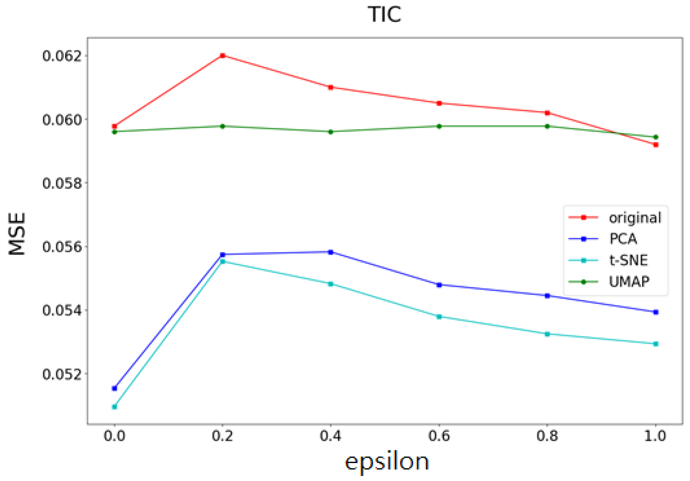
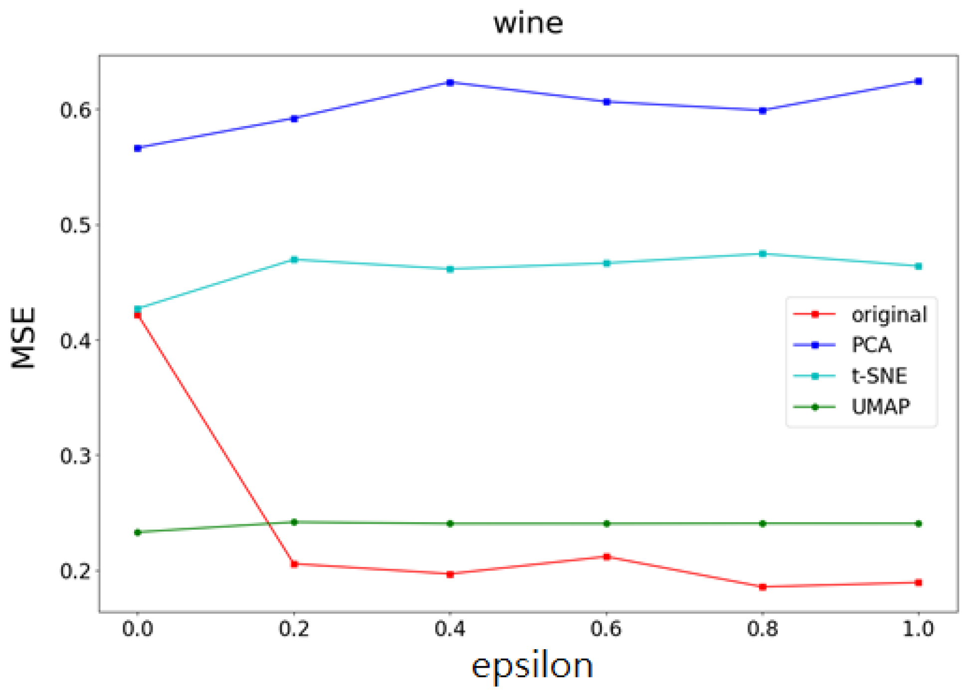
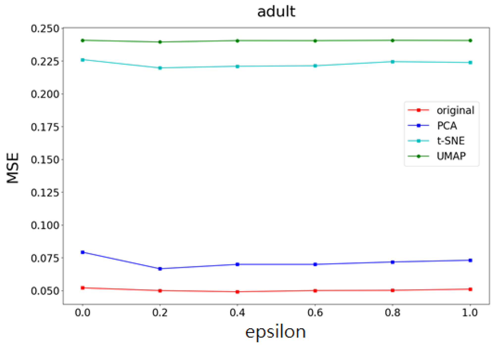
This experiment utilizes the mean square error (MSE) to evaluate the classification quality of each dimensionality reduction method across different datasets. The experimental results show that the MSE of the nonlinear dimensionality reduction (t-SNE) is superior (lowest) to that of others, as illustrated in Figure 11. In the classification quality of the Boston, Wine, and Adult datasets, which have a small number of features (as shown in Table 1, Figure 12, Figure 13, Figure 14), the original method yields the best MSE. Figure 14 shows that the MSE of the nonlinear dimensionality reduction (t-SNE and UMAP) is worse than that of the original and linear dimensionality reduction (t-SNE and UMAP) in the Adult dataset with a larger number of data items. This phenomenon may be due to the data distribution problem of the dataset. Nonlinear dimensionality reduction (t-SNE and UMAP) is too concerned about the local data structure when reducing the dimensionality, so it is easy to over-process the dataset, resulting in a decrease in its classification quality. It is important to note that MSE and accuracy may diverge due to the different aspects they measure. While accuracy reflects the proportion of correctly classified instances, MSE quantifies the overall prediction error, being sensitive to the magnitude of misclassification. Nonlinear dimensionality reduction methods, such as t-SNE and UMAP, emphasize preserving local data structures, which can distort the global data distribution. As a result, these methods may improve classification accuracy by better separating classes in high-dimensional space. Still, they may also produce a higher MSE if the predicted values deviate more from the actual values. Conversely, linear methods or the original dataset may retain more of the global data structure, leading to lower MSE but not necessarily the highest accuracy. This divergence highlights that both metrics provide complementary perspectives on model performance, and considering them together offers a more comprehensive evaluation of dimensionality reduction methods in differentially private machine learning.
This study combines feature importance with UMAP, t-SNE, and PCA to propose a method for improving the performance of differentially private data in machine learning. The method consists of two parts:
  • Part I Calculates the correlation of the data feature importance set, then sequentially removes features with low importance and high correlation to find the optimal number of features.
  • Part II Dimensionality reduction is performed using multiple UMAP, t-SNE, and PCA methods, respectively, and weights are determined based on the feature importances calculated in Part I. After obtaining the weighting parameters, noise is added. This method effectively reduces the added noise, preventing excessive noise from being introduced into the data, thereby minimizing its impact on machine learning performance.
In addition to accuracy and computational time, this study also investigates the geometric “symmetry” preserved by different dimensionality reduction methods. Here, symmetry is defined as the extent to which the pairwise distance distribution and neighborhood structure of the original high-dimensional data are preserved after dimensionality reduction. We use the structural symmetry score as a quantitative measure, which is calculated based on the proportion of preserved k = 3 -nearest neighbors.
The results indicate that t-SNE better preserves local neighborhood structures, as evidenced by higher structural symmetry scores in the Boston and Wine datasets. In contrast, PCA exhibits stronger performance in preserving global distance distributions (higher distributional symmetry in TIC). This substantiates the claim that t-SNE is more effective at maintaining local geometric symmetry, whereas PCA tends to preserve global linear relationships.

4.4. The Optimality

The goal of the proposed privacy-preserving model is to maximize model accuracy while minimizing the risk of privacy leakage, as determined by the differential privacy parameter ϵ . Formally, the optimization problem can be expressed as follows:
max M U ( M ) λ · L ( M , ϵ ) ,
where M denotes the proposed model with dimensionality reduction, U ( M ) denotes the accuracy, L ( M , ϵ ) denotes the privacy leakage loss function, and λ is a balancing coefficient.
In this subsection, we show that the proposed two-stage method (Part I: feature selection by importance; Part II: dimensionality reduction and weighted noise addition) yields an efficient solution within the aforementioned framework.
In Part I, by iteratively removing features with low importance and high correlation, we ensure that the retained features maximize information gain U ( M ) while minimizing redundancy.
In Part II, the dimensionality reduction step is equivalent to a projection onto a lower-dimensional manifold, where the noise scale is reduced proportionally to the retained feature importance weights. This guarantees that the Laplace or Gaussian mechanism introduces the minimum necessary perturbation.
Combining Part I and Part II, the objective function in Equation (1) is maximized because both the accuracy term is increased and the privacy loss term is decreased.
Thus, the proposed model achieves the optimal trade-off between accuracy and privacy leakage under the differential privacy constraint.

5. Conclusions and Discussion

This article proposes a method for optimizing machine learning performance based on differential privacy. It compares the accuracy and computational time of t-SNE, UMAP, and PCA in terms of feature importance. Experimental results show that linear dimensionality reduction methods such as PCA offer the advantage of fast dimensionality reduction. However, if the dataset is nonlinear, PCA dimensionality reduction can easily lead to data structure loss, resulting in data bias and affecting model accuracy. Therefore, this paper employs t-SNE, a nonlinear dimensionality reduction technique. t-SNE effectively avoids the data congestion and loss of data structure associated with linear dimensionality reduction. Compared to PCA, it offers higher accuracy and better visualization capabilities.
In terms of computational efficiency, Table 4 shows that UMAP achieves the fastest average runtime, followed closely by t-SNE, while PCA and the original datasets require more time. Thus, although t-SNE provides superior accuracy and visualization, UMAP demonstrates greater computational efficiency. Based on these findings, the proposed method of optimizing differentially private machine learning performance by combining feature importance with dimensionality reduction methods (particularly t-SNE for accuracy and UMAP for efficiency) can effectively improve both model accuracy and computational time.
The proposed framework demonstrates strong applicability in a variety of real-world scenarios that require balancing data privacy and practicality. In healthcare, federated learning enables hospitals to collaboratively train diagnostic or medical imaging models without sharing sensitive patient data, thereby improving model robustness while complying with privacy regulations. In finance, multiple institutions can jointly develop fraud detection or credit scoring systems under strict legal constraints (such as the General Data Protection Regulation (GDPR)), thereby improving accuracy without compromising data confidentiality. For consumer-facing services, federated learning has been widely adopted in mobile applications such as predictive text input, personalized recommendations, and speech recognition. By training models directly on user devices, companies can provide adaptive services while protecting user privacy. Furthermore, in industrial IoT and smart city applications, where a large number of distributed sensors generate data, the framework supports secure real-time analysis and anomaly detection. These examples illustrate the practical value of our approach across various fields and demonstrate its potential to address regulatory challenges and meet performance requirements in real-world deployments.

Author Contributions

N.-I.W. and J.-T.W. proposed the idea and wrote this paper; M.-S.H. discussed, supervised, and reviewed the methodology and manuscript; All authors have read and agreed to the published version of the manuscript.

Funding

The National Science and Technology Council partially supported this research, Taiwan (ROC), under contract no.: NSTC 113-2221-E-468-016 and NSTC 112-2221-E-468-007.

Data Availability Statement

The original contributions presented in this study are included in the article. Further inquiries can be directed to the corresponding author.

Conflicts of Interest

The authors declare no conflicts of interest.

References

  1. Cuzzocrea, A. Privacy-Preserving Big Data Stream Mining: Opportunities, Challenges, Directions. In Proceedings of the 2017 IEEE International Conference on Data Mining Workshops, New Orleans, LA, USA, 18–21 November 2017. [Google Scholar] [CrossRef]
  2. Council of the European Union. 2016. General Data Protection Regulation. Available online: https://gdpr-info.eu/ (accessed on 7 September 2025).
  3. Cao, J.; Ren, J.; Guan, F.; Li, X.; Wang, N. K-anonymous Privacy Protection Based on You Only Look Once Network and Random Forest for Sports Data Security Analysis. Int. J. Netw. Secur. 2025, 27, 264–273. [Google Scholar]
  4. Mothukuri, V.; Parizi, R.M.; Pouriyeh, S.; Huang, Y.; Dehghantanha, A.; Srivastava, G. A Survey on Security and Privacy of Federated Learning. Future Gener. Comput. Syst. 2021, 115, 619–640. [Google Scholar] [CrossRef]
  5. Chen, J.; Gong, L.; Chen, J. Privacy Preserving Scheme in Mobile Edge Crowdsensing Based on Federated Learning. Int. J. Netw. Secur. 2024, 26, 74–83. [Google Scholar]
  6. Li, Q.; Wen, Z.; He, B. Federated Learning Systems: Vision, Hype and Reality for Data Privacy and Protection. arXiv 2019, arXiv:1907.09693. [Google Scholar] [CrossRef]
  7. Li, T.; Sahu, A.K.; Talwalkar, A.; Smith, V. Federated Learning: Challenges, Methods, and Future Directions. IEEE Signal Process 2019, 37, 50–60. [Google Scholar] [CrossRef]
  8. Hard, A.; Rao, K.; Mathews, R.; Ramaswamy, S.; Beaufays, F.; Augenstein, S.; Eichner, H.; Kiddon, C.; Ramage, D. Federated Learning for Mobile Keyboard Prediction. arXiv 2019, arXiv:1811.03604v2. Available online: https://arxiv.org/pdf/1811.03604.pdf (accessed on 21 July 2025). [CrossRef]
  9. Xu, N.; Feng, T.; Zheng, J. Ice-snow Physical Data Privacy Protection Based on Deep Autoencoder and Federated Learning. Int. J. Netw. Secur. 2025, 27, 314–322. [Google Scholar]
  10. Yu, J.; Huang, L.; Zhao, L. Art Design Data Privacy Protection Strategy Based on Blockchain Federated Learning and Long Short-term Memory. Int. J. Netw. Secur. 2024, 26, 573–581. [Google Scholar]
  11. Hu, W.P.; Lin, C.B.; Wu, J.T.; Yang, C.Y.; Hwang, M.S. Research on Privacy and Security of Federated Learning in Intelligent Plant Factory Systems. Int. J. Netw. Secur. 2023, 25, 377–384. [Google Scholar]
  12. Lin, J.; Du, M.; Liu, J. Free-Riders in Federated Learning: Attacks and Defenses. arXiv 2019, arXiv:1911.12560. Available online: https://api.semanticscholar.org/CorpusID:208513099 (accessed on 21 July 2025). [CrossRef]
  13. Chen, J.; Zhang, J.; Zhao, Y.; Han, H.; Zhu, K.; Chen, B. Beyond Model-Level Membership Privacy Leakage: An Adversarial Approach in Federated Learning. In Proceedings of the 29th International Conference on Computer Communications and Networks (ICCCN), Honolulu, HI, USA, 3–6 August 2020. [Google Scholar]
  14. Li, X.G.; Li, H.; Li, F.; Zhu, H. A Survey on Differential Privacy. J. Cyber Secur. 2018, 3, 92–104. [Google Scholar]
  15. Ji, Z.; Lipton, Z.C.; Elkan, C. Differential Privacy and Machine Learning: A Survey and Review. arXiv 2014, arXiv:1412.7584. Available online: https://arxiv.org/abs/1412.7584 (accessed on 21 July 2025). [CrossRef]
  16. Dong, W.; Sun, D.; Yi, K. Better than Composition: How to Answer Multiple Relational Queries under Differential Privacy. Proc. ACM Manag. Data 2023, 1, 1–26. [Google Scholar] [CrossRef]
  17. Laouir, A.E.; Imine, A. Private Approximate Query over Horizontal Data Federation. arXiv 2024, arXiv:2406.11421. Available online: https://arxiv.org/abs/2406.11421 (accessed on 21 July 2025).
  18. Abadi, M.; Chu, A.; Goodfellow, I.; McMahan, H.B.; Mironov, I.; Talwar, K.; Zhang, L. Deep Learning with Differential Privacy. In Proceedings of the 2016 ACM SIGSAC Conference on Computer and Communications Security, Vienna, Austria, 24–28 October 2016; pp. 308–318. [Google Scholar]
  19. Ni, L.; Li, C.; Wang, X.; Jiang, H.; Yu, J. DP-MCDBSCAN: Differential Privacy Preserving Multi-Core DBSCAN Clustering for Network User Data. IEEE Access 2018, 6, 21053–21063. [Google Scholar] [CrossRef]
  20. Wang, J.; Wang, A. An Improved Collaborative Filtering Recommendation Algorithm Based on Differential Privacy. In Proceedings of the IEEE 11th International Conference on Software Engineering and Service Science (ICSESS), Beijing, China, 16–18 October 2020; pp. 310–315. [Google Scholar]
  21. Sharma, J.; Kim, D.; Lee, A.; Seo, D. On Differential Privacy-Based Framework for Enhancing User Data Privacy in Mobile Edge Computing Environment. IEEE Access 2021, 9, 38107–38118. [Google Scholar] [CrossRef]
  22. Ji, Z.; Elkan, C. Differential privacy based on importance weighting. Mach. Learn. 2013, 93, 163–183. [Google Scholar] [CrossRef] [PubMed]
  23. Akmeşe, Ö.F. A novel random number generator and its application in sound encryption based on a fractional-order chaotic system. J. Circuits Syst. Comput. 2023, 32, 2350127. [Google Scholar] [CrossRef]
  24. Akmeşe, Ö.F. Data privacy-aware machine learning approach in pancreatic cancer diagnosis. BMC Med. Inform. Decis. Mak. 2024, 24, 248. [Google Scholar] [CrossRef]
  25. Alaca, Y.; Akmeşe, Ö.F. Pancreatic Tumor Detection from CT Images Converted to Graphs Using Whale Optimization and Classification Algorithms with Transfer Learning. Int. J. Imaging Syst. Technol. 2025, 35, e70040. [Google Scholar] [CrossRef]
  26. Tozlu, B.H.; Akmeşe, Ö.F.; Şimşek, C.; Şenel, E. A New Diagnosing Method for Psoriasis from Exhaled Breath. IEEE Access 2025, 13, 25163–25174. [Google Scholar] [CrossRef]
  27. Li, W.; Zhang, X.; Li, X.; Cao, G.; Zhang, Q. PPDP-PCAO: An Efficient High-Dimensional Data Releasing Method with Differential Privacy Protection. IEEE Access 2019, 7, 176429–176437. [Google Scholar] [CrossRef]
  28. Maaten, L.V.D.; Hinton, G. Visualizing Data using t-SNE. J. Mach. Learn. 2008, 9, 2579–2605. [Google Scholar]
  29. McInnes, L.; Healy, J.; Melville, J. UMAP: Uniform Manifold Approximation and Projection for Dimension Reduction. arXiv 2018, arXiv:1802.03426. [Google Scholar] [CrossRef]
  30. Becker, B.; Kohavi, R.; Adult Data Set. UCI Machine Learning Repository. 1996. Available online: https://archive.ics.uci.edu/ml/datasets/adult (accessed on 21 July 2025).
  31. Harrison, D.; Rubinfeld, D.L. Hedonic housing prices and the demand for clean air. J. Environ. Econ. Manag. 1978, 5, 81–102. [Google Scholar] [CrossRef]
  32. Sentient Machine Research. TIC Data Set (CARAVAN Insurance Challenge) UCI Machine Learning Repository. Available online: https://www.kaggle.com/datasets/uciml/caravan-insurance-challenge (accessed on 7 September 2025).
  33. Cortez, P.; Cerdeira, A.; Almeida, F.; Matos, T.; Reis, J. Modeling wine preferences by data mining from physicochemical properties. Decis. Support Syst. 2009, 47, 547–553. [Google Scholar] [CrossRef]
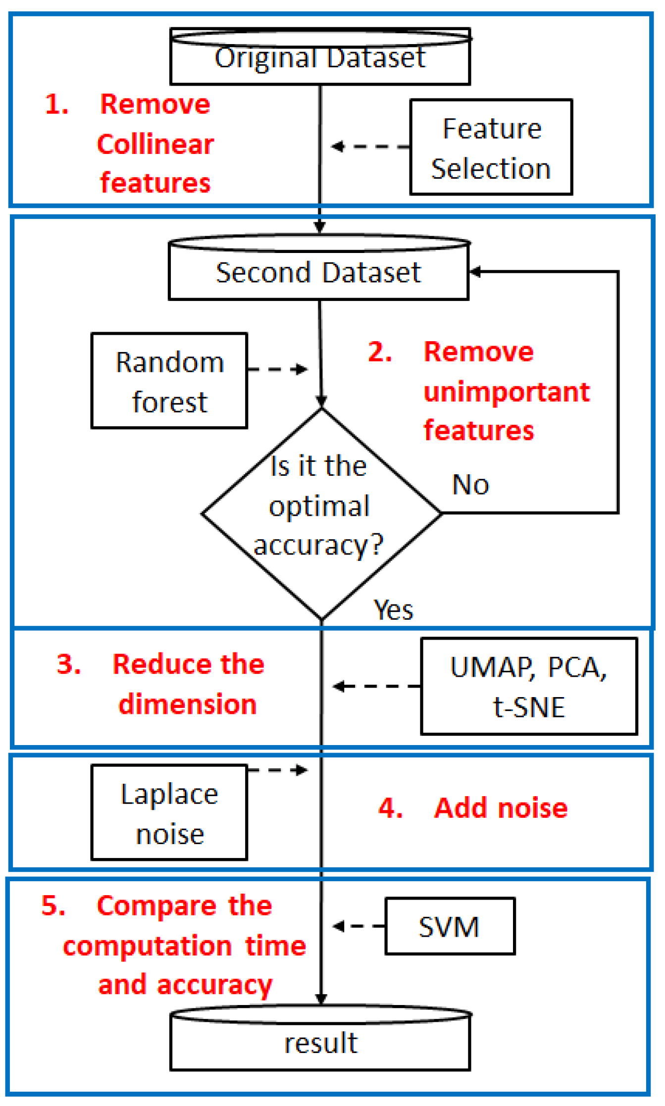
Figure 1. The process architecture of this study.
Symmetry 17 01747 g001
Figure 3. The accuracy of the Adult dataset.
Symmetry 17 01747 g003
Figure 4. The accuracy of the Boston dataset.
Symmetry 17 01747 g004
Figure 5. The accuracy of the Wine dataset.
Symmetry 17 01747 g005
Figure 6. The accuracy of the TIC dataset.
Symmetry 17 01747 g006
Figure 7. The computational time of the Adult dataset.
Symmetry 17 01747 g007
Figure 8. The computational time of the Boston dataset.
Symmetry 17 01747 g008
Figure 9. The computational time of the Wine dataset.
Symmetry 17 01747 g009
Figure 10. The computational time of the TIC dataset.
Symmetry 17 01747 g010
Figure 11. The MSE of the TIC dataset.
Symmetry 17 01747 g011
Figure 12. The MSE of the Boston dataset.
Symmetry 17 01747 g012
Figure 13. The MSE of the Wine dataset.
Symmetry 17 01747 g013
Figure 14. The MSE of the Adult dataset.
Symmetry 17 01747 g014
Table 2. Experimental reproducibility settings.
ComponentHyperparameters
SVMkernel = ‘rbf’; gamma = ‘scale’; random_state = 42
Random Seed42 (applied across all methods)
Librariesscikit-learn 1.5.2
Table 3. The accuracy of the average of Adult, Boston, TIC, and Wine datasets.
Accuracy ϵ = 0.2 ϵ = 0.4 ϵ = 0.6 ϵ = 0.8 ϵ = 1.0 Average
Original0.68880.69400.69750.69570.69970.6951
PCA0.70180.70360.71380.72560.71630.7122
t-SNE0.69850.72050.72530.74260.74060.7255
UMAP0.67230.69030.68370.68280.70240.6863
Table 4. The computational time of the average of Adult, Boston, TIC, and Wine datasets.
Computational Time ϵ = 0.2 ϵ = 0.4 ϵ = 0.6 ϵ = 0.8 ϵ = 1.0 Average
Original80.3880.8476.8175.7975.7877.92
PCA71.4072.5170.1473.3074.1672.30
t-SNE55.4752.1950.0953.7152.7452.84
UMAP52.4050.1249.6349.5949.3550.22
Disclaimer/Publisher’s Note: The statements, opinions and data contained in all publications are solely those of the individual author(s) and contributor(s) and not of MDPI and/or the editor(s). MDPI and/or the editor(s) disclaim responsibility for any injury to people or property resulting from any ideas, methods, instructions or products referred to in the content.