Article

MiT-WGAN: Financial Time-Series Generation GAN Based on Multi-Convolution Dynamic Fusion and iTransformer

School of Electronic Information Engineering, Guiyang University, Guiyang 550005, China
*
Author to whom correspondence should be addressed.
Symmetry 2025, 17(10), 1740; https://doi.org/10.3390/sym17101740
Submission received: 29 August 2025 / Revised: 2 October 2025 / Accepted: 7 October 2025 / Published: 15 October 2025
(This article belongs to the Section Mathematics)

Abstract

With the rapid growth of FinTech, time-series data has become pervasive in financial markets. However, the nonstationarity, high noise levels, and complex temporal dependencies of financial data pose significant challenges to the efficacy and stability of standard generative models. To overcome these limitations, we propose MiT-WGAN, a gradient-penalized Wasserstein generative adversarial network that integrates a multi-convolutional dynamic fusion (MCDF) module in parallel with an enhanced Transformer (iTransformer) to jointly capture local patterns and long-range dependencies. We evaluate MiT-WGAN on S&P 500 stock trading data using a comprehensive set of baseline models and evaluation metrics. Experimental results demonstrate that MiT-WGAN achieves superior sample quality, better preservation of statistical properties, and improved training stability, confirming its effectiveness for financial time-series modeling.

1. Introduction

Driven by the digital economy, financial markets generate large volumes of time-series data, including high-frequency trading records, market microstructure indicators, and macroeconomic measures. These data have become a pivotal resource for intelligent finance [1,2], as they reflect market dynamics and support forecasting, risk management, and investment decisions. In applications such as credit risk assessment [3], asset allocation [4], and financial regulation [5], time-series modeling and analysis have become core technologies for enhancing the resilience of the financial system.
Compared with more common sensory modalities such as images and speech, the acquisition of financial time-series data is constrained by privacy concerns, trade secrets, and regulatory policies, which complicates the collection of large, diverse, high-quality datasets [6]. Moreover, black-swan events and structural market changes [7] further hinder the learning and generalization ability of deep learning models, especially when training data are limited. Consequently, the use of generative models to synthesize high-quality virtual data has emerged as an effective approach to mitigate data scarcity and to improve model performance under extreme scenarios [8,9].
In recent years, generative adversarial networks (GANs) [10] have shown considerable promise for time-series generation. The adversarial training paradigm has been demonstrated to improve the realism and diversity of generated samples, with applications in areas such as financial fraud detection [11], portfolio optimization [12], and market forecasting [13]. Nonetheless, owing to stylized features of financial time series—including high noise, nonlinear dynamics, and volatility clustering—conventional GAN architectures built on multilayer perceptrons or recurrent neural networks struggle to capture cross-scale dynamic dependencies [14].
To overcome these limitations, researchers have adopted architectures that combine local-feature extractors and long-range dependency models, e.g., convolutional neural networks (CNNs) for local patterns [15,16] and Transformers for long-range dependencies [17,18]. Two main shortcomings remain. First, it remains challenging to integrate local features and global temporal dependencies in an organic manner, especially when fine-grained signals and macro trends coexist in financial time series. Second, many fusion strategies rely on simple concatenation or fixed weighting of features, lacking dynamic, adaptive mechanisms and thus failing to adapt to rapid market fluctuations and structural shifts.
Motivated by these observations, this study proposes MiT-WGAN, an improved generative architecture that places a multi-convolutional dynamic fusion (MCDF) module and an iTransformer in parallel and adaptively fuses their outputs via a dynamic gated feature-fusion module. The MCDF module extracts features in parallel across multiple convolutional kernel sizes and uses attention to adaptively weight and select appropriate feature representations [19]. The iTransformer reorients the input representation from the temporal dimension to the variable dimension, enabling modeling of long-range dependencies and inter-variable interactions while alleviating the computational redundancy of standard Transformers on long sequences [20]. Thus, the combined architecture captures both multi-scale local temporal patterns and long-range cross-variable dependencies.
Finally, traditional GANs often suffer from mode collapse and training instability—problems that are exacerbated when processing noisy financial time-series data [21]. To improve training stability and convergence, this study adopts the Wasserstein GAN with gradient penalty (WGAN-GP) [22].
The contributions of this paper are summarized as follows:
  • The present study proposes MiT-WGAN, a hybrid generative adversarial framework for financial time-series generation. In contrast to extant methodologies that depend exclusively on a solitary feature extraction mechanism (e.g., QuantGAN based on TCN, TimeGAN relying on supervised embedding, and diffusion models using stepwise denoising generation), this study integrates multi-convolutional dynamic fusion (MCDF) with an enhanced Transformer (iTransformer) to concurrently model local multi-scale patterns and long-term temporal dependencies.
  • The dynamic gated fusion (DGF) mechanism is introduced to achieve an adaptive balance between local and global features. In contrast to conventional methods such as simple splicing or static weighting, DGF employs a learnable gating unit to adaptively adjust the contribution ratio of the MCDF and iTransformer branches based on the characteristics of the data. This enhances the model’s robustness and its capacity for generalization in nonstationary financial sequences.
  • To mitigate instability, vanishing gradients, and mode collapse commonly encountered in GAN training on noisy financial time series, the adversarial framework adopts the Wasserstein GAN with gradient penalty (WGAN-GP), which stabilizes training and improves generator convergence.
  • We evaluate MiT-WGAN on two stock datasets sampled from the S&P 500 and compare its performance against several state-of-the-art time-series generative models. Using multiple quantitative metrics, the experiments demonstrate that MiT-WGAN significantly outperforms baseline methods in modeling logarithmic returns of financial time series.
The remainder of this paper is organized as follows. Section 2 reviews the existing literature on time-series data generation, with an emphasis on recent advances in the generation of financial time series. Section 3 presents MiT-WGAN, the novel method proposed in this study, and provides a detailed description of its design, model background, and theoretical foundations. Section 4 describes the experimental setup and presents a thorough analysis of the results. Section 5 concludes the paper with a concise summary of the findings and suggestions for future research.

2. Related Work

2.1. Time-Series GAN

Recent years have seen increasing application of generative adversarial networks (GANs) to the modeling and generation of time-series data, particularly for mitigating data scarcity and improving sample quality. Building on the standard GAN framework, researchers have incorporated sequence-modeling mechanisms to better capture temporal dynamics. TimeGAN [8] combines autoencoders with adversarial learning to enhance temporal dependency modeling through reconstruction and supervised losses. C-RNN-GAN [23] employs recurrent neural networks (RNNs) for progressive generation of continuous sequences, demonstrating strong performance in speech and music generation tasks. SeqGAN [24] addresses the challenge of learning with discrete sequences by adopting policy-gradient optimization, thereby extending GAN applicability to discrete domains such as natural language and symbolic sequences.
However, the majority of these methods are predicated on a solitary modeling framework (RNN or embedding mechanism), a factor that hinders the capacity to capture long-term dependencies while concurrently preserving the characterization of local fluctuation patterns. Moreover, the pervasive instability inherent in the training of GANs imposes constraints on the model’s capacity to generalize to intricate time-series data.
The conditional generative adversarial network (CGAN) extends the standard GAN by conditioning both the generator and discriminator on external information, which enhances controllability over the generation process [25]. COT-GAN [26] is based on a causal optimal transmission mechanism and uses temporal positions and contextual information as conditional inputs, improving the dynamic consistency between generated samples and real sequences. RCGAN [14] addresses missing values in medical time series by conditioning an RNN generator on auxiliary information, outperforming traditional interpolation methods in health-data simulation. Nevertheless, CGAN and its extensions are predicated on strong prior assumptions in conditional construction. In instances where conditional variables prove to be inadequate or exhibit excessive noise, there is a substantial decline in the efficacy of model generation.

2.2. Financial Time-Series GAN

GANs have also shown structural advantages for generating financial time series. QuantGAN [27] integrates temporal convolutional networks (TCNs) within an adversarial framework to model log-returns, improving the simulation of market volatility. Fin-GAN [28] reproduces key stylized facts of financial time series—including linear unpredictability, fat-tailed distributions, volatility clustering, leverage effects, multi-scale volatility correlations, and asymmetric price fluctuations—thereby enhancing adaptability and accuracy in complex market scenarios. RSQGAN [29] employs the Greedy Gaussian Segmentation (GGS) algorithm to partition market regimes (e.g., normal vs. crisis) and integrates a conditional GAN with TCNs to generate log-return series under different market conditions, improving generation quality in extreme scenarios.
While extant methodologies have demonstrated efficacy in capturing the stylized facts of financial sequences, the majority of models continue to prioritize a singular architectural framework (e.g., pure convolution or conditional segmentation). This limitation impedes their capacity to collaboratively model multi-scale local features and global long-term dependencies. Additionally, the efficacy of these methods in highly volatile and nonstationary market environments is yet to be optimized.

2.3. Methods Based on VAE and Diffusion Model

Beyond GANs, variational autoencoders (VAEs) have been widely applied to time-series generation. Recent work indicates that modeling latent variables at the sequence level can capture both short- and long-term dependencies and thus improve generation quality [30,31]. However, typical VAE-type models frequently generate series that are excessively smooth, and they are often incapable of replicating the substantial fluctuations and fat-tailed distribution characteristics that are frequently observed in financial time series.
Diffusion models have also achieved strong results in generative tasks; their progressive denoising mechanism is well suited to time-series modeling. TimeGrad employs an autoregressive denoising diffusion process for probabilistic forecasting of multivariate time series, enhancing diversity while preserving statistical properties [32]. Subsequent studies developed unconditional/self-guided diffusion modeling and inference strategies for time series [33]. A recent review systematically summarizes progress and advantages of diffusion models in time-series forecasting [34]. However, diffusion models frequently necessitate substantial computational resources and exhibit sluggish generation rates, rendering them impractical for financial scenarios that demand efficient modeling.
A survey of extant research reveals a broad array of methodologies, ranging from early recurrent neural network (RNN) and convolutional neural network (CNN) models to more recent causal optimal transfer methods (e.g., COT-GAN) and diffusion models (e.g., TimeGrad). These approaches have been demonstrated to exhibit strengths in dynamic consistency, probabilistic modeling, and distribution fitting, respectively. However, these methods are not without their limitations. These include the difficulty of simultaneously modeling local and global features, overly smooth generated sequences, and computational inefficiency. In contrast, the MiT-WGAN proposed in this paper emphasizes the fusion of convolution and Transformer networks, with the objective of simultaneously capturing local patterns and long-term dependencies in financial time series. Consequently, this research not only maintains close ties with recent generative models but also complements them methodologically, thereby laying the foundation for further systematic comparisons of different paradigms.

3. Methodology

3.1. GAN

The Generative Adversarial Network (GAN), proposed by Goodfellow et al. [10], belongs to a class of generative models. A GAN is trained to map random noise into synthetic samples that closely resemble real data. It consists of two neural networks: a generator and a discriminator.
Let z R N z denote a random noise vector, and let G denote the generator. The generator is a parameterized function defined as
G : R N z × Θ ( G ) R N z ,
where Θ ( G ) denotes the parameter space of G (e.g., weights and biases). The generated sample is therefore
x ˜ = G ( z ; θ ( G ) ) R N x ,
Let x R N x be a real data sequence. Let θ ( D ) Θ ( D ) denote the discriminator’s learnable parameters, and let σ : R [ 0 , 1 ] be the sigmoid function defined by σ ( t ) = 1 / ( 1 + e t ) . The discriminator is a parameterized function:
D : R N x × Θ ( D ) [ 0 , 1 ] ,
typically implemented as a neural network whose output can be written as D ( x ; θ ( D ) ) = σ ( f ( x ; θ ( D ) ) ) , where f denotes the network’s pre-activation output [27].
Training a standard GAN is formulated as a two-player minimax game. The generator aims to fool the discriminator by producing samples whose distribution matches that of the real data, while the discriminator seeks to distinguish real from generated samples. Formally, the game is written as
min G max D V ( D , G ) = E x p data ( x ) [ log D ( x ) ] + E z p z ( z ) [ log ( 1 D ( G ( z ) ) ) ] ,

3.2. MiT-WGAN

The overall architecture of MiT-WGAN is illustrated in Figure 1. MiT-WGAN comprises two modules: a generator and a discriminator. The generator produces financial logarithmic returns, while the discriminator evaluates their authenticity.
Within the generator, a noise vector z R N z sampled from a Gaussian distribution (e.g., z N ( 0 , I ) ) is used as input, where N z is a tunable hyperparameter. The input is processed in parallel by the multi-convolutional dynamic fusion (MCDF) module and the iTransformer.
The outputs of these two modules are fused by a dynamic gated feature-fusion (DGF) module and then passed through a t a n h activation to produce the generated series x g e n R T × N x . The discriminator receives either x g e n or the real log-return series x r e a l R T × N x as input. The discriminator’s backbone mirrors the generator’s architecture; however, after the DGF module, the discriminator applies global average pooling (instead of a t a n h activation) to produce a scalar real-valued score that is used for loss computation (consistent with the WGAN-GP training objective).

3.2.1. Multi-Convolution Dynamic Fusion

Convolutional neural networks (CNNs) are widely used for time-series modeling because of their strong local feature-extraction capabilities. Convolutional operations often outperform recurrent neural networks (RNNs) in capturing local dependencies and enabling parallel computation, which is particularly advantageous when processing data that exhibit local patterns and abrupt changes, such as financial time series [15,16]. However, a single convolutional kernel often fails to capture features at multiple temporal scales. To address this limitation, multi-scale convolutional architectures have been proposed: extracting features in parallel with multiple convolutional kernels allows the model to capture patterns across different receptive fields.
The multi-convolution dynamic fusion (MCDF) module used in this study is shown in Figure 2. Given an input sequence—noise for the generator or real/generated log-returns for the discriminator—the data are processed by k parallel one-dimensional (1-D) convolutional branches ( C o n v 1 , C o n v 2 , · , C o n v k ). Each branch employs a distinct kernel size to extract features at different temporal scales. Smaller kernels are well suited to short-horizon local fluctuations, whereas larger kernels better capture longer-range dependencies and low-frequency trend components. For a generator input noise sequence z, the output of the k-th convolutional branch is
F k = Conv k ( ( z ; ω k ) , k = 1 , , K ,
where ω k denotes the parameters of the k-th convolution, and F k R d is the feature map produced by that branch (here T is the temporal length and d is the number of channels).
To enable dynamic selection and fusion of multi-scale features, we adopt a channel-attention mechanism [35]. As shown in the left panel of Figure 2, the module first applies a global average pooling operation to the input, aggregating the temporal dimension to form a channel-wise global descriptor. This operation compresses sequence information into a compact representation that summarizes each channel’s overall activation.
z k = 1 T t = 1 T F k ( t ) R d , k = 1 , , K ,
where F k ( t ) denotes the d -dimensional feature vector at time t in branch k. These branch descriptors are aggregated (by averaging) into a global descriptor:
Z = 1 K k = 1 K z k R d ,
The attention weights for the K branches are then computed by two fully connected layers with a nonlinearity and a softmax:
α = Softmax ( W 2 σ ( W 1 Z + b 1 ) + b 2 ) ,
where x σ ( · ) is the ReLU activation, α = [ α 1 , , α k ] T is the branch weight vector, and k = 1 K α k = 1 .
During training, the branch weights are updated jointly with the network parameters, allowing the module to emphasize the most discriminative temporal scale under varying data distributions. The outputs of all convolutional branches are then combined via a weighted aggregation using these learned weights:
F = k = 1 K α k F k R T × d ,
Finally, F is passed through a normalization layer to produce the final output of the module:
O u t M C D F = N o r m ( F ) ,
where N o r m ( · ) denotes an appropriate normalization (e.g., BatchNorm or LayerNorm).

3.2.2. iTransformer

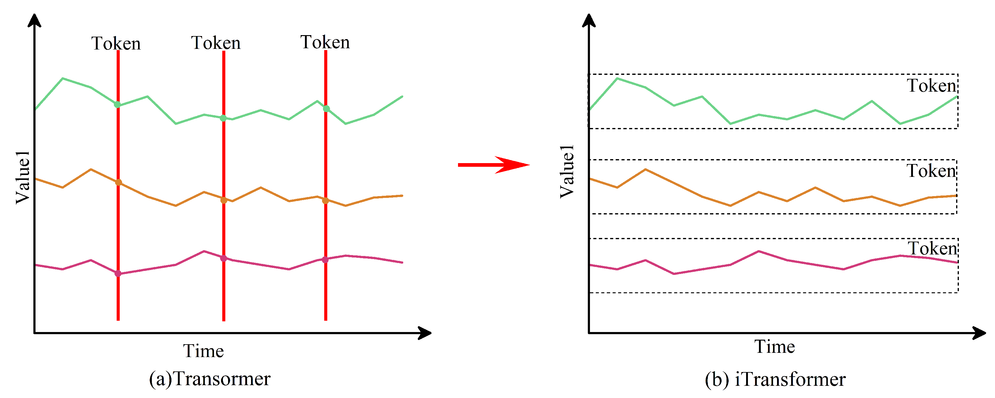
iTransformer is a structurally modified variant of the Transformer specifically designed for time-series forecasting. In standard Transformer models, inputs are tokenized along the temporal axis so that each token contains the feature vector of all variables at a single time step. This time-tokenization has two main limitations. First, because attention operates over time tokens, modeling very long-range temporal dependencies becomes computationally expensive, which restricts the effective receptive field. Second, although variables are contained within the same time token, the strict sequential progression of tokens may weaken the ability to model direct cross-variable dependencies over long horizons [20].
To address these limitations, iTransformer adopts a variable-first tokenization: the input is reoriented so that each token corresponds to the entire temporal trajectory of a single variable over the input window. In other words, tokens are created along the variable dimension; each token stores a variable’s sequence across T time steps. This tokenization preserves the full temporal information of each variable within a token and enables attention to directly model long-range dependencies between variables.
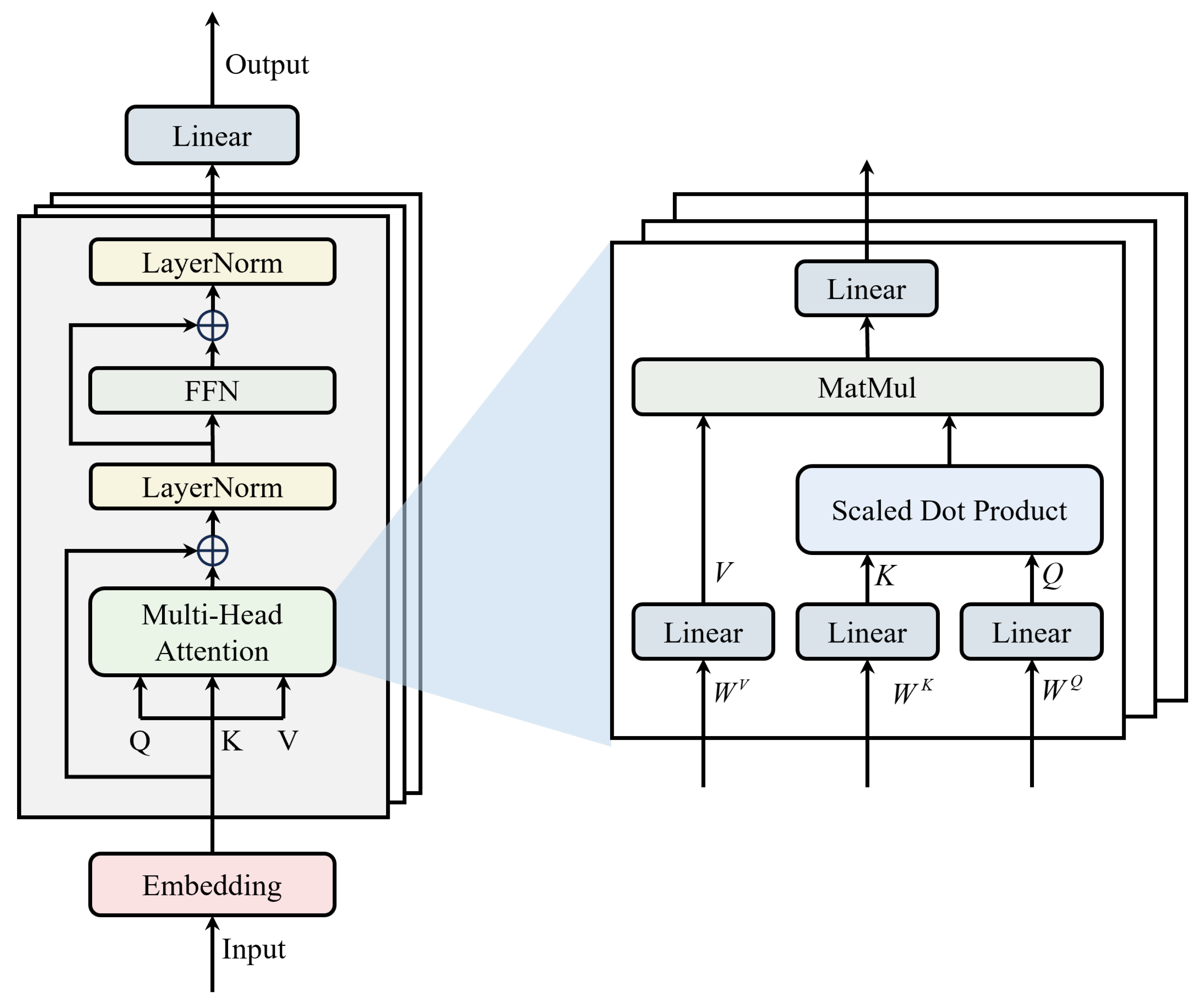
Figure 3 compares the token embedding schemes of the standard Transformer and iTransformer, and Figure 4 presents the overall iTransformer architecture. The model follows the standard Transformer pipeline—an embedding layer, stacked encoder blocks, and an output mapping—but differs in the token construction and embedding step. The input (either a noise sequence z or real/generated sequence x r e a l / x g e n ) is first reoriented (variables ↔ time) and linearly projected into a fixed embedding dimension d m o d e l . The resulting tokens are then processed by stacked encoder layers.
The multi-head attention module captures relationships between tokens by computing the scaled dot-product attention for each head:
Attention ( Q , K , V ) = softmax Q K T d k V ,
and the multi-head output is
MultiHead ( Q , K , V ) = Concat ( head 1 , head 2 , , head h ) W O ,
where h e a d i = A t t e n t i o n ( Q W i Q , K W i K , V W i V ) , and W O is the output projection. A dropout layer is typically applied to the projected multi-head output:
Out M H = Dropout ( MultiHead ( Q , K , V ) ) ,
The encoder uses residual connections and layer normalization. Denoting the input to the attention sublayer as X, the post-attention output with residual connection is
Out LN = LayerNorm ( X + Out MH ) ,
The feedforward sublayer (FFN) applies two linear projections with a nonlinear activation (e.g., ReLU or GELU):
FFN ( x ) = W 2 σ ( W 1 x + b 1 ) + b 2 ,
and its output is
Out FFN = FFN ( Out LN ) ,
The encoder layer output is then obtained by the second residual connection and layer normalization:
Out iT = LayerNorm ( Out LN + Out FFN ) ,
This variable-first tokenization combined with standard Transformer encoder mechanics enables iTransformer to (1) preserve full per-variable temporal patterns within tokens and (2) allow attention to directly capture long-range cross-variable dependencies, while keeping the remainder of the Transformer pipeline familiar and implementable.

3.2.3. Dynamically Gated Feature Fusion

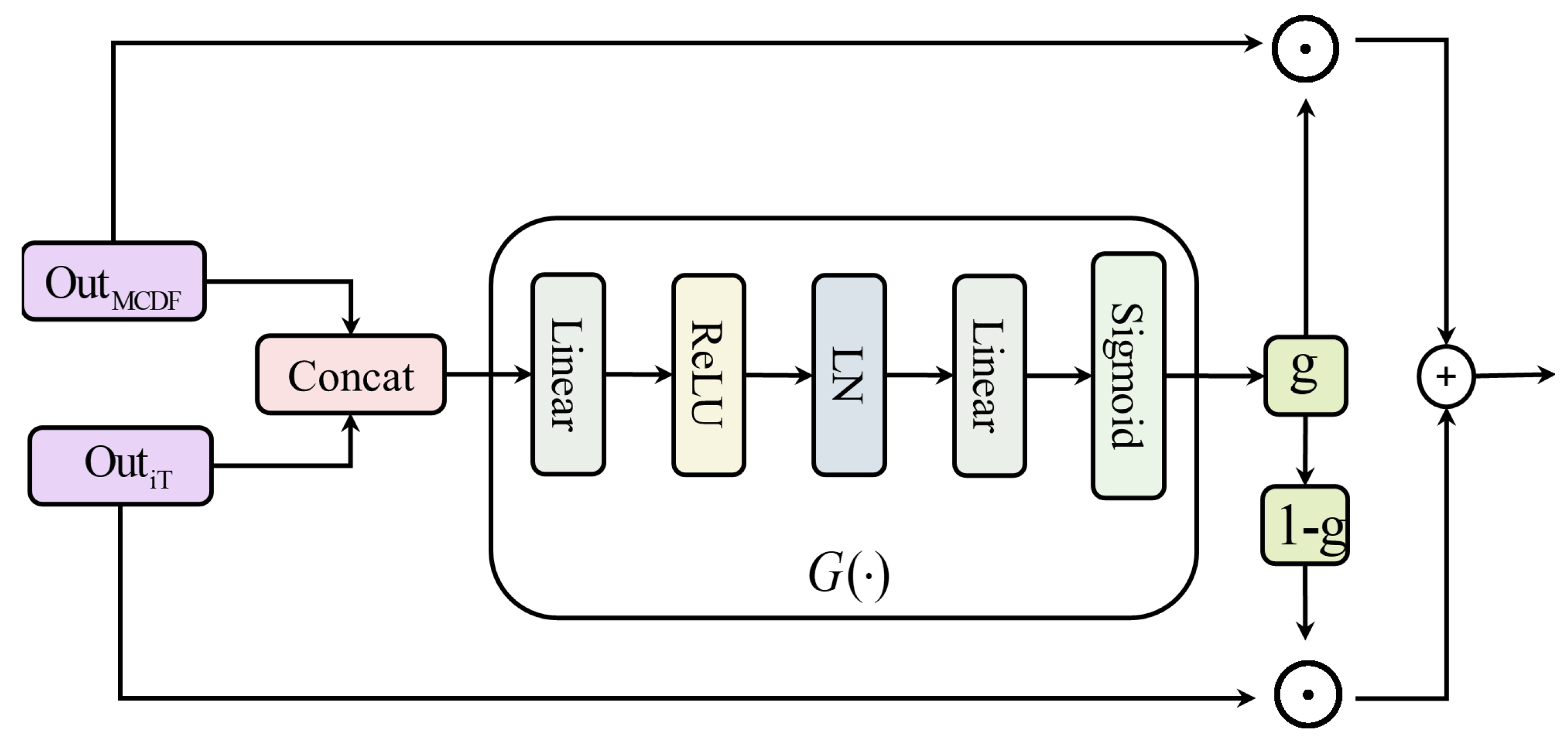
In MiT-WGAN, the dynamic gating fusion (DGF) module adaptively integrates the outputs from two feature-extraction paths—the multi-convolution dynamic fusion (MCDF) branch and the improved Transformer (iTransformer). As illustrated in Figure 5, DGF differs from static fusion schemes (e.g., simple concatenation or fixed-weight averaging). Instead, it employs a gating-vector generation subnetwork that dynamically learns the relative contributions of the two feature types during training in an end-to-end manner.
Specifically, let O u t M C D F , O u t i T R T × d denote the outputs of the MCDF and iTransformer branches, respectively. These are concatenated along the channel (feature) dimension:
F cat = Out MCDF ; Out iT R T × 2 d ,
The concatenated feature vector is fed to the gating subnetwork, which applies a linear layer, a ReLU nonlinearity, and layer normalization (LN) to extract high-level features. Then, a second linear layer projects the representation to the gating dimension, and a final sigmoid activation produces the gating vector g.
g = σ ( LN ( ReLU ( F cat W d 1 + b d 1 ) ) W d 2 + b d 2 ) ,
where W d 1 , W d 2 and b d 1 , b d 2 are learnable weight matrices and biases of the gating network.
During training, the gating vector g and its complement 1 g modulate the two feature branches through element-wise weighting:
Out D G F = g Out M C D F + ( 1 g ) Out i T ,
where ⊙ denotes elementwise (Hadamard) multiplication. The gating vector g performs weighted adjustments on the outputs of MCDF and iTransformer, ensuring that the model can adaptively distribute importance between local convolutional features and global temporal features. O u t D G F is then forwarded to subsequent network layers for further processing.

3.3. Loss Update

The training of a GAN is fundamentally an optimization process based on stochastic gradient descent (SGD). In each iteration, a mini-batch of real logarithmic returns is sampled from the true data distribution P d a t a , while a mini-batch of random noise vectors is drawn from the noise distribution P z . The generator G maps the noise vectors to the generated data space, updates its parameters θ g , and minimizes the generator loss. Simultaneously, the discriminator D attempts to distinguish between real and generated logarithmic returns, updates its parameters θ d , and minimizes the discriminator loss [36].
However, GAN training is notoriously challenging. When employing the conventional value function (Equation (4)), the training process may become unstable due to vanishing or exploding gradients, which hinders the optimization of both the generator and the discriminator.
To address this problem, the Wasserstein Generative Adversarial Network [21] introduces the Wasserstein-1 distance (also called the Earth Mover’s Distance) to replace the traditional loss function, while the gradient-penalized variant WGAN-GP is defined by Gulrajani et al. (2017) [22]. Let the probability distribution of the real data be P r and that of the generated data be P g . The Wasserstein-1 distance is defined as
W ( P r , P g ) = inf γ Π ( P r , P g ) E ( X real , X gen ) γ X real X gen ,
where Π ( P r , P g ) represents the set of all joint distributions, with P r and P g as marginal distributions. According to the Kantorovich–Rubinstein duality, Equation (21) can be rewritten as
W ( P r , P g ) = sup f r 1 E x P r [ f ( x ) ] E x P g [ f ( x ) ] ,
where f r 1 means that f is a 1-Lipschitz function. In WGAN, the discriminator aims to approximate this 1-Lipschitz function, and its loss function is expressed as
L = E x P r [ D ( x ) ] E z P z [ D ( G ( z ) ) ] ,
In order to ensure f r 1 , Gulrajani et al. [22] introduced a gradient penalty (GP) in WGAN. The enhanced loss function is defined as follows:
L WGAN - GP = E x P r [ D ( x ) ] E z P z [ D ( G ( z ) ) ] + λ E x ^ P x ^ x ^ D ( x ^ ) 2 1 2 ,
Among the aforementioned elements, λ is the gradient penalty coefficient. x ^ is the sample obtained by random interpolation between the real data and the generated data, expressed as
x ^ = ϵ · X real + ( 1 ϵ ) · X gen , ϵ U ( 0 , 1 ) ,
The objective of the generator is to produce samples that will achieve higher scores when evaluated by a discriminator D. Consequently, the generator loss can be expressed as a function of the objective function WGAN-GP:
L G = E z p ( z ) [ D ( G ( z ) ) ] ,
During training, the critic and generator are updated in an alternating fashion. The discriminator is typically updated n (≥1) times to better approximate the Wasserstein distance, followed by a single generator update.

3.4. Theoretical Motivation

In the design of MiT-WGAN, the incorporation of WGAN-GP establishes a robust adversarial training framework, effectively mitigating challenges such as vanishing gradients and mode collapse. This facilitates stable model convergence even under the complex distributions characteristic of financial time series. Nevertheless, the improved performance of the model is not solely attributed to stable optimization but also derives from the intrinsic learning biases and complementary strengths of its heterogeneous submodules.
Specifically, the multi-convolutional dynamic fusion (MCDF) module demonstrates a natural aptitude for extracting local patterns, including short-term volatility clustering and burst dynamics, thereby providing clear advantages in addressing high-frequency local fluctuations. In contrast, the iTransformer module emphasizes the modeling of long-range dependencies and global trends, enabling a more comprehensive representation of macro-level dynamics and inter-period correlations intrinsic to financial time series. The dynamic gated fusion (DGF) mechanism further harmonizes these distinct biases by adaptively integrating local and global information through dynamic weight allocation, thereby avoiding the dominance or underrepresentation of any single architectural bias.
Consequently, compared with approaches that rely exclusively on convolutional networks or Transformer architectures, MiT-WGAN achieves a more holistic characterization of the multi-scale structure of financial time series. This balance between local sensitivity and long-term consistency underpins the superior performance of the proposed method relative to existing alternatives.
At the same time, financial time series typically exhibit pronounced nonstationarity and high noise levels, which pose additional challenges for generative modeling. To mitigate nonstationarity, we apply log-return transformation, z-score standardization, and a Lambert-W-based transformation during preprocessing to attenuate trend, skewness, and heavy-tail behavior. At the model level, the complementary strengths of MCDF and iTransformer improve adaptability to structural changes and regime shifts in the market. To address noise, the adversarial training of WGAN-GP encourages the generator to match the underlying data distribution rather than random perturbations, while the DGF module further reconciles local and global information via adaptive gating, thereby reducing the risk of noise dominance.

4. Experiment

All experiments conducted in this study were implemented in Python (version: 3.8.19). The model and training pipeline were built with PyTorch (version: 1.8.0). Training was accelerated using PyTorch’s CUDA backend on an NVIDIA RTX 4060 Ti GPU. For data preprocessing and evaluation, NumPy and pandas were used. In the comparative experiments, all baseline models were evaluated using their official implementations or the configurations specified in the original literature. To ensure fairness and reliability, key hyperparameters were carefully tuned within an appropriate range during the experimental setup.
Concurrently, a detailed enumeration of the hyperparameter settings for each module of the MiT-WGAN model is provided (see Table 1). These include the convolutional kernel sizes and channel numbers of the MCDF convolution branch, the number of layers, attention heads, and hidden dimensions of the iTransformer, as well as the relevant parameters of the dynamic gating fusion module.

4.1. Data Preprocessing

We used real-world stock price data for two S&P 500 constituents to evaluate MiT-WGAN. Specifically, we consider Apple (AAPL) and Amazon (AMZN). For GAN training, only closing prices were used. Raw closing-price series were preprocessed to construct the training set. The preprocessing pipeline is illustrated in Figure 6.
  • Initially, for the AAPL and AMZN datasets, the actual closing prices are retrieved.
  • For the real closing prices of the two datasets, the logarithmic return rate is calculated as follows:
    r t = ln P t P t 1 , t = 1 , 2 , , T ,
    where P t represents the asset price at time t.
  • Subsequently, the calculated logarithmic return data is standardized and converted into a series with zero mean and unit variance.
  • In order to resolve the contradiction between the model’s generative capabilities and the heavy-tailed nature of financial data, the standardized data is further processed using the Lambert W transformation [27].
  • Subsequently, a secondary normalization is required to further scale the data to the interval [−1, 1].
  • In order to facilitate the model’s capacity to discern the potential representation between data points, a sliding window approach is employed. The dimensions of the sliding window are set to 128, and the step size is designated as 1.

4.2. Experimental Results

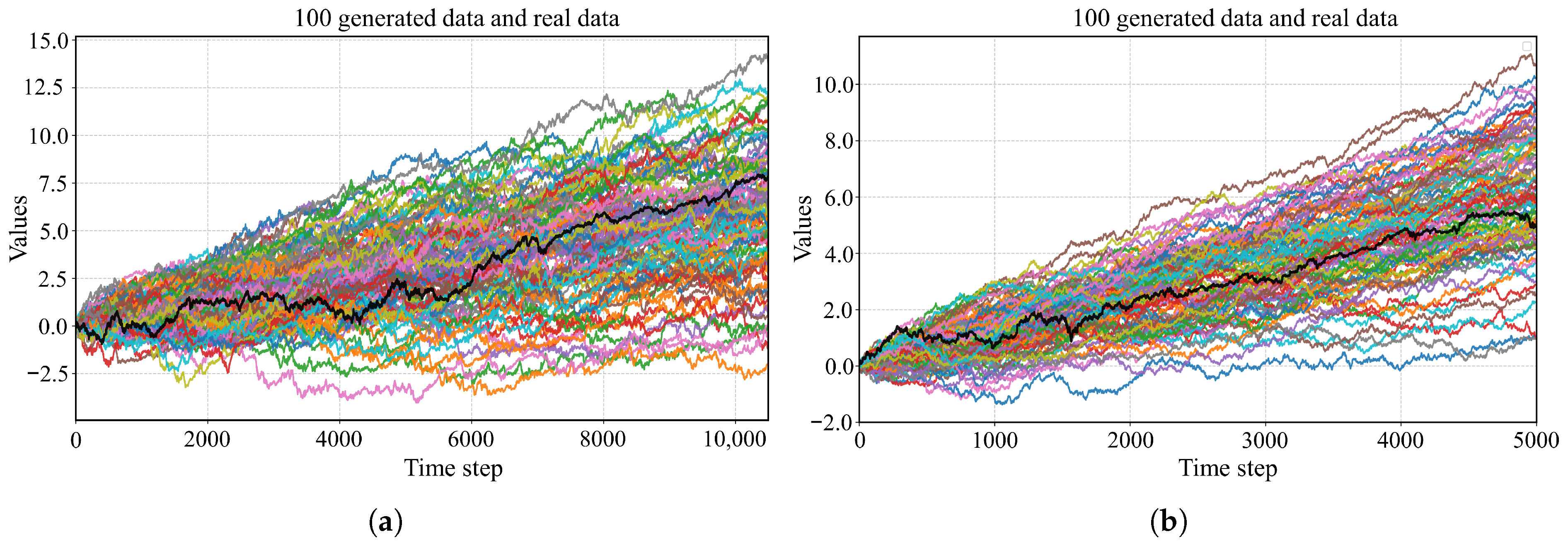
This study used the same experimental setup to train on the AAPL and AMZN datasets. The trained model was then used to generate 100 trajectories of logarithmic returns, and price paths were reconstructed from these returns and backtested against the realized prices.
Figure 7 compares the realized prices (black curve) with the price paths reconstructed from the generated log-returns. As expected, the generated series closely track the realized series in overall trends and volatility. Across the 100 generated trajectories, the mean-reversion tendency of the MiT-WGAN-generated series largely coincides with the realized series, demonstrating the model’s ability to capture key statistical characteristics of financial time series. In addition, the generated samples exhibit volatility clustering and asymmetry, consistent with stylized facts in financial markets. This suggests that the model not only matches marginal distributions but also reproduces typical structural characteristics of financial time series.
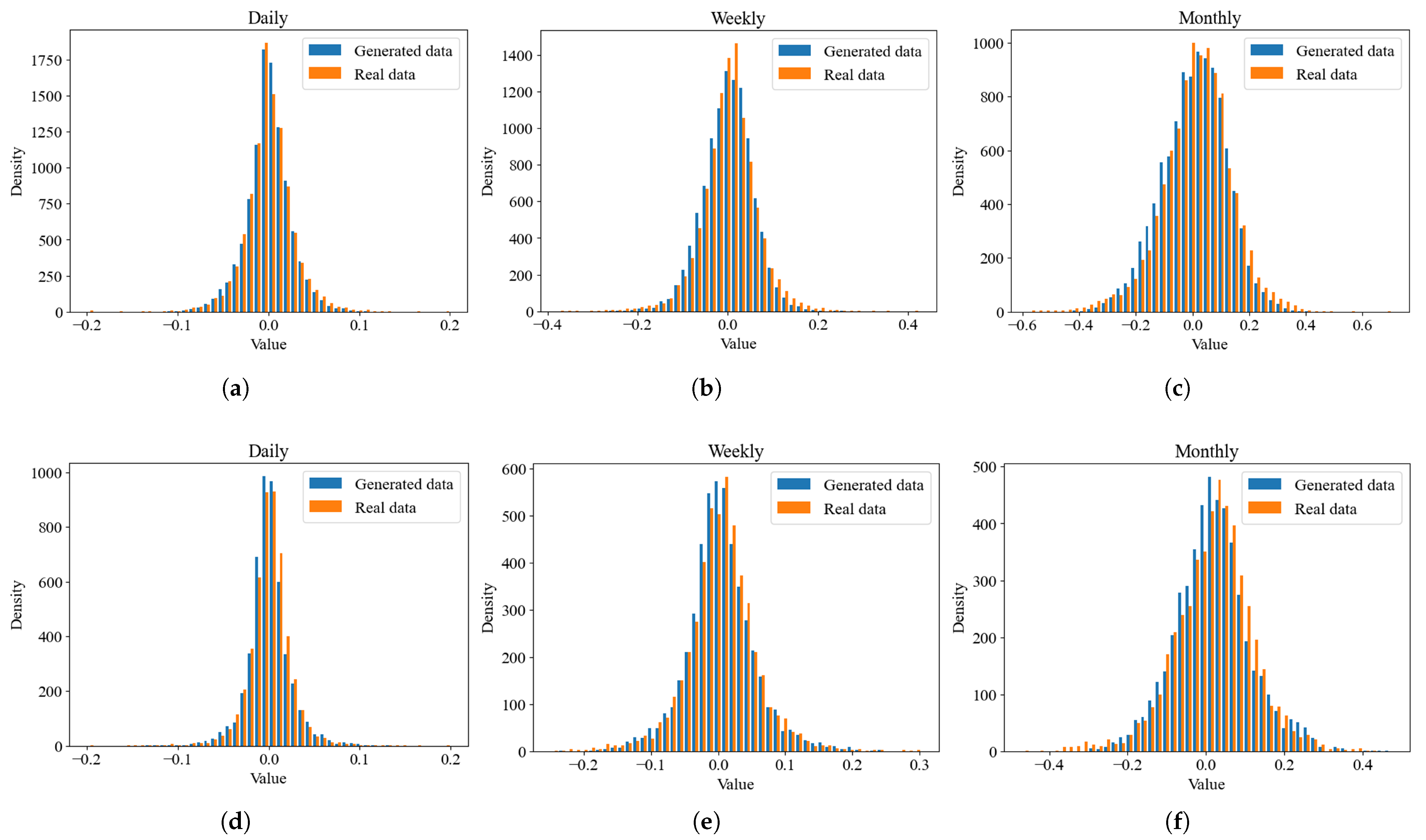
To further assess the distributional fidelity of the proposed MiT-WGAN, we plotted comparative density curves between realized prices and prices reconstructed from the generated returns at three time scales (daily, weekly, and monthly), as shown in Figure 8. The distributions of the generated price series closely resemble those of the real data across all three time scales, particularly in central tendency and overall symmetry. These results indicate that the model not only matches first-order statistics (mean and variance) but also aligns with higher-order moments (skewness and kurtosis).
At the daily scale, the generated samples are tightly concentrated around a zero mean and closely match the realized data in the tails, demonstrating the model’s ability to capture the heavy-tailed nature of returns. At the weekly and monthly scales, as temporal aggregation increases, the empirical distribution gradually approaches normality, and the MiT-WGAN-generated series also reproduces this trend. These observations indicate that the model not only fits market data at a single time scale but also preserves key statistical patterns across multiple scales.
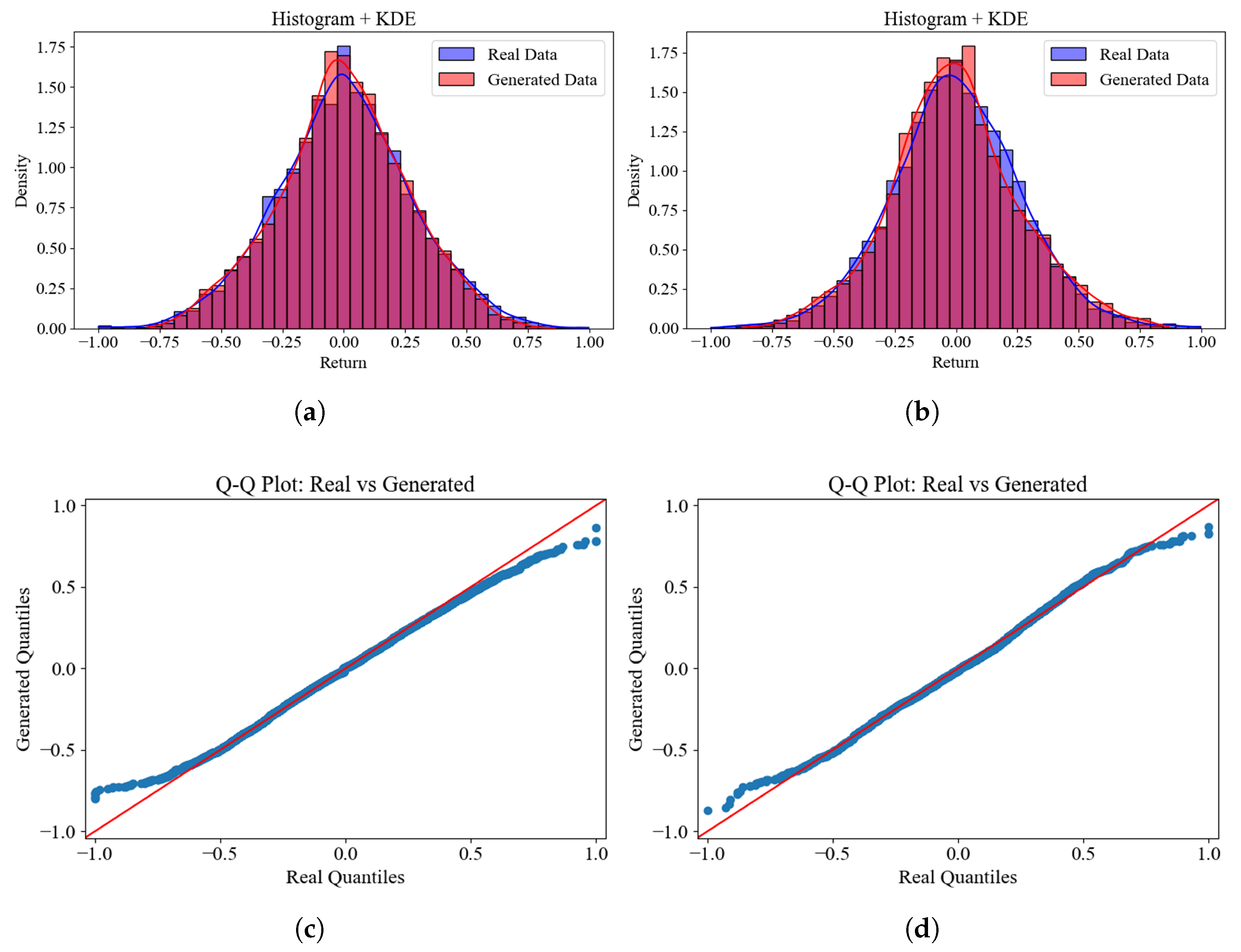
Figure 9 compares histograms, kernel density estimates (KDEs), and Q–Q plots for the generated and realized log-returns. Inspection of the histograms and KDEs shows close agreement in distributional shape between the generated and realized series. Both exhibit a pronounced central peak and heavy tails (leptokurtosis). At the center, the modal peaks essentially coincide, indicating that MiT-WGAN effectively captures the central tendency of the return distribution. Furthermore, the Q–Q plots place the generated and realized quantiles close to the 45° reference line, indicating high overall distributional consistency. Across the AAPL and AMZN datasets, these results demonstrate that MiT-WGAN reproduces key distributional characteristics of market returns.
In addition, we conducted experimental comparisons to assess the generative performance of the proposed method against state-of-the-art baselines. Specifically, we compared MiT-WGAN with three baselines—QuantGAN, TimeGAN, and a GARCH benchmark. To enable a fair comparison across the four models, we employed a common set of evaluation metrics.
  • The Earth Mover’s Distance (EMD, also known as the Wasserstein-1 distance): This metric quantifies the discrepancy between the distributions of real and generated sequences. The Wasserstein-1 distance is formally defined as
    W 1 ( P r , P g ) = inf γ Π ( P r , P g ) E ( x , y ) γ [ | x y | ] ,
    where Π ( P r , P g ) denotes the set of all joint distributions with marginals P r and P g . In practice, we approximate the EMD using empirical samples of real logarithmic returns x r e a l and generated returns x g e n . By aligning the sorted samples, the discrete approximation is given by
    EMD ( X , Y ) = 1 n i = 1 n x ( i ) real x ( i ) gen ,
    where x ( i ) real and x ( i ) gen denote the i-th ordered statistics (sorted samples). This formulation corresponds to the empirical approximation of the Wasserstein-1 distance and ensures robustness in capturing the distributional discrepancy.
  • ACF-Score: A key property of financial log-return series is that their linear autocorrelations are typically close to zero, whereas the autocorrelations of their absolute and squared values are significant, reflecting volatility clustering. Accordingly, we compute the autocorrelation functions of the raw log-return r t , the absolute log-return | r t | , and the squared return r t 2 and compare them between the real and generated series. Given a lag order k (set to 10 in this study), the autocorrelation is defined as
    ρ ( k ) = Cov ( r t , r t + k ) Var ( r t ) Var ( r t + k ) ,
    The discrepancy between the autocorrelation functions (ACFs) of the real log-return series and the generated log-return series is quantified using the mean squared error (MSE):
    ACF - Score = 1 K k = 1 K ρ real ( k ) ρ gen ( k ) 2 ,
  • Leverage Effect Score: The negative correlation between returns and future volatility is a well-documented nonlinear feature of financial time series, known as the leverage effect. It is computed as the correlation between the log-return and its future squared log-return, expressed as
    Lev = ρ ( r t , r t + 1 2 ) real ρ ( r t , r t + 1 2 ) gen ,
    A smaller value of this metric indicates that the generated data more accurately reproduces the leverage effect observed in real markets.
  • Maximum Mean Discrepancy (MMD): To further evaluate the distribution similarity between the real sequence and the generated sequence, the Maximum Mean Discrepancy was calculated. The two groups of samples are denoted by X = { x i } i = 1 n and Y = { y j } j = 1 m , respectively, and the square form is defined as follows:
    MMD 2 ( X , Y ) = 1 n 2 i , i k ( x i , x i ) + 1 m 2 j , j k ( y j , y j ) 2 n m i , j k ( x i , y j ) ,
    where k ( · , · ) represents the Gaussian kernel function. The smaller the MMD value is, the closer the distribution of the generated data is to the real data distribution.
Table 2 reports the evaluation scores of MiT-WGAN and three baseline methods across two stock datasets. For both AAPL and AMZN, MiT-WGAN outperforms the baselines across multiple evaluation metrics. In terms of the EMD metric, which measures overall distributional discrepancy, MiT-WGAN achieves the lowest score—substantially lower than TimeGAN and GARCH and slightly lower than QuantGAN. This indicates that the marginal distribution of MiT-WGAN-generated data aligns more closely with the realized data.
In terms of autocorrelation metrics, MiT-WGAN attains lower scores on the raw series autocorrelation (ACF( r t )), the absolute-return autocorrelation (ACF( | r t | )), and the squared-return autocorrelation (ACF( r t 2 )). This demonstrates that, relative to the other three models, MiT-WGAN more effectively captures the weakly stationary properties of return series. On the AMZN dataset, MiT-WGAN shows superior performance in both ACF( | r t | ) and ACF( r t 2 ), confirming its stronger ability to characterize volatility clustering and nonlinear dependence.
Furthermore, MiT-WGAN demonstrates a pronounced advantage in the Leverage Effect metric, achieving markedly lower values than QuantGAN, TimeGAN, and GARCH. This result suggests that MiT-WGAN possesses a superior ability to capture the asymmetric impact of negative returns on future volatility in financial markets. In addition, MiT-WGAN consistently attained the lowest MMD values across both datasets, highlighting a notable improvement over existing methods. Collectively, these findings reinforce the conclusion that MiT-WGAN achieves a higher degree of accuracy in overall distribution fitting.

4.3. Tail Risk Evaluation

To further evaluate the ability of MiT-WGAN to capture extreme events, we employed tail risk metrics widely adopted in financial risk management, namely, value-at-risk (VaR) and conditional value-at-risk (CVaR, also referred to as Expected Shortfall). These metrics were assessed at the 95% and 99% confidence levels.
Formally, for a return sequence r t , the VaR at confidence level α is defined as the ( 1 α ) quantile of the distribution.
VaR α ( r ) = inf { q R : P ( r t q ) 1 α } ,
CVaR is defined as the conditional expected loss of the portion exceeding the VaR threshold.
CVaR α ( r ) = E [ r t r t VaR α ( r ) ] ,
In Table 3, we present a comparative analysis of the VaR and CVaR results for MiT-WGAN and three baseline models on the AAPL and AMZN datasets at the 95% and 99% confidence levels. The degree to which the VaR and CVaR of the generated data approximate the empirical values reflects the model’s ability to accurately capture the distribution of extreme events.
As shown in Table 3, when applied to both datasets, all models in this study generally exhibit a tendency to overestimate risk, as reflected in the more negative VaR and CVaR values compared with those of the empirical data. This pattern suggests a systematic bias toward overestimation in the tail distribution. In most cases, however, the VaR and CVaR values produced by MiT-WGAN are more closely aligned with the empirical benchmarks, thereby demonstrating superior tail-fitting accuracy relative to QuantGAN, GARCH, and TimeGAN. For instance, on the AAPL dataset at the 95% confidence level, the empirical VaR is −0.191. MiT-WGAN yields −0.357, which represents a smaller deviation than those of QuantGAN (−0.424) and TimeGAN (−0.634). This result underscores the effectiveness of MiT-WGAN in capturing the tail distribution and highlights its superiority over QuantGAN and TimeGAN in this regard. A comparable advantage is also observed for the AMZN dataset, where MiT-WGAN achieves smaller deviations in both VaR and CVaR, thereby confirming the model’s robustness across different asset classes.
To further evaluate the robustness of MiT-WGAN under high-volatility conditions, we extracted a high-volatility subset corresponding to the top 10% of the 21-day rolling volatility from both the real and generated series of AAPL and AMZN. VaR and CVaR were then computed on this subset, and the results are reported in Table 4.
A comparison of the empirical VaR and CVaR values in the high-volatility subset with those of the full sample reveals that they are substantially more negative, thereby confirming the amplification of tail risk during turbulent periods. In this context, the VaR and CVaR of the MiT-WGAN-generated data also become more negative, reflecting a certain degree of risk overestimation. Nevertheless, for AAPL, the deviation in the high-volatility subset is narrower than that observed in the full sample, indicating that the model’s tail fitting is closer to reality under high-volatility conditions. By contrast, the results for AMZN exhibit only marginal improvements in the bias of certain indicators, suggesting that the model’s performance may vary across different underlying assets.

4.4. Ablation Study

To validate the effectiveness of the key modules in the proposed model, three sets of ablation experiments were conducted. These experiments involved targeted modifications to the generator and discriminator architectures, which were evaluated under identical training configurations. The ablation design primarily focused on the MCDF, iTransformer, and DGF modules.
  • Removal of the MCDF module: To assess the contribution of the convolutional branch in capturing local dependencies and volatility clustering, the MCDF module was removed, leaving only the iTransformer branch to directly generate logarithmic return series. Under this configuration, the model relies primarily on the iTransformer’s ability to capture long-range dependencies, thereby highlighting the essential role of local convolutional features in modeling short-term volatility patterns.
  • Removal of the iTransformer module: Conversely, to examine the importance of global time-series modeling, the iTransformer branch was removed, retaining only the multi-convolutional dynamic fusion (MCDF) module. In this setting, the generated data depends solely on the convolutional architecture for feature extraction, which has been shown to be effective in capturing short-term dependency patterns. However, this approach is insufficient for adequately modeling long-term dependencies and the overall temporal structure. This experiment thereby facilitates an evaluation of the iTransformer’s effectiveness in capturing long-term dependencies in financial time series.
  • Removal of the DGF module: To evaluate the role of the dynamic gated fusion (DGF) module in information interaction and feature integration, a simple linear fusion strategy was adopted. In this setting, the outputs of the MCDF and iTransformer branches were combined through direct weighted summation or concatenation before mapping, without incorporating a gating mechanism. Comparing this simplified variant with the full model enables a clear assessment of the gating mechanism’s contribution to enhancing feature interaction and overall generation quality.
As shown in Table 5, the ablation results on the AAPL and AMZN datasets are reported. The full MiT-WGAN consistently achieves optimal or near-optimal performance across all evaluation metrics. In contrast, the removal of any single module leads to a substantial degradation in performance, thereby underscoring the critical role of each component within the overall framework.
Specifically, removing the MCDF module resulted in a substantial degradation in the EMD and ACF( ( · ) 2 ) metrics, underscoring the critical role of multi-convolutional dynamic fusion in capturing local dependencies and volatility clustering. The most pronounced decline was observed when the iTransformer module was removed, particularly in the ACF(id) and Leverage Effect metrics. This result highlights the iTransformer’s pivotal role in modeling long-range dependencies and asymmetric effects. Similarly, removing the DGF module also led to a marked reduction in performance, especially in MMD2 and Leverage Effect, indicating that the absence of dynamic gating weakens the integration of local features with global dependencies.

5. Discussion and Future Work

This study introduces a generative adversarial network (MiT-WGAN) for synthesizing financial log-returns. To enhance generation quality and stabilize training, MiT-WGAN embeds a multi-convolutional fusion module in parallel with the iTransformer, integrates a dynamic gated fusion unit, and incorporates the WGAN-GP framework. These architectural enhancements collectively strengthen the model’s capacity to generate realistic log-returns. Experimental validation on two S&P 500 stocks, supported by extensive visual analyses and comparisons with multiple generative models, confirms the effectiveness of MiT-WGAN in financial time-series generation, where it significantly outperforms baseline models.
Despite MiT-WGAN’s notable gains in sample quality and in preserving salient properties of financial time series, its ability to reproduce extreme tails remains limited. As shown in Figure 9 (e.g., the tail displacement in the Q–Q plot), the model underrepresents the distribution of rare, high-volatility episodes and shock events. This shortcoming can bias applications that depend on tail behavior, such as risk measurement and stress-testing. Although the model captures the monotonic increase in tail risk as the confidence level rises, it systematically overestimates the magnitude: the VaR and CVaR of the generated series are more negative than the empirical benchmarks, with the bias amplified at the 99% level. These results indicate that MiT-WGAN does not yet adequately model the far tails and fails to accurately reflect the size of losses observed during turbulent market conditions.
Future work will focus on improving the model’s capacity to account for extreme values. One promising direction is to incorporate conditional information—such as macroeconomic variables, market sentiment indicators, or policy event signals—into the generative process to better capture the conditional dependencies underlying extreme events. Such integration would not only improve accuracy in modeling tail distributions but also increase the practical relevance of generated sequences for risk management and quantitative investment. Additionally, introducing constraint mechanisms grounded in financial theory or designing hybrid loss functions represents another important avenue for future research.

Author Contributions

Conceptualization, L.Z. and C.L.; methodology, C.L.; software, C.L.; validation, C.L.; formal analysis, C.L.; investigation, C.L.; resources, L.Z.; data curation, C.L.; writing—original draft preparation, L.Z. and C.L.; writing—review and editing, L.Z.; visualization, C.L.; supervision, L.Z.; project administration, L.Z.; funding acquisition, L.Z. All authors have read and agreed to the published version of the manuscript.

Funding

This research was funded by Research on Online Deep Transfer Learning of Time Series based on Financial Data (Grant No: Qian Ke He Ji Chu [2024] general 520) supported by Guizhou Province Basic Research Plan (Natural Sciences) Projects. Additionally, it received funding from the Sixth Batch of Gui-Zhou Province High-level Innovative Talent Training Program (Grant No.: Zhu Ke He Tong [2022]011) and the Guiyang University New Degree Awarding Point Cultivation and Construction Project in 2025 [Gyxk202502].

Data Availability Statement

The data will be available on reasonable request.

Acknowledgments

The authors would like to express their sincere gratitude to the School of Electronic Information Engineering of Guiyang University for providing a favorable research environment for promoting the integration of FinTech and deep learning methods. In addition, they would like to express their sincerest gratitude to every researcher who provided assistance in this research.

Conflicts of Interest

The authors declare no conflicts of interest.

References

  1. Lim, B.; Zohren, S. Time-series forecasting with deep learning: A survey. Philos. Trans. R. Soc. A 2021, 379, 20200209. [Google Scholar] [CrossRef]
  2. Kumar, N.; Susan, S. COVID-19 pandemic prediction using time series forecasting models. In Proceedings of the 2020 11th International Conference on Computing, Communication and Networking Technologies (ICCCNT), Kharagpur, India, 1–3 July 2020; IEEE: Piscataway, NJ, USA, 2020; pp. 1–7. [Google Scholar]
  3. Sousa, M.R.; Gama, J.; Brandão, E. A new dynamic modeling framework for credit risk assessment. Expert Syst. Appl. 2016, 45, 341–351. [Google Scholar] [CrossRef]
  4. Fabozzi, F.A.; Simonian, J.; Fabozzi, F.J. Risk parity: The democratization of risk in asset allocation. J. Portf. Manag. 2021, 47, 41–50. [Google Scholar] [CrossRef]
  5. Acharya, V.V. A theory of systemic risk and design of prudential bank regulation. J. Financ. Stab. 2009, 5, 224–255. [Google Scholar] [CrossRef]
  6. Goodell, J.W.; Goutte, S. Co-movement of COVID-19 and Bitcoin: Evidence from wavelet coherence analysis. Financ. Res. Lett. 2021, 38, 101625. [Google Scholar] [CrossRef] [PubMed]
  7. McRandal, R.; Rozanov, A. A primer on tail risk hedging. J. Secur. Oper. Custody 2012, 5, 29–36. [Google Scholar] [CrossRef]
  8. Yoon, J.; Jarrett, D.; Van der Schaar, M. Time-series generative adversarial networks. Adv. Neural Inf. Process. Syst. 2019, 32, 5508–5518. [Google Scholar]
  9. Smith, K.E.; Smith, A.O. Conditional GAN for timeseries generation. arXiv 2020, arXiv:2006.16477. [Google Scholar] [CrossRef]
  10. Goodfellow, I.J.; Pouget-Abadie, J.; Mirza, M.; Xu, B.; Warde-Farley, D.; Ozair, S.; Courville, A.; Bengio, Y. Generative adversarial nets. Adv. Neural Inf. Process. Syst. 2014, 27, 2672–2680. [Google Scholar]
  11. Wang, M.; El-Gayar, O. Generative adversarial networks in fraud detection: A systematic literature review. In Proceedings of the Americas Conference on Information Systems (AMCIS), Salt Lake City, UT, USA, 15–17 August 2024; Available online: https://aisel.aisnet.org/amcis2024/security/security/35/ (accessed on 1 October 2025).
  12. Yang, X.; Li, C.; Han, Z.; Lu, Z. Distributed Generative Adversarial Networks for Fuzzy Portfolio Optimization. In Proceedings of the International Conference on Algorithms and Architectures for Parallel Processing, Tianjin, China, 20–22 October 2023; Springer Nature: Singapore, 2023; pp. 236–247. [Google Scholar]
  13. Zhou, X.; Pan, Z.; Hu, G.; Tang, S.; Zhao, C. Stock market prediction on high-frequency data using generative adversarial nets. Math. Probl. Eng. 2018, 2018, 4907423. [Google Scholar] [CrossRef]
  14. Esteban, C.; Hyland, S.L.; Rätsch, G. Real-valued (medical) time series generation with recurrent conditional GANs. arXiv 2017, arXiv:1706.02633. [Google Scholar] [CrossRef]
  15. Borovykh, A.; Bohte, S.; Oosterlee, C.W. Conditional time series forecasting with convolutional neural networks. arXiv 2017, arXiv:1703.04691. [Google Scholar]
  16. Bai, S.; Kolter, J.Z.; Koltun, V. An empirical evaluation of generic convolutional and recurrent networks for sequence modeling. arXiv 2018, arXiv:1803.01271. [Google Scholar] [CrossRef]
  17. Zerveas, G.; Jayaraman, S.; Patel, D.; Bhamidipaty, A.; Eickhoff, C. A transformer-based framework for multivariate time series representation learning. In Proceedings of the 27th ACM SIGKDD Conference on Knowledge Discovery & Data Mining, Virtual Event, 14–18 August 2021; pp. 2114–2124. [Google Scholar]
  18. Wen, Q.; Zhou, T.; Zhang, C.; Chen, W.; Ma, Z.; Yan, J.; Sun, L. Transformers in time series: A survey. arXiv 2022, arXiv:2202.07125. [Google Scholar]
  19. Dai, Z.; Liu, H.; Le, Q.V.; Tan, M. CoatNet: Marrying convolution and attention for all data sizes. Adv. Neural Inf. Process. Syst. 2021, 34, 3965–3977. [Google Scholar]
  20. Liu, Y.; Hu, T.; Zhang, H.; Wu, H.; Wang, S.; Ma, L.; Long, M. iTransformer: Inverted transformers are effective for time series forecasting. arXiv 2023, arXiv:2310.06625. [Google Scholar]
  21. Arjovsky, M.; Chintala, S.; Bottou, L. Wasserstein generative adversarial networks. In Proceedings of the International Conference on Machine Learning, Sydney, Australia, 6–11 August 2017; pp. 214–223. [Google Scholar]
  22. Gulrajani, I.; Ahmed, F.; Arjovsky, M.; Dumoulin, V.; Courville, A.C. Improved training of Wasserstein GANs. Adv. Neural Inf. Process. Syst. 2017, 30, 5767–5777. [Google Scholar]
  23. Mogren, O. C-RNN-GAN: Continuous recurrent neural networks with adversarial training. arXiv 2016, arXiv:1611.09904. [Google Scholar]
  24. Yu, L.; Zhang, W.; Wang, J.; Yu, Y. SeqGAN: Sequence generative adversarial nets with policy gradient. In Proceedings of the AAAI Conference on Artificial Intelligence, San Francisco, CA, USA, 4–9 February 2017; Volume 31. [Google Scholar]
  25. Mirza, M.; Osindero, S. Conditional generative adversarial nets. arXiv 2014, arXiv:1411.1784. [Google Scholar] [CrossRef]
  26. Xu, T.K.; Wenliang, L.K.; Munn, M.; Acciaio, B. Cot-GAN: Generating sequential data via causal optimal transport. Adv. Neural Inf. Process. Syst. 2020, 33, 8798–8809. [Google Scholar]
  27. Wiese, M.; Knobloch, R.; Korn, R.; Kretschmer, P. Quant GANs: Deep generation of financial time series. Quant. Financ. 2020, 20, 1419–1440. [Google Scholar] [CrossRef]
  28. Takahashi, S.; Chen, Y.; Tanaka-Ishii, K. Modeling financial time—Series with generative adversarial networks. Phys. A Stat. Mech. Its Appl. 2019, 527, 121261. [Google Scholar] [CrossRef]
  29. Huang, A.; Khushi, M.; Suleiman, B. Regime—Specific Quant Generative Adversarial Network: A Conditional Generative Adversarial Network for Regime—Specific Deepfakes of Financial Time Series. Appl. Sci. 2023, 13, 10639. [Google Scholar] [CrossRef]
  30. Jeon, S.; Seo, J.T. A synthetic time—series generation using a variational recurrent autoencoder with an attention mechanism in an industrial control system. Sensors 2023, 24, 128. [Google Scholar] [CrossRef]
  31. Leushuis, R.M. Probabilistic forecasting with VAR—VAE: Advancing time series forecasting under uncertainty. Inf. Sci. 2025, 713, 122184. [Google Scholar] [CrossRef]
  32. Rasul, K.; Seward, C.; Schuster, I.; Vollgraf, R. Autoregressive denoising diffusion models for multivariate probabilistic time series forecasting. In Proceedings of the International Conference on Machine Learning, PMLR, Virtual, 18–24 July 2021; pp. 8857–8868. [Google Scholar]
  33. Kollovieh, M.; Ansari, A.F.; Bohlke-Schneider, M.; Zschiegner, J.; Wang, H.; Wang, Y.B. Predict, refine, synthesize: Self-guiding diffusion models for probabilistic time series forecasting. Adv. Neural Inf. Process. Syst. 2023, 36, 28341–28364. [Google Scholar]
  34. Meijer, C.; Chen, L.Y. The rise of diffusion models in time—Series forecasting. arXiv 2024, arXiv:2401.03006. [Google Scholar]
  35. Hu, J.; Shen, L.; Sun, G. Squeeze—and—excitation networks. In Proceedings of the IEEE Conference on Computer Vision and Pattern Recognition, Salt Lake City, UT, USA, 18–23 June 2018; IEEE: Piscataway, NJ, USA, 2018; pp. 7132–7141. [Google Scholar]
  36. Pardo, F.D.M.; López, R.C. Mitigating overfitting on financial datasets with generative adversarial networks. J. Financ. Data Sci. 2020, 2, 76–85. [Google Scholar] [CrossRef]
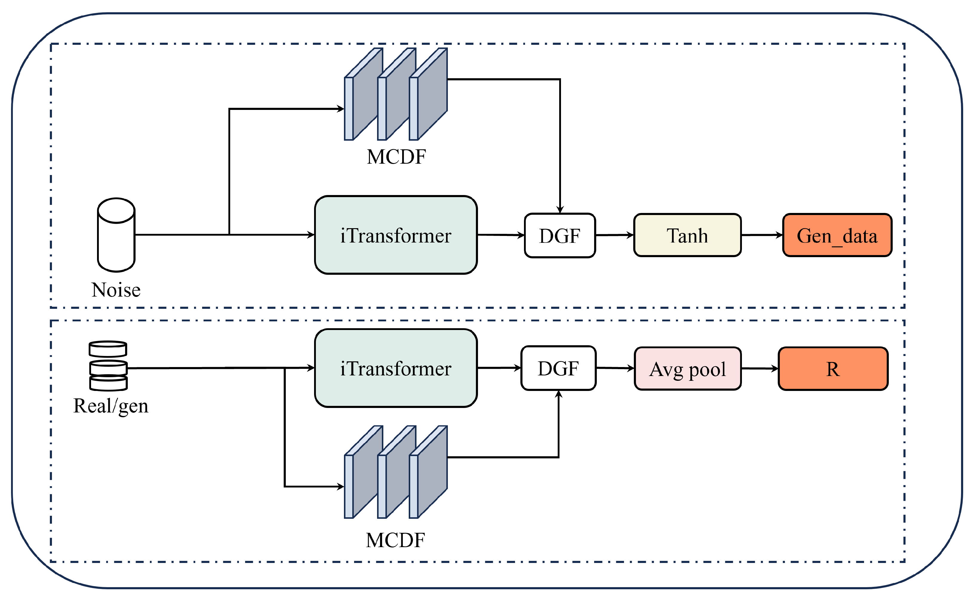
Figure 1. Overview of the MiT-WGAN architecture.
Symmetry 17 01740 g001
Figure 2. Schematic diagram of the multi-convolutional fusion module.
Symmetry 17 01740 g002
Figure 3. Comparison of the token embedding mechanisms in the standard Transformer and the iTransformer.
Symmetry 17 01740 g003
Figure 4. Overview of the iTransformer architecture.
Symmetry 17 01740 g004
Figure 5. Overview of the dynamic gated fusion (DGF) module.
Symmetry 17 01740 g005
Figure 6. Schematic of the data preprocessing procedure.
Symmetry 17 01740 g006
Figure 7. A comparison between MiT-WGAN-generated prices and actual transaction prices for two stock datasets is presented. (a) Real prices and 100 generated trajectories for AAPL; (b) real prices and 100 generated trajectories for AMZN.
Symmetry 17 01740 g007
Figure 8. A comparison between the true and MiT-WGAN-generated densities is presented for two stock datasets. Panels (ac) show the results for the AAPL dataset, and panels (df) show the results for the AMZN dataset.
Symmetry 17 01740 g008
Figure 9. A comparative analysis was performed using histograms, kernel density estimates (KDE), and Q–Q plots of the true and generated log-returns across two stock datasets. The results for the AAPL dataset are presented in panels (a,c), whereas those for the AMZN dataset are shown in panels (b,d).
Symmetry 17 01740 g009
Table 1. Model modules and training hyperparameter settings.
ModuleHyperparametersValue/Setting
MCDFKernel sizes{3, 5, 7}
Channels per conv64
Number of conv3
iTransformerEncoder layers6
Hidden size256
Attention heads8
Dropout rate0.1
Feedforward hidden size1024
NormalizationPre-LayerNorm
Attention typeScaled dot-product
ActivationGELU
DGFFusion typeLearnable gating with sigmoid
Dropout rate0.1
DiscriminatorStructureSymmetric to Generator
NormalizationLayerNorm
TrainingBatch size64
OptimizerAdam ( β 1 = 0 , β 2 = 0.999 )
Learning rate G _ l r = 1 × 10 4 , D _ l r = 5 × 10 5
Epochs200
Table 2. The table reports the evaluation metric scores of the four models, with the best values highlighted in bold.
DatasetMetricsMiT-WGANQuantGANGARCHTimeGAN
AAPLEMD 1.02 × 10 2 1.09 × 10 2 1.28 × 10 2 1.76 × 10 2
ACF(id) 1.51 × 10 4 1.69 × 10 4 1.93 × 10 4 2.56 × 10 4
ACF( | · | ) 1.69 × 10 2 1.85 × 10 2 2.03 × 10 2 2.83 × 10 2
ACF( ( · ) 2 ) 1.49 × 10 2 1.68 × 10 2 1.87 × 10 2 2.70 × 10 2
Leverage Effect 2.15 × 10 2 2.63 × 10 2 3.49 × 10 2 4.32 × 10 2
MMD2 1.51 × 10 2 2.38 × 10 2 3.96 × 10 2 4.64 × 10 2
( ± 2.96 × 10 3 ) ( ± 3.14 × 10 3 ) ( ± 5.90 × 10 3 ) ( ± 4.84 × 10 3 )
AMZNEMD 1.13 × 10 2 1.32 × 10 2 2.25 × 10 2 2.61 × 10 2
ACF(id) 2.41 × 10 4 2.78 × 10 4 3.16 × 10 4 3.97 × 10 4
ACF( | · | ) 2.50 × 10 2 2.92 × 10 2 3.45 × 10 2 4.68 × 10 2
ACF( ( · ) 2 ) 2.35 × 10 2 2.74 × 10 2 3.26 × 10 2 4.38 × 10 2
Leverage Effect 2.28 × 10 2 2.40 × 10 2 2.83 × 10 2 3.52 × 10 2
MMD2 2.41 × 10 2 2.64 × 10 2 3.52 × 10 2 4.96 × 10 2
( ± 1.43 × 10 3 ) ( ± 1.62 × 10 3 ) ( ± 3.06 × 10 3 ) ( ± 4.48 × 10 3 )
Table 3. A comparison of the value-at-risk (VaR) and conditional value-at-risk (CVaR) of the MiT-WGAN with those of the three other baseline models was conducted on generated and real data at 95% and 99% confidence levels (AAPL and AMZN datasets).
DatasetConfidence LevelMetricReal DataMiT-WGANQuantGANGARCHTimeGAN
AAPL95%VaR−0.191−0.357−0.424−0.553−0.634
95%CVaR−0.453−0.678−0.712−0.824−0.948
99%VaR−0.575−0.782−0.873−0.996−1.094
99%CVaR−0.722−0.938−0.994−1.122−1.195
AMZN95%VaR−0.328−0.571−0.647−0.791−0.815
95%CVaR−0.478−0.684−0.722−0.846−0.943
99%VaR−0.501−0.727−0.816−0.916−0.964
99%CVaR−0.641−0.885−0.942−1.171−1.159
Table 4. VaR and CVaR results on the high-volatility subset (top 10% days with highest realized volatility).
MetricAAPL RealAAPL GenAMZN RealAMZN Gen
95% VaR−0.452−0.616−0.591−0.702
95% CVaR−0.568−0.825−0.711−0.815
99% VaR−0.693−0.863−0.783−0.764
99% CVaR−0.743−0.927−0.964−0.905
Table 5. Ablation study results on AAPL and AMZN datasets. The best results are highlighted in bold.
DatasetMetricsFull (MiT-WGAN)w/o MCDFw/o iTransformerw/o DGF
AAPLEMD 1.02 × 10 2 1.54 × 10 2 1.84 × 10 2 1.74 × 10 2
ACF(id) 1.51 × 10 4 1.86 × 10 4 2.31 × 10 4 2.16 × 10 4
ACF( | · | ) 1.69 × 10 2 1.93 × 10 2 2.35 × 10 2 2.47 × 10 2
ACF( ( · ) 2 ) 1.49 × 10 2 1.82 × 10 2 2.44 × 10 2 2.06 × 10 2
Leverage Effect 2.15 × 10 2 2.94 × 10 2 3.76 × 10 2 3.55 × 10 2
MMD2 1.51 × 10 2 3.05 × 10 2 3.95 × 10 2 3.47 × 10 2
( ± 2.96 × 10 3 ) ( ± 3.77 × 10 3 ) ( ± 4.62 × 10 3 ) ( ± 4.29 × 10 3 )
AMZNEMD 1.13 × 10 2 1.54 × 10 2 2.46 × 10 2 2.15 × 10 2
ACF(id) 2.41 × 10 4 3.01 × 10 4 3.58 × 10 4 3.06 × 10 4
ACF( | · | ) 2.50 × 10 2 3.45 × 10 2 3.87 × 10 2 3.64 × 10 2
ACF( ( · ) 2 ) 2.35 × 10 2 3.27 × 10 2 3.48 × 10 2 3.38 × 10 2
Leverage Effect 2.28 × 10 2 2.64 × 10 2 3.16 × 10 2 2.80 × 10 2
MMD2 2.41 × 10 2 2.83 × 10 2 3.86 × 10 2 3.47 × 10 2
( ± 1.43 × 10 3 ) ( ± 2.12 × 10 3 ) ( ± 3.41 × 10 3 ) ( ± 3.11 × 10 3 )
Disclaimer/Publisher’s Note: The statements, opinions and data contained in all publications are solely those of the individual author(s) and contributor(s) and not of MDPI and/or the editor(s). MDPI and/or the editor(s) disclaim responsibility for any injury to people or property resulting from any ideas, methods, instructions or products referred to in the content.