Abstract
The wind environment in furnace cities has attracted considerable research attention. Investigating the impact of suburban residential building arrangements in furnace cities on inter-building wind speed fields is useful and cost-effective for scientifically optimizing layouts. This study simulated 13 wind speed fields across six symmetric and asymmetric building arrangements: linear, inclined, convex, concave, M-shaped, and V-shaped, with varying building offsets and spacing widths. We used the standard k–ε model for simulations through finite element method. Results demonstrated that larger building offsets enhanced inter-building wind speeds, with the concave arrangement most effectively enhanced the wind speed between buildings among the configurations. V-shaped arrangements slightly underperformed concave layouts in wind speed uniformity. Based on the summer wind direction data from Wuhan Tianhe Meteorological Station, we propose two corresponding layouts: concave and V-shaped arrangements, which are conductive to enhancing inter-building wind speed. In practical planning, the orientation of building clusters can be adjusted according to the local wind rose diagram.
1. Introduction
Wuhan, Nanjing, Chongqing and Nanchang are often called China’s ‘furnace cities’ due to their scorching summer temperatures. Urban planning in furnace cities should prioritize heat mitigation strategies [1]. Wind speed is a key parameter for guiding and enhancing summer ventilation, which contributes to cooling, dehumidification, and air quality improvement [2,3,4,5,6]. This is not only crucial for enhancing the quality of the living environment and ensuring health and safety, but also an essential requirement for achieving building energy efficiency, sustainable urban development, and scientific planning and design [7]. Therefore, research on wind speed field is critical.
Low wind speeds in city inter-building space are unfavorable for summer comfort [8]. Conventional methods for studying the wind environment include full-scale measurement, reduced-scale wind tunnel experiments, and numerical simulation using computational fluid dynamics (CFD) [9]. Full-scale measurement [10,11,12] and wind tunnel tests [13,14,15,16] are expensive, and their application is limited by the external environment, whereas numerical simulation can simulate the wind field near complex buildings at low cost. Thus, numerical simulations validated with wind tunnels or full-scale measurement are widely used for studying wind patterns [17,18,19,20,21,22]. Modern planning and design increasingly rely on CFD simulations to precisely evaluate and optimize the wind environment performance of different design schemes.
Many studies have focused on methods of increasing the wind speed in city center area through the adjustment of building parameters to promote ventilation [23,24,25,26,27,28,29,30]. For the city center area, the street canyon model comprising regular arrangements of cube buildings is the most widely used model [31,32]. Common geometric parameters include the building height [33,34], street width [35,36], and street aspect ratio (AR; i.e., building height/street width) [37,38]. These results show that the taller the buildings and the narrower the streets, the poorer the ventilation becomes.
In terms of turbulence model, Reynolds-Averaged Navier–Stokes (RANS) models are widely used in CFD simulations due to their accurate prediction of mean wind velocity and low computational cost [39]. In addition to RANS models, large-eddy simulations (LES) models are also commonly employed. It is generally acknowledged that LES can provide more detailed flow dynamics and turbulence-resolving capabilities than RANS, which is particularly beneficial for capturing unsteady processes and local-scale variability [40]. Despite the advantages, some research indicated that the applicability of LES models is more problematic due to its much longer computational time required than RANS approaches and some issues regarding the implementation of wall and inlet boundary conditions [41,42].
At present, residential building construction is being undertaken in several open spaces (i.e., low building density areas) on the fringes of urban areas. Strasszer and Xydis [43] used RANS models to evaluate suburban campus wind characteristics and investigated the effect of urban wind on the performance and loading of small wind turbines. Hnaien et al. [44] used the two-equation turbulence model to estimate the wind flow distribution around buildings to identify areas of wind discomfort. However, these studies typically involve customized simulations for specific building complexes, which lack generalizability.
In the suburbs of Wuhan, there remain numerous residential clusters with monotonous architectural styles and minimal design variation. These building clusters differ from those in the city center area, which typically consist of just a few structures. Conducting CFD research on these standardized layouts can reveal universal patterns, enabling the development of widely applicable guidelines that could achieve substantial cost savings. How to optimizing inter-building wind conditions within constrained construction costs presents a significant research challenge for these suburban residential buildings. It is indisputable that adjusting the arrangement patterns of residential buildings is the optimal choice for optimizing the inter-building wind field under constrained costs (constrained site areas).
Therefore, this study investigates the influence of various irregular suburban residential building arrangements on inter-building space wind speed fields in furnace cities to provide suggestions to urban planners for achieving favorable wind speed field in summer. Six different building arrangements were selected. The chosen arrangements are representative of the basic suburban building layout patterns where the majority of Wuhan’s general populace resides. Considering that the standard k–ε turbulence models are more computationally efficient and provide reasonable results for mean flows and the spatial average flow properties, this paper uses the standard k–ε model for simulation. Wind speed fields corresponding to six building arrangements with various building spacing widths and offset distances were numerically simulated, and favorable suburban residential building arrangement modes for Wuhan city were selected.
2. Methods
The finite element method was used to solve governing equations of fluid dynamics. The results of the standard k–ε turbulence model were compared with those of the realizable k–ε model. The standard k–ε model was ultimately selected for the simulation. For the wind direction, only the direction perpendicular to the building’s orientation was considered. Because when the wind direction is perpendicular to the buildings, the first building blocks the majority of the wind flow, resulting in the slowest wind speeds within the interstitial spaces between structures. This incidence angle represents the worst-case condition. As long as this critical situation can be improved, the overall wind speed field will be significantly enhanced. Wind tunnel experiments [45,46] were conducted at the Architectural Institute of Japan (AIJ) to evaluate the reliability of CFD prediction for wind field. Both the numerical simulations and wind tunnel experiments were carried out at a 1:1 scale. The validity of the wind tunnel testing rests upon the establishment of key similarity criteria. In our experiment, the Reynolds number based on the building width was maintained above 104, which is well above the recognized critical value (typically 103 to 104) for most rectangular building sections to ensure that the flow regime and pressure distributions are representative of the full-scale scenario. The atmospheric boundary layer was carefully simulated in the wind tunnel to match the target full-scale wind characteristics. Through strict adherence to geometric and flow similarity, and by operating in the Reynolds-independent regime, the results obtained from the wind tunnel tests are considered a reliable representation of the expected full-scale wind effects.
2.1. Domain Dimensions and Boundary Conditions
Figure 1 displays a schematic of the CFD domain and boundary conditions. The upstream and downstream distances were 5H and 15H, respectively, while the domain height and side distance were 5H. These distances were selected on the basis of the best practice guidelines for CFD simulation of urban aerodynamics [21,46]. The area included five similar buildings with linear, incline, convex, concave, M-shape, and V-shape arrangements (Figure 2). Here, L, H, and b are building length, height, and width, respectively; L:H:b = 4:4:1; W is the inter-building spacing; D is the displacement between adjacent buildings (see Figure 2c). Here, W and D are variables. The parameter settings of the 13 simulation cases are presented in Table 1.
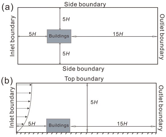
Figure 1.
Schematic of computational domains used in CFD studies: (a) top view and (b) side view.
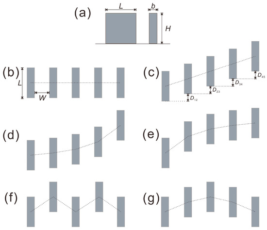
Figure 2.
Schematic of various building arrangements. (a) single building side views, (b) linear, (c) incline, (d) convex, (e) concave, (f) M-shape, and (g) V-shape arrangements.

Table 1.
Parameter settings of all cases.
The symmetry condition was set at the top and side boundaries of the domain, implying that no vertical gradient occurred for any of the parameters. The no-slip condition with standard wall functions was used for the ground and surfaces of buildings. The adopted atmospheric boundary layer profile already incorporates the effects of ground roughness. Thus, the ground and building surface roughness were ignored in this simulation. Zero-normal gradients were imposed for all flow variables at the outlet boundary.
The inlet wind speed boundary conditions are expressed as follows:
where is the velocity at the reference height, is the wind velocity, is the reference height, and α is the power-law exponent determined by the terrain category. We obtained the fitting values = 1000 mm, = 7.84 m/s, and α = 0.25 from the wind tunnel experimental data (Figure 3c). The inlet turbulent kinetic energy boundary conditions are expressed in (Figure 3d). The following equation was applied to determine the turbulence dissipation rate profiles as the inlet airflow condition:
where is the turbulent kinetic energy and is the turbulent dissipation rate. Here, was obtained from the wind tunnel experiment (Figure 3d), which was determined by measuring instantaneous velocity at high frequency and processing the data computationally, while = 0.09 is a model constant.
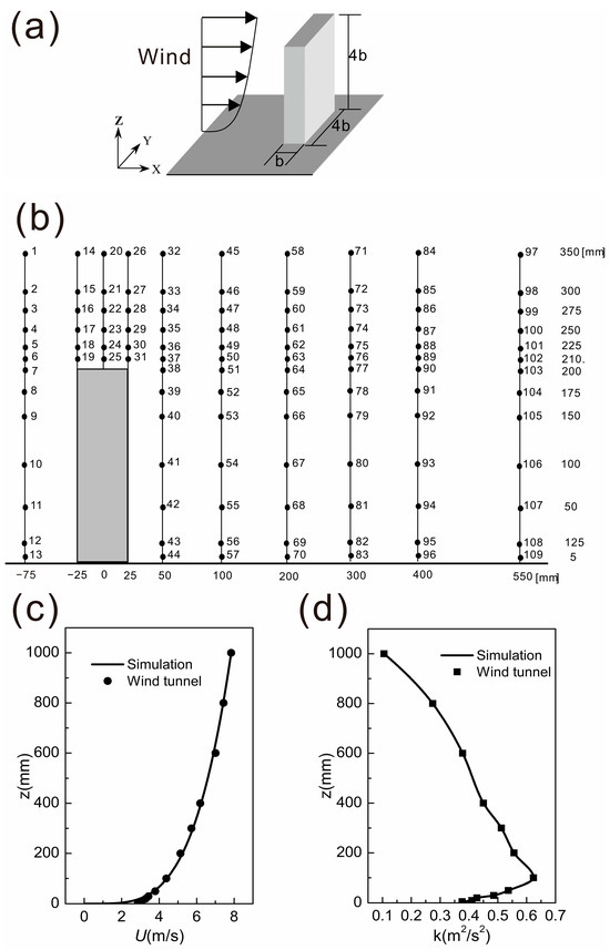
Figure 3.
Description of the wind tunnel test model. (a) 4:4:1 building, (b) location of measuring points, (c) inlet wind profile of the streamwise wind velocity, (Points: observed data, Line: theoretical fitting curve), and (d) inlet profile of turbulent kinetic energy, (Points: observed data, Line: theoretical fitting curve).
2.2. Computational Meshes
Unstructured tetrahedral meshes were generated. Regions nearer to the buildings and ground had smaller grids, and regions farther away from the buildings and ground had larger grids to save computational time. The size of the smallest mesh elements was approximately 0.075H, whereas the size of the largest mesh elements was approximately 0.4H. A prism layer mesh comprising 5 layers was applied to resolve the near-wall region. The y+ values on the critical building surfaces consistently <1. This confirms that the mesh resolution at the walls is commensurate with the employed no-slip wall treatment, ensuring the accuracy of the near-wall flow prediction. The total number of grids was approximately 1.2 million, with slight differences between various cases. For details, see Figure A1 and Table A1.
Figure 4 displays the grid-independent test results. The data used for comparison were obtained from a straight line (coordinates: (x, y, z) = (1400 mm, 800 mm to 1500 mm, 100 mm)) in the case 3. Three types of meshes (coarse, medium, and fine) were compared. The number of mesh cells for each case is shown in Table A1. The results revealed that the difference between the medium and fine grid was small, whereas the difference between the medium and coarse grid was large. Thus, about 1.2 million grids were sufficient for simulation.
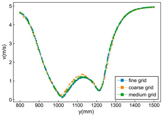
Figure 4.
Grid-independent test results.
2.3. Solution Method and Model Validation
The standard k–ε model and realizable k–ε model were simulated using COMSOL Multiphysics 5.4 software. The prediction results of these two models with the wind tunnel data are presented in Figure 5. We determined that the standard k–ε model result was a little bit closer to the wind tunnel data. Therefore, we selected the standard k–ε model to perform our simulations. The solver setup is steady and the velocity–pressure coupling is based on the “SIMPLEC” algorithm. The considered convergence criterion is 10−4. The minimal Reynolds number is about 20,000, which is much larger than 4000. So, our models can ensure Reynolds number independence.
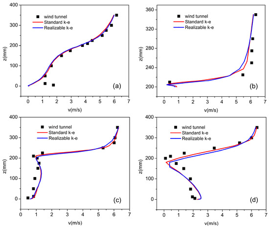
Figure 5.
Simulation and wind tunnel test velocity for the lines (a) x = −75 mm, (b) x = 0 mm, (c) x = 50 mm, and (d) x = 200 mm.
To verify the validity of our numerical simulation, we compared the results of the wind tunnel test performed at AIJ with those of our numerical simulation. The specific wind tunnel test data can be found in Supplementary Materials. Figure 3 displays the wind tunnel test model. The building width b was 50 mm in the wind tunnel test. Figure 3c,d display the inlet wind profile of the streamwise wind velocity and turbulent kinetic energy. The wind velocity and turbulent kinetic energy we used in our simulation were the same as the wind tunnel data. In Figure 5, The standard k–ε model achieved a little bit better results than the realizable model did in this case, which may be attributed to the better numerical stability of the standard k–ε model in situations where anisotropic flow is not pronounced. While the realizable model is more advanced, the standard k–ε model has its own unique advantages: robustness, good convergence, and low computational cost. Although a small difference was observed between the wind tunnel test and simulation results in the near-surface area (a maximum error of approximately 0.7 m/s was observed above pedestrian level), the results exhibited strong agreement for other areas. The trend of wind speed in the numerical simulation was consistent with that in the wind tunnel test, which indicated that the numerical model can satisfactorily predict conditions of the wind speed field.
3. Results and Discussion
The wind velocity change rate is a ventilation index denoting the dimensionless velocity magnitude and is calculated as follows:
where is the wind velocity and is the reference wind speed, which is 7.84 m/s. Here, denotes the difference between the wind speed in the inter-building space and the reference wind speed. Because the wind speed in the inter-building space is always lower than the reference speed, a bigger || value corresponds to a lower wind speed in the inter-building space.
The average wind velocity (m/s) of the middle section of inter-building space is a factor for inter-building space ventilation and is defined as follows:
where is the sectional area of the middle of inter-building space (see Table 2). This parameter indicates the average speed of the middle section of inter-building space. We calculated every of inter-building space in all cases. The results are displayed in Table 2. Here, vst.1 vst.2 vst.3 vst.4 are the average wind speed of the first, second, third, and fourth inter-building space, respectively. The magnitude and uniformity of wind speed between buildings for each case can be evaluated from the data presented in Table 2.
Table 2.
(m/s) of the inter-building spaces of 13 cases.
3.1. Effects of Building Arrangement
We studied the effects of building arrangement in cases 3, 7, 9, and 13; cases 5, 8, and 10; and cases 2, 11, and 12. Each case set had the same inter-building space width and offset. Figure 6 presents the vertical view of the contours of the predicted wind velocity change rate of four cases at z = 2b. We compared the incline, convex, concave, and M-shape arrangements. Figure 6a,c show a uniform distribution for the wind speed of the inter-building space, whereas Figure 6b reveals that the wind speed in the fourth inter-building space was considerably higher than that in other spaces. Figure 6d displays that the wind speed in the first and second space was considerably higher than that in other spaces. Figure 7 shows the contours of the predicted wind velocity change rate of three cases at z = 2b from the vertical view. We compared the incline, convex, and concave arrangements. The wind speed was almost the same for the spaces in Figure 7c but differed considerably for those in Figure 7b. The wind speed was low for the first and second spaces. Figure 8 displays the contours of the predicted wind velocity change rate of three cases at z = 2b from the vertical view. We compared the incline, M-shape, and V-shape arrangements. The difference between them was small. Figure 9 displays a comparison of among all inter-building spaces of various building arrangement cases. Cases 9 and 13 exhibited a higher average wind speed (Figure 9a), but the wind speed distribution in case 9 was more even. Cases 5 and 10 exhibited a higher average wind speed (Figure 9b), but the wind speed distribution of case 10 was more even. Cases 11 and 12 exhibited a high but nearly equal average wind speed (Figure 9c). Thus, the concave arrangement was better than the V-shape arrangement, the V-shape arrangement was better than the incline arrangement, the incline arrangement was better than the convex arrangement, and the M-shape and V-shape arrangements were equally better than the incline arrangement. Therefore, the concave arrangement was the best.
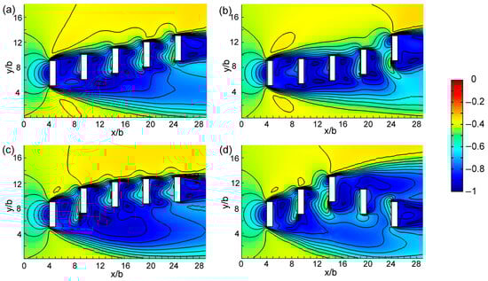
Figure 6.
Contours of the predicted wind velocity change rate (dimensionless) of four cases at z = 2b from the vertical view. (a) case 3, (b) case 7, (c) case 9, (d) case 13.
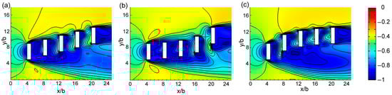
Figure 7.
Contours of the predicted wind velocity change rate (dimensionless) of three cases at z = 2b from the vertical view. (a) case 5, (b) case 8, (c) case 10.
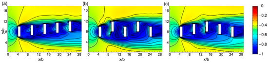
Figure 8.
Contours of the predicted wind velocity change rate (dimensionless) of three cases at z = 2b from the vertical view. (a) case 2, (b) case 11, (c) case 12.
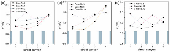
Figure 9.
Comparison of (m/s) among all inter-building spaces for (a) cases 3, 7, 9 and 13, (b) cases 5, 8, and 10, and (c) cases 2, 11, and 12.
3.2. Effects of the Offset
We studied three groups of cases, namely cases 1, 2, 3, and 4; cases 5 and 6; and cases 12 and 13, to investigate the effects of building offset. All cases in a group had the same inter-building space width and building arrangement. Among these cases, cases 4, 6, and 13 had a large building offset, whereas cases 1, 5, and 12 had a small building offset. Figure 10 displays the vertical view of the contours of the predicted wind velocity change rate of cases 1, 2, 3, and 4 at z = 2b. A larger offset corresponded to a larger high-speed region in the inter-building space. Figure 11 presents a vertical view of the contours of the predicted wind velocity change rate of cases 5 and 6 at z = 2b. The wind speed of inter-building space was higher in case 6 than in case 5. Figure 12 displays the vertical view of the contours of the predicted wind velocity change rate of cases 12 and 13 at z = 2b. Similarly, the wind speed in inter-building space was higher in case 13 than in case 12. Figure 13 presents a comparison of of all inter-building space for various building offset cases. The results indicate that larger offset results in higher average wind speed. Thus, a large offset is propitious to inter-building space ventilation.
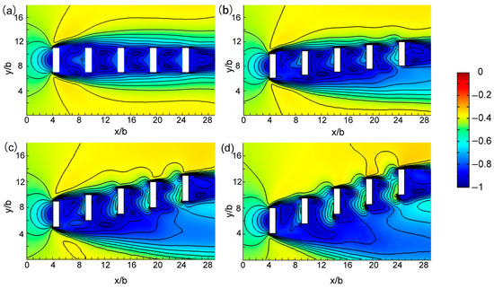
Figure 10.
Contours of the predicted wind velocity change rate (dimensionless) of four cases at z = 2b from the vertical view. (a) case 1, (b) case 2, (c) case 3, and (d) case 4.
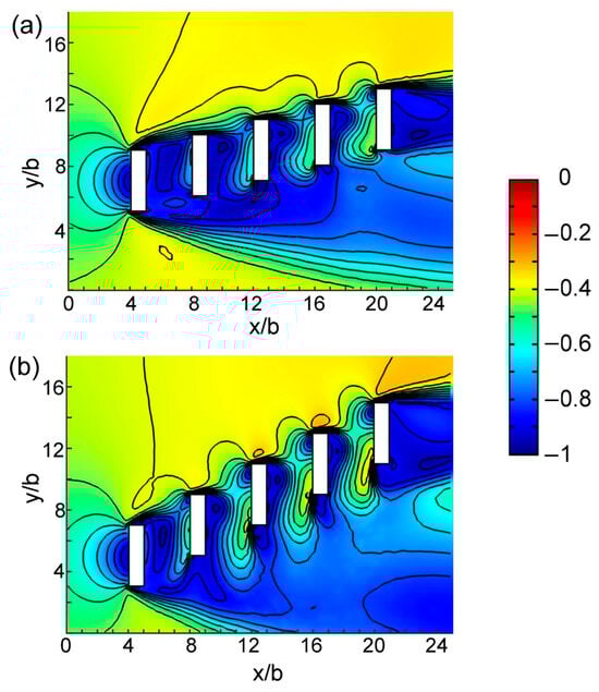
Figure 11.
Contours of the predicted wind velocity change rate (dimensionless) of two cases at z = 2b from the vertical view. (a) Case 5, (b) case 6.
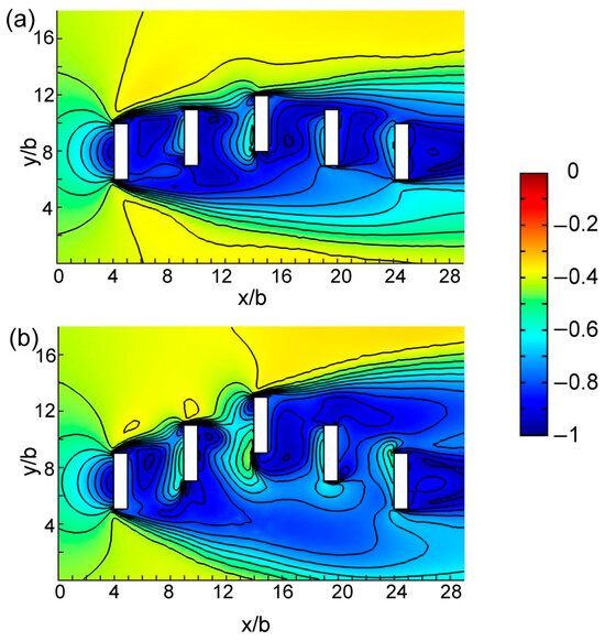
Figure 12.
Vertical view of the contours of the predicted wind velocity change rate (dimensionless) of two cases at z = 2b. (a) Case 12, (b) case 13.
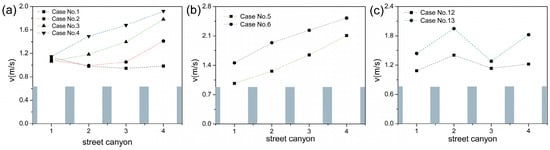
Figure 13.
(m/s) of the inter-building spaces of (a) cases 1, 2, 3, and 4, (b) cases 5 and 6, and (c) cases 12 and 13.
3.3. Urban Planning Proposals: Taking Wuhan Tianhe Meteorological Station as a Case Study
We collected wind direction data from Wuhan Tianhe Meteorological Station between 1 June and 30 September 2024, and compiled it into the wind rose diagram shown in Figure 14a. The diagram reveals that the dominant summer wind directions in this area are predominantly SSW and S, while winds from the WNW and NW directions are notably scarce. Consequently, we propose the building layout recommendations illustrated in Figure 14b,c. This design can effectively channel the prevailing summer winds through the building clusters while enhancing wind speeds between structures when the wind direction is perpendicular to building orientations.
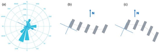
Figure 14.
(a) Wind rose diagram from Wuhan Tianhe Meteorological Station; design recommendations for suburban residential buildings: (b) concave arrangement, (c) V shape arrangement.
4. Conclusions
Thirteen cases were numerically simulated to investigate the effects of building arrangement on inter-building wind speed fields. Our analysis yielded the following conclusions:
- The concave arrangement outperforms V-shaped layouts; both M-shaped and V-shaped configurations are superior to inclined layouts, which in turn surpass convex arrangements. Thus, the concave arrangement is optimal.
- Larger offsets increase inter-building space breathability, as a result of wind flow entering the inter-building more easily.
- For the area surrounding Wuhan Tianhe Meteorological Station, we propose concave and V-shaped arrangements oriented along the WNW-ESE axis as suitable suburban configurations.
This numerical approach can be referenced to suburban residential building design to improve inter-building wind speed. The orientation of building clusters can be adjusted according to the local wind rose diagram.
Supplementary Materials
The following supporting information can be downloaded at: https://www.mdpi.com/article/10.3390/sym17101699/s1, Supplementary Data S1: Wind tunnel test data.
Author Contributions
Conceptualization, X.Y.; methodology, X.Y.; software, X.Y.; validation, X.Y.; writing—original draft preparation, X.Y.; writing—review and editing, S.Z.; visualization, X.Y.; supervision, X.Y.; funding acquisition, S.Z. All authors have read and agreed to the published version of the manuscript.
Funding
This research was funded by the National Natural Science Foundation of China, grant numbers 42074176, U1939204.
Data Availability Statement
All data, models, or code generated or used during the study are available from the corresponding author by reasonable request.
Conflicts of Interest
The authors declare no conflicts of interest.
Appendix A
The appendix illustrates the overall grid distribution and the total cell count of each model.

Figure A1.
An examples of grid arrangements (case 5).
Table A1.
The number of grid cells corresponding to each model.
Table A1.
The number of grid cells corresponding to each model.
| Case | 1 | 2 | 3 | 4 | 5 | 6 | 7 | 8 |
| Grid number | 1,261,016 | 1,238,447 | 1,224,506 | 1,203,714 | 1,161,137 | 1,133,866 | 1,226,298 | 1,164,262 |
| Case | 9 | 10 | 11 | 12 | 13 | Coarse | Medium | Fine |
| Grid number | 1,224,475 | 1,163,513 | 1,229,937 | 1,223,598 | 1,189,853 | 207,513 | 1,224,506 | 4,592,660 |
References
- Makvandi, M.; Li, W.; Ou, X.; Chai, H.; Khodabakhshi, Z.; Fu, J.; Yuan, P.F.; Horimbere, E.d.l.J. Urban Heat Mitigation towards Climate Change Adaptation: An Eco-Sustainable Design Strategy to Improve Environmental Performance under Rapid Urbanization. Atmosphere 2023, 14, 638. [Google Scholar] [CrossRef]
- He, B.J. Towards the next generation of green building for urban heat island mitigation: Zero UHI impact building. Sustain. Cities Soc. 2019, 50, 101647. [Google Scholar] [CrossRef]
- Sasaki, Y.; Matsuo, K.; Yokoyama, M.; Sasaki, M.; Tanaka, T.; Sadohara, S. Sea breeze effect mapping for mitigating summer urban warming: For making urban environmental climate map of Yokohama and its surrounding area. Urban Clim. 2018, 24, 529–550. [Google Scholar] [CrossRef]
- Chen, X.; Kang, H.; Zhao, J.; Liu, Q. Optimization Design Research of Architectural Layout and Morphology in Multi-Story Dormitory Areas Based on Wind Environment Analysis. Buildings 2025, 15, 1747. [Google Scholar] [CrossRef]
- Zhou, Y.; Guan, H.; Huang, C.; Fan, L.; Gharib, S.; Batelaan, O.; Simmons, C. Sea breeze cooling capacity and its influencing factors in a coastal city. Build. Environ. 2019, 166, 106408. [Google Scholar] [CrossRef]
- Niu, J.; Liu, J.; Lee, T.C.; Lin, Z.J.; Mak, C.; Tse, K.T.; Tang, B.; Kwok, K.C. A new method to assess spatial variations of outdoor thermal comfort: Onsite monitoring results and implications for precinct planning. Build. Environ. 2015, 91, 263–270. [Google Scholar] [CrossRef]
- Li, J.; Liu, N. The perception, optimization strategies and prospects of outdoor thermal comfort in China: A review. Build. Environ. 2020, 170, 106614. [Google Scholar] [CrossRef]
- Ng, E. Policies and technical guidelines for urban planning of high-density cities—Air ventilation assessment (AVA) of Hong Kong. Build. Environ. 2009, 44, 1478–1488. [Google Scholar] [CrossRef] [PubMed]
- Mills, G. Urban climatology: History, status and prospects. Urban Clim. 2014, 10, 479–489. [Google Scholar] [CrossRef]
- Fu, J.Y.; Wu, J.R.; Xu, A.; Li, Q.S.; Xiao, Y.Q. Full-scale measurements of wind effects on Guangzhou West Tower. Eng. Struct. 2012, 35, 120–139. [Google Scholar] [CrossRef]
- Li, Q.S.; Fang, J.Q.; Jeary, A.P.; Wong, C.K. Full scale measurements of wind effects on tall buildings. J. Wind Eng. Ind. Aerodyn. 1998, 74–76, 741–750. [Google Scholar] [CrossRef]
- Yang, L.; Li, Y. City ventilation of Hong Kong at no-wind conditions. Atmos. Environ. 2009, 43, 3111–3121. [Google Scholar] [CrossRef]
- Baker, C.J. The theory of flow between two buildings—Experimental verification of the assumptions of Britter and Hunt’s theory. J. Wind Eng. Ind. Aerodyn. 1980, 6, 169–174. [Google Scholar] [CrossRef]
- Britter, R.E.; Hunt, J.C.R. Velocity measurements and order of magnitude estimates of the flow between two buildings in a simulated atmospheric boundary layer. J. Ind. Aerodn. 1979, 4, 165–182. [Google Scholar] [CrossRef]
- Tanaka, H.; Tamura, Y.; Ohtake, K. Experimental investigation of aerodynamic forces and wind pressures acting on tall buildings with various unconventional arrangements. J. Wind Eng. Ind. Aerodyn. 2012, 107, 179–191. [Google Scholar] [CrossRef]
- Meena, R.K.; Raj, R.; Anbukumar, S.; Khan, M.I.; Khatib, J.M. Fluid Dynamic Assessment of Tall Buildings with a Variety of Complicated Geometries. Buildings 2024, 14, 4081. [Google Scholar] [CrossRef]
- Blocken, B. 50 years of computational wind engineering: Past, present and future. J. Wind Eng. Ind. Aerodyn. 2014, 129, 69–102. [Google Scholar] [CrossRef]
- Du, Y.; Mak, C.M.; Liu, J. Effects of lift-up design on pedestrian level wind comfort in different building arrangements under three wind directions. Build. Environ. 2017, 117, 84–99. [Google Scholar] [CrossRef]
- Du, Y.; Mak, C.M.; Tang, B.S. Effects of building height and porosity on pedestrian level wind comfort in a high-density urban built environment. Build. Simul. 2018, 11, 1215–1228. [Google Scholar] [CrossRef]
- Li, Y.; Chen, L. Study on the influence of voids on high-rise building on the wind environment. Build. Simul. 2019, 13, 419–438. [Google Scholar] [CrossRef]
- Mochida, A.; Tominaga, Y.; Yoshie, R. AIJ Guideline for Practical Applications of CFD to Wind Environment around Buildings. J. Wind Eng. Ind. Aerodyn. 2006, 95, 533–536. [Google Scholar]
- Mei, S.J.; Luo, Z.; Zhao, F.Y.; Wang, H. Street canyon ventilation and pollution dispersion: 2-D versus 3-D CFD simulations. Sustain. Cities Soc. 2019, 50, 101700. [Google Scholar] [CrossRef]
- Chao, Y.; Ng, E. Building porosity for better urban ventilation in high-density cities—A computational parametric study. Build. Environ. 2012, 50, 176–189. [Google Scholar]
- Chen, L.; Hang, J.; Sandberg, M.; Claesson, L.; Di Sabatino, S.; Wigo, H. The impacts of building height variations and building packing densities on flow adjustment and city breathability in idealized urban models. Build. Environ. 2017, 118, 344–361. [Google Scholar] [CrossRef]
- Hang, J.; Li, Y.G. Ventilation strategy and air change rates in idealized high-rise compact urban areas. Build. Environ. 2010, 45, 2754–2767. [Google Scholar] [CrossRef]
- Hunter, L.J.; Johnson, G.T.; Watson, I.D. An Investigation of 3-dimensional characteristics of flow regimes within the urban canyon. Atmos. Environ. 1992, 26, 425–432. [Google Scholar] [CrossRef]
- You, Y.; Yu, F.; Mao, N. Fast Prediction and Optimization of Building Wind Environment Using CFD and Deep Learning Method. Appl. Sci. 2024, 14, 4087. [Google Scholar] [CrossRef]
- Oke, T.R. Street design and urban canopy layer climate. Energy Build. 1988, 11, 103–113. [Google Scholar] [CrossRef]
- Wong, M.S.; Nichol, J.; Ng, E. A study of the “wall effect” caused by proliferation of high-rise buildings using GIS techniques. Landsc. Urban Plan. 2011, 102, 245–253. [Google Scholar] [CrossRef]
- Yim, S.H.L.; Fung, J.C.H.; Lau, A.K.H.; Kot, S.C. Air ventilation impacts of the “wall effect” resulting from the alignment of high-rise buildings. Atmos. Environ. 2009, 43, 4982–4994. [Google Scholar] [CrossRef]
- Silva, P.U.d.; Bono, G.; Greco, M. Assessing Pedestrian Comfort in Dense Urban Areas Using CFD Simulations: A Study on Wind Angle and Building Height Variations. Fluids 2025, 10, 233. [Google Scholar] [CrossRef]
- Wen, C.Y.; Juan, Y.H.; Yang, A.S. Enhancement of city breathability with half open spaces in ideal urban street canyons. Build. Environ. 2017, 112, 322–336. [Google Scholar] [CrossRef]
- Aristodemou, E.; Boganegra, L.M.; Mottet, L.; Pavlidis, D.; Constantinou, A.; Pain, C.; Robins, A.; Apsimon, H. How tall buildings affect turbulent air flows and dispersion of pollution within a neighbourhood. Environ. Pollut. 2018, 233, 782–796. [Google Scholar] [CrossRef]
- Gu, Z.L.; Zhang, Y.W.; Cheng, Y.; Lee, S.C. Effect of uneven building layout on air flow and pollutant dispersion in non-uniform street canyons. Build. Environ. 2011, 46, 2657–2665. [Google Scholar] [CrossRef]
- Buccolieri, R.; Sandberg, M.; Di Sabatino, S. City breathability and its link to pollutant concentration distribution within urban-like geometries. Atmos. Environ. 2010, 44, 1894–1903. [Google Scholar] [CrossRef]
- Chang, C.H.; Meroney, R.N. Concentration and flow distributions in urban street canyons: Wind tunnel and computational data. J. Wind Eng. Ind. Aerodyn. 2003, 91, 1141–1154. [Google Scholar] [CrossRef]
- Razak, A.A.; Hagishima, A.; Ikegaya, N.; Tanimoto, J. Analysis of airflow over building arrays for assessment of urban wind environment. Build. Environ. 2013, 59, 56–65. [Google Scholar] [CrossRef]
- Zhang, X.; Tse, K.T.; Weerasuriya, A.U.; Kwok, K.C.S.; Niu, J.; Lin, Z. Evaluation of pedestrian wind comfort near ‘lift-up’ buildings with different aspect ratios and central core modifications. Build. Environ. 2017, 124, 245–257. [Google Scholar] [CrossRef]
- Hang, J.; Luo, Z.; Sandberg, M.; Gong, J. Natural Ventilation Assessment in Typical Open and Semi-Open Urban Environments Under Various Wind Directions. Build. Environ. 2013, 70, 318–333. [Google Scholar] [CrossRef]
- Wan, I.W.H.; Mohamad, M.F.; Abd Razak, A.; Ikegaya, N.; Chung, J.; Hirose, C.; Mohd Azmi, A. Comprehensive Comparisons of RANS, LES, and Experiments over Cross-Ventilated Building under Sheltered Conditions. Build. Environ. 2024, 254, 111402. [Google Scholar] [CrossRef]
- Santiago, J.L.; Dejoan, A.; Martilli, A.; Martin, F.; Pinelli, A. Comparison between Large-Eddy Simulation and Reynolds-Averaged Navier–Stokes Computations for the MUST Field Experiment. Part I: Study of the Flow for an Incident Wind Directed Perpendicularly to the Front Array of Containers. Bound. Layer Meteorol. 2010, 135, 109–132. [Google Scholar] [CrossRef]
- Salim, S.M.; Buccolieri, R.; Chan, A.; Di Sabatino, S. Numerical Simulation of Atmospheric Pollutant Dispersion in an Urban Street Canyon: Comparison between RANS and LES. J. Wind Eng. Ind. Aerodyn. 2011, 99, 103–113. [Google Scholar] [CrossRef]
- Strasszer, D.; Xydis, G. CFD-Based Wind Assessment for Suburban Buildings: The Case Study of Aarhus University, Herning Campus. Front. Energy Res. 2020, 8, 539095. [Google Scholar] [CrossRef]
- Hnaien, N.; Hassen, W.; Kolsi, L.; Mesloub, A.; Alghaseb, M.A.; Elkhayat, K.; Abdelhafez, M.H.H. CFD Analysis of Wind Distribution around Buildings in Low-Density Urban Community. Mathematics 2022, 10, 1118. [Google Scholar] [CrossRef]
- Yoshie, R.; Mochida, A.; Tominaga, Y.; Kataoka, H.; Harimoto, K.; Nozu, T.; Shirasawa, T. Cooperative project for CFD prediction of pedestrian wind environment in the Architectural Institute of Japan. J. Wind Eng. Ind. Aerodyn. 2007, 95, 1551–1578. [Google Scholar] [CrossRef]
- Tominaga, Y.; Mochida, A.; Murakami, S.; Sawaki, S. Comparison of various revised k–ε models and LES applied to flow around a high-rise building model with 1:1:2 shape placed within the surface boundary layer. J. Wind Eng. Ind. Aerodyn. 2008, 96, 389–411. [Google Scholar] [CrossRef]


Disclaimer/Publisher’s Note: The statements, opinions and data contained in all publications are solely those of the individual author(s) and contributor(s) and not of MDPI and/or the editor(s). MDPI and/or the editor(s) disclaim responsibility for any injury to people or property resulting from any ideas, methods, instructions or products referred to in the content. |
© 2025 by the authors. Licensee MDPI, Basel, Switzerland. This article is an open access article distributed under the terms and conditions of the Creative Commons Attribution (CC BY) license (https://creativecommons.org/licenses/by/4.0/).