An Explicit Positivity-Preserving Method for Nonlinear Aït-Sahalia Model Driven by Fractional Brownian Motion

Abstract

This paper develops an explicit positivity-preserving method for the nonlinear Aït-Sahalia interest rate model driven by fractional Brownian motion. To overcome the difficulties in obtaining the convergence rate of this positivity-preserving method, the Lamperti transformation is utilized, which gives an auxiliary equation. And the convergence rate of the numerical method for this auxiliary equation is obtained by virtue of Malliavin calculus. Naturally, the target follows from the inverse of the Lamperti transformation. As a byproduct, the convergence rate of the explicit positivity-preserving method for stochastic differential equations driven by fractional Brownian motion with symmetric coefficients is obtained. Finally, several numerical experiments are performed to verify the theoretical results and demonstrate the advantage of the explicit method.

1. Introduction

Based on the exploration of some continuous-time interest rate models, the well-known Aït-Sahalia interest rate model (ASIRM) was proposed in [1], which was extensively employed in the quantitative analysis of real financial markets [2,3]. Given its application value, many scholars have analyzed the ASIRM. In addition, due to the difficulty in obtaining analytical solutions, the necessity of a numerical method for ASIRM is evident. Assuming the nonlinear ASIRM is driven by standard Brownian motion, the backward Euler–Maruyama (EM) method [4], the truncated EM method [5], and the positivity-preserving method [6,7] have been discussed. And stochastic differential equations (SDEs) with irregular coefficients are studied in [8,9,10]. Moreover, for both theoretical and practical reasons, modeling the dynamics of interest rates and asset prices is crucial for analyzing and understanding their characteristics [11,12,13].

In light of the memory impact of fractional Brownian motion (FBM) on models, which often appears in the real market, it is more meaningful to investigate financial models driven by FBM [14,15]. This investigation enhances our ability to characterize the complex behavior of financial markets. Similarly, fractional-order systems provide a powerful framework for modeling dynamical systems [16]. Thus, in this paper, we focus on the numerical methods for nonlinear scalar ASIRM driven by FBM of the following form:

$$d{X}_t=\left(a_{-1}{X}_t^{-1}-a_0+a_1{X}_t-a_2{X}_t^{\eta }\right)dt+\sigma X_t^{\lambda }d{B}_t^H,t\in [0,T],$$

(1)

with the initial value $X_0>0$, where $\eta +1>2\lambda$, $\eta \ge 2\wedge \lambda +1>2$, and $a_{-1},a_0,a_1,a_2,\sigma >0$. And $B_t^H$ is an FBM with Hurst parameter $H\in (1/2,1)$. Since the solution of ASIRM has practical significance, the development of a positivity-preserving method for (1) is of critical importance. The well-posedness of ASIRM (1) was studied in [17], and the implicit numerical method was also applied, without presenting numerical simulations. Moreover, it should also be noted that the Cox–Ingersoll–Ross models driven by FBM have been approximated using the backward EM method [18] and truncated EM method [19], which guarantee the positivity of the numerical solutions. The theories of SDEs driven by FBM have been investigated in [20,21,22,23,24]. For work about fractional analysis, see [25,26].

Motivated by [17,27], in this paper, we utilize the positivity-preserving method to approximate the ASIRM driven by FBM. As an explicit numerical method, it offers distinct advantages over the implicit EM method in [17], like easy implementation and more relaxed constraints on step size. We compare its runtime with that of the backward EM method through numerical simulations in Section 5. In contrast to standard Brownian motion, analyzing SDEs driven by FBM presents two fundamental challenges: the dependence between increments and the absence of the martingale property. To overcome the challenges, we first use the Lamperti transformation to show the corresponding auxiliary Equation (2), and construct the numerical method for this auxiliary equation. Then, a strong convergence rate is obtained by Malliavin calculus. Next, the strong convergence rate of the positivity-preserving method for ASIRM (1) is achieved by virtue of the inverse of the Lamperti transformation, which is dependent on the Hurst parameter H.

The paper is structured as follows. Some notations and necessary lemmas are presented in Section 2. After using the Lamperti transformation, the positivity-preserving method for auxiliary Equation (2) is studied in Section 3. Then, the strong convergence of the positivity-preserving method for ASIRM (1) is established by exploiting the inverse of the Lamperti transformation in Section 4. In Section 5, several numerical simulations are demonstrated to verify the theories.

2. Preliminaries

Let $\left(\mathrm{\Omega },\mathcal{F},\mathbb{P}\right)$ be a filtered probability space satisfying the usual conditions. Denote $B^H=\{B_t^H,t\in [0,T]\}$ by a one-dimensional FBM with Hurst parameter $H\in ({\displaystyle \frac{1}{2}},1)$ defined on $\left(\mathrm{\Omega },\mathcal{F},\mathbb{P}\right)$, i.e., $B^H$ is a Gaussian process centered on the covariance function

$$\mathbb{E}\left(B_t^H{B}_s^H\right)=R_H(t,s)={\displaystyle \frac{1}{2}}\left(t^{2H}+s^{2H}-{|t-s|}^{2H}\right).$$

Moreover, one can see that $\mathbb{E}|B_t^H-B_s^H{|}^p=C_p{|t-s|}^{pH}$ for all $p\ge 1$. For each $t\in [0,T]$, let ${\mathcal{F}}_t$ be the $\sigma$-algebra generated by the random variables $\{B_s^H:s\in [0,t]\}$ and the null sets. The stochastic integral of FBM in this paper is defined through the techniques of fractional calculus developed by Zähle in [28], under which (1) is regarded as a pathwise Riemann–Stieltjes integral equation.

For any $a,b\in \mathbb{R}$, let $a\wedge b=min\{a,b\}$ and $a\vee b=max\{a,b\}$. For a set S, let ${\mathbb{I}}_S(x)=1$ if $x\in S$ and 0 otherwise. Let C be a suitable constant independent of the step size $\Delta$. Let $\mathcal{E}$ be the set of step functions on $[0,T]$. Denote by $\mathcal{H}$ the Hilbert space defined as the closure of $\mathcal{E}$ with respect to the scalar product

$$c_H{\int }_0^T{\int }_0^T{\mathbb{I}}_{[0,t]}(u){\mathbb{I}}_{[0,s]}(v){|u-v|}^{2H-2}dudv,$$

where $c_H=H(2H-1)$. Let

$$|\mathcal{H}|=\left\{\psi \in {\mathcal{H}|\parallel \psi \parallel }_{|\mathcal{H}|}^2=c_H{\int }_0^T{\int }_0^T{|\psi (s)||\psi (t)||t-s|}^{2H-2}dsdt<\infty \right\}$$

and $|\mathcal{H}|\otimes |\mathcal{H}|$ be the set of all measurable function such that

$${\parallel \psi \parallel }_{|\mathcal{H}|\otimes |\mathcal{H}|}^2:=c_H^2{\int }_{{[0,T]}^4}{|\psi (u,s)||\psi (v,t)||u-v|}^{2H-2}{|t-s|}^{2H-2}dudvdtds<\infty .$$

For $p>1$, we denote by ${\mathbb{D}}_{|\mathcal{H}|}^{1,p}$ all the random variables u such that $u\in |\mathcal{H}|$ a.s., its Malliavin derivative $Du\in |\mathcal{H}|\otimes |\mathcal{H}|$ a.s., and

$${\mathbb{E}\parallel u\parallel }_{|\mathcal{H}|}^p+\mathbb{E}{\parallel Du\parallel }_{|\mathcal{H}|\otimes |\mathcal{H}|}^p<\infty .$$

We now show the following lemma connecting the stochastic integral about FBM with the Skorohod integral $\int ·\delta B^H$; see [29,30].

Lemma 1. 

Let ${\left\{u_t\right\}}_{t\in [0,T]}$ be a stochastic process in ${\mathbb{D}}_{|\mathcal{H}|}^{1,2}$ with $H>{\displaystyle \frac{1}{2}}$ such that a.s.

$${\int }_0^T{\int }_0^T|D_s{u}_t{||t-s|}^{2H-2}dtds<\infty .$$

Then,

$${\int }_0^T{u}_{t}d{B}_t^H={\int }_0^T{u}_t\delta B_t^H+c_H{\int }_0^T{\int }_0^T{D}_s{u}_t{|t-s|}^{2H-2}dtds.$$

For $p>1/H$,

$$\mathbb{E}\left(\underset{t\in [0,T]}{sup}{|{\int }_0^t{u}_s\delta B_s^H|}^p\right)\le C\left(\mathbb{E}{\int }_0^T{|u_s|}^{p}ds+\mathbb{E}{\int }_0^T{\left({\int }_0^T{|D_r{u}_s|}^{1/H}dr\right)}^{pH}ds\right).$$

We now describe some conclusions from [17] as the following lemma.

Lemma 2. 

Under the given conditions on parameters, ASIRM (1) possesses a unique solution $Y_t\in \mathcal{C}\left([0,T],(0,\infty )\right)$. For any $p>0$, we have

$$\mathbb{E}\underset{0\le t\le T}{sup}{X}_t^{-p}<\infty ,\mathbb{E}\underset{0\le t\le T}{sup}{X}_t^p<\infty .$$

Then, the Lamperti transformation $Y_t=X_t^{1-\lambda }$ for (2) leads to an auxiliary equation:

$$d{Y}_t=(\lambda -1)\left[a_2{Y}_t^{-{\displaystyle \frac{\eta -\lambda }{\lambda -1}}}-a_1{Y}_t+a_0{Y}_t^{{\displaystyle \frac{\lambda }{\lambda -1}}}-a_{-1}{Y}_t^{{\displaystyle \frac{\lambda +1}{\lambda -1}}}\right]dt+\sigma (1-\lambda )d{B}_t^H,$$

(2)

with the initial value $Y_0=X_0^{1-\lambda }$. Obviously, the conclusions in Lemma 2 also hold for (2). For simplicity, define

$$\mu (y)=(\lambda -1)\left(a_2{y}^{-{\displaystyle \frac{\eta -\lambda }{\lambda -1}}}-a_{1}y+a_0{y}^{{\displaystyle \frac{\lambda }{\lambda -1}}}-a_{-1}{y}^{{\displaystyle \frac{\lambda +1}{\lambda -1}}}\right).$$

(3)

Thus, we know that

$${\mu }^{\prime }(y)=a_2(-\eta +\lambda )y^{-{\displaystyle \frac{\eta -1}{\lambda -1}}}-a_1(\lambda -1)+a_0\lambda y^{{\displaystyle \frac{1}{\lambda -1}}}-a_{-1}(\lambda +1)y^{{\displaystyle \frac{2}{\lambda -1}}},$$

(4)

$${\mu }^{″}(y)=a_2(-\eta +\lambda )(-{\displaystyle \frac{\eta -1}{\lambda -1}})y^{-{\displaystyle \frac{\eta +\lambda -2}{\lambda -1}}}+a_0{\displaystyle \frac{\lambda }{\lambda -1}}{y}^{{\displaystyle \frac{2-\lambda }{\lambda -1}}}-a_{-1}{\displaystyle \frac{2(\lambda +1)}{\lambda -1}}{y}^{{\displaystyle \frac{3-\lambda }{\lambda -1}}}.$$

(5)

Recall a crucial equality: for $a,b\in {\mathbb{R}}_{+}$ and $\varrho \ne 1$,

$$a^{\varrho }-b^{\varrho }=\varrho (a-b){\int }_0^1{\left[(1-r)b+ra\right]}^{\varrho -1}dr.$$

(6)

By (6), we arrive at

$$\begin{array}{cc}\hfill \left|{\displaystyle \frac{n^{\frac{\eta -\lambda }{\lambda -1}}-m^{\frac{\eta -\lambda }{\lambda -1}}}{{(mn)}^{\frac{\eta -\lambda }{\lambda -1}}}}\right|& \le C{\displaystyle \frac{|m-n|\left(1+m^{\frac{\eta -\lambda }{\lambda -1}-1}+n^{\frac{\eta -\lambda }{\lambda -1}-1}\right)}{{(mn)}^{\frac{\eta -\lambda }{\lambda -1}}}}\hfill \\ \hfill & \le C\left(1+{\displaystyle \frac{1}{2m^{\frac{2(\eta -\lambda )}{\lambda -1}}}}+{\displaystyle \frac{1}{2n^{\frac{2(\eta -\lambda )}{\lambda -1}}}}\right)|m-n|,\hfill \end{array}$$

Thus, there exists a constant $L_1>0$ such that

$$\begin{array}{cc}\hfill & |\mu (m)-\mu (n)|\le L_1\left(1+{\displaystyle \frac{1}{m^{\frac{2(\eta -\lambda )}{\lambda -1}}}}+{\displaystyle \frac{1}{n^{\frac{2(\eta -\lambda )}{\lambda -1}}}}+m^{{\displaystyle \frac{2}{\lambda -1}}}+n^{{\displaystyle \frac{2}{\lambda -1}}}\right)|m-n|.\hfill \end{array}$$

(7)

From (4), we can observe that ${lim}_{y\to 0^{+}}{\mu }^{\prime }(y)={lim}_{y\to \infty }{\mu }^{\prime }(y)=-\infty .$ Due to continuity, ${sup}_{y\in (0,\infty )}{\mu }^{\prime }(y)$ is finite. Then, the drift coefficient $\mu$ is one-sided Lipschitz continuous, and we assume that this Lipschitz constant is $L_2>0$. That is, there exists a constant $L_2>0$ such that

$$\begin{array}{c}\hfill (m-n)(\mu (m)-\mu (n))\le L_2{|m-n|}^2,\forall m,n\in {\mathbb{R}}_{+}.\end{array}$$

(8)

3. Numerical Method for Auxiliary Equation (2)

In this section, we give the definition of the explicit positivity-preserving method and discuss its covergence rate. For positive integer M, the step size is denoted by $\Delta ={\displaystyle \frac{T}{M}}$. Set $t_k=k\Delta$, $k\in {\mathbb{S}}_M:=\{0,1,2,\cdots ,M\}$. Let $\Delta \in (0,1]$ and $\alpha \in (0,{\displaystyle \frac{\lambda -1}{4(\eta -\lambda )}}]$, $\beta \in (0,{\displaystyle \frac{\lambda -1}{4}}]$. The truncation mapping ${\phi }_{\Delta }:\mathbb{R}\to {\mathbb{R}}_{+}$ is defined as

$${\phi }_{\Delta }(y)=(K_1{\Delta }^{\alpha })\vee y\wedge (K_2{\Delta }^{-\beta }),$$

where $K_1$ and $K_2$ are two positive constants independent of $\Delta$ with $K_1\le Y_0$ and $K_2\ge Y_0$. Moreover, we can derive that $|{\phi }_{\Delta }(y)|\le |y|$ and $|{\phi }_{\Delta }(y_1)-{\phi }_{\Delta }(y_2)|\le C|y_1-y_2|$ for some positive constant C. Now, define the explicit positivity-preserving method as

$$Z_{k+1}=Z_k+{\mu }_{\Delta }(Z_k)\Delta +\sigma (1-\lambda )\Delta B_{k+1}^H,k\in {\mathbb{S}}_M,$$

where ${\mu }_{\Delta }(·):=\mu \left({\phi }_{\Delta }(·)\right)$ and $\Delta B_{k+1}^H=B_{t_{k+1}}^H-B_{t_k}^H$.

Remark 1. 

We get from Lemma 2.1 in [27] that ${\mu }_{\Delta }$ is Lipschitz continuous with the Lipschitz constant $L(\Delta )=2L_1\left(1+{\Delta }^{-{\displaystyle \frac{2\alpha (\eta -\lambda )}{\lambda -1}}}+{\Delta }^{-{\displaystyle \frac{2\beta }{\lambda -1}}}\right),$ and ${\mu }_{\Delta }$ is one-sided Lipschitz continuous with the Lipschitz constant $L_2$. Moreover, we see $L^2(\Delta )\Delta \le C$.

Lemma 3. 

Under the conditions of Lemma 2 with $p>\left[{\displaystyle \frac{4(\eta -\lambda )}{\lambda -1}}\vee {\displaystyle \frac{2\lambda +2}{\lambda -1}}\right]$, for any $t\in [0,T]$, we derive that

$$\mathbb{E}|\mu (Y_t)-{\mu }_{\Delta }(Y_t){|}^2\le C{\Delta }^{{\displaystyle \frac{[\alpha (p\lambda -p-4\eta +6\lambda -2)]\wedge [\beta (p\lambda -p-2\lambda -2)]}{\lambda -1}}}.$$

Proof. 

We get from (7) and the definition of ${\mu }_{\Delta }$ that

$$\begin{array}{cc}\hfill & |\mu (Y_t)-{\mu }_{\Delta }(Y_t){|}^2\hfill \\ \hfill \le & C\left(1+|Y_t{|}^{-{\displaystyle \frac{4(\eta -\lambda )}{\lambda -1}}}+|{\phi }_{\Delta }(Y_t){|}^{-{\displaystyle \frac{4(\eta -\lambda )}{\lambda -1}}}+|Y_t{|}^{{\displaystyle \frac{4}{\lambda -1}}}|+|{\phi }_{\Delta }(Y_t){|}^{{\displaystyle \frac{4}{\lambda -1}}}\right){|Y_t-{\phi }_{\Delta }(Y_t)|}^2\hfill \\ \hfill \le & C(1+|Y_t{|}^{-{\displaystyle \frac{4(\eta -\lambda )}{\lambda -1}}})|Y_t-K_1{\Delta }^{\alpha }{|}^2{\mathbb{I}}_{\{Y_t<K_1{\Delta }^{\alpha }\}}+C\left(1+|Y_t{|}^{{\displaystyle \frac{4}{\lambda -1}}}\right){|Y_t-K_2{\Delta }^{-\beta }|}^2{\mathbb{I}}_{\{Y_t>K_2{\Delta }^{-\beta }\}}\hfill \\ \hfill \le & C{\Delta }^{2\alpha }\left(1+|Y_t{|}^{-{\displaystyle \frac{4(\eta -\lambda )}{\lambda -1}}}\right){\mathbb{I}}_{\{Y_t<K_1{\Delta }^{\alpha }\}}+C\left(1+|Y_t{|}^{{\displaystyle \frac{4}{\lambda -1}}}\right){|Y_t|}^2{\mathbb{I}}_{\{Y_t>K_2{\Delta }^{-\beta }\}}.\hfill \end{array}$$

Applying Hölder’s inequality, Markov’s inequality, and Lemma 2 with $p>\left[{\displaystyle \frac{4(\eta -\lambda )}{\lambda -1}}\vee {\displaystyle \frac{2\lambda +2}{\lambda -1}}\right]$ gives that

$$\begin{array}{cc}\hfill & \mathbb{E}[\left(1+|Y_t{|}^{-{\displaystyle \frac{4(\eta -\lambda )}{\lambda -1}}}\right){\mathbb{I}}_{\{Y_t<K_1{\Delta }^{\alpha }\}}]\hfill \\ \hfill \le & C(\mathbb{P}[Y_t<K_1{\Delta }^{\alpha }]+\mathbb{E}\left[|Y_t{|}^{-{\displaystyle \frac{4(\eta -\lambda )}{\lambda -1}}}{\mathbb{I}}_{\{Y_t<K_1{\Delta }^{\alpha }\}}\right])\hfill \\ \hfill \le & C\mathbb{P}[Y_t^{-1}>K_1^{-1}{\Delta }^{-\alpha }]+C{\left[\mathbb{E}|Y_t{|}^{-p}\right]}^{{\displaystyle \frac{4(\eta -\lambda )}{p(\lambda -1)}}}{\left[\mathbb{E}{\mathbb{I}}_{\{Y_t<K_1{\Delta }^{\alpha }\}}\right]}^{1-{\displaystyle \frac{4(\eta -\lambda )}{p(\lambda -1)}}}\hfill \\ \hfill \le & C{K}_1^p{\Delta }^{p\alpha }\mathbb{E}{|Y_t|}^{-p}+C{\left[\mathbb{E}|Y_t{|}^{-p}\right]}^{{\displaystyle \frac{4(\eta -\lambda )}{p(\lambda -1)}}}{\left(\mathbb{P}[Y_t^{-1}>K_1^{-1}{\Delta }^{-\alpha }]\right)}^{1-{\displaystyle \frac{4(\eta -\lambda )}{p(\lambda -1)}}}\hfill \\ \hfill \le & C{\Delta }^{p\alpha }+C{\Delta }^{{\displaystyle \frac{\alpha (p\lambda -p-4\eta +4\lambda )}{\lambda -1}}}\hfill \\ \hfill \le & C{\Delta }^{{\displaystyle \frac{\alpha (p\lambda -p-4\eta +4\lambda )}{\lambda -1}}}.\hfill \end{array}$$

and

$$\begin{array}{cc}\hfill & \mathbb{E}\left[\left(1+|Y_t{|}^{{\displaystyle \frac{4}{\lambda -1}}}\right){|Y_t|}^2{\mathbb{I}}_{\{Y_t>K_2{\Delta }^{-\beta }\}}\right]\hfill \\ \hfill \le & \mathbb{E}\left[|Y_t{|}^2{\mathbb{I}}_{\{Y_t>K_2{\Delta }^{-\beta }\}}\right]+\mathbb{E}\left[|Y_t{|}^{{\displaystyle \frac{2\lambda +2}{\lambda -1}}}{\mathbb{I}}_{\{Y_t>K_2{\Delta }^{-\beta }\}}\right]\hfill \\ \hfill \le & {\left[\mathbb{E}|Y_t{|}^p\right]}^{{\displaystyle \frac{2}{p}}}{\left[\mathbb{E}{\mathbb{I}}_{\{Y_t>K_2{\Delta }^{-\beta }\}}\right]}^{1-{\displaystyle \frac{2}{p}}}+{\left[\mathbb{E}|Y_t{|}^p\right]}^{{\displaystyle \frac{2\lambda +2}{p(\lambda -1)}}}{\left[\mathbb{E}{\mathbb{I}}_{\{Y_t>K_2{\Delta }^{-\beta }\}}\right]}^{1-{\displaystyle \frac{2\lambda +2}{p(\lambda -1)}}}\hfill \\ \hfill \le & C{\Delta }^{p\beta (1-{\displaystyle \frac{2}{p}})}+C{\Delta }^{p\beta (1-{\displaystyle \frac{2\lambda +2}{p(\lambda -1)}})}\le C{\Delta }^{{\displaystyle \frac{\beta (p\lambda -p-2\lambda -2)}{\lambda -1}}}.\hfill \end{array}$$

Thus,

$$\begin{array}{cc}\hfill & \mathbb{E}|\mu (Y_t)-{\mu }_{\Delta }(Y_t){|}^2\hfill \\ \hfill & \le C{\Delta }^{2\alpha }{\Delta }^{{\displaystyle \frac{\alpha (p\lambda -p-4\eta +4\lambda )}{\lambda -1}}}+C{\Delta }^{{\displaystyle \frac{\beta (p\lambda -p-2\lambda -2)}{\lambda -1}}}\hfill \\ \hfill & \le C{\Delta }^{{\displaystyle \frac{[\alpha (p\lambda -p-4\eta +6\lambda -2)]\wedge [\beta (p\lambda -p-2\lambda -2)]}{\lambda -1}}}.\hfill \end{array}$$

□

Lemma 4. 

Under the conditions of Lemma 2 with $p\ge {\displaystyle \frac{2[(2\eta -\lambda -1)\vee (\lambda +3)]}{\lambda -1}}$, for any $n\in {\mathbb{S}}_{M-1}$, we get that

$$\begin{array}{c}\hfill \mathbb{E}|{\int }_{t_n}^{t_{n+1}}\left(\mu (Y_s)-\mu (Y_{t_n})\right)ds{|}^2\le C{\Delta }^{2H+2}.\end{array}$$

(9)

Proof. 

Using Fubini’s theorem, the chain rule, and integration by parts for the Riemann–Stieltjes integral gives that

$$\begin{array}{cc}\hfill & {\int }_{t_n}^{t_{n+1}}\left(\mu (Y_s)-\mu (Y_{t_n})\right)ds\hfill \\ \hfill =& {\int }_{t_n}^{t_{n+1}}{\int }_{t_n}^s{\mu }^{\prime }(Y_r)\left(\mu (Y_r)dr+\sigma (1-\lambda )d{B}_r^H\right)ds\hfill \\ \hfill =& {\int }_{t_n}^{t_{n+1}}(t_{n+1}-r){\mu }^{\prime }(Y_r)\left(\mu (Y_r)dr+\sigma (1-\lambda )d{B}_r^H\right)\hfill \\ \hfill \le & {\int }_{t_n}^{t_{n+1}}(t_{n+1}-r){\mu }^{\prime }(Y_r)\mu (Y_r)dr\hfill \\ \hfill & +{\int }_{t_n}^{t_{n+1}}{\int }_0^T{c}_H\sigma (1-\lambda )(t_{n+1}-r)D_{\tau }\left[{\mu }^{\prime }(Y_r)\right]\varphi (\tau ,r)d\tau dr\hfill \\ \hfill & +{\int }_{t_n}^{t_{n+1}}\sigma (1-\lambda )(t_{n+1}-r){\mu }^{\prime }(Y_r)\delta B_r^H\hfill \\ \hfill =:& Q_1+Q_2+Q_3,\hfill \end{array}$$

where Lemma 1 is used, and $D_{\tau }\left[{\mu }^{\prime }(Y_r)\right]$ is the Malliavin derivative. Using (4) and Lemma 2 with $p\ge {\displaystyle \frac{2[(2\eta -\lambda -1)\vee (\lambda +3)]}{\lambda -1}}$ leads to

$$\begin{array}{cc}\hfill \mathbb{E}|Q_1{|}^2\le & C{\Delta }^2\mathbb{E}{\left[{\int }_{t_n}^{t_{n+1}}|{\mu }^{\prime }(Y_r)\mu (Y_r)|dr\right]}^2\hfill \\ \hfill \le & C{\Delta }^2{\left[{\int }_{t_n}^{t_{n+1}}{\left(\mathbb{E}|{\mu }^{\prime }(Y_r)\mu (Y_r){|}^2\right)}^{{\displaystyle \frac{1}{2}}}dr\right]}^2\hfill \\ \hfill \le & C{\Delta }^2{\left[{\int }_{t_n}^{t_{n+1}}{\left(\mathbb{E}|Y_r^{-{\displaystyle \frac{2\eta -\lambda -1}{\lambda -1}}}+Y_r^{{\displaystyle \frac{\lambda +3}{\lambda -1}}}{|}^2\right)}^{{\displaystyle \frac{1}{2}}}dr\right]}^2\hfill \\ \hfill \le & C{\Delta }^2{\left[{\int }_{t_n}^{t_{n+1}}{\left(\mathbb{E}{|Y_r|}^{-{\displaystyle \frac{2(2\eta -\lambda -1)}{\lambda -1}}}+\mathbb{E}{|Y_r|}^{{\displaystyle \frac{2(\lambda +3)}{\lambda -1}}}\right)}^{{\displaystyle \frac{1}{2}}}dr\right]}^2\hfill \\ \hfill \le & C{\Delta }^4.\hfill \end{array}$$

We now estimate $Q_2$. The chain rule of the Malliavin derivative in Section 1.2 of [29] means that

$$\begin{array}{cc}\hfill D_{\tau }\left[{\mu }^{\prime }(Y_r)\right]& ={\mu }^{″}(Y_r)D_{\tau }{Y}_r\hfill \\ & \le C|{\mu }^{″}(Y_r)|exp\left({\int }_{\tau }^r{\mu }^{\prime }(Y_u)du\right){\mathbb{I}}_{[0,r]}(\tau ).\hfill \end{array}$$

(10)

Notice that ${\int }_0^T\varphi (\tau ,r)d\tau \le 2H{T}^{2H-1}$ for $r\in [0,T]$. Then, by (5) and (10), we get that

$$\begin{array}{cc}\hfill \mathbb{E}|Q_2{|}^2\le & C\mathbb{E}{\left[{\int }_{t_n}^{t_{n+1}}{\int }_0^T|(t_{n+1}-r){\mu }^{″}(Y_r)exp({\int }_{\tau }^r{\mu }^{\prime }(Y_u)du){\mathbb{I}}_{[0,r]}(\tau )\varphi (\tau ,r)|d\tau dr\right]}^2\hfill \\ \hfill \le & C{\Delta }^2\mathbb{E}{\left[{\int }_{t_n}^{t_{n+1}}|{\mu }^{″}(Y_r)|{\int }_0^T|\varphi (\tau ,r)|d\tau dr\right]}^2\hfill \\ \hfill \le & C{\Delta }^2\mathbb{E}{\left[{\int }_{t_n}^{t_{n+1}}|{\mu }^{″}(Y_r)|2H{T}^{2H-1}{\mathbb{I}}_{[0,r]}(r)dr\right]}^2\hfill \\ \hfill \le & C{\Delta }^2{\left({\int }_{t_n}^{t_{n+1}}{\left(\mathbb{E}|{\mu }^{″}(Y_r){|}^2\right)}^{{\displaystyle \frac{1}{2}}}dr\right)}^2\hfill \\ \hfill \le & C{\Delta }^2{\left({\int }_{t_n}^{t_{n+1}}{\left(\mathbb{E}|Y_r^{-{\displaystyle \frac{2(\eta +\lambda -2)}{\lambda -1}}}|+\mathbb{E}|Y_r^{{\displaystyle \frac{2(2-\lambda )}{\lambda -1}}}|+\mathbb{E}|Y_r^{{\displaystyle \frac{2(3-\lambda )}{\lambda -1}}}|\right)}^{{\displaystyle \frac{1}{2}}}dr\right)}^2\hfill \\ \hfill \le & C{\Delta }^4,\hfill \end{array}$$

where the last inequality holds using Lemma 2 with $p\ge {\displaystyle \frac{2[(2\eta -\lambda -1)\vee (\lambda +3)]}{\lambda -1}}\ge {\displaystyle \frac{2[(\eta +\lambda -2)\vee (3-\lambda )]}{\lambda -1}}$. As for $Q_3$, applying Proposition 1.5.8 in [29] yields that

$$\begin{array}{cc}\hfill & \mathbb{E}|Q_3{|}^2\hfill \\ \hfill \le & C{\int }_{t_n}^{t_{n+1}}{\int }_{t_n}^{t_{n+1}}(t_{n+1}-s)(t_{n+1}-l)\mathbb{E}|{\mu }^{\prime }(Y_s)|\mathbb{E}|{\mu }^{\prime }(Y_l)|\varphi (s,r)dsdl\hfill \\ \hfill & +C\mathbb{E}{\int }_{t_n}^{t_{n+1}}{\int }_{t_n}^{t_{n+1}}{\int }_0^T{\int }_0^T|(t_{n+1}-s)(t_{n+1}-l)D_u\left[{\mu }^{\prime }(Y_s)\right]D_r\left[{\mu }^{\prime }(Y_l)\right]|\varphi (u,r)\varphi (s,l)dudrdsdl\hfill \\ \hfill \le & C{\Delta }^2{\int }_{t_n}^{t_{n+1}}{\int }_{t_n}^{t_{n+1}}\varphi (s,r)dsdl\hfill \\ \hfill & +C{\Delta }^2\mathbb{E}{\int }_{t_n}^{t_{n+1}}{\int }_{t_n}^{t_{n+1}}{\int }_0^T{\int }_0^T|{\mu }^{″}(Y_s)|{\mathbb{I}}_{[0,s]}(u)|{\mu }^{″}(Y_l)|{\mathbb{I}}_{[0,l]}(r)\varphi (u,r)\varphi (s,l)dudrdsdl\hfill \\ \hfill \le & C{\Delta }^{2H+2}+C{\Delta }^2{\int }_{t_n}^{t_{n+1}}{\int }_{t_n}^{t_{n+1}}{\int }_0^T{\int }_0^T{\left(\mathbb{E}|{\mu }^{″}(Y_s){|}^2\right)}^{{\displaystyle \frac{1}{2}}}{\left(\mathbb{E}|{\mu }^{″}(Y_l){|}^2\right)}^{{\displaystyle \frac{1}{2}}}\varphi (u,r)\varphi (s,l)dudrdsdl\hfill \\ \hfill \le & C{\Delta }^{2H+2}.\hfill \end{array}$$

Then, combining these inequalities leads to

$$\begin{array}{cc}\hfill \mathbb{E}|{\int }_{t_n}^{t_{n+1}}\left(\mu (Y_s)-\mu (Y_{t_n})\right)ds{|}^2\le & C\left(\mathbb{E}|Q_1{|}^2+\mathbb{E}|Q_2{|}^2+\mathbb{E}{|Q_3|}^2\right)\le C{\Delta }^{2H+2}.\hfill \end{array}$$

Thus, (9) holds. □

Lemma 5. 

Let the conditions in Lemma 3 and Lemma 4 hold. Then, one can see that

$$\underset{k\in {\mathbb{S}}_M}{max}\underset{\Delta \in (0,1)}{sup}\mathbb{E}{|Y_{t_k}-Z_k|}^2\le C{\Delta }^{2H}+C{\Delta }^{{\displaystyle \frac{[\alpha (p\lambda -p-4\eta +6\lambda -2)]\wedge [\beta (p\lambda -p-2\lambda -2)]}{\lambda -1}}}.$$

Proof. 

Set ${\Gamma }_k=Y_{t_k}-Z_k$. Using Young’s inequality and Remark 1 leads to

$$\begin{array}{cc}\hfill |{\Gamma }_{k+1}{|}^2\le & |{\Gamma }_k{|}^2+2|{\int }_{t_k}^{t_{k+1}}\left(\mu (Y_s)-{\mu }_{\Delta }(Y_{t_k})\right)ds{|}^2+2|{\mu }_{\Delta }(Y_{t_k})-{\mu }_{\Delta }(Z_k){|}^2{\Delta }^2\hfill \\ \hfill & +2{\Gamma }_k{\int }_{t_k}^{t_{k+1}}\left(\mu (Y_s)-{\mu }_{\Delta }(Y_{t_k})\right)ds+2{\Gamma }_k\left({\mu }_{\Delta }(Y_{t_k})-{\mu }_{\Delta }(Z_k)\right)\Delta \hfill \\ \hfill \le & (1+\Delta ){|{\Gamma }_k|}^2+(2+{\displaystyle \frac{1}{\Delta }})|{\int }_{t_k}^{t_{k+1}}\left(\mu (Y_s)-{\mu }_{\Delta }(Y_{t_k})\right)ds{|}^2\hfill \\ \hfill & +2|{\mu }_{\Delta }(Y_{t_k})-{\mu }_{\Delta }(Z_k){|}^2{\Delta }^2+2{\Gamma }_k\left({\mu }_{\Delta }(Y_{t_k})-{\mu }_{\Delta }(Z_k)\right)\Delta \hfill \\ \hfill \le & \left(1+\Delta +2L^2(\Delta ){\Delta }^2+2L_2\Delta \right){|{\Gamma }_k|}^2+(2+{\displaystyle \frac{1}{\Delta }})|{\int }_{t_k}^{t_{k+1}}\left(\mu (Y_s)-{\mu }_{\Delta }(Y_{t_k})\right)ds{|}^2\hfill \\ \hfill \le & \left(1+C\Delta \right){|{\Gamma }_k|}^2+(2+{\displaystyle \frac{1}{\Delta }})|{\int }_{t_k}^{t_{k+1}}\left(\mu (Y_s)-{\mu }_{\Delta }(Y_{t_k})\right)ds{|}^2.\hfill \end{array}$$

By integration, we see that

$$|{\Gamma }_{k+1}{|}^2\le C\Delta \sum _{n=0}^k{|{\Gamma }_n|}^2+(2+{\displaystyle \frac{1}{\Delta }})\sum _{n=0}^k|{\int }_{t_n}^{t_{n+1}}\left(\mu (Y_s)-{\mu }_{\Delta }(Y_{t_n})\right)ds{|}^2.$$

Then, the discrete-type Gronwall inequality leads to

$$\begin{array}{cc}\hfill \mathbb{E}|{\Gamma }_k{|}^2\le & C(2+{\displaystyle \frac{1}{\Delta }})\sum _{n=0}^k\mathbb{E}|{\int }_{t_n}^{t_{n+1}}\left(\mu (Y_s)-{\mu }_{\Delta }(Y_{t_n})\right)ds{|}^2\hfill \\ \hfill & \le C{\Delta }^{2H}+C{\Delta }^{{\displaystyle \frac{[\alpha (p\lambda -p-4\eta +6\lambda -2)]\wedge [\beta (p\lambda -p-2\lambda -2)]}{\lambda -1}}}.\hfill \end{array}$$

□

From Lemma 3.1 in [27], we get the following lemma.

Lemma 6. 

Under the conditions of Lemma 2, we have, for any $t\in [0,T]$,

$$\mathbb{E}|Y_t-{\phi }_{\Delta }(Y_t){|}^2\le C{\Delta }^{(p+2)\alpha }+C{\Delta }^{(p-2)\beta }.$$

Theorem 1. 

Let the conditions in Lemma 5 hold. Then,

$$\underset{k\in {\mathbb{S}}_M}{max}\underset{\Delta \in (0,1)}{sup}\mathbb{E}|Y_{t_k}-{\phi }_{\Delta }(Z_k){|}^2\le C{\Delta }^{2H}+C{\Delta }^{{\displaystyle \frac{[\alpha (p\lambda -p-4\eta +6\lambda -2)]\wedge [\beta (p\lambda -p-2\lambda -2)]}{\lambda -1}}}.$$

Proof. 

For any $k\in {\mathbb{S}}_M$ and $\Delta \in (0,1)$, we get from Lemmas 5 and 6 that

$$\begin{array}{cc}\hfill \mathbb{E}|Y_{t_k}-{\phi }_{\Delta }(Z_k){|}^2\le & C\left(\mathbb{E}|Y_{t_k}-{\phi }_{\Delta }(Y_{t_k}){|}^2+\mathbb{E}|{\phi }_{\Delta }(Y_{t_k})-{\phi }_{\Delta }(Z_k){|}^2\right)\hfill \\ \hfill \le & C\left({\Delta }^{(p+2)\alpha }+{\Delta }^{(p-2)\beta }\right)+C\mathbb{E}|Y_{t_k}-Z_k{|}^2\hfill \\ \hfill \le & C\left({\Delta }^{(p+2)\alpha }+{\Delta }^{(p-2)\beta }+{\Delta }^{2H}+{\Delta }^{{\displaystyle \frac{[\alpha (p\lambda -p-4\eta +6\lambda -2)]\wedge [\beta (p\lambda -p-2\lambda -2)]}{\lambda -1}}}\right)\hfill \\ \hfill \le & C{\Delta }^{2H}+C{\Delta }^{{\displaystyle \frac{[\alpha (p\lambda -p-4\eta +6\lambda -2)]\wedge [\beta (p\lambda -p-2\lambda -2)]}{\lambda -1}}}.\hfill \end{array}$$

□

When stronger conditions are imposed to the parameters, we can obtain the H-order convergence in mean square sense.

Corollary 1. 

Let the conditions in Theorem 1 hold with $\alpha ={\displaystyle \frac{\lambda -1}{4(\eta -\lambda )}}$, $\beta ={\displaystyle \frac{\lambda -1}{4}}$, and $p\ge {\displaystyle \frac{8H(\eta -\lambda )+4\eta -6\lambda +2}{\lambda -1}}\vee {\displaystyle \frac{8H+2\lambda +2}{\lambda -1}}$. Then,

$$\underset{k\in {\mathbb{S}}_M}{max}\underset{\Delta \in (0,1)}{sup}\mathbb{E}|Y_{t_k}-{\phi }_{\Delta }(Z_k){|}^2\le C{\Delta }^{2H}.$$

Furthermore, we can observe that in the proof process, we mainly utilize conditions (7) and (8). Therefore, we can obtain the following result. Consider the d-dimensional SDEs with symmetric coefficients:

$$d{\mathbf{X}}_t=\mathbf{F}({\mathbf{X}}_t)dt+\mathbf{G}d{\mathbf{B}}_t^H,t\in [0,T],$$

(11)

with initial value ${\mathbf{X}}_0>0$, where ${\mathbf{B}}_t^H$ is a d-dimensional FBM. The symmetric coefficients here refer to the drift coefficient containing a symmetric matrix and the diffusion coefficient being a real symmetric matrix. For example, let $\mathbf{F}({\mathbf{X}}_t)=\left(\begin{array}{cc}4& 1\\ 1& 4\end{array}\right){(X_t^1,X_t^2)}^{\top }$ and $\mathbf{G}=\left(\begin{array}{cc}1& 0\\ 0& 1\end{array}\right)$. When the coefficient of (11) satisfies $\parallel \mathbf{F}(\mathbf{x})-\mathbf{F}(\mathbf{y})\parallel \le L_1^{\prime }\left(1+{\parallel \mathbf{x}\parallel }^q+{\parallel \mathbf{y}\parallel }^q\right)\parallel \mathbf{x}-\mathbf{y}\parallel$ and ${(\mathbf{x}-\mathbf{y})}^{\top }(\mathbf{F}(\mathbf{x})-\mathbf{F}(y))\le L_2^{\prime }{\parallel \mathbf{x}-\mathbf{y}\parallel }^2$ for some positive constants $L_1^{\prime },L_2^{\prime }$, the well-posedness of solution for (11) is given in [31]. Then, one can similarly prove that the strong convergence rate of the corresponding explicit method for (11) is H. And the numerical experiments for such SDEs driven by FBM with symmetric coefficients are presented in Section 5.

4. Numerical Method for ASIRM (1)

In Section 3, the convergence rates of the numerical method for auxiliary Equation (2) are given. Then, the inverse of the Lamperti transformation is exploited to obtain the convergence rates of the numerical method for the ASIRM driven by FBM (1) in this section.

Lemma 7. 

Let the conditions in Corollary 1 hold. Then, for any $q\in [1,-3+8H(\eta -\lambda )/(\lambda -1)]$, one has

$$\underset{k\in {\mathbb{S}}_M}{max}\underset{\Delta \in (0,1)}{sup}\mathbb{E}\left[{({\phi }_{\Delta }(Z_k))}^{-q}\right]\le C.$$

Proof. 

Let sets $A_k=\{Y_{t_k}\ge K_1{\Delta }^{\alpha }\}$ and $B_k=\{|Y_{t_k}-{\phi }_{\Delta }(Z_k)|>K_1^2{\Delta }^{2\alpha }\}.$ Obviously,

$$\begin{array}{c}\hfill \mathbb{E}\left[{({\phi }_{\Delta }(Z_k))}^{-q}\right]=\mathbb{E}\left[{({\phi }_{\Delta }(Z_k))}^{-q}{\mathbb{I}}_{\left\{A_k^c\right\}}\right]+\mathbb{E}\left[{({\phi }_{\Delta }(Z_k))}^{-q}{\mathbb{I}}_{\{A_k\cap B_k^c\}}\right]+\mathbb{E}\left[{({\phi }_{\Delta }(Z_k))}^{-q}{\mathbb{I}}_{\{A_k\cap B_n\}}\right].\end{array}$$

For the complementary set $A_k^c=\{Y_{t_k}<K_1{\Delta }^{\alpha }\}$, the estimate $\mathbb{E}\left[{({\phi }_{\Delta }(Z_k))}^{-q}{\mathbb{I}}_{\left\{A_k^c\right\}}\right]\le C$ is apparent. Then,

$$\begin{array}{cc}\hfill \mathbb{E}\left[{({\phi }_{\Delta }(Z_k))}^{-q}{\mathbb{I}}_{\{A_k\cap B_k^c\}}\right]\le & C\mathbb{E}\left[Y_{t_k}^{-q}{\mathbb{I}}_{\{A_k\cap B_k^c\}}+{\left({({\phi }_{\Delta }(Z_k))}^{-1}-Y_{t_k}^{-1}\right)}^q{\mathbb{I}}_{\{A_k\cap B_k^c\}}\right]\hfill \\ \hfill \le & C\mathbb{E}\left[C+|{\displaystyle \frac{Y_{t_k}-{\phi }_{\Delta }(Z_k)}{{\phi }_{\Delta }(Z_k)Y_{t_k}}}{|}^q{\mathbb{I}}_{\{A_k\cap B_k^c\}}\right]\hfill \\ \hfill \le & C\left[C+{\displaystyle \frac{K_1^{2q}{\Delta }^{2q\alpha }}{K_1^q{\Delta }^{q\alpha }{K}_1^q{\Delta }^{q\alpha }}}\right]\hfill \\ \hfill \le & C.\hfill \end{array}$$

By Hölder’s inequality, Markov’s inequality, Corollary 1, and (6), we see that

$$\begin{array}{cc}\hfill & \mathbb{E}\left[{({\phi }_{\Delta }(Z_k))}^{-q}{\mathbb{I}}_{\{A_k\cap B_k\}}\right]\hfill \\ \hfill \le & C\mathbb{E}\left[\left({({\phi }_{\Delta }(Z_k))}^{-q-1}+Y_{t_k}^{-q-1}\right)|{\phi }_{\Delta }(Z_k)-Y_{t_k}|{\mathbb{I}}_{\{A_k\cap B_k\}}+Y_{t_k}^{-q}{\mathbb{I}}_{\{A_k\cap B_k\}}\right]\hfill \\ \hfill \le & C\mathbb{E}\left[\left(K_1^{-q-1}{\Delta }^{\alpha (-q-1)}+K_1^{-q-1}{\Delta }^{\alpha (-q-1)}\right)|{\phi }_{\Delta }(Z_k)-Y_{t_k}|{\mathbb{I}}_{\left\{B_k\right\}}+Y_{t_k}^{-q}{\mathbb{I}}_{\{A_k\cap B_k\}}\right]\hfill \\ \hfill \le & C+C{K}_1^{-q-1}{\Delta }^{\alpha (-q-1)}\mathbb{E}\left[|{\phi }_{\Delta }(Z_k)-Y_{t_k}|{\mathbb{I}}_{\left\{B_k\right\}}\right]\hfill \\ \hfill \le & C+C{K}_1^{-q-1}{\Delta }^{\alpha (-q-1)}{\left(\mathbb{E}|{\phi }_{\Delta }(Z_k)-Y_{t_k}{|}^2\right)}^{{\displaystyle \frac{1}{2}}}{\left(\mathbb{P}[|{\phi }_{\Delta }(Z_k)-Y_{t_k}|>K_1^2{\Delta }^{2\alpha }]\right)}^{{\displaystyle \frac{1}{2}}}\hfill \\ \hfill \le & C+C{K}_1^{-q-1}{\Delta }^{\alpha (-q-1)}{K}_1^{-2}{\Delta }^{-2\alpha }{\left(\mathbb{E}|{\phi }_{\Delta }(Z_k)-Y_{t_k}{|}^2\right)}^{{\displaystyle \frac{1}{2}}}{\left(\mathbb{E}|{\phi }_{\Delta }(Z_k)-Y_{t_k}{|}^2\right)}^{{\displaystyle \frac{1}{2}}}\hfill \\ \hfill \le & C+C{\Delta }^{-\alpha (q+3)}\mathbb{E}{|{\phi }_{\Delta }(Z_k)-Y_{t_k}|}^2\le C+C{\Delta }^{-\alpha (q+3)+2H}\le C.\hfill \end{array}$$

Thus, the desired result holds. □

Theorem 2. 

Let the conditions in Lemma 7 hold with $2\lambda \le p(\lambda -1)$. Then,

$$\begin{array}{c}\hfill \underset{k\in {\mathbb{S}}_M}{max}\underset{\Delta \in (0,1)}{sup}\mathbb{E}|X_{t_k}-{({\phi }_{\Delta }(Z_k))}^{-{\displaystyle \frac{1}{\lambda -1}}}|\le C{\Delta }^{H-{\displaystyle \frac{\lambda }{4(\eta -\lambda )}}}.\end{array}$$

(12)

Proof. 

Let $\varpi ={\displaystyle \frac{1}{\lambda -1}}$. By (6) and Hölder’s inequality,

$$\begin{array}{cc}\hfill \mathbb{E}|Y_{t_k}^{-\varpi }-{({\phi }_{\Delta }(Z_k))}^{-\varpi }|& \le C\mathbb{E}\left[(Y_{t_k}^{-\varpi -1}+{({\phi }_{\Delta }(Z_k))}^{-\varpi -1})|Y_{t_k}-{\phi }_{\Delta }(Z_k)|\right]\hfill \\ \hfill & \le C{\left[\mathbb{E}{(Y_{t_k}^{-\varpi -1}+{({\phi }_{\Delta }(Z_k))}^{-\varpi -1})}^2\right]}^{{\displaystyle \frac{1}{2}}}{\left[\mathbb{E}|Y_{t_k}-{\phi }_{\Delta }(Z_k){|}^2\right]}^{{\displaystyle \frac{1}{2}}}.\hfill \end{array}$$

(13)

Note that ${\phi }_{\Delta }(Z_k)\ge K_1{\Delta }^{\alpha }$ and $2\lambda \le p(\lambda -1)$. We derive from Corollary 1 that

$$\begin{array}{cc}\mathbb{E}|Y_{t_k}^{-\varpi }-{({\phi }_{\Delta }(Z_k))}^{-\varpi }|\hfill & \le C{\left[\mathbb{E}{Y}_{t_k}^{-2(\varpi +1)}+\mathbb{E}{({\phi }_{\Delta }(Z_k))}^{-2(\varpi +1)}\right]}^{{\displaystyle \frac{1}{2}}}{\Delta }^H\hfill \\ & \le C\left[1+{\Delta }^{-\alpha (\varpi +1)}\right]{\Delta }^H\le C{\Delta }^{H-{\displaystyle \frac{\lambda }{4(\eta -\lambda )}}}.\hfill \end{array}$$

□

When the stronger condition $4\eta >9\lambda +3$ holds, the following corollary can be obtained.

Corollary 2. 

Let the conditions in Theorem 2 hold with $4\eta >9\lambda +3$. Then, we have

$$\begin{array}{c}\hfill \underset{k\in {\mathbb{S}}_M}{max}\underset{\Delta \in (0,{\Delta }_{*})}{sup}\mathbb{E}|X_{t_k}-{({\phi }_{\Delta }(Z_k))}^{-{\displaystyle \frac{1}{\lambda -1}}}|\le C{\Delta }^H.\end{array}$$

(14)

Proof. 

If $4\eta >9\lambda +3$ holds, we get from Lemma 7 that

$$\begin{array}{cc}\hfill & \mathbb{E}|Y_{t_k}^{-\varpi }-{({\phi }_{\Delta }(Z_k))}^{-\varpi }|\le C{\left[\mathbb{E}{Y}_{t_k}^{-2(\varpi +1)}+\mathbb{E}{({\phi }_{\Delta }(Z_k))}^{-2(\varpi +1)}\right]}^{{\displaystyle \frac{1}{2}}}{\Delta }^H\le C{\Delta }^H.\hfill \end{array}$$

□

5. Numerical Experiments

In order to verify the validity of the explicit positivity-preserving method, we present several numerical simulations in this section.

5.1. Example 1

Consider the following ASIRM:

$$d{X}_t=\left(1.5X_t^{-1}-2+X_t-2X_t^4\right)dt+X_t^{2}d{B}_t^H,t\in [0,T],$$

(15)

with the initial value $X_0=1$, where all parameters in (15) meet the required conditions. And the corresponding auxiliary equation after using the Lamperti transformation reads as

$$d{Y}_t=\left(2Y_t^{-2}-Y_t+2Y_t^2-1.5Y_t^3\right)dt-d{B}_t^H,$$

(16)

where $Y_t=X_t^{-1}$ and the initial value $Y_0=1$. Next, let $\alpha =1/16$, $\beta =1/8$, and $K_1=K_2=1$, so the truncation mapping ${\phi }_{\Delta }:\mathbb{R}\to {\mathbb{R}}_{+}$ is

$${\phi }_{\Delta }(y)={\Delta }^{{\displaystyle \frac{1}{16}}}\vee y\wedge {\Delta }^{-{\displaystyle \frac{1}{8}}}.$$

Then, the explicit positivity-preserving method to (16) is

$$\begin{array}{c}\hfill Z_{k+1}=Z_k+\left(2{{\phi }_{\Delta }(Z_k)}^{-2}-{\phi }_{\Delta }(Z_k)+2{{\phi }_{\Delta }(Z_k)}^2-1.5{{\phi }_{\Delta }(Z_k)}^3\right)\Delta -\Delta B_{k+1}^H,\end{array}$$

(17)

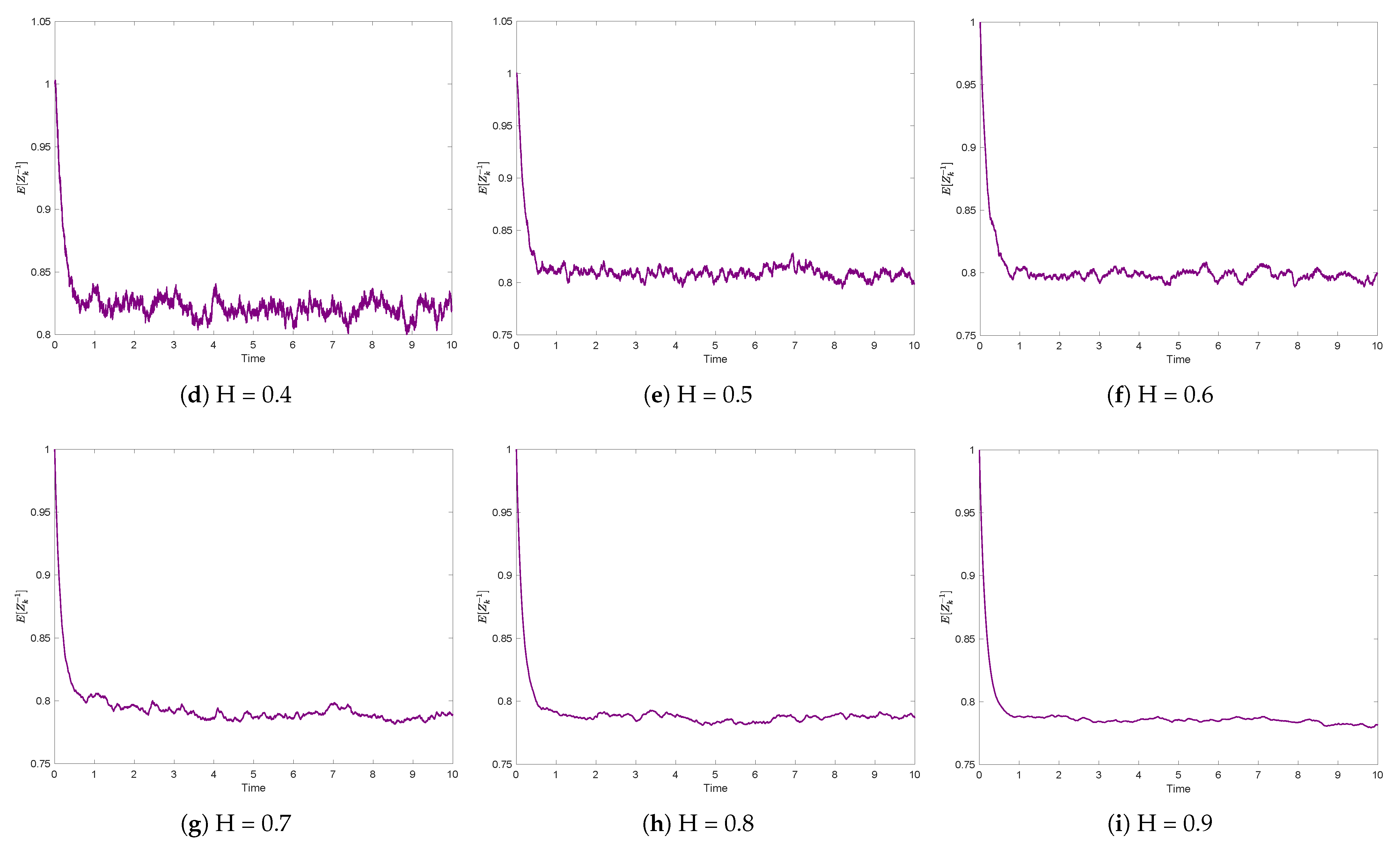
where $\Delta B_{k+1}^H=B_{t_{k+1}}^H-B_{t_k}^H$. Figure 1 displays the behaviors of $\mathbb{E}\left[Z_k\right]$ for Hurst parameters H = 0.1, 0.2, ⋯, 0.9, with $T=10$, $\Delta =2^{-10}$, and the number of paths $M=1000$, while Figure 2 characterizes the corresponding inverse moment $\mathbb{E}\left[Z_k^{-1}\right]$. The expectation is estimated by computing the average of 1000 sample paths.

5.1.1. Strong Convergence

In order to depict the strong convergence rate of the numerical method, we use the numerical solution with $\Delta =2^{-15}$ to represent the exact solution of (16). And the mean square approximation error between the exact solution $Y_{·}$ and the numerical solution $Z_{·}^{{\tau }_l}$ with the level of time discretization ${\tau }_l$ ($l\in \{1,2,3,4\}$) is defined by

$$erro{r}_{\Delta }={\left(\mathbb{E}{\left|Y_T-Z_N^{{\tau }_l}\right|}^2\right)}^{{\displaystyle \frac{1}{2}}}\approx {\left({\displaystyle \frac{1}{1000}}\sum _{i=1}^{1000}{\left|Y_T^i-Z_N^{i,{\tau }_l}\right|}^2\right)}^{{\displaystyle \frac{1}{2}}},$$

(18)

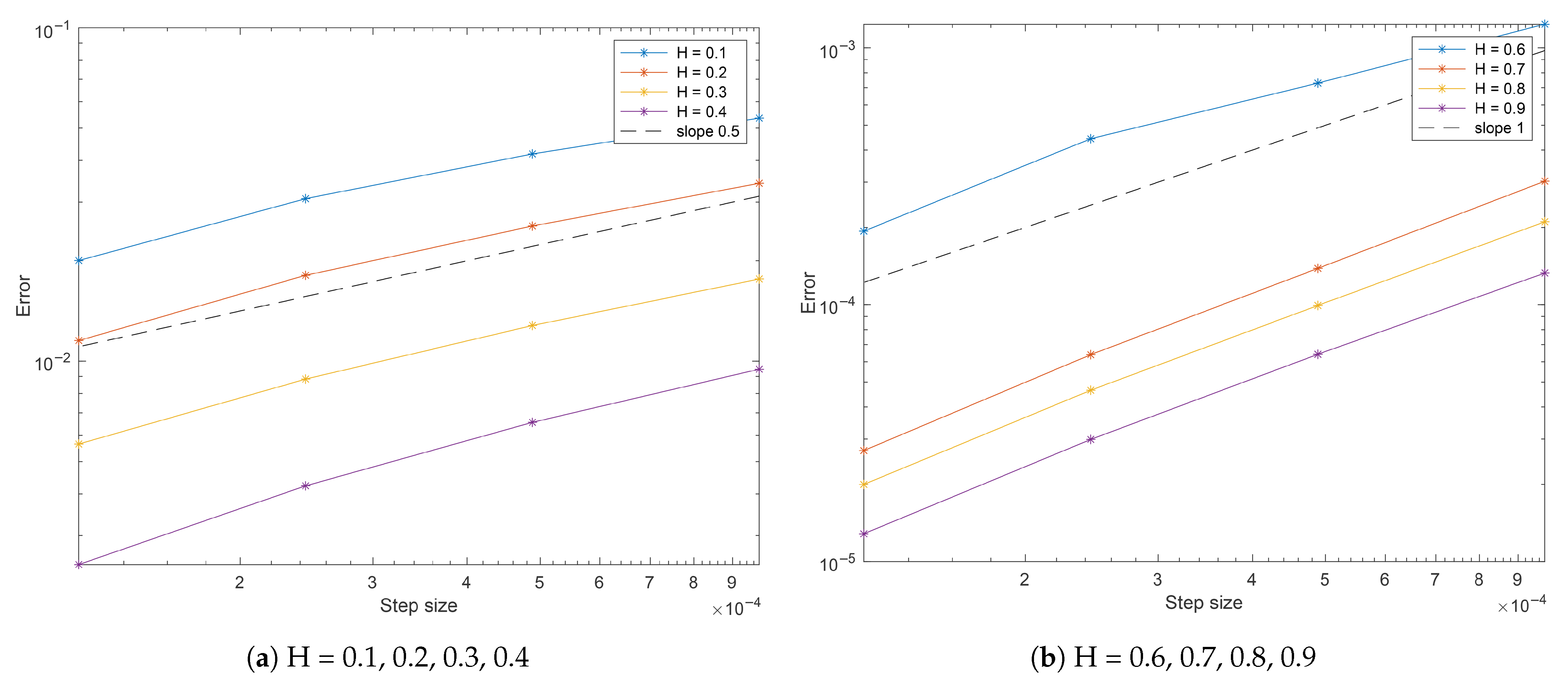
where the discretization level ${\tau }_l$ corresponds to the time step $\Delta$ for $l=1,\dots ,4$, $\Delta \in \{2^{-10},2^{-11},2^{-12},2^{-13}\}$, and i represents the i-$th$ sample path. In Figure 3, we show the mean square approximation error with different Hurst parameters, drawn using MATLAB R2024b, where the strong convergence orders of (16) are presented.

5.1.2. Running Times

The following four tables provide the average times of 30 experiments conducted to obtain the convergence rates of explicit and backward EM methods.

Table 1. Running times in seconds with $H=0.6$ and $T=1$.

	M = 50	M = 100	M = 500	M = 1000
Explicit	1.2713	2.5949	9.8056	18.4476
Backward	2.4108	4.7618	21.0012	43.7890

and

Table 2. Running times in seconds with $H=0.6$ and $T=2$.

	M = 50	M = 100	M = 500	M = 1000
Explicit	1.8593	3.6351	18.1139	35.6824
Backward	4.3168	8.4042	41.0005	80.0627

illustrate the running times of (17) and the backward EM method under different numbers of paths ($M=50,100,500,1000$) for Hurst parameter $H=0.6$ at $T=1$ and $T=2$, respectively.

Table 3. Running times in seconds with $H=0.9$ and $T=1$.

	M = 50	M = 100	M = 500	M = 1000
Explicit	1.2908	2.1439	10.1114	18.3588
Backward	2.4238	4.4650	20.9171	41.4412

and

Table 4. Running times in seconds with $H=0.9$ and $T=2$.

	M = 50	M = 100	M = 500	M = 1000
Explicit	1.9005	3.6695	17.8736	34.7272
Backward	4.3894	8.5113	40.3358	81.1058

present analogous comparisons for $H=0.9$ at $T=1$ and $T=2$, respectively.

5.1.3. Sensitivity Analysis

This subsection conducts a numerical sensitivity analysis of the Hurst parameter H for (16), motivated by the established significance in applications [32,33]. When $H=0.5$, (16) can be written as

$$d{\tilde{Y}}_t=\left(2{\tilde{Y}}_t^{-2}-{\tilde{Y}}_t+2{\tilde{Y}}_t^2-1.5{\tilde{Y}}_t^3\right)dt-d{B}_t,$$

(19)

with the initial value $Y_0=1$, and $B_t$ is the standard Brownian motion. Then, we define the error

$$erro{r}_H={\left(\mathbb{E}{\left|Y_T^H-{\tilde{Y}}_T\right|}^2\right)}^{{\displaystyle \frac{1}{2}}}\approx {\left({\displaystyle \frac{1}{500}}\sum _{i=1}^{500}{\left|Y_T^{i,H}-{\tilde{Y}}_N^i\right|}^2\right)}^{{\displaystyle \frac{1}{2}}},$$

(20)

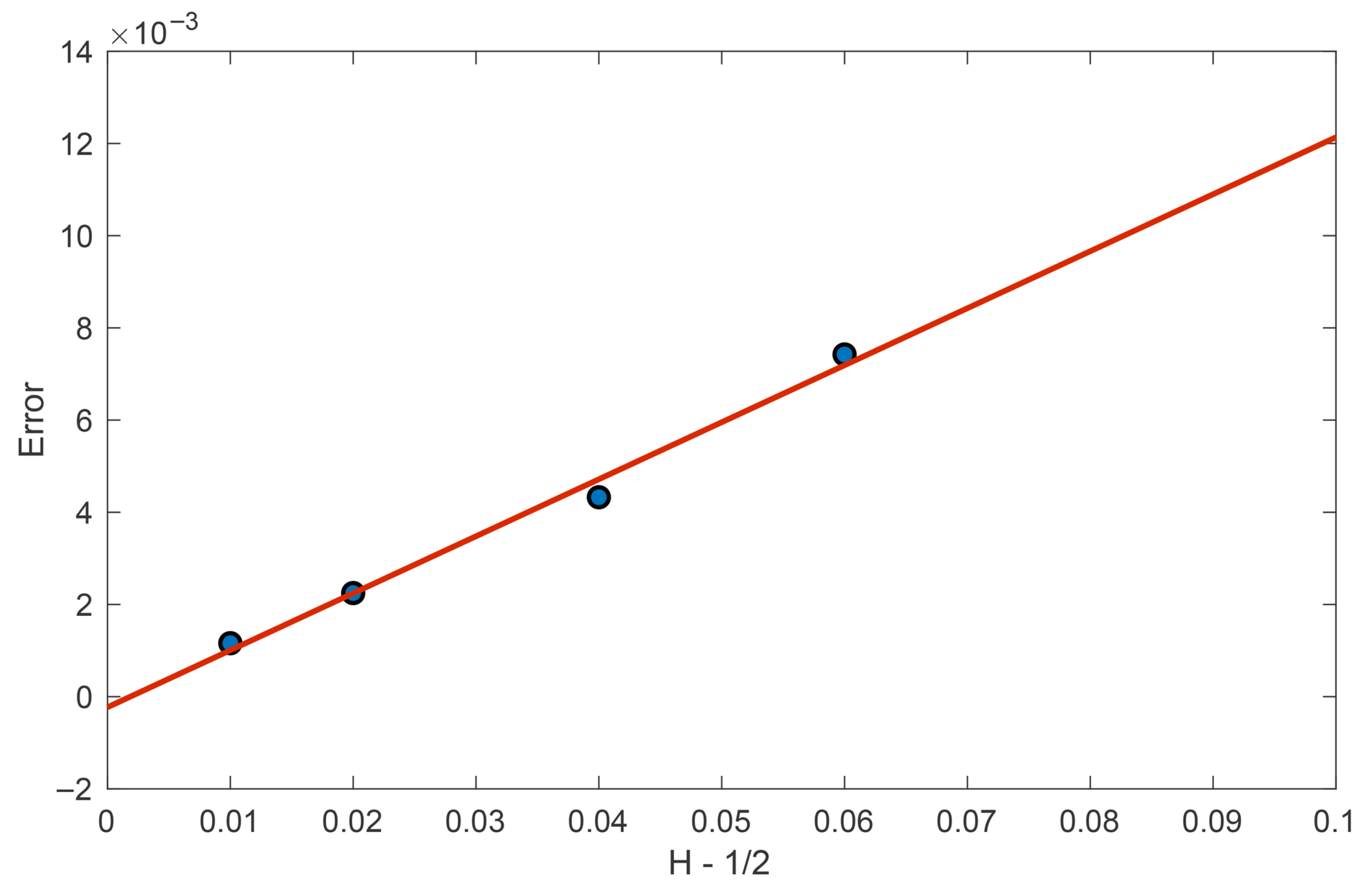
with $T=1$. Here, the subscript H in $Y^H$ and $erro{r}_H$ distinguishes the solution to (16) and its associated error for different Hurst parameters. The numerical solutions with $\Delta =2^{-15}$ are regarded as the exact solutions for (16) and (19). We plot the regression line in Figure 4, which reveals a linear relationship between error (20) and $H-1/2$.

5.2. Example 2

Next, consider the following two-dimensional SDE. Let ${\mathbf{X}}_t={(X_t^1,X_t^2)}^{\top }$ be a two-dimensional stochastic process that satisfies

$$d{\mathbf{X}}_t=\mathbf{A}{\mathbf{X}}_{t}dt+\mathbf{G}d{\mathbf{B}}_t^H,t\in [0,T],$$

(21)

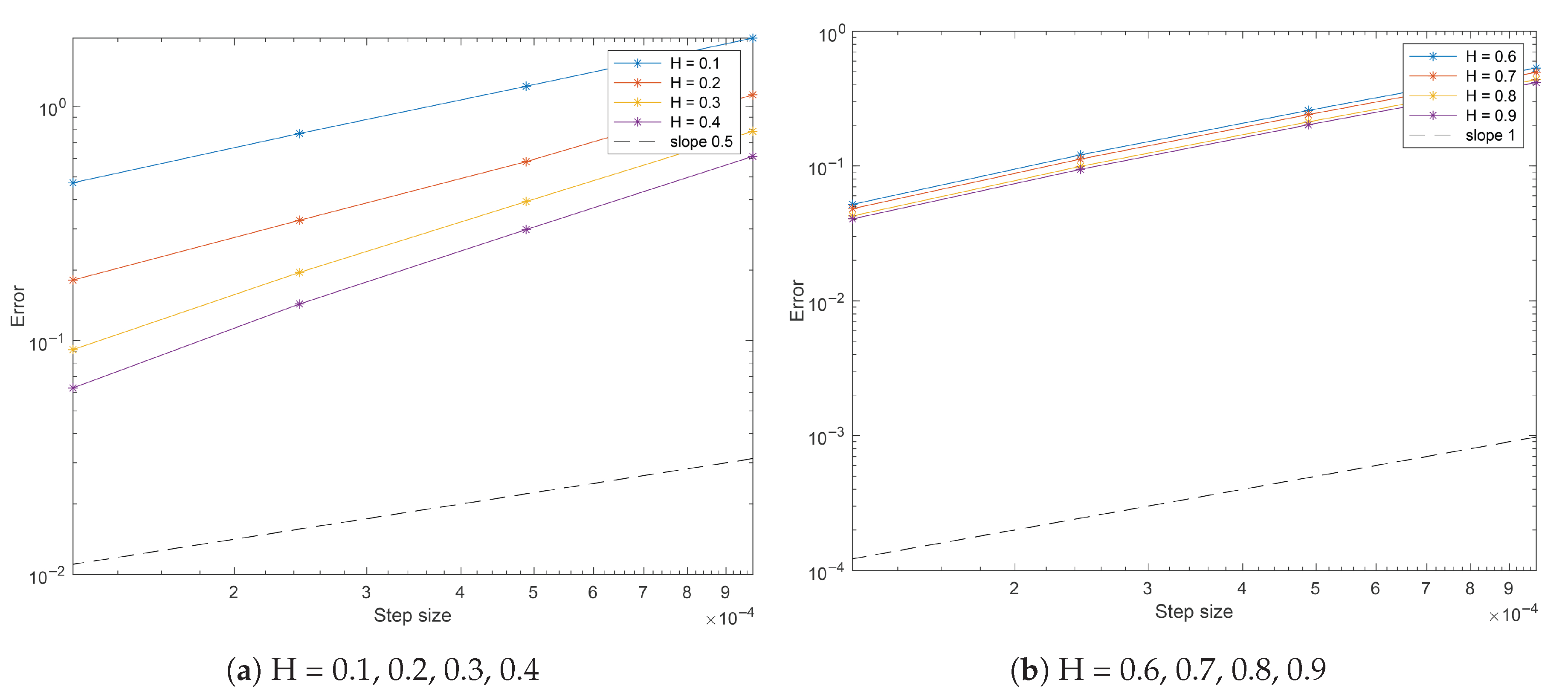
with initial value ${\mathbf{X}}_0={(2,2)}^{\top }$. Here, ${\mathbf{B}}_t^H={(B_t^{1,H},B_t^{2,H})}^{\top }$, with $B_t^{1,H}$ and $B_t^{2,H}$ as two independent one-dimensional FBMs. $\mathbf{A}=\left(\begin{array}{cc}4& 1\\ 1& 4\end{array}\right)$ and $\mathbf{G}=\left(\begin{array}{cc}1& 0\\ 0& 1\end{array}\right)$ are symmetric matrices. The numerical solution approximated by the Euler method with $\Delta =2^{-15}$ is regarded as the exact solution. Figure 5 demonstrates the strong convergence results, computed by (18), between the exact solution and its numerical approximations with $\Delta \in \{2^{-10},2^{-11},2^{-12},2^{-13}\}$.

The theoretical analysis and numerical experiments show that under specific parameter constraints, the explicit positivity-preserving method is effective. However, if these constraints are violated, the explicit positivity-preserving method may fail.

References

1. Aït-Sahalia, Y. Testing continuous-time models of the spot interest rate. Rev. Financ. Stud. 1996, 9, 385–426. [Google Scholar] [CrossRef]
2. Hong, Y.; Lin, H.; Wang, S. Modeling the dynamics of Chinese spot interest rates. J. Bank. Financ. 2010, 34, 1047–1061. [Google Scholar] [CrossRef]
3. Aït-Sahalia, Y. Transition densities for interest rate and other nonlinear diffusions. J. Financ. 1999, 54, 1361–1395. [Google Scholar] [CrossRef]
4. Szpruch, L.; Mao, X.; Higham, D.J.; Pan, J. Numerical simulation of a strongly nonlinear Aït-Sahalia-type interest rate model. BIT Numer. Math. 2011, 51, 405–425. [Google Scholar] [CrossRef]
5. Emmanuel, C.; Mao, X. Truncated EM numerical method for generalised Ait-Sahalia-type interest rate model with delay. J. Comput. Appl. Math. 2021, 383, 113137. [Google Scholar] [CrossRef]
6. Liu, R.; Cao, Y.; Wang, X. Unconditionally positivity-preserving explicit Euler-type schemes for a generalized Aït-Sahalia model. Numer. Algorithms 2025, 98, 651–675. [Google Scholar] [CrossRef]
7. Deng, S.; Fei, C.; Fei, W.; Mao, X. Positivity-preserving truncated Euler–Maruyama method for generalised Ait-Sahalia-type interest model. BIT Numer. Math. 2023, 63, 59. [Google Scholar] [CrossRef]
8. Wang, B.; Zhu, Q. The stabilization problem for a class of discrete-time semi-Markov jump singular systems. Automatica 2025, 171, 111960. [Google Scholar] [CrossRef]
9. Bao, J.; Huang, X. Approximations of McKean–Vlasov Stochastic Differential Equations with Irregular Coefficients. J. Theor. Probab. 2022, 35, 1187–1215. [Google Scholar] [CrossRef]
10. Xie, L.; Zhang, X. Ergodicity of stochastic differential equations with jumps and singular coefficients. Annales de l’Institut Henri Poincaré, Probabilités et Statistiques. Ann. Inst. H. Poincaré Probab. Statist. 2020, 56, 175–229. [Google Scholar] [CrossRef]
11. Merton, R.C. Theory of rational option pricing. Bell J. Econ. 1973, 4, 141–183. [Google Scholar] [CrossRef]
12. Cox, J.C.; Ingersoll, J.E.; Ross, S.A. A theory of the term structure of interest rates. Econometrica 1985, 53, 385–407. [Google Scholar] [CrossRef]
13. Chen, J.; Li, X.; Shao, Y. Numerical analysis of fractional order Black–Scholes option pricing model with band equation method. J. Comput. Appl. Math. 2024, 451, 115998. [Google Scholar] [CrossRef]
14. Biagini, F.; Hu, Y.; Øksendal, B.; Zhang, T. Stochastic Calculus for Fractional Brownian Motion and Applications; Springer: London, UK, 2008. [Google Scholar]
15. Mishura, Y. Stochastic Calculus for Fractional Brownian Motion and Related Processes; Springer: Berlin/Heidelberg, Germany, 2008. [Google Scholar]
16. Rahman, M.; Karaca, Y.; Agarwal, R.P.; David, S.A. Mathematical modelling with computational fractional order for the unfolding dynamics of the communicable diseases. Appl. Math. Sci. Eng. 2024, 32, 2300330. [Google Scholar] [CrossRef]
17. Zhang, S.; Yuan, C. Stochastic differential equations driven by fractional Brownian motion with locally Lipschitz drift and their implicit Euler approximation. Proc. R. Soc. Edinburgh Sect. A 2021, 151, 1278–1304. [Google Scholar] [CrossRef]
18. Hong, J.; Huang, C.; Kamrani, M.; Wang, X. Optimal strong convergence rate of a backward Euler type scheme for the Cox-Ingersoll-Ross model driven by fractional Brownian motion. Stochastic Process. Appl. 2020, 130, 2675–2692. [Google Scholar] [CrossRef]
19. Gao, X.; Wang, J.; Wang, Y.; Yang, H. The truncated Euler-Maruyama method for CIR model driven by fractional Brownian motion. Stat. Probab. Lett. 2022, 189, 109573. [Google Scholar] [CrossRef]
20. Gao, S.; Guo, Q.; Liu, Z.; Yuan, C. Euler–Maruyama scheme for delay-type stochastic McKean–Vlasov equations driven by fractional Brownian motion. Commun. Nonlinear Sci. Numer. Simul. 2025, 149, 108927. [Google Scholar] [CrossRef]
21. Ma, W.; Liu, W.; Zhu, Q.; Shi, K. Dynamics of the Exponential Population Growth System with Mixed Fractional Brownian Motion. Complexity 2021, 2021, 5079147. [Google Scholar] [CrossRef]
22. Zhou, H.; Hu, Y.; Zhao, J. Numerical method for singular drift stochastic differential equation driven by fractional Brownian motion. J. Comput. Appl. Math. 2024, 447, 115902. [Google Scholar] [CrossRef]
23. Naserifar, S.; Mirzaee, F. Innovative computational model for variable order fractional Brownian motion and solving stochastic differential equations. Numer. Algorithms 2025, 1–30. [Google Scholar] [CrossRef]
24. Arthi, G.; Park, J.H.; Jung, H.Y. Existence and exponential stability for neutral stochastic integrodifferential equations with impulses driven by a fractional Brownian motion. Commun. Nonlinear Sci. Numer. Simul. 2016, 32, 145–157. [Google Scholar] [CrossRef]
25. Li, P.; Han, L.; Xu, C.; Peng, X.; Rahman, M.; Shi, S. Dynamical properties of a meminductor chaotic system with fractal–fractional power law operator. Chaos Solitons Fractals 2023, 175, 114040. [Google Scholar] [CrossRef]
26. Qu, H.; Rahman, M.; Arfan, M. Fractional model of smoking with relapse and harmonic mean type incidence rate under Caputo operator. Appl. Math. Comput. 2023, 69, 403–420. [Google Scholar]
27. Chassagneux, J.-F.; Jacquier, A.; Mihaylov, I. An explicit Euler scheme with strong rate of convergence for financial SDEs with non-Lipschitz coefficients. SIAM J. Financ. Math. 2016, 7, 993–1021. [Google Scholar] [CrossRef]
28. Zähle, M. Integration with respect to fractal functions and stochastic calculus I. Probab. Theory Relat. Fields 1998, 111, 333–374. [Google Scholar] [CrossRef]
29. Nualart, D. The Malliavin Calculus and Related Topics, 2nd ed.; Springer: Berlin/Heidelberg, Germany, 2006. [Google Scholar]
30. Alòs, A.; Nualart, D. Stochastic integration with respect to the fractional Brownian motion. Stoch. Stoch. Rep. 2003, 75, 129–152. [Google Scholar] [CrossRef]
31. Zhou, H.; Hu, Y.; Liu, Y. Backward Euler method for stochastic differential equations with non-Lipschitz coefficients driven by fractional Brownian motion. BIT Numer. Math. 2023, 63, 40. [Google Scholar] [CrossRef]
32. Haress, E.M.; Richard, A. Long-time Hurst regularity of fractional stochastic differential equations and their ergodic means. J. Theoret. Probab. 2025, 38, 24. [Google Scholar] [CrossRef]
33. Richard, A.; Talay, D. Lipschitz continuity in the Hurst parameter of functionals of stochastic differential equations driven by a fractional Brownian motion. Electron. J. Probab. 2024, 29, 1–70. [Google Scholar] [CrossRef]
Figure 1. E [ Z k ] for different Hurst parameters: H = 0.1 , 0.2 , 0.3 , 0.4 , 0.5 , 0.6 , 0.7 , 0.8 , 0.9 .
Symmetry 17 01649 g001
Figure 2. E [ Z k 1 ] for different Hurst parameters: H = 0.1 , 0.2 , 0.3 , 0.4 , 0.5 , 0.6 , 0.7 , 0.8 , 0.9 .
Symmetry 17 01649 g002aSymmetry 17 01649 g002b
Figure 3. Convergence rates for Hurst parameters: H = 0.1 , 0.2 , 0.3 , 0.4 , 0.6 , 0.7 , 0.8 , 0.9 .
Symmetry 17 01649 g003
Figure 4. Regression of (20) against H 1 / 2 .
Symmetry 17 01649 g004
Figure 5. Convergence rates for Hurst parameters: H = 0.1 , 0.2 , 0.3 , 0.4 , 0.6 , 0.7 , 0.8 , 0.9 .
Symmetry 17 01649 g005