Article

Statistical Learning-Assisted Evolutionary Algorithm for Digital Twin-Driven Job Shop Scheduling with Discrete Operation Sequence Flexibility

1
School of Management, Xihua University, Chengdu 610039, China
2
School of Mechanical Science and Engineering, Huazhong University of Science and Technology, Wuhan 430074, China
3
School of Computer Science, Liaocheng University, Liaocheng 252000, China
*
Author to whom correspondence should be addressed.
Symmetry 2025, 17(10), 1614; https://doi.org/10.3390/sym17101614
Submission received: 1 September 2025 / Revised: 19 September 2025 / Accepted: 22 September 2025 / Published: 29 September 2025
(This article belongs to the Special Issue Symmetry/Asymmetry in Operations Research)

Abstract

With the rapid development of Industry 5.0, smart manufacturing has become a key focus in production systems. Hence, achieving efficient planning and scheduling on the shop floor is important, especially in job shop environments, which are widely encountered in manufacturing. However, traditional job shop scheduling problems (JSP) assume fixed operation sequences, whereas in modern production, some operations exhibit sequence flexibility, referred to as sequence-free operations. To mitigate this gap, this paper studies the JSP with discrete operation sequence flexibility (JSPDS), aiming to minimize the makespan. To effectively solve the JSPDS, a mixed-integer linear programming model is formulated to solve small-scale instances, verifying multiple optimal solutions. To enhance solution quality for larger instances, a digital twin (DT)–enhanced initialization method is proposed, which captures expert knowledge from a high-fidelity virtual workshop to generate high-quality initial population. In addition, a statistical learning-assisted local search method is developed, employing six tailored search operators and Thompson sampling to adaptively select promising operators during the evolutionary algorithm (EA) process. Extensive experiments demonstrate that the proposed DT-statistical learning EA (DT-SLEA) significantly improves scheduling performance compared with state-of-the-art algorithms, highlighting the effectiveness of integrating digital twin and statistical learning techniques for shop scheduling problems. Specifically, in the Wilcoxon test, pairwise comparisons with the other algorithms show that DT-SLEA has p-values below 0.05. Meanwhile, the proposed framework provides guidance on utilizing symmetry to improve optimization in complex manufacturing systems.

1. Introduction

Under the background of Industry 5.0, moving toward smart manufacturing has become a key point in the overall strategic layout [1]. Industry 5.0 has emerged as an evolution beyond Industry 4.0, focusing not only on digitalization and automation but also on human–machine collaboration, sustainability, and resilience. Unlike Industry 4.0, which primarily emphasized cyber-physical systems, big data, and IoT-driven smart factories, Industry 5.0 highlights the integration of human creativity with advanced technologies such as artificial intelligence, robotics, and digital twins. This paradigm shift aims to create more adaptive, sustainable, and human-centric manufacturing systems that can address both productivity and social value.
Building on this foundation, Industry 5.0 provides a strategic framework for smart manufacturing by promoting flexible, efficient, and energy-aware production systems. It encourages enterprises to pursue not only operational efficiency but also resource optimization and environmental sustainability. Scheduling, logistics coordination, and intelligent decision-making have therefore become critical to realizing these objectives.
In this context, achieving effective planning and scheduling on the shop floor is a major challenge. Many scholars have made efforts in this field, such as job shop scheduling (JSP) [2], flexible job shop scheduling (FJSP) [3], hybrid flow shop scheduling (HFSP) [4], and so on. The JSP problem is a relatively fundamental model in manufacturing, from which many complex production problems have evolved, including assembly scheduling, automated guided vehicles, and distributed production systems. However, most scholars have assumed that the operation routing of a job is fixed, which means all operations are sequence-constrained operations (SCOs). In recent years, as product complexity has increased, some operations within a job exhibit sequence flexibility, meaning they can be processed at any position in the job’s operation routing [5]. Such operations are referred to as sequence-free operations (SFOs). Unfortunately, only a few scholars have found this condition and have only studied it in the context of FJSP [5,6].
To address this limitation, this paper investigates the JSP with discrete operation sequence flexibility (JSPDS), focusing on minimizing the makespan. The practical importance of JSPDS lies in its ability to reflect the increasing demand for flexible and adaptive production systems in modern manufacturing, where operation sequences cannot always be predetermined. Effectively solving JSPDS can help enterprises reduce makespan, improve resource utilization, and enhance production resilience under Industry 5.0 requirements.
Currently, the mainstream solving methods for shop scheduling are evolutionary algorithms (EA), which utilize evolutionary operators to drive the population to evolve and thereby obtain good solutions [7,8]. However, existing EAs still face challenges in efficiently handling the additional complexity introduced by sequence flexibility, which motivates the development of enhanced frameworks. In this paper, an EA is adopted as the main framework to solve the JSPDS. Two technologies are further introduced to enhance the EA framework, namely digital twin (DT) and statistical learning. Specifically, DT is utilized to enhance the initialization, while statistical learning is employed to improve the local search. By integrating these components, the final framework, termed DT-statistical learning EA (DT-SLEA), is formed. The main contributions of this paper are listed as follows:
(1)
A mixed-integer linear programming (MILP) model is formulated to effectively solve small-scale instances. The experimental results demonstrate that the constructed MILP model can verify 6 optimal solutions in the test set.
(2)
A DT-enhanced initialization method is proposed to improve the quality of the initial population. It first constructs the relation between the physical workshop and the virtual workshop. The virtual workshop utilizes a high-fidelity digital twin environment to optimize the production scheme. Then, imitation learning is employed to absorb expert knowledge in the virtual workshop, and knowledge models are generated. Finally, these knowledge models are used to generate a high-quality initial population.
(3)
A statistical learning-assisted local search method is designed to adaptively select promising search operators at different stages of evolution. Six search operators are specifically designed for the JSPDS, and Thompson sampling is used to achieve adaptive selection of promising search operators.
The remainder of this paper is organized as follows. Section 2 presents a review of related work on JSP, sequence flexibility, DT for shop scheduling, and learning-assisted EA. Section 3 details the problem description and the MILP model formulation. Section 4 introduces the overall architecture of DT-SLEA along with the detailed procedures of the enhanced components. In Section 5, experiments are performed, and the results are analyzed. Finally, Section 6 concludes the paper and outlines directions for future research.

2. Literature Review

2.1. JSP and Sequence Flexibility

JSP, as a fundamental problem in the shop scheduling field, has attracted extensive attention from scholars. To the best of our knowledge, the earliest studies on JSP were published in 1959. Wagner [9] and Bowman [10], respectively, formulated linear programming models for JSP. In 1960, Manne [11] developed a model with fewer variables than the previous two models and achieved better performance. However, these exact methods still could not solve large-scale instances. Hence, scholars have adopted approximation methods to address JSP. Davis [12] utilized a genetic algorithm (GA), while Van Laarhoven et al. [13] applied a simulated annealing (SA) algorithm. Subsequently, researchers found that hybrid optimization methods provide a more effective framework than a single algorithm. For example, Gonçalves et al. [14] proposed a hybrid GA with a local search heuristic, and Wang et al. [15] designed a hybrid GA and SA to effectively solve JSP. Park et al. [16] adopted parallel mechanisms to enhance GA. To successfully update the best-known solutions in JSP, scholars recognized the importance of neighborhood structures, which are more promising for improving solution quality. Among the various neighborhood structures for JSP, the most notable are: N1 proposed by Błażewicz et al. [17], N4 by Dell’Amico and Trubian [18], N5 by Nowicki and Smutnicki [19], N6 by Balas and Vazacopoulos [20], N7 by Zhang et al. [21] and N8 by Xie et al. [22,23]. Afterwards, researchers gradually extended JSP from single-objective to multi-objective problems, considering energy consumption [24,25], total tardiness [26,27], and evolving JSP into more complex problems such as integrated assembly scheduling [28,29], automated guided vehicles [30,31,32], and distributed production systems [33,34].
In recent years, sequence flexibility in job processing routes has inspired many scholars due to its practical value in manufacturing. Alvarez et al. [35] studied FJSP with sequence flexibility in a glass factory. Later, Birgin et al. [36] first formulated a MILP model and proposed benchmark instances for fair comparison. Since then, many researchers have investigated various types of sequence flexibility based on practical applications in industry, such as simultaneous processing of SFOs [37,38,39,40], two or more operations to be processed together [7], different job priorities [41,42,43,44], and discrete operation sequence flexibility [5,6]. Due to the significant application of discrete operation sequence flexibility in manufacturing, this paper focuses on this type.

2.2. DT for Shop Scheduling

DT is an emerging technology in industry, medicine, and defense. It constructs a virtual environment by modeling the physical environment, and then enables real-time monitoring, simulation, prediction, and optimization of system performance. By integrating data from physical entities and updating the virtual counterpart continuously, DT provides valuable insights for decision-making, fault diagnosis, and efficiency improvement [45,46]. Next, recent successful applications of DT in shop scheduling are reviewed.
In recent years, some scholars have integrated DT with deep reinforcement learning (DRL) and EA to solve shop scheduling problems. Regarding DRL, Yan et al. [47] adopted a double-layer Q-learning algorithm to solve FJSP with preventive maintenance, where DT was utilized to construct the problem environment. Geng et al. [48] designed a multi-agent DRL method to address discrete manufacturing workshops with transportation resources under a DT environment. Gao et al. [49] proposed a time-space network-based zero-one programming approach to effectively solve FJSP with conflict-free routing. To achieve real-time interaction between the scheduling system and the physical workshop, they formulated a cloud–edge collaborative DT environment. For EA, Fang et al. [1] designed a DT model to enable real-time and precise scheduling in dynamic JSP and developed an improved NSGA-II algorithm. Chen et al. [50] constructed a DT scheduling model combined with physical entities and proposed a hybrid particle swarm optimization algorithm to solve multi-objective FJSP. Gao et al. [51] formulated a DT environment for real-time monitoring and developed an improved multi-objective EA. In addition, Zhang et al. [52] designed a DT framework to efficiently detect disturbances and trigger timely rescheduling in dynamic JSP.
In summary, DT can serve as a bridge between the physical shop floor and the virtual shop floor, and the formulated DT model can achieve real-time updates by absorbing new production data. However, most scholars have applied the DT model mainly as a test platform to verify the performance of proposed algorithms. As a result, expert knowledge embedded in the DT model has been underutilized. To mitigate this gap, this paper incorporates DT expert knowledge into the problem to enhance initialization, thereby improving the quality of the initial population.

2.3. Learning-Assisted EA

To improve the performance of EA in shop scheduling problems, scholars have investigated learning-assisted EA. The most common approaches include reinforcement learning-assisted, feedback learning-assisted, meta-reinforcement learning-assisted, and imitation learning-assisted algorithms. Each of these methods has its own advantages and has demonstrated good performance on various types of problems.
Considering reinforcement learning-assisted approaches, Pan et al. [53] designed a reinforcement learning (RL)-based mating selection strategy to improve the EA evolution process for solving FJSP with transportation resources. Ma et al. [54] employed DRL to adaptively tune the key parameters of GA in solving FJSP. Similarly, Ding et al. [55] adopted the PPO algorithm to dynamically adjust the control parameters of EA for solving FJSP with multiplicity. Chang et al. [8] utilized Q-learning-driven variable neighborhood search (VNS) to enhance a memetic algorithm for multi-objective FJSP. For feedback learning-assisted approaches, Wang et al. [56] employed historical information from a feedback learning model to adaptively select search operators in a cooperative memetic algorithm for solving energy-aware distributed flow-shops with flexible assembly scheduling. Furthermore, Wang et al. [57] proposed a feedback learning-based memetic algorithm, in which success and failure tables were used to record the performance of search operators, and this information was leveraged for adaptive operator selection. Considering meta-reinforcement learning-assisted approaches, Zhang et al. [4] developed a meta learning-driven VNS algorithm to solve HFSP with learning and forgetting effects. Shao et al. [58] adopted meta-Q-learning to guide the selection of search operators in EA, effectively solving the energy-efficient distributed fuzzy hybrid blocking flow-shop scheduling problem. For imitation learning-assisted approaches, Cheng et al. [59] applied imitation learning to dynamically select search operators for elite individuals.
In summary, learning mechanisms mainly assist EA in adaptive operator selection and have shown superior performance. However, whether reinforcement learning-assisted, feedback learning-assisted, meta-reinforcement learning-assisted, or imitation learning-assisted, these methods typically introduce a number of additional parameters into EA. This makes parameter setting difficult, and the algorithm performance heavily depends on parameter configuration, which reduces generalizability. To mitigate this gap, this paper adopts statistical learning, specifically Thompson sampling, to adaptively select search operators. This approach does not introduce extra parameters into EA and therefore significantly improves its generalizability.

2.4. Summary

In summary, existing studies on JSP and sequence flexibility reveal that researchers have made significant progress in extending the classical problem to more practical and complex scenarios. Additionally, DT has been increasingly adopted to enable real-time monitoring and interaction between physical and virtual environments, although most studies have used it mainly as a test platform without fully exploiting embedded expert knowledge. Meanwhile, learning-assisted evolutionary algorithms have demonstrated strong potential in adaptive operator selection, but their reliance on additional parameters limits their generalizability. To address these gaps, this paper integrates DT expert knowledge into initialization and employs statistical learning for adaptive operator selection, aiming to enhance both solution quality and algorithm robustness in JSPDS.

3. Problem Description

3.1. JSPDS Definition

The description of the JSPDS problem is as follows: there are n jobs and m machines on the shop floor, and each job’s operations are divided into SCOs and SFOs. Each operation is processed on a specific machine. The SCOs must be processed in a fixed linear sequence, while the SFOs can be processed at any position in the process sequence. Additionally, the JSP sometimes exhibits symmetry, as multiple equivalent schedules may result from interchangeable operation orders that do not affect the makespan, thereby increasing the search complexity.
To further illustrate the JSPDS problem, an example is provided in Figure 1. In this example, there are three jobs and three machines. For Job 1, the SCOs are O11, O12, and the SFOs are O1a, O1b. According to the above description, O12 must be processed after O11 is completed, whereas O1a and O1b can be scheduled at any position in the sequence. For Job 2, the SCOs are O21, O22, and the SFO is O2a. For Job 3, the SCOs are O31, O32, and the SFO is O3a.
As shown in Figure 1, the processing sequence of Job 1 is O11, O1b, O12, O1a; for Job 2, the sequence is O21, O22 and O2a; and for Job 3, the sequence is O3a, O31, and O32. The scheduling result is 51.

3.2. Notations

The parameters and decision variables of the MILP model are provided in Table 1.

3.3. MILP Model

The MILP model is formulated with the objective function (1) and constraints (2)–(8).
min   f = C max
C i , j + p t i , j , k C max , i I , j J i , k K i , j
C i , j + p t i , j , k M * ( 1 B i , j , j ) C i , j , i I , j J i , j J i , k K i , j
B i , j , j + 1 = 1 , i I , j 1 , 2 , , n i S C O 1
B i , j , j + B i , j , j = 1 , i I , j J i , j J i , j < j
C i , j + p t i , j , k C i , j + M ( 1 A i , j , i , j ) , i I , i I , i < i , j J i , j J i , k K i , j K i , j
C i , j + M * A i , j , i , j C i , j + p t i , j , k , i I , i I , i < i , j J i , j J i , k K i , j K i , j
C i , j 0 , i I , j J i
The Formulation (1) specifies the objective of minimizing the makespan, and constraint (2) defines the makespan. Constraint set (3) enforces the processing order of operations within each job. Constraint set (4) ensures that SCOs are processed in a fixed linear sequence, and constraint set (5) regulates the sequencing of SFOs. Constraint sets (6)–(7) impose the machine non-overlap constraints, ensuring that operations assigned to the same machine do not overlap. Constraint (8) enforces nonnegativity of operation start times (i.e., start times are ≥0).

4. DT-SLEA

4.1. DT-SLEA Framework

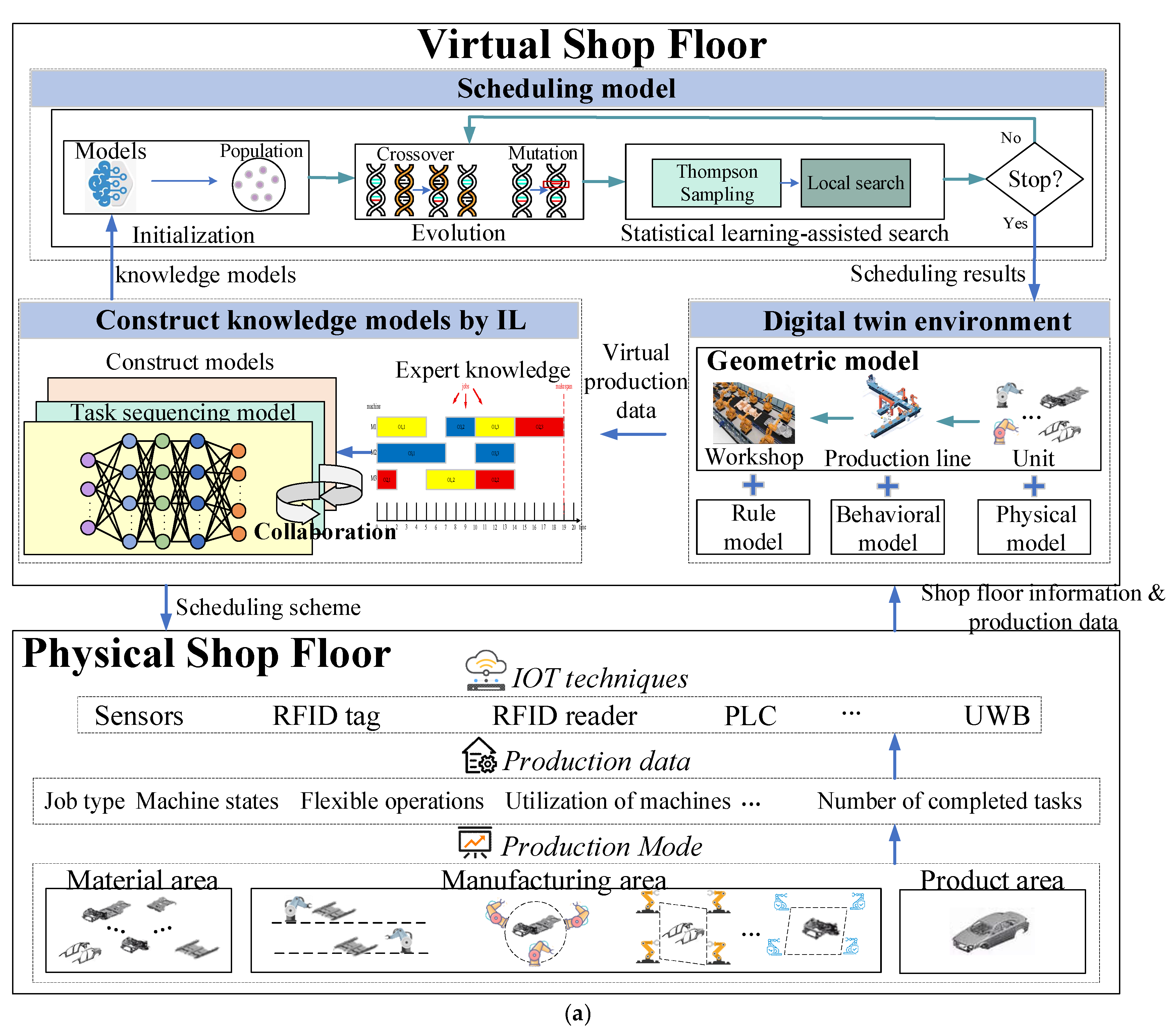
To effectively solve the JSPDS, EA is adopted as the main framework, introducing DT to enhance initialization and using statistical learning to assist local search, thereby forming the DT-SLEA framework. In particular, the framework also considers the symmetry inherent in JSPDS, where multiple equivalent schedules may arise from interchangeable positions of sequence-free operations, and incorporates tailored strategies to improve search efficiency. The visualization of the DT-SLEA framework is shown in Figure 2a.
The analysis begins with the physical shop floor, which consists of the production mode, production data that record the workshop status, and IoT techniques for data transfer to the virtual workshop. After clarifying the structure of the physical shop floor, the virtual shop floor is constructed to solve the JSPDS. The physical and virtual shop floors are connected through the DT environment. Shop floor information and production data are transferred via IoT techniques, and a geometric model is created using modeling software. The virtual workshop layout is reconstructed using CAD data from the physical shop floor, including precise machine positions, workstations, and storage locations, ensuring spatial consistency between the physical and virtual environments. Based on this geometric model, detailed features and constraints are added to formulate the physical model. The physical model contains both static attributes (e.g., names, IDs) and dynamic attributes (e.g., states, processing times). The behavior model is introduced to describe dynamic shop floor behaviors, such as changes in machine operations. This allows the virtual environment to reflect realistic scheduling dynamics. The rule model incorporates production scheduling rules, which allocate waiting jobs to machines. Scheduling constraints such as operation precedence, job priorities, and allocation of waiting jobs to machines are implemented as logical rules, ensuring that the DT accurately represents the physical workshop rules. By combining the geometric model, physical model, behavior model, and rule model, the DT environment is established, ensuring a high degree of consistency between the virtual and physical shop floors.
The construction of knowledge models and scheduling models forms the core of the DT-SLEA framework. Scheduling results generated by these core models are absorbed by the DT environment. As the system operates continuously, the DT model learns from the scheduling results to accumulate expert knowledge. Consequently, the virtual shop floor achieves self-evolution, while the scheduling scheme is fed back to the physical shop floor to guide actual production.
The flow chart of DT-SLEA framework is given in Figure 2b and the core steps of the DT-SLEA framework are as follows:
Step 1: DT-enhanced initialization. From the virtual production data in the DT environment, expert knowledge is extracted. Imitation learning (IL) is then applied to behavior-clone this expert knowledge and construct the knowledge model, i.e., the operation sequencing model. This knowledge model is used to initialize a high-quality population of size Np.
Step 2: Evolution. Based on the crossover probability Pc and mutation probability Pm, crossover and mutation operators are applied to each individual in the population, driving the evolutionary process.
Step 3: Statistical learning-assisted search.
Step 3.1: Thompson sampling. For the six search operators, Thompson sampling is applied to generate their respective selection probabilities.
Step 3.2: Local search. Select Ne elite individuals from the population. For each elite individual, select a search operator according to the probability distribution and apply it.
Step 4: Termination check. If the algorithm runtime reaches the predefined limit, the algorithm stops and outputs the scheduling results to the DT environment. Otherwise, return to Step 2.

4.2. DT-Enhanced Initialization

The core idea of DT-enhanced initialization is to use IL to behavior-clone expert knowledge from the DT model in order to construct the knowledge model. Specifically, the expert knowledge refers to high-quality scheduling schemes represented as OS vectors, while the knowledge model is implemented as a deep neural network with four linear layers. The input dimension corresponds to the length of the OS vector, and the output dimension is the number of operations. The hidden layers have sizes of 256, 128, and 64, respectively.
The process of training the knowledge model with expert knowledge is as follows. The network takes all expert knowledge (operation sequence vectors of equal length) as input and generates action probabilities, each corresponding to a candidate operation. Cross-entropy loss is calculated between the predicted action probabilities and the expert actions (i.e., the operations selected in the expert knowledge) to update the network. The training dataset consists of 100 job shop instances generated from small- and large-scale configurations, with 80% used for training and 20% for validation. Overfitting is prevented using early stopping (if validation loss does not improve for 5 consecutive epochs) and L2 regularization. The network is trained for 20 epochs using the Adam optimizer with a learning rate of 1 × 10⁻⁴. Validation metrics include the mean squared error for predicted operation priorities and accuracy in reproducing high-quality initial sequences. After training, the model is saved and constitutes the knowledge model, which is then used to guide the initialization of the evolutionary algorithm population.
The knowledge model absorbs the expert knowledge and is capable of generating high-quality individuals, thus forming a superior initial population. The generation of individuals proceeds as follows:
First, a job is randomly selected as the starting operation. Then, the knowledge model is used to select the next operation based on the operation probability distribution. This process is repeated iteratively, with the model continuously updating the decision sequence, until a complete operation sequence is constructed.

4.3. Encoding and Decoding

The JSPDS consists solely of the operation sequencing (OS) problem; hence the encoding scheme uses a single-layer vector called the OS vector. An example of this encoding is shown in Figure 3. For SCOs, each integer represents corresponding job operation, and the number of repeated occurrences indicate the operation index for the job. For SFOs, each integer equals the total number of jobs plus the sequential index of the flexible operation. Decoding proceeds step by step: for each integer in the OS vector, select the corresponding operation and process it on the machine until the OS vector is fully traversed.

4.4. Crossover and Mutation

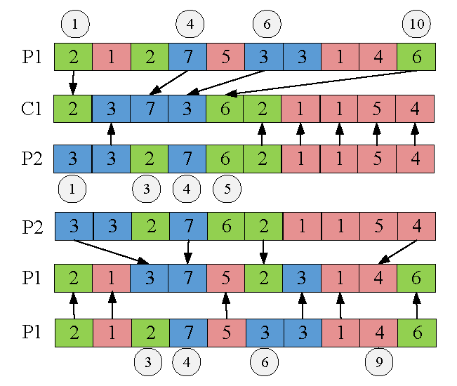
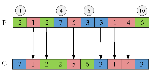
In this study, the crossover and mutation operators employed are the order-based crossover (OBX) and the heterotopic mutation method (HMM) [5]. Illustrative examples are provided in Figure 4 and Figure 5, and their procedures are outlined below.
The detailed steps of OBX:
Step 1: Let l = ⌈length/3⌉. Randomly choose l positions in parent P1. For instance, l = 4, the chosen indices are 1, 4, 6, and 10.
Step 2: Extract the genes of P1 at these indices and denote them as S1. Locate the same elements in parent P2 and record their indices (e.g., 1, 3, 4, and 5). Copy the remaining elements of P2 to offspring C1, then place the genes in S1 back into the recorded positions in the original order.
Step 3: Exchange the roles of P1 and P2 and repeat the procedure to generate offspring C2.
The detailed steps of HMM:
Step 1: Define l = ⌈length/3⌉. Randomly pick l indices from parent P. For example, l = 4, the indices are 1, 4, 6, and 10.
Step 2: Collect the corresponding genes from P, denoted as S1 = [2, 7, 3, 6], and randomly shuffle them to produce a new sequence S2 = [7, 2, 6, 3].
Step 3: Copy the other genes from P into the same positions of offspring C, and then insert the shuffled sequence S2 into the vacant slots sequentially.

4.5. Statistical Learning-Assisted Search

4.5.1. Search Operators

In this paper, six search operators are designed, which are categorized into low-intensity (N1N3) and high-intensity (N4N6) operators, with the latter focusing on critical operations. Their descriptions are as follows:
N1: Randomly select two different operations and exchange them.
N2: Randomly select one operation and insert it before another randomly chosen operation.
N3: Randomly select two different operations and reverse the entire subsequence between them.
N4: Randomly select two different critical operations and exchange them.
N5: Randomly select one critical operation and insert it before another randomly chosen operation.
N6: Randomly select two different critical operations and reverse the entire subsequence between them.

4.5.2. Thompson Sampling and Local Search

The core part of the statistical learning-assisted local search is shown in Algorithm 1. It combines Thompson sampling with local search. The input consists of the search operator set SO = {N1, N2, …, N6} and Ne elite individuals. Lines 1–3 are used to initialize the prior parameters αi and βi for each search operator, where αi and βi are initialized to 1, representing an uninformative prior (i.e., no bias about the operator’s success probability). Lines 4–17 perform local search for each elite individual. The search operator is selected based on Thompson sampling, which samples from the Beta distribution and chooses the operator with the highest sampled performance. If the selected operator improves the solution, the success counter αi is incremented by 1; otherwise, the failure counter βi is incremented by 1. This update gradually reflects the operator’s true performance and influences its selection probability in future iterations. Additionally, if the individual is not improved, the original solution is retained.
Algorithm 1. Thompson sampling and local search
Input: Search operators set SO = {N1, N2, …, N6}, Ne elite individuals
Output: Improved elite individuals
Begin
1: For each search operator Ni ∊ SO do
2:    set αi = 1, βi = 1
3: End for
4: For l = 1 to Ne do
5:    For each search operator Ni ∊ SO
6:      Sample pi∼Beta (αi, βi)
7:      Record pi for search operator Ni
8:    End for
9:    N* = arg max pi
10: Apply the search operator N* to individual l
11: If the operator improves the solution (success) then
12:    α* = α* + 1
13: Else (failure)
14:    b* = b* + 1
15:    Save the original individual
16: End if
17: End for
18: Return Improved elite individuals
End

5. Experiment Results

To evaluate the performance of the proposed MILP model and DT-SLEA, a series of comparative experiments are carried out. The MILP model and DT-SLEA are both implemented in C++ 11 and executed on a computer equipped with an Intel Core i7-12700 CPU and 16 GB of RAM (Kingston Technology), while the MILP model is solved using CPLEX 12.7.1. The time limit for the MILP model is set to 3600 s, whereas DT-SLEA and the other compared algorithms are assigned 5 × m × n × max (ni)/60 s.

5.1. Experimental Instances and Performance Metrics

The experimental instances are generated by us, namely JSPDS01–20, for a total of 20 instances. These include cases with 10 jobs and 10 machines, 20 jobs and 15 machines, 30 jobs and 15 machines, 30 jobs and 20 machines, 40 jobs and 20 machines, 50 jobs and 15 machines, and 50 jobs and 20 machines. Additionally, four real-world production cases are collected from actual factories to further validate the effectiveness and practicality of the proposed framework. All instances can be downloaded from https://github.com/sdadaawa/JSPDS (accessed on 23 September 2025). The performance metric used is the relative percentage increase (RPI). The calculation of the RPI is as follows:
R P I = C max i C max b e s t C max b e s t × 100 %
where Cmaxi is the makespan obtained by algorithm i, and Cmaxbest is the minimal makespan among all comparison algorithms.

5.2. MILP Model Validation

In this section, the MILP model is evaluated. Table 2 presents the experimental results of the MILP model. The term Cmax denotes the result achieved by the MILP model in these instances, and the term Time refers to the solving time of the instance. The unit for time is minutes. As shown in Table 2, the MILP model verifies the optimal solutions for JSPDS 01–06, a total of six instances. For JSPDS 07–20, the MILP model cannot guarantee optimality but is able to obtain feasible solutions.
In summary, the MILP model can effectively solve small-scale instances, but for large-scale instances, it may fail to produce high-quality solutions. To address these challenges, we propose DT-SLEA, and the results are presented in the following section.

5.3. Parameter Settings

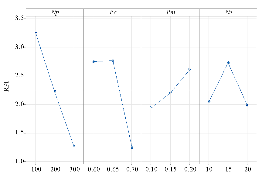
The parameters of DT-SLEA are population size Np, crossover probability Pc, mutation probability Pm, and the number of elite individuals to perform local search Ne. Taguchi analysis is adopted to identify the most suitable parameter combination. The factor levels for these parameters are as follows: Np = {100, 200, 300}, Pc = {0.60, 0.65, 0.70}, Pm = {0.10, 0.15, 0.20}, and Ne = {10, 15, 20}. The experiments are performed on JSPDS20, and each parameter configuration is executed 10 times. The main effects plot of the parameter configurations is shown in Figure 6. Based on Figure 6, the best parameters are set as follows: Np = 300, Pc = 0.70, Pm = 0.10, and E = 20. Specifically, the parameters are set to these values because they yield the minimal RPI, which corresponds to the objective of our study.

5.4. Effectiveness of All Improved Components

In this section, the effectiveness of all improved components is evaluated. Four variant algorithms are considered: EA refers to DT-SLEA without DT-enhanced initialization and statistical learning-assisted local search, DT-EA refers to DT-SLEA without statistical learning-assisted local search, and SLEA refers to DT-SLEA without DT-enhanced initialization. Additionally, to evaluate the effectiveness of statistical learning, another adaptive selection mechanism is applied to the EA for comparison, namely the ε-greedy EA. It uses the epsilon-greedy strategy to adaptively select operations during the evolutionary process. The comparison results of EA, DT-EA, SLEA, ε-greedy EA, and DT-SLEA are presented in Table 3. “Best” and “Ave” denote the best RPI from 10 runs and the average RPI over 10 runs, respectively.
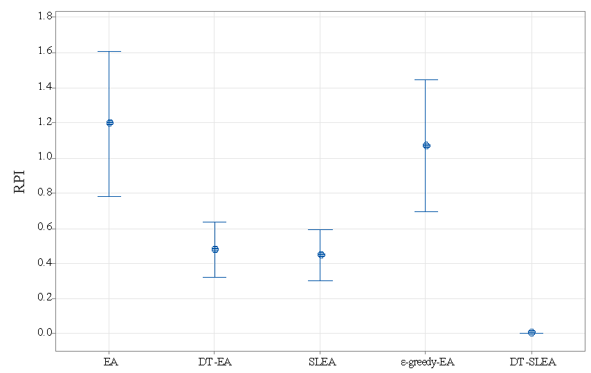
As shown in Table 3, DT-SLEA achieves the best RPI values in both Best and Ave. For the small-scale instances JSPDS01–06, the variant algorithms also reach optimal results. For the large-scale instances, their performance is inferior to that of DT-SLEA. To intuitively illustrate the performance differences between DT-SLEA and the other variant algorithms, the interval plot is shown in Figure 7. As depicted in Figure 7, EA performs the worst, DT-SLEA performs the best, and DT-EA, SLEA and ε-greedy EA perform worse than DT-SLEA but better than EA. However, SLEA performs better than the ε-greedy EA, reflecting that statistical learning is more effective than the epsilon-greedy strategy. The reason is that the epsilon-greedy strategy does not utilize statistical information from the evolutionary process and only relies on the parameter ε to control operation selection. All the above experiments demonstrate the effectiveness of the improved components.
Table 4 presents the results of the Wilcoxon test. DT-SLEA is compared with EA, DT-EA, SLEA and ε-greedy EA, and the p-values for all comparisons are less than 0.05, indicating that DT-SLEA is statistically superior to the other algorithms.
In summary, the DT-enhanced initialization and statistical learning-assisted local search effectively improve the performance of EA. By integrating expert knowledge from the DT model and statistical data from the local search process, the EA obtains a high-quality initial population and adaptively selects promising search operators.

5.5. Comparison of DT-SLEA with Other Algorithms

In this section, DT-SLEA is compared with existing state-of-the-art algorithms for job shop scheduling, namely SMA [60], CC-GP-HH [2], and KLCACO [61]. Additionally, the DRL-based algorithm has been compared to further demonstrate the performance of DT-SLEA, namely DRL-Wang [62] and DRL-Zhang [63].
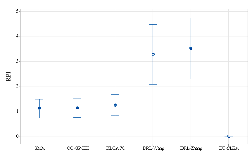
From Table 5, it can be observed that DT-SLEA consistently delivers the best RPI results in terms of both the Best and Ave metrics. For small-scale instances (JSPDS01–06), all algorithms are able to obtain optimal solutions. However, when tackling large-scale instances, the comparison approaches show weaker performance compared with DT-SLEA. To provide a clearer comparison, Figure 8 presents the interval plot. As illustrated, DT-SLEA outperforms the others, while SMA, CC-GP-HH, SLEA, DRL-Wang and DRL-Zhang perform less effectively. Among these five, the overall results are relatively close; nevertheless, SMA demonstrates the best performance, CC-GP-HH and SLEA follow closely, DRL-Wang and DRL-Zhang lag behind.
The statistical significance of these differences is confirmed by the Wilcoxon test results shown in Table 6. Across all pairwise comparisons between DT-SLEA and the other algorithms, the p-values are below 0.05, which verifies that DT-SLEA is statistically superior.
In summary, the effectiveness of DT-SLEA is verified. Its performance on the test set surpasses that of state-of-the-art algorithms. The success of DT-SLEA mainly stems from two aspects: (1) the DT-enhanced initialization ensures a high-quality initial population by leveraging digital twin simulation and imitation learning, and (2) the statistical learning-assisted local search adaptively selects suitable search operators, thereby improving search efficiency.

5.6. Case Study

In this section, four real-world production cases are introduced to further evaluate the practicality and effectiveness of the proposed DT-SLEA framework. These cases are provided by actual workshops with different scales and characteristics, covering diverse machine layouts, job types, and processing times. In Case 1, there are 10 jobs and 10 machines; in Case 2, there are 30 jobs and 20 machines. In Cases 3 and 4, there are 50 jobs and 20 machines. By applying DT-SLEA to these real-world scenarios, the framework’s ability to handle practical scheduling challenges is examined. The results are compared with conventional scheduling strategies and existing state-of-the-art algorithms to demonstrate the adaptability and robustness of DT-SLEA in realistic manufacturing environments. Specifically, the conventional scheduling strategies are first-in-first-out (FIFO), least remaining processing time (LWKR) and most remaining processing time (MWKR). The internal operation sequencing of each job is randomly determined at the beginning, and each rule is executed 10 times.
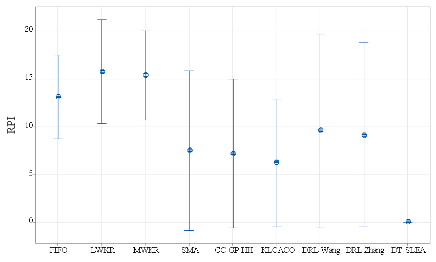
The experimental results are summarized in Table 7. It can be observed that DT-SLEA consistently outperforms conventional scheduling strategies and state-of-the-art algorithms across all four cases. In particular, DT-SLEA achieves lower RPI metrics, reflecting its efficiency in solution quality. Due to the absence of an optimization process and relying solely on manual design, the conventional scheduling strategies show the worst performance. Although in Case 1, where the production scale is limited, DT-SLEA does not show a clear advantage over the existing state-of-the-art algorithms. However, in Cases 2–4, where the job numbers and machine configurations are more complex, DT-SLEA demonstrates a more significant advantage. Figure 9 presents the interval plot for DT-SLEA, conventional scheduling strategies and state-of-the-art algorithms.
Overall, the results in Table 7 verify that DT-SLEA is not only effective in our randomly generated instances but also practical and robust when applied to real-world production scenarios.

6. Conclusions and Future Research

In this paper, the JSPDS problem is studied, which allows certain operations to be processed at any position in a job’s operation routing. A MILP model was formulated to solve small-scale instances, verifying multiple optimal solutions. To address larger instances, a DT-enhanced initialization method was proposed to generate high-quality initial populations by capturing expert knowledge from a high-fidelity virtual workshop. Furthermore, a statistical learning-assisted local search method was developed, employing six tailored search operators and Thompson sampling to adaptively select promising operators within an EA framework. Extensive experiments demonstrate that the proposed DT-SLEA outperforms state-of-the-art algorithms in terms of makespan minimization, while effectively addressing the symmetry inherent in JSPDS, where sequence-free operations may have interchangeable positions leading to equivalent schedules and highlighting the effectiveness of integrating digital twin and statistical learning techniques for complex shop scheduling problems.
Despite the promising results, the present work has certain limitations. The MILP model is restricted to small-scale instances due to computational complexity, and the proposed DT–SLEA mainly addresses single-objective scheduling under deterministic environments [64]. For future research, several directions are suggested. First, the proposed framework can be extended to multi-objective scheduling scenarios, such as optimizing both makespan and energy consumption. Second, incorporating dynamic production environments with uncertain processing times or machine breakdowns could further enhance the robustness of the approach. Finally, exploring more advanced machine learning methods to guide the search operators or to predict high-quality initial solutions may further improve computational efficiency and solution quality [65,66].

Author Contributions

Conceptualization, Y.J., W.C., L.M. and C.Z.; methodology, Y.J., W.C., L.M. and C.Z.; software, W.C. and L.M.; validation, W.C., L.M. and C.Z.; formal analysis, Y.J., W.C., L.M. and C.Z.; investigation, Y.J., W.C., L.M. and C.Z.; resources, W.C., L.M. and C.Z.; data curation, W.C., L.M. and C.Z.; writing—original draft preparation, Y.J., W.C., L.M. and C.Z.; writing—review and editing, Y.J., W.C., L.M. and C.Z.; visualization, Y.J., W.C., L.M. and C.Z.; supervision, L.M. and C.Z.; project administration, Y.J., L.M. and C.Z.; funding acquisition, C.Z. All authors have read and agreed to the published version of the manuscript.

Funding

This research was funded by the National Science and Technology Major Project, grant number 2024ZD0707501.

Data Availability Statement

The original contributions proposed in the study are included in this paper, and further inquiries can be directly addressed to the corresponding author.

Conflicts of Interest

The authors declare no conflicts of interest.

References

  1. Fang, Y.; Peng, C.; Lou, P.; Zhou, Z.; Hu, J.; Yan, J. Digital-twin-based job shop scheduling toward smart manufacturing. IEEE Trans. Ind. Inform. 2019, 15, 6425–6435. [Google Scholar] [CrossRef]
  2. Zeiträg, Y.; Rui Figueira, J.; Figueira, G. A cooperative coevolutionary hyper-heuristic approach to solve lot-sizing and job shop scheduling problems using genetic programming. Int. J. Prod. Res. 2024, 62, 5850–5877. [Google Scholar] [CrossRef]
  3. Meng, L.; Zhang, C.; Zhang, B.; Gao, K.; Ren, Y.; Sang, H. MILP modeling and optimization of multi-objective flexible job shop scheduling problem with controllable processing times. Swarm Evol. Comput. 2023, 82, 101374. [Google Scholar] [CrossRef]
  4. Zhang, Z.; Shao, Z.; Shao, W.; Chen, J.; Pi, D. MRLM: A meta-reinforcement learning-based metaheuristic for hybrid flow-shop scheduling problem with learning and forgetting effects. Swarm Evol. Comput. 2024, 85, 101479. [Google Scholar] [CrossRef]
  5. Yuan, S.; Zhu, X.; Cai, W.; Gao, J.; Zhang, R. Mathematical modeling and hybrid evolutionary algorithm to schedule flexible job shop with discrete operation sequence flexibility. Comput. Oper. Res. 2025, 176, 106952. [Google Scholar] [CrossRef]
  6. Gong, G.; Tang, J.; Huang, D.; Luo, Q.; Zhu, K.; Peng, N. Energy-efficient flexible job shop scheduling problem considering discrete operation sequence flexibility. Swarm Evol. Comput. 2024, 84, 101421. [Google Scholar] [CrossRef]
  7. Cao, Z.; Lin, C.; Zhou, M. A knowledge-based cuckoo search algorithm to schedule a flexible job shop with sequencing flexibility. IEEE Trans. Autom. Sci. Eng. 2019, 18, 56–69. [Google Scholar] [CrossRef]
  8. Chang, X.; Jia, X.; Ren, J. A reinforcement learning enhanced memetic algorithm for multi-objective flexible job shop scheduling toward Industry 5.0. Int. J. Prod. Res. 2025, 63, 119–147. [Google Scholar] [CrossRef]
  9. Wagner, H.M. An integer linear-programming model for machine scheduling. Nav. Res. Logist. Q. 1959, 6, 131–140. [Google Scholar] [CrossRef]
  10. Bowman, E.H. The schedule-sequencing problem. Oper. Res. 1959, 7, 621–624. [Google Scholar] [CrossRef]
  11. Manne, A.S. On the job-shop scheduling problem. Oper. Res. 1960, 8, 219–223. [Google Scholar] [CrossRef]
  12. Davis, L. Job shop scheduling with genetic algorithms. In Proceedings of the First International Conference on Genetic Algorithms and their Applications, Pittsburgh, PA, USA, 24–26 July 1985; Psychology Press: New York, NY, USA, 2014. [Google Scholar]
  13. Van Laarhoven, P.J.; Aarts, E.H.; Lenstra, J.K. Job shop scheduling by simulated annealing. Oper. Res. 1992, 40, 113–125. [Google Scholar] [CrossRef]
  14. Gonçalves, J.F.; Mendes, J.J.D.M.; Resende, M.G.C. A hybrid genetic algorithm for the job shop scheduling problem. Eur. J. Oper. Res. 2005, 167, 77–95. [Google Scholar] [CrossRef]
  15. Wang, L.; Zheng, D. An effective hybrid optimization strategy for job-shop scheduling problems. Comput. Oper. Res. 2001, 28, 585–596. [Google Scholar] [CrossRef]
  16. Park, B.J.; Choi, H.R.; Kim, H.S. A hybrid genetic algorithm for the job shop scheduling problems. Comput. Ind. Eng. 2003, 45, 597–613. [Google Scholar] [CrossRef]
  17. Błażewicz, J.; Domschke, W.; Pesch, E. The job shop scheduling problem: Conventional and new solution techniques. Eur. J. Oper. Res. 1996, 93, 1–33. [Google Scholar] [CrossRef]
  18. Dell’Amico, M.; Trubian, M. Applying tabu search to the job-shop scheduling problem. Ann. Oper. Res. 1993, 41, 231–252. [Google Scholar] [CrossRef]
  19. Nowicki, E.; Smutnicki, C. A fast taboo search algorithm for the job shop problem. Manag. Sci. 1996, 42, 797–813. [Google Scholar] [CrossRef]
  20. Balas, E.; Vazacopoulos, A. Guided local search with shifting bottleneck for job shop scheduling. Manag. Sci. 1998, 44, 262–275. [Google Scholar] [CrossRef]
  21. Zhang, C.; Li, P.; Guan, Z.; Rao, Y. A tabu search algorithm with a new neighborhood structure for the job shop scheduling problem. Comput. Oper. Res. 2007, 34, 3229–3242. [Google Scholar] [CrossRef]
  22. Xie, J.; Li, X.; Gao, L.; Gui, L. A hybrid algorithm with a new neighborhood structure for job shop scheduling problems. Comput. Ind. Eng. 2022, 169, 108205. [Google Scholar] [CrossRef]
  23. Xie, J.; Li, X.; Gao, L.; Gui, L. A new neighbourhood structure for job shop scheduling problems. Int. J. Prod. Res. 2023, 61, 2147–2161. [Google Scholar] [CrossRef]
  24. May, G.; Stahl, B.; Taisch, M.; Prabhu, V. Multi-objective genetic algorithm for energy-efficient job shop scheduling. Int. J. Prod. Res. 2015, 53, 7071–7089. [Google Scholar] [CrossRef]
  25. Para, J.; Ser, J.D.; Nebro, A.J. Energy-aware multi-objective job shop scheduling optimization with metaheuristics in manufacturing industries: A critical survey, results, and perspectives. Appl. Sci. 2022, 12, 1491. [Google Scholar] [CrossRef]
  26. Lei, D. A Pareto archive particle swarm optimization for multi-objective job shop scheduling. Comput. Ind. Eng. 2008, 54, 960–971. [Google Scholar] [CrossRef]
  27. Tavakkoli-Moghaddam, R.; Azarkish, M.; Sadeghnejad-Barkousaraie, A. A new hybrid multi-objective Pareto archive PSO algorithm for a bi-objective job shop scheduling problem. Expert Syst. Appl. 2011, 38, 10812–10821. [Google Scholar] [CrossRef]
  28. Lin, W.; Deng, Q.; Han, W.; Gong, G.; Li, K. An effective algorithm for flexible assembly job-shop scheduling with tight job constraints. Int. Trans. Oper. Res. 2022, 29, 496–525. [Google Scholar] [CrossRef]
  29. Wong, T.C.; Chan, F.T.; Chan, L.Y. A resource-constrained assembly job shop scheduling problem with lot streaming technique. Comput. Ind. Eng. 2009, 57, 983–995. [Google Scholar] [CrossRef]
  30. Lacomme, P.; Larabi, M.; Tchernev, N. Job-shop based framework for simultaneous scheduling of machines and automated guided vehicles. Int. J. Prod. Econ. 2013, 143, 24–34. [Google Scholar] [CrossRef]
  31. Yao, Y.; Liu, Q.; Li, X.; Gao, L. A novel MILP model for job shop scheduling problem with mobile robots. Robot. Comput.-Integr. Manuf. 2023, 81, 102506. [Google Scholar] [CrossRef]
  32. Han, X.; Cheng, W.; Meng, L.; Zhang, B.; Gao, K.; Zhang, C.; Duan, P. A dual population collaborative genetic algorithm for solving flexible job shop scheduling problem with AGV. Swarm Evol. Comput. 2024, 86, 101538. [Google Scholar] [CrossRef]
  33. Chaouch, I.; Driss, O.B.; Ghedira, K. A modified ant colony optimization algorithm for the distributed job shop scheduling problem. Procedia Comput. Sci. 2017, 12, 296–305. [Google Scholar] [CrossRef]
  34. Huang, J.; Gao, L.; Li, X. An end-to-end deep reinforcement learning method based on graph neural network for distributed job-shop scheduling problem. Expert Syst. Appl. 2024, 238, 121756. [Google Scholar] [CrossRef]
  35. Alvarez-Valdes, R.; Fuertes, A.; Tamarit, J.M.; Giménez, G.; Ramos, R. A heuristic to schedule flexible job-shop in a glass factory. Eur. J. Oper. Res. 2005, 165, 525–534. [Google Scholar] [CrossRef]
  36. Birgin, E.G.; Feofiloff, P.; Fernandes, C.G.; Melo, E.L.; Oshiro, M.T.I.; Ronconi, D.P. A MILP model for an extended version of the flexible job shop problem. Optim. Lett. 2014, 8, 1417–1431. [Google Scholar] [CrossRef]
  37. Birgin, E.G.; Ferreira, J.E.; Ronconi, D.P. List scheduling and beam search methods for the flexible job shop scheduling problem with sequencing flexibility. Eur. J. Oper. Res. 2015, 247, 421–440. [Google Scholar] [CrossRef]
  38. Lin, C.; Cao, Z.; Zhou, M. Learning-based cuckoo search algorithm to schedule a flexible job shop with sequencing flexibility. IEEE Trans. Cybern. 2022, 53, 6663–6675. [Google Scholar] [CrossRef] [PubMed]
  39. Huang, X.; Zhao, X.; Ma, X. An improved genetic algorithm for job-shop scheduling problem with process sequence flexibility. Int. J. Simul. Model. 2014, 13, 510–522. [Google Scholar] [CrossRef]
  40. Xu, H.; Bao, Z.R.; Zhang, T. Solving dual flexible job-shop scheduling problem using a Bat Algorithm. Adv. Prod. Eng. Manag. 2017, 12, 5–16. [Google Scholar] [CrossRef]
  41. Kasapidis, G.A.; Paraskevopoulos, D.C.; Repoussis, P.P.; Tarantilis, C.D. Flexible job shop scheduling problems with arbitrary precedence graphs. Prod. Oper. Manag. 2021, 30, 4044–4068. [Google Scholar] [CrossRef]
  42. Liu, Z.; Wang, J.; Zhang, C.; Chu, H.; Ding, G.; Zhang, L. A hybrid genetic-particle swarm algorithm based on multilevel neighbourhood structure for flexible job shop scheduling problem. Comput. Oper. Res. 2021, 135, 105431. [Google Scholar] [CrossRef]
  43. Vital-Soto, A.; Azab, A.; Baki, M.F. Mathematical modeling and a hybridized bacterial foraging optimization algorithm for the flexible job-shop scheduling problem with sequencing flexibility. J. Manuf. Syst. 2020, 54, 74–93. [Google Scholar] [CrossRef]
  44. Yu, L.; Zhu, C.; Shi, J.; Zhang, W. An extended flexible job shop scheduling model for flight deck scheduling with priority, parallel operations, and sequence flexibility. Sci. Program. 2017, 2017, 2463252. [Google Scholar] [CrossRef]
  45. Li, Y.; Tao, Z.; Wang, L.; Du, B.; Guo, J.; Pang, S. Digital twin-based job shop anomaly detection and dynamic scheduling. Robot. Comput.-Integr. Manuf. 2023, 79, 102443. [Google Scholar] [CrossRef]
  46. Yu, H.; Han, S.; Yang, D.; Wang, Z.; Feng, W. Job shop scheduling based on digital twin technology: A survey and an intelligent platform. Complexity 2021, 2021, 8823273. [Google Scholar] [CrossRef]
  47. Yan, Q.; Wang, H.; Wu, F. Digital twin-enabled dynamic scheduling with preventive maintenance using a double-layer Q-learning algorithm. Comput. Oper. Res. 2022, 144, 105823. [Google Scholar] [CrossRef]
  48. Geng, S.; Huang, S.; Guo, Y.; Qian, W.; Fang, W.; Zhang, L.; Wang, S. Digital twin driven dynamic scheduling of discrete manufacturing workshop with transportation resource constraint using multi-agent deep reinforcement learning. Robot. Comput.-Integr. Manuf. 2025, 95, 103042. [Google Scholar] [CrossRef]
  49. Gao, Q.; Gu, F.; Li, L.; Guo, J. A framework of cloud-edge collaborated digital twin for flexible job shop scheduling with conflict-free routing. Robot. Comput.-Integr. Manuf. 2024, 86, 102672. [Google Scholar] [CrossRef]
  50. Chen, Z.; Zou, J.; Wang, W. Digital twin oriented multi-objective flexible job shop scheduling model and its hybrid particle swarm optimization. Proc. Inst. Mech. Eng. Part B J. Eng. Manuf. 2023, 237, 1269–1282. [Google Scholar] [CrossRef]
  51. Gao, Q.; Liu, J.; Li, H.; Zhuang, C.; Liu, Z. Digital twin-driven dynamic scheduling for the assembly workshop of complex products with workers allocation. Robot. Comput.-Integr. Manuf. 2024, 89, 102786. [Google Scholar] [CrossRef]
  52. Zhang, M.; Tao, F.; Nee, A. Digital twin enhanced dynamic job-shop scheduling. J. Manuf. Syst. 2021, 58, 146–156. [Google Scholar] [CrossRef]
  53. Pan, Z.; Wang, L.; Zheng, J.; Chen, J.; Wang, X. A learning-based multipopulation evolutionary optimization for flexible job shop scheduling problem with finite transportation resources. IEEE Trans. Evol. Comput. 2022, 27, 1590–1603. [Google Scholar] [CrossRef]
  54. Ma, J.; Gao, W.; Tong, W. A deep reinforcement learning assisted adaptive genetic algorithm for flexible job shop scheduling. Eng. Appl. Artif. Intell. 2025, 149, 110447. [Google Scholar] [CrossRef]
  55. Ding, L.; Luo, D.; Mudassar, R.; Yue, L.; Meng, L. A novel deep self-learning method for flexible job-shop scheduling problems with multiplicity: Deep reinforcement learning assisted the fluid master-apprentice evolutionary algorithm. Swarm Evol. Comput. 2025, 94, 101907. [Google Scholar] [CrossRef]
  56. Wang, J.; Wang, L. A cooperative memetic algorithm with feedback for the energy-aware distributed flow-shops with flexible assembly scheduling. Comput. Ind. Eng. 2022, 168, 108126. [Google Scholar] [CrossRef]
  57. Wang, J.; Han, H.; Wang, L. A feedback learning-based memetic algorithm for energy-aware distributed flexible job-shop scheduling with transportation constraints. IEEE Trans. Evol. Comput. 2024, 29, 1085–1099. [Google Scholar] [CrossRef]
  58. Shao, Z.; Shao, W.; Chen, J.; Pi, D. MQL-MM: A meta-Q-learning-based multi-objective metaheuristic for energy-efficient distributed fuzzy hybrid blocking flow-shop scheduling problem. IEEE Trans. Evol. Comput. 2024, 29, 1183–1198. [Google Scholar] [CrossRef]
  59. Cheng, W.; Meng, L.; Zhang, B.; Gao, K.; Sang, H. Imitation learning-assisted evolutionary algorithm for energy-efficient flexible job shop scheduling problem with automated guided vehicles. IEEE Trans. Evol. Comput. 2025, 1. [Google Scholar] [CrossRef]
  60. Wang, G.; Wang, P.; Zhang, H. A self-adaptive memetic algorithm for distributed job shop scheduling problem. Mathematics 2024, 12, 683. [Google Scholar] [CrossRef]
  61. Li, W.; Yan, X.; Huang, Y. Cooperative-guided ant colony optimization with knowledge learning for job shop scheduling problem. Tsinghua Sci. Technol. 2024, 29, 1283–1299. [Google Scholar] [CrossRef]
  62. Wang, L.; Hu, X.; Wang, Y.; Xu, S.; Ma, S.; Yang, K.; Liu, Z.; Wang, W. Dynamic job-shop scheduling in smart manufacturing using deep reinforcement learning. Comput. Netw. 2021, 190, 107969. [Google Scholar] [CrossRef]
  63. Zhang, W.; Peng, Z.; Zhao, F.; Feng, B.; Mei, X. A novel deep reinforcement learning framework based on digital twins for dynamic job shop scheduling problems. Expert Syst. Appl. 2026, 296, 128708. [Google Scholar] [CrossRef]
  64. Meng, L.; Cheng, W.; Zhang, C.; Gao, K.; Zhang, B.; Ren, Y. Novel CP models and CP-assisted meta-heuristic algorithm for flexible job shop scheduling benchmark problem with multi-AGV. IEEE Trans. Syst. Man Cybern. Syst. 2025, 1–14. [Google Scholar] [CrossRef]
  65. Chen, Y.; Ge, P.; Wang, G.; Weng, G.; Chen, H. An overview of intelligent image segmentation using active contour models. Intell. Robot. 2023, 3, 23–55. [Google Scholar] [CrossRef]
  66. Chen, X.; Ma, F.; Wu, Y.; Han, B.; Luo, L.; Biancardo, S.A. MFMDepth: MetaFormer-based monocular metric depth estimation for distance measurement in ports. Comput. Ind. Eng. 2025, 207, 111325. [Google Scholar] [CrossRef]
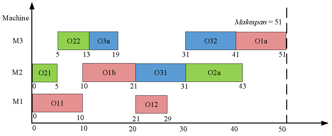
Figure 1. The scheduling solution for the illustrative example.
Symmetry 17 01614 g001
Figure 2. The DT-SLEA framework. (a) The DT-SLEA framework illustrates the interaction between the physical and virtual shop floors. (b) The flow chart of DT-SLEA.
Symmetry 17 01614 g002aSymmetry 17 01614 g002b
Figure 3. An example of encoding scheme.
Symmetry 17 01614 g003
Figure 4. Example of OBX.
Symmetry 17 01614 g004
Figure 5. Example of HMM.
Symmetry 17 01614 g005
Figure 6. Main effects plot of DT-SLEA.
Symmetry 17 01614 g006
Figure 7. Interval plot for EA, DT-EA, SLEA, ε-greedy EA and DT-SLEA.
Symmetry 17 01614 g007
Figure 8. Interval plot for SMA, CC-GP-HH, KLCACO, DRL-Wang, DRL-Zhang and DT-SLEA.
Symmetry 17 01614 g008
Figure 9. Interval plot for DT-SLEA, conventional scheduling strategies and state-of-the-art algorithms.
Symmetry 17 01614 g009
Table 1. Definition of parameters and decision variables of MILP model.
ParameterDefinition
n Job number
m Total number of machines
i   , i Job indices
j , j Operation indices
k , k Machine indices
I Job set, I = 1 , 2 , , n
n i Number of operations for job i  
n i S C O Number of SCOs for job i  
J i Operation set for job i   , J i = 1 , 2 , , n i
J i S C O SCOs set for job i   , J i S C O = 1 , 2 , , n i S C O
O i , j The j th operation of job i  
K i , j The set of eligible machines for operation O i , j . Its size is 1.
p t i , j , k The time required for process O i , j on machine k.
M A large positive number
Decision variables
A i , j , i , j 0–1 decision variable, if O i , j is processed before operation O i , j , A i , j , i , j = 1 ; otherwise, A i , j , i , j = 0 .
B i , j , j 0–1 decision variable, if operation O i , j is processed before operation O i , j , B i , j , j = 1 ; otherwise, B i , j , j = 0 .
C i , j Continuous decision variable, it denotes the starting time of the operation O i , j .
C max Continuous decision variables, it denotes the makespan.
Table 2. Experimental results of the MILP model.
InstancesMILP Model
CmaxTime
JSPDS017395.07
JSPDS028272.78
JSPDS037443.10
JSPDS0485611.91
JSPDS0572118.56
JSPDS0680420.21
JSPDS0730453600
JSPDS0847873600
JSPDS0945763600
JSPDS1043313600
JSPDS1147813600
JSPDS1251943600
JSPDS1348043600
JSPDS1451473600
JSPDS1545453600
JSPDS1668833600
JSPDS1773143600
JSPDS1887483600
JSPDS1992293600
JSPDS2081473600
Table 3. Comparison results of EA, DT-EA, SLEA, ε-greedy EA and DT-SLEA.
InstanceEADT-EASLEAε-Greedy EADT-SLEA
BestAveBestAveBestAveBestAveBestAve
JSPDS010.000.000.000.000.000.000.000.000.000.00
JSPDS020.000.000.000.000.000.000.000.000.000.00
JSPDS030.000.000.000.000.000.000.000.000.000.00
JSPDS040.000.000.000.000.000.000.000.000.000.00
JSPDS050.000.000.000.000.000.000.000.000.000.00
JSPDS060.000.000.000.000.000.000.000.000.000.00
JSPDS071.982.010.560.630.580.640.931.730.000.00
JSPDS081.851.900.590.620.570.611.461.490.000.00
JSPDS091.231.960.630.650.500.660.881.350.000.00
JSPDS101.241.930.600.610.590.841.531.620.000.00
JSPDS111.941.230.550.670.920.661.221.700.000.00
JSPDS121.571.200.640.970.630.520.761.360.000.00
JSPDS131.972.200.580.590.620.631.422.740.000.00
JSPDS141.721.480.590.620.750.661.101.520.000.00
JSPDS151.952.020.610.640.590.651.481.930.000.00
JSPDS161.431.290.820.580.570.520.861.150.000.00
JSPDS171.301.420.600.750.870.610.901.090.000.00
JSPDS181.832.580.580.610.620.640.831.290.000.00
JSPDS191.341.470.560.600.600.630.741.120.000.00
JSPDS201.871.230.620.970.580.651.471.310.000.00
Mean1.161.200.430.480.450.450.781.070.000.00
Table 4. Wilcoxon test for DT-SLEA and other variant algorithms.
DT-SLEA
VS
R+/R−p-ValueRemark
EA105/00.0001<0.05
DT-EA105/00.0001<0.05
SLEA105/00.0001<0.05
ε-greedy EA105/00.0001<0.05
Table 5. Comparison results of SMA, CC-GP-HH, KLCACO, DRL-Wang, DRL-Zhang and DT-SLEA.
InstanceSMACC-GP-HHKLCACODRL-WangDRL-ZhangDT-SLEA
BestAveBestAveBestAveBestAveBestAveBestAve
JSPDS010.000.000.000.000.000.000.000.000.000.000.000.00
JSPDS020.000.000.000.000.000.000.000.000.000.000.000.00
JSPDS030.000.000.000.000.000.000.000.000.000.000.000.00
JSPDS040.000.000.000.000.000.000.000.000.000.000.000.00
JSPDS050.000.000.000.000.000.000.000.000.000.000.000.00
JSPDS060.000.000.000.000.000.000.000.000.000.000.000.00
JSPDS071.791.961.621.971.921.474.367.344.146.640.000.00
JSPDS081.211.341.531.951.891.944.116.323.425.760.000.00
JSPDS091.351.481.931.961.741.972.293.313.585.940.000.00
JSPDS101.231.921.251.411.241.361.822.303.605.000.000.00
JSPDS111.371.281.421.241.782.264.025.963.884.240.000.00
JSPDS121.261.901.451.921.201.402.114.603.636.020.000.00
JSPDS131.781.341.641.971.421.981.564.593.015.400.000.00
JSPDS141.211.931.291.401.891.943.313.393.693.960.000.00
JSPDS151.451.941.361.821.741.971.822.314.135.170.000.00
JSPDS161.671.471.231.241.471.232.085.443.716.440.000.00
JSPDS171.981.231.461.471.911.974.296.592.314.980.000.00
JSPDS181.331.021.391.341.871.912.675.133.405.830.000.00
JSPDS191.921.721.471.271.742.002.923.462.172.510.000.00
JSPDS201.831.921.351.961.921.934.085.302.342.770.000.00
Mean1.07 1.121.021.151.191.272.073.302.353.530.000.00
Table 6. Wilcoxon test for DT-SLEA and other state-of-the-art algorithms.
DT-SLEA
VS
R+/R−p-ValueRemark
SMA105/00.0001<0.05
CC-GP-HH105/00.0001<0.05
KLCACO105/00.0001<0.05
DRL-Wang105/00.0001<0.05
DRL-Zhang105/00.0001<0.05
Table 7. Comparison results of FIFO, LWKR, MWKR, SMA, CC-GP-HH, KLCACO, DRL-Wang, DRL-Zhang and DT-SLEA in the four real-world production cases.
AlgorithmCase1Case2Case3Case4
BestAveBestAveBestAveBestAve
FIFO7.899.1011.9113.3212.5315.0613.4414.85
LWKR12.3718.4214.3418.8512.8813.4411.2712.13
MWKR10.2316.8212.5918.8011.2613.0810.6312.74
SMA0.000.006.788.487.059.287.4212.16
CC-GP-HH0.000.006.918.027.689.867.9010.78
KLCACO0.000.005.027.076.178.397.159.28
DRL-Wang0.000.009.4012.169.8612.898.0713.08
DRL-Zhang0.000.008.0712.017.0511.797.1312.59
DT-SLEA0.000.000.000.000.000.000.000.00
Disclaimer/Publisher’s Note: The statements, opinions and data contained in all publications are solely those of the individual author(s) and contributor(s) and not of MDPI and/or the editor(s). MDPI and/or the editor(s) disclaim responsibility for any injury to people or property resulting from any ideas, methods, instructions or products referred to in the content.