Abstract
Many parametric models can be enriched by introducing additional parameters through transmutation, mixing, or compounding techniques. In this paper, we develop the framework of doubly generalized transmutation models (DGTMs), obtained by the repeated application of rank transmutation maps and their generalizations. We show that several flexible families already available in the literature can be reinterpreted as instances of double or multiple transmutation, thus unifying apparently disparate constructions under a common perspective. A key feature of DGTMs is their ability to flexibly control symmetry through parameterization, enabling more accurate modeling of asymmetric or heavy-tailed phenomena. We also discuss the potential extension of these models to the bivariate case. In addition, we introduce the gentransmuted R package, Version 1.0, which provides routines for data generation, parameter estimation, and model comparison for generalized transmutation models. Two real data applications illustrate the practical advantages of this approach, highlighting improved model fit relative to classical alternatives. Our results underscore the value of transmutation-based methods as a systematic tool for generating flexible probability distributions and advancing their computational implementation.
1. Introduction
The concept of rank transmutation maps (RTMs) was first introduced by Shaw and Buckley [1,2], who proposed quadratic rank transmutation map (QRTM) as a mechanism to generate new distributions from a baseline model. Specifically, they considered cumulative distribution functions (cdfs) of the form
where denotes the baseline cdf to be extended. This can be rewritten as , where , , is itself a cdf indexed by . Subsequent generalizations have considered replacing G with a broader class of parametric distribution functions supported on , leading to what we call general transmutation models, and which was duly documented, for example, by Alzaatreh et al. [3].
Based on this, a doubly generalized transmutation model (DGT) is defined as
where is the baseline family, and , are parametric families of distribution functions supported on . Extensions to triply or multiply generalized transmutation models naturally follow from further compositions. While these constructions can alternatively be viewed simply as compositions of distributions, the terminology of “transmutation” emphasizes their connection with the seminal work of Shaw and Buckley. Note that the cdf in Equation (1) should be extended to the case where and have support different from , considering a new cdf as
where and are ad hoc functions defined from to the corresponding support of and , respectively, which would be a generalization of the idea used to extend distributions used in [3]. However, we will consider the specific case described through Equation (1).
As noted by Tahir and Cordeiro [4], related modeling strategies include scale-mixture constructions, compounding schemes based on probability generating functions, and several models that can be interpreted as special cases of doubly generalized transmutation models. Indeed, most of the flexible families cataloged in their survey can be reinterpreted as instances of double or multiple transmutation.
Recent contributions have reinforced the practical value of QRTM-based approaches. For example, Yedlapalli et al. [5] applied QRTM to the semicircular exponential stereographic distribution, introducing the transmuted semicircular distribution and demonstrating its superior adaptability for modeling geological data. Likewise, Shala and Merovci [6] proposed a three-parameter inverse Rayleigh distribution within the generalized transmuted family, establishing its robustness through extensive theoretical results and empirical applications. These works, together with the foundational studies of [1,2], underscore the ongoing importance of transmutation methods as powerful tools for extending classical probability distributions and improving their empirical performance. Other contributions include the transmuted odd Fréchet-G distribution proposed by Badr et al. [7] and the record-based transmuted Rayleigh distribution of order 3, as presented by Merovci [8]. Together, these works highlight the growing importance of transmutation methods as powerful tools for extending classical probability models and enhancing their practical performance. The primary objective of this paper is to demonstrate that certain generalizations already existing in the literature can be viewed as part of this double transmutation, while also providing a computational alternative associated with these models. The possible generalization of double transmutation to the bivariate case will also be addressed tangentially.
The paper proceeds as follows. In Section 2, we demonstrate the doubly generalized transmutation model with some examples and a selection of examples that can be considered as multiple generalized transmuted distributions. In Section 3, we present multiple transmutations and discuss bivariate transmuting models. In Section 4, we present some computational aspects of the gentransmuted package [9], along with a simulation study. In Section 5, we show two applications to real data. Finally, in Section 6, we will highlight how many of the models listed can be recognized as examples of multiply generalized transmuted models.
2. DGT Distributions
Definition 1 (Doubly Generalized Transmuted Distribution).
Let denote a baseline family of univariate distributions that we aim to make more flexible. Consider two parametric families of univariate distributions supported on , denoted by and .
The resulting family of doubly generalized transmuted distributions, which will be denoted as model, is defined as
For this extended family to include as a special case, it is necessary that both and include the standard uniform distribution as a member. As mentioned in the introduction, such models could alternatively be referred to as multiply compounded models, omitting any explicit reference to transmutation.
Remark 1.
Several well-known distribution families arise as particular cases of Definition 1 when specific choices of and are made. For example, setting , defined below, and leads to the classical transmuted distributions of Shaw and Buckley [1]. Likewise, choosing or produces exponentiated-type distributions [10]. In addition, using Marshall–Olkin-type functions, i.e., mappings of the form
as originally introduced by Marshall and Olkin [11], generates Marshall–Olkin extended families. These models are widely used because they allow for tractable survival functions and hazard rate modifications. Finally, notice that if both and are chosen as the identity function, then the construction trivially reduces to the baseline distribution . Thus, the proposed framework provides a unifying structure that encompasses transmuted, exponentiated, and Marshall–Olkin families, along with many other extensions frequently encountered in the literature.
Definition 2 (Transmuting functions).
A transmuting function is a distribution function supported on , depending on a parameter (or vector of parameters) , such that the standard uniform distribution is included as a special case.
Five popular choices for the transmuting functions and are:
- 1.
- The original transmuting function [1]:Note that if , this reduces to the distribution.
- 2.
- The exponentiating (EXP) function:If , this is the distribution; if , it corresponds to the distribution of the maximum of n i.i.d. variables.
- 2A.
- The exponentiating function of the second kind (EXP2):For , this yields the distribution; for , it is the distribution of the minimum of n i.i.d. variables.
- 3.
- The Marshall-Olkin function [11]:When , this simplifies to the distribution.
- 3A.
- The second kind Marshall-Olkin (MO2) function:Again, yields the distribution.
Remark 2.
The MO and MO2 functions, if , can be interpreted as arising from the maximum and minimum, respectively, of a sample of geometrically distributed size of variables. If the sample size instead follows a zero-truncated Poisson distribution, we obtain two new transmuting functions:
Similarly, using logarithmic sample sizes leads to:
- 4.
- The Kumaraswamy function [12]:If , this corresponds to .It can also be expressed as a composition of two exponentiating functions:By reversing the order of composition, we define a second-kind Kumaraswamy function:
- 5.
- Mixtures. Granzotto and Louzada [13] observed that the SB transmutation function can be expressed as a convex combination of the maximum and minimum of a size-two sample from :where .They also explored convex combinations of multiple order statistics. More recently, Balakrishnan and He [14] proposed convex combinations of record value distributions (both lower and upper records). In general, convex combinations of any set of transmuting functions can be considered to generate more flexible transformation families.
Figure 1 presents the PDF for the exponential (exp) distribution and some extensions from these models based on the EXP and SB models. Note that the PDF of the exponential model is monotone, whereas the extensions provide non-monotonic PDFs in all the cases.
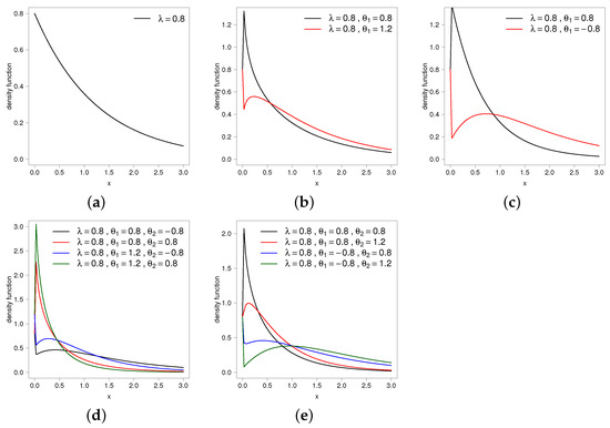
Figure 1.
Plot of PDFs for different extensions of the exponential distribution: (a) exp; (b) EXP-exp; (c) SB-exp; (d) EXP-SB-exp and (e) SB-EXP-exp.
It is often convenient to restrict attention to transmuting functions with simple closed-form expressions for both the function and its first derivative. This is particularly helpful for inference. For this reason, the Kumaraswamy function may be preferred over the Beta distribution, which lacks a simple closed-form for its CDF.
For simulation purposes, it is especially useful if both the transmuting functions and the baseline distribution have analytical inverse functions.
Note that the MO function with is the probability generating function (PGF) of a geometric random variable with parameter (taking values in ).
Similarly, the PGF of any positive integer-valued distribution may be used as a transmuting function. However, acceptable transmuting functions are not limited to PGFs with non-negative power series coefficients.
Another useful class of PGFs arises from the negative binomial distribution:
where and . This function is a composition of the EXP and MO functions. Hence, the parameter p can be extended to .
Examples of Multiple Generalized Transmuted Distributions
The generalized transmutation approach, in which a family of generalized transmutation functions is applied to a parametric baseline family of distributions, yields an enriched extended family. Provided that the transmutation family includes the uniform distribution, this guarantees that the extended family will fit the data at least as well as the baseline, i.e., a non-worse maximized likelihood on the same data, but not necessarily a better predictive performance. However, the question of whether the improvement in fit is statistically significant must be carefully assessed.
Repeated applications of transmutation functions can produce increasingly flexible models, consistently enhancing the fit to the data. Naturally, this process should not be carried to excess. Nevertheless, rather complex models constructed from multiple transmutation functions have already been proposed in the literature. We cite below a selection from the extensive list compiled by Tahir and Cordeiro [4]:
- Transmuted Complementary Exponentiated Weibull-Geometric (TCEWG) model
- Transmuted Complementary Weibull-Geometric (TCWG) model
- Exponentiated Transmuted Weibull-Geometric (ETWG) model
- Exponentiated Geometric G-Poisson (EGGP) model
- Complementary Extended Weibull Power Series (CEWPS) models
- Complementary Exponentiated Weibull-Logarithmic (CEWLn) model
- Complementary Exponentiated Power Lindley-Poisson (CEPLP) model
- Poisson Generalized Linear Failure Rate (PGLFR) model
3. Multiple Transmutation
Several transmutation operations can be applied to a given baseline family of distributions to obtain ever more flexible models with more and more parameters. Alternatively, one can observe that compositions of two or more transmutation functions are again (albeit more complicated) transmutation functions. For example, we might consider the composition.
The three transmutation functions used here can be composed in different orders, leading to six distinct models. Moreover, the composition of more than three transmutation functions could be considered. Clear guidelines on how to select from the myriad of available models are lacking at this time.
Transmuting Bivariate Models
Given the success in generating flexible univariate models documented above, it is natural to consider the possibility of using the transmuting strategy to generate flexible bivariate (and perhaps multivariate) models.
To this end, consider a baseline family of bivariate distributions that we wish to make more flexible. Let be a parametric family of univariate distributions with support , i.e., a family of transmutation functions.
In one dimension, it is evident that compounding a transmutation function with any distribution function leads to a valid distribution function. Can the same thing be said in higher dimensions? Leaving aside parameters for the moment, we ask whether, when is a valid bivariate distribution function and if is a transmutation function, it is necessarily true that is a valid bivariate distribution function? Or must some conditions be satisfied for this to happen?
Since F is a valid bivariate distribution function, we know that for any four real numbers satisfying and , we have
Is it then true that for such we also have
A little investigation will confirm that this will not always be true. For example, suppose that our joint distribution F is such that, for four numbers satisfying and we have
so that
Now consider the particular transmutation function . In this case, we will have
So, in this case, is not a valid joint distribution function.
A positive result is obtainable if we assume that F is absolutely continuous and that the transmuting function G is a convex distribution function as noted in the following theorem.
Theorem 1.
If the joint distribution function is absolutely continuous and if the transmuting function G is a convex distribution function with support (0, 1), then is a well-defined bivariate distribution function.
Proof.
Since we assume absolute continuity of its density, denoted by , can be obtained as
The density of the putative transmuted distribution denoted by will be of the form
It is this expression which must be shown to be non-negative. However, we know that is non-negative, as are and , so that in addition to requiring that be non-negative (which we know is true), we must also require that be non-negative, i.e., that G is convex, which was assumed in the hypothesis of the theorem. Using the fact that G is a valid distribution function with support , we can conclude that has a non-negative density and has total variation equal to 1, i.e., that it is a valid bivariate distribution function. □
So the conclusion is that there will be no problem as long as is convex. We note that our earlier example, in which a problem was encountered, dealt with a choice for G of the form which was concave rather than convex.
Note that if is the probability generating function of a non-negative integer-valued random variable, then it will be convex. Thus, for example, MO functions can be used in the bivariate case provided we restrict the parameter to the interval .
Indeed, there will be no problems in higher dimensions, provided that G is a generating function. This is because we may think of a sequence of independent identically distributed k-dimensional random variables with common distribution function and an independent integer-valued random variable N with generating function G. Suppose we define , then it can be readily verified that the distribution function of is given by which is then necessarily a valid k-dimensional distribution function. The required conditions when G is not assumed to be a generating function are more complex.
In general, we can consider parametric families of multivariate distributions that are subjected to parametric families of double transmutations, and these will be guaranteed to be valid models provided that all the transmutation functions involved are generating functions of non-negative integer-valued random variables. Such models will be of the form.
where and are parametric families of generating functions, and F is a parametric family of k-dimensional distributions.
Although it is conceptually possible to consider triple transmutation (or indeed, k-fold transmutation) applied to multivariate distributions, it is not envisioned that such models would be much used in practice.
4. Computational Implementation and Simulation Study
In this section, we present the computational implementation of the models, as well as a brief simulation study to assess the performance of the maximum likelihood (ML) estimators in finite samples.
4.1. Computational Aspects
The gentransmuted package [9] of R [15] includes the computational implementation for the GDT class of models. To fit a given model in this class using the gentransmuted package, the following commands can be executed
- 1.
- Install and load the necessary packages:

- 2.
- Load your data into R (say y).
- 3.
- To estimate a specific combination of distribution (dist) and and (comp1 and comp2, respectively), which are optional. For example, for the exponential model as baseline distribution with the and equal to EXP and MO models, we use the following sentence

The package also includes the choose.compound function, which performs all the combinations among dist, comp1, and comp2 and presents the results in a descendant order based on the Akaike Information Criterion (AIC, [16]) or the Bayesian Information Criterion (BIC, [17]). Depending on the nature of the data, the following options are available.
- Positive data: exponential, gamma, log-normal, BS, and Pareto II.
- Unit data: beta and Kumaraswamy.
- Real data: normal, Cauchy, logistic and Gumbel.
For comp1 and comp2, all the combinations among the EXP, EXP2, MO, MO2, and SB models are considered, in addition to the case where they are specified as NULL. For instance, if the data are positive and the AIC is used as a selection criterion, the function is used as follows

In addition, functions to compute the PDF, CDF, quantile function, and drawn values are available as dcompound, pcompound, qcompound, and rcompound, respectively, specifying the arguments dist, comp1, comp2, and the corresponding parameters.
4.2. Simulation Study
In this subsection, we present a brief simulation study to assess the performance of the maximum likelihood (ML) estimators obtained with the gentransmuted package. We consider two baseline distributions f: the exponential distribution with parameter 1.5 and the Lomax distribution with parameters 1.5 and 2; two models for (EXP and MO); two values for the parameter (0.75 and 1.2); and sample sizes .
For each combination of f, , , and sample size, we generate 1000 replicates using the rcompound function and estimate parameters with the estimate.compound function. Table 1 summarizes the results based on these replicates: the mean bias (Bias), the mean of the standard errors (SE), the root of the mean squared error (RMSE), and the 95% coverage probability (CP) based on the asymptotic distribution of the ML estimators.

Table 1.
Estimated bias, mean standard error (SE), root mean squared error (RMSE), and 95% coverage probability (CP) for different combinations of baseline distribution f (exponential and Lomax), transmutation function G (EXP and MO), parameter (0.75 and 1.2), and sample sizes ().
The results suggest that the bias of the estimators is acceptable in most cases considered and decreases as the sample size increases. Additionally, the SE and RMSE values are close, indicating that the variance of the estimators is well estimated. Coverage probabilities are close to nominal levels, especially for . The exception is for the combination of Lomax and MO for f and , where the estimators need a larger sample size to obtain desirable properties. This is probably because the Lomax distribution is a heavy-tailed distribution, which is inherited by the respective composite model.
5. Applications of a Multiple Transmutation with Real Data
Let X be a continuous random variable with pdf and cdf . The objective is to extend the pdf using multiple transmutation, as follows.
5.1. First Transmutation
The corresponding PDFs of the singly and doubly transmuted distributions are:
where and are shape parameters.
Log-Likelihood Function
Given a random sample from , the log-likelihood function is:
and can be maximized using the gentransmuted package [9].
5.2. Second Transmutation
The corresponding PDFs are:
with and .
Log-Likelihood Function
For a sample from , the log-likelihood is:
5.3. Data I
For this analysis, we use the fatigue life dataset of Kevlar 373/epoxy specimens subjected to 90% of the ultimate stress until failure. The data, originally reported by Andrews et al. [18] and Barlow et al. [19], contain exact failure times: 0.0251, 0.0886, 0.0891, 0.2501, 0.3113, 0.3451, 0.4763, 0.5650, 0.5671, 0.6566, 0.6748, 0.6751, 0.6753, 0.7696, 0.8375, 0.8391, 0.8425, 0.8645, 0.8851, 0.9113, 0.9120, 0.9836, 1.0483, 1.0596, 1.0773, 1.1733, 1.2570, 1.2766, 1.2985, 1.3211, 1.3503, 1.3551, 1.4595, 1.4880, 1.5728, 1.5733, 1.7083, 1.7263, 1.7460, 1.7630, 1.7746, 1.8275, 1.8375, 1.8503, 1.8808, 1.8878, 1.8881, 1.9316, 1.9558, 2.0048, 2.0408, 2.0903, 2.1093, 2.1330, 2.2100, 2.2460, 2.2878, 2.3203, 2.3470, 2.3513, 2.4951, 2.5260, 2.9911, 3.0256, 3.2678, 3.4045, 3.4846, 3.7433, 3.7455, 3.9143, 4.8073, 5.4005, 5.4435, 5.5295, 6.5541, 9.0960.
Table 2 presents descriptive statistics of the dataset, including the sample coefficient of skewness (CS) and coefficient of kurtosis (CK). The choose.compound function is used to select an appropriate combination of distribution, , and for modeling these data.
Table 2.
Descriptive statistics for fatigue life data.
Estimation and Model Selection
We illustrate the use of multiple transmutations with a real data set. We use the choose.compound function, as explained in the previous section, to choose a model for positive data. The output for the first six models is as follows:

Table 3 presents the results for the selected model. Figure 2 displays the Q-Q plots for the selected model. From them, we calculated the quantile residuals (QRs), which—if the model is appropriate for the data—should behave like a sample from the standard normal distribution (see [20]). This can be validated using traditional tests for normality such as the Anderson–Darling (AD), Cramér–von Mises (CVM), and Shapiro–Wilk (SW) tests.
Table 3.
Parameter estimates and standard errors (SE), AIC and BIC values for the exponential-MO-SB model.
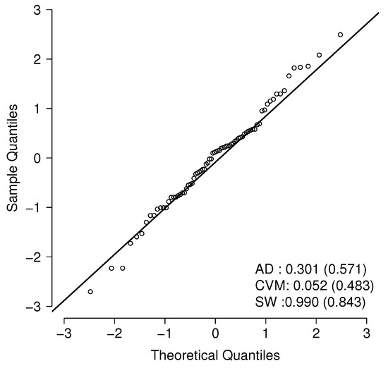
Figure 2.
Q-Q plot for the exponential-MO model.
In Figure 2, the p-values for the normality tests (AD, CVM, and SW) of the QRs for the two best models are shown below the corresponding Q-Q plots. In the and models, the QRs appear to behave like standard normal variates. This supports the earlier claim that model provides the best fit to the data.
5.4. Data II
In this subsection, we illustrate the use of multiple transmutations with another real data set. For this application, we use the Pareto II distribution as the baseline distribution (see Arnold, [21]). A random variable X has a Pareto II distribution if its cumulative distribution function (CDF) is given by
and its corresponding probability density function (PDF) is
where , is a scale parameter, and is a shape (or inequality) parameter. We denote this as .
This dataset originates from the Survey of Consumer Finances (SCF), a nationally representative sample that provides extensive information on the assets, liabilities, income, and demographic characteristics of U.S. households. It includes a random sample of 500 households with positive incomes interviewed in the 2004 survey. The variable of interest is the annual family income (in thousands of U.S. dollars), divided by the number of household members. The data can be accessed from the Federal Reserve’s webpage: https://www.federalreserve.gov/econres/scfindex.htm (accessed on 31 August 2025).
The descriptive statistics corresponding to this dataset are shown in Table 4. The very high kurtosis coefficient indicates that the dataset has a heavy right tail, motivating the use of the Pareto II distribution as the baseline model.
Table 4.
Descriptive statistics for income data.
Estimation and Model Selection
Codes to replicate this example using the gentransmuted package are provided in the Appendix A. In Table 5, the maximum likelihood estimates of the parameters of the five competing models are displayed. To compare the models—Pareto II, , , , and —we use the Akaike Information Criterion (AIC) and the Bayesian Information Criterion (BIC). Table 5 also includes the AIC and BIC values for each model.
Table 5.
Parameter estimates, AIC, and BIC values for the models.
In particular, the probability density function (pdf) of is
the pdf of is
the pdf of is
and the pdf of is
where is a scale parameter, and , , and are shape parameters.
We observe from the AIC and BIC values in Table 5 that each application of generalized transmutation yields an improvement in model fit. Model demonstrates the best performance among the five models. Finally, Figure 3 presents the Q–Q plot for the QRs, suggesting that the and models are appropriated for this data set.

Figure 3.
Q–Q plots for models (left panel) and (right panel). p-values of normality tests (AD, CVM, WS) for the QRs are indicated below each plot.
6. Final Remark
The results presented in this work highlight the advantages of using generalized transmutation techniques to construct flexible distribution families. As demonstrated in Section 5, each level of transmutation—whether through exponentiation, convex combinations, or the incorporation of generator functions—tends to enhance the goodness-of-fit to real data. This is evidenced by model outperforming the others according to AIC, BIC, and residual analysis.
Future work should focus on a more detailed study of specific members within the proposed family that may possess closed-form expressions for key distributional characteristics such as the mean, quantiles, or mode. Additionally, it would be valuable to extend the regression framework to cover these special cases, enabling their application in modeling conditional relationships in practical contexts.
Author Contributions
Conceptualization, B.C.A. and H.W.G.; methodology, B.C.A. and H.W.G.; software, Y.M.G. and D.I.G.; validation, Y.M.G. and D.I.G.; formal analysis, Y.M.G. and H.W.G.; investigation, B.C.A. and D.I.G.; data curation, Y.M.G. and D.I.G.; writing—original draft preparation, B.C.A.; writing—review and editing, Y.M.G., D.I.G. and H.W.G.; visualization, D.I.G. and H.W.G.; supervision, B.C.A. and H.W.G. All authors have read and agreed to the published version of the manuscript.
Funding
This research received no external funding.
Data Availability Statement
The original contributions presented in the study are included in the article, further inquiries can be directed to the corresponding author.
Conflicts of Interest
The authors declare no conflicts of interest.
Appendix A
In this section, we include the codes in R related to the simulation study and the second application.
Appendix A.1. Codes for the Simulation Study
install.packages(‘‘gentransmuted’’)
library(gentransmuted)
set.seed(2100); dist=‘‘exp’’; comp=‘‘EXP’’; n=100; para=1.5; theta1=0.75; replicas=1000
m=1;resultados=c(); real=c(para,theta1)
while(m<=replicas){
y=rcompound(n, dist=dist, comp1=comp1, comp2=comp2, gamma=para[1], theta1=theta1)
aux=estimate.compound(y, dist=dist, comp1=comp1, comp2=comp2,est.var=TRUE)
resultados=rbind(resultados, c(aux$coefficients[,1],aux$coefficients[,2])); m=m+1}
bias.aux=resultados[,1:2]-matrix(real, ncol=length(real), nrow=replicas, byrow=T)
bias=apply(bias.aux, 2, mean); SE=apply(base[,1:2+length(real)],2,mean)
RMSE=sqrt(apply(bias.aux^2,2,mean))
CP.aux=ifelse(bias.aux-1.96*resultados[,sele+length(real)]<0&bias.aux+
1.96*resultados[,sele+length(real)]>0,1,0)
CP=apply(CP.aux,2,mean); c(bias, SE, RMSE, CP)
Appendix A.2. Codes for the First Application
y<-c(0.0251, 0.0886, 0.0891, 0.2501, 0.3113, 0.3451, 0.4763, 0.5650, 0.5671, 0.6566, 0.6748,
0.6751, 0.6753, 0.7696, 0.8375, 0.8391, 0.8425, 0.8645, 0.8851, 0.9113, 0.9120, 0.9836,
1.0483, 1.0596, 1.0773, 1.1733, 1.2570, 1.2766, 1.2985, 1.3211, 1.3503, 1.3551, 1.4595,
1.4880, 1.5728, 1.5733, 1.7083, 1.7263, 1.7460, 1.7630, 1.7746, 1.8275, 1.8375, 1.8503,
1.8808, 1.8878, 1.8881, 1.9316, 1.9558, 2.0048, 2.0408, 2.0903, 2.1093, 2.1330, 2.2100,
2.2460, 2.2878, 2.3203, 2.3470, 2.3513, 2.4951, 2.5260, 2.9911, 3.0256, 3.2678, 3.4045,
3.4846, 3.7433, 3.7455, 3.9143, 4.8073, 5.4005, 5.4435, 5.5295, 6.5541, 9.0960)
choose.compound(y)
Appendix A.3. Codes for the Second Application
y=as.vector(read.table(‘‘Datos2.txt’’,h=F)$V1)
aux1=estimate.compound(y, dist=‘‘paretoII’’)
aux2=estimate.compound(y, dist=‘‘paretoII’’, comp1=‘‘EXP’’)
aux3=estimate.compound(y, dist=‘‘paretoII’’, comp1=‘‘EXP’’, comp2=‘‘SB’’)
aux4=estimate.compound(y, dist=‘‘paretoII’’, comp1=‘‘SB’’)
aux5=estimate.compound(y, dist=‘‘paretoII’’, comp1=‘‘SB’’, comp2=‘‘EXP’’)
aux1;aux2;aux3;aux4;aux5
c(aux1$AIC, aux2$AIC, aux3$AIC, aux4$AIC, aux5$AIC)
c(aux1$BIC, aux2$BIC, aux3$BIC, aux4$BIC, aux5$BIC)
References
- Shaw, W.T.; Buckley, I.R.C. The Alchemy of Probability Distributions: Beyond Gram-Charlier & Cornish-Fisher Expansions, and Skew-Normal or Kurtotic-Normal Distributions; Research Report; Wolfgram Memorial Library: Chester, PA, USA, 2007. [Google Scholar]
- Shaw, W.T.; Buckley, I.R.C. The alchemy of probability distributions: Beyond Gram-Charlier expansions, and a skew-kurtotic-normal distribution from a rank transmutation map. arXiv 2009, arXiv:0901.0434. [Google Scholar]
- Alzaatreh, A.; Lee, C.; Famoye, F. A new method for generating families of continuous distributions. Metron 2003, 71, 63–79. [Google Scholar] [CrossRef]
- Tahir, M.H.; Cordeiro, G.M. Compounding of distributions: A survey and new generalized classes. J. Stat. Distrib. Appl. 2016, 3, 13. [Google Scholar] [CrossRef]
- Yedlapalli, P.; Kishore, G.N.V.; Boulila, W.; Koubaa, A.; Mlaiki, N. Toward enhanced geological analysis: A novel approach based on transmuted semicircular distribution. Symmetry 2023, 15, 2030. [Google Scholar] [CrossRef]
- Shala, M.; Merovci, F. A New Three-Parameter Inverse Rayleigh Distribution: Simulation and Application to Real Data. Symmetry 2024, 16, 634. [Google Scholar] [CrossRef]
- El-Morshedy, M.; Alshammari, F.S.; Tyagi, A.; Elbatal, I.; Hamed, Y.S.; Eliwa, M.S. Bayesian and Frequentist Inferences on a Type I Half-Logistic Odd Fréchet Class of Distributions. Entropy 2020, 23, 446. [Google Scholar] [CrossRef]
- Merovci, F. A Three-Parameter Record-Based Transmuted Rayleigh Distribution (Order 3): Theory and Real-Data Applications. Symmetry 2025, 17, 1034. [Google Scholar] [CrossRef]
- Gómez, Y.M.; Gómez, H.W.; Arnold, B.C.; Gallardo, D.I. Gentransmuted: Estimation and Other Tools for Generalized Transmuted Models. R Package Version 1.0. 2025. Available online: https://CRAN.R-project.org/package=gentransmuted (accessed on 31 August 2025).
- Gupta, R.C.; Nadarajah, S. Handbook of Exponential and Related Distributions for Engineers and Scientists; Chapman and Hall: Boca Raton, FL, USA; CRC: Boca Raton, FL, USA, 2004. [Google Scholar]
- Marshall, A.W.; Olkin, I. A new method for adding a parameter to a family of distributions with application to the exponential and Weibull families. Biometrika 1997, 84, 641–652. [Google Scholar] [CrossRef]
- Kumaraswamy, P. Generalized probability density function for double-bounded random processes. J. Hydrol. 1980, 462, 79–88. [Google Scholar] [CrossRef]
- Granzotto, D.C.T.; Louzada, F. The transmuted log-logistic distribution: Modeling, inference, and an application to a polled Tabapua race time up to first calving data. Comm. Statist. Theory Methods 2015, 44, 3387–3402. [Google Scholar] [CrossRef]
- Balakrishnan, N.; He, M. A record-based transmuted family of distributions. In Advances in Statistics—Theory and Applications; Emerging Topics in Statistics and Biostatistics; Springer: Cham, Switzerland, 2021; pp. 3–24. [Google Scholar]
- R Core Team. R: A Language and Environment for Statistical Computing; R Foundation for Statistical Computing: Vienna, Austria, 2025; Available online: https://www.R-project.org/ (accessed on 31 August 2025).
- Akaike, H. A new look at the statistical model identification. IEEE Trans. Autom. Control 1974, 19, 716–723. [Google Scholar] [CrossRef]
- Schwarz, G. Estimating the dimension of a model. Ann. Statist. 1978, 6, 461–464. [Google Scholar] [CrossRef]
- Andrews, D.F.; Herzberg, A.M. Data: A Collection of Problems from Many Fields for the Student and Research Worker; Springer Series in Statistics; Springer: New York, NY, USA, 1985. [Google Scholar]
- Barlow, R.E.; Tol, R.H.; Freeman, T. A Bayesian Analysis of Stress-Rupture Life of Kevlar 49/Epoxy Spherical Pressure Vessels; Marcel Dekker: New York, NY, USA, 1984. [Google Scholar]
- Dunn, P.K.; Smyth, G.K. Randomized Quantile Residuals. J. Comput. Graph. Stat. 1996, 5, 236–244. [Google Scholar] [CrossRef]
- Arnold, B.C. Pareto Distributions, 2nd ed.; Monographs on Statistics & Applied Probability; Chapman and Hall: Boca Raton, FL, USA; CRC: Boca Raton, FL, USA, 2015. [Google Scholar]
Disclaimer/Publisher’s Note: The statements, opinions and data contained in all publications are solely those of the individual author(s) and contributor(s) and not of MDPI and/or the editor(s). MDPI and/or the editor(s) disclaim responsibility for any injury to people or property resulting from any ideas, methods, instructions or products referred to in the content. |
© 2025 by the authors. Licensee MDPI, Basel, Switzerland. This article is an open access article distributed under the terms and conditions of the Creative Commons Attribution (CC BY) license (https://creativecommons.org/licenses/by/4.0/).