A Nonconvex Fractional Regularization Model in Robust Principal Component Analysis via the Symmetric Alternating Direction Method of Multipliers

Abstract

This paper addresses the NP-hard problem of solving the rank of a matrix in Robust Principal Component Analysis (RPCA) by proposing a nonconvex fractional regularization approximation. Compared to existing convex regularization (which often yields suboptimal solutions) and nonconvex regularization (which typically requires parameter selection), the proposed model effectively avoids parameter selection while preserving scale invariance. By introducing an auxiliary variable, we transform the problem into a nonconvex optimization problem with a separable structure. We use a more flexible Symmetric Alternating Direction Method of Multipliers (SADMM) to arrive at a solution and provide a rigorous convergence proof. In numerical experiments involving synthetic data, image recovery, and foreground–background separation for surveillance video, the proposed fractional regularization model demonstrates high computational accuracy, and its performance is comparable to that of many state-of-the-art algorithms.

1. Introduction

Over the past few decades, Robust Principal Component Analysis (RPCA), a crucial analytical tool, has been widely applied in various fields (see references [1,2,3,4,5,6,7]) to reconstruct low-rank matrices X and sparse matrices Y from observed datasets $M\in {\mathbb{R}}^{m\times n}(m\le n)$. In practical applications, M typically represents high-dimensional datasets such as surveillance videos, recognized images, or text documents; X denotes the primary structural components of the data (e.g., static backgrounds in surveillance footage, texture features in images, or common vocabulary across documents); while Y represents anomalous components (such as moving objects in videos, image noise, or keywords distinguishing different documents). Given the low rank and sparse nature of the underlying data, we mathematically formulate RPCA as the following model:

$$\underset{X,Y}{min}rank\left(X\right)+\mu {\parallel Y\parallel }_0,\mathrm{s}.\mathrm{t}.X+Y=M,$$

(1)

where $rank(·)$ (resp., ${\parallel ·\parallel }_0$ ) denotes the rank (resp., is the number of non-zeros) of the matrix, and $\mu >0$ is a trade-off parameter. However, due to the discontinuity of the model, it is NP-hard.

1.1. Related Work

In recent years, theoretical exploration and algorithm design for problem (1) have sparked a significant research boom in academia. Most studies focus on convex and nonconvex relaxation strategies for RPCA. Wright et al. [8] conducted a systematic and comprehensive analysis of the convex relaxation model for problem (1) under relatively mild assumptions. The details of which are as follows:

$$\underset{X,Y}{min}{\parallel X\parallel }_{*}+\mu {\parallel Y\parallel }_1,\mathrm{s}.\mathrm{t}.X+Y=M,$$

(2)

where ${\parallel ·\parallel }_{*}$ represents the nuclear norm (calculated as the sum of all its non-zero singular values of a matrix) to promote the low-rank component of M, and ${\parallel ·\parallel }_1$ denotes the ${\mathsf{\ell }}_1$ norm (calculated as maximum of the absolute sums of all columns of a matrix) to encourage the sparse component of M.

For practical applications, and in view of the incomplete observation characteristics of M, Tao and Yuan [9] further extended model (2), and the specific mathematical form is as follows:

$$\underset{X,Y}{min}{\parallel X\parallel }_{*}+\mu {\parallel Y\parallel }_1,\mathrm{s}.\mathrm{t}.P_{\mathrm{\Omega }}(X+Y)=P_{\mathrm{\Omega }}\left(M\right),$$

(3)

where $\mathrm{\Omega }$ is a subset of the index set $\{1,2,\cdots ,m\}\times \{1,2,\cdots ,n\}$, representing the observable entries, and $P_{\mathrm{\Omega }}:{\mathcal{R}}^{m\times n}\to {\mathcal{R}}^{m\times n}$ is the orthogonal projection onto the span of matrices vanishing outside of $\mathrm{\Omega }$ so that the $ij$-th entry of $P_{\mathrm{\Omega }}\left(X\right)$ is $X_{ij}$ if $(i,j)\in \mathrm{\Omega }$, otherwise it is zero.

Models (2) and (3) have a concise and clear architecture with a convenient solution process [9]. Under the assumption of incoherence, the convex model is able to recover the low-rank and sparse components with very high probability [1]. However, the model suffers from two limitations that restrict its applicability. Firstly, in real-world applications, the underlying matrices may lack the necessary incoherence guarantees [1] and the data may be severely compromised. In this scenario, the global optimal solution of the model may deviate significantly from the true value. Secondly, RPCA performs an equal scaling reduction for all singular values. The nuclear norm is essentially the ${\mathsf{\ell }}_1$ norm of the singular values, and the ${\mathsf{\ell }}_1$ norm has a shrinkage property, which will lead to estimates [10,11] that are biased. This means that the nuclear norm imposes an overpenalty on larger singular values and may end up obtaining only a severely erroneous solution. Based on this, a variety of nonconvex relaxations of rank functions have been proposed. For convenience, we provide the general expression for nonconvex regularization as follows (for specific details, please refer to Table 1):

$$\underset{X,Y}{min}\sum _{i=1}^{m}h\left({\sigma }_i\left(X\right)\right)+\mu {\parallel Y\parallel }_1,\mathrm{s}.\mathrm{t}.P_{\mathrm{\Omega }}(X+Y)=P_{\mathrm{\Omega }}\left(M\right),$$

(4)

where ${\sigma }_i$ denotes the i-th singular value of matrix X.

Table 1. Nonconvex regularized functions.

$h:{\mathbb{R}}_{+}\to \mathbb{R}$ with parameters $\lambda >0$, $\gamma >0$ and $0<p<1$
SCAD [10]	$h\left(t\right)=\left\{\begin{array}{cc}\lambda t,\hfill & \mathrm{if}t\le \lambda \hfill \\ {\displaystyle \frac{-t^2+2\gamma \lambda t-{\lambda }^2}{2(\gamma -1)}},\hfill & \mathrm{if}\lambda <t\le \gamma \lambda \hfill \\ {\displaystyle \frac{{\lambda }^2(\gamma +1)}{2}},\hfill & \mathrm{if}t>\gamma \lambda \hfill \end{array}\right.$
MCP [11]	$h\left(t\right)=\left\{\begin{array}{cc}\lambda t-{\displaystyle \frac{t^2}{2\gamma }},\hfill & \mathrm{if}t<\gamma \lambda \hfill \\ {\displaystyle \frac{\gamma {\lambda }^2}{2}},\hfill & \mathrm{if}t\ge \gamma \lambda \hfill \end{array}\right.$
Clapped ${\mathsf{\ell }}^1$ [12]	$h\left(t\right)=\left\{\begin{array}{cc}\lambda t,\hfill & \mathrm{if}t<\gamma \hfill \\ \lambda \gamma ,\hfill & \mathrm{if}t\ge \gamma \hfill \end{array}\right.$
LSP [13]	$h\left(t\right)=\lambda log(1+{\displaystyle \frac{t}{\gamma }})$
Logarithm [14]	$h\left(t\right)={\displaystyle \frac{\lambda log(\gamma t+1)}{log(\gamma +1)}}$
Sp [15]	$h\left(t\right)=\lambda t^p$
SCp [16]	$h\left(t\right)=\left\{\begin{array}{cc}{\displaystyle \frac{1}{2}}{(t-\delta )}^2+\lambda {\gamma }^p,\hfill & \mathrm{if}t>\gamma \hfill \\ {\displaystyle \frac{1}{2}}{(t-\delta )}^2+\lambda t^p,\hfill & \mathrm{if}t\ge \gamma \hfill \end{array}\right.$
ETP [17]	$h\left(t\right)={\displaystyle \frac{\lambda }{1-exp(-\gamma )}}(1-exp(-\gamma t))$
Geman [18]	$h\left(t\right)={\displaystyle \frac{\lambda t}{t+\gamma }}$
Laplace [19]	$h\left(t\right)=\lambda (1-exp(-{\displaystyle \frac{t}{\gamma }}))$

Numerous experimental results reveal that, with proper parameter settings, model (4) can often achieve superior performance compared to the nuclear norm. However, parameter estimation for nonconvex approximations is too time-consuming in terms of the computational process. Theoretically, a uniform evaluation criterion is lacking for optimal parameter selection. Therefore, the natural question is: is it possible to find a nonconvex model to avoid parameter estimation?

Fortunately, the fractional model (Nuclear/Frobenius, N/F) can effectively fill this research gap. On the one hand, it avoids the time consumption caused by parameter selection during computation. On the other hand, the fractional structure possesses inherent scale invariance, which also distinguishes it from other nonconvex models. Moreover, Gao et al. [20] demonstrated the significant advantage of the fractional model in approximating the rank function through a concrete example. It should be especially emphasized that when the fractional model is applied to the field of vector optimization, it will be reduced to the ${\mathsf{\ell }}_1/{\mathsf{\ell }}_2$ model, and the related applications have been explored in several references [21,22,23,24,25,26,27], which will not be discussed in detail in this paper.

1.2. Problem Description

Inspired by the application of the fractional model to the low-rank matrix recovery problem [20], we constructed the following more general optimization model under the premise of incomplete data observation:

$$\underset{X,Y}{min}{\lambda }_1{\displaystyle \frac{{\parallel X\parallel }_{*}}{{\parallel X\parallel }_F}}+{\lambda }_2{\parallel Y\parallel }_1\mathrm{s}.\mathrm{t}.\mathcal{A}(X+Y)=b,$$

(5)

where ${\parallel ·\parallel }_F$ is the Frobenius norm (calculated as the square root of the sum of the squares of all matrix entries), ${\lambda }_i>0(i=1,2)$ are the balancing parameters of X and Y, $\mathcal{A}\in {\mathbb{R}}^{m\times n}\to {\mathbb{R}}^{m\times n}$ is a linear operator, and $b\in {\mathbb{R}}^{m\times n}$ is an observed vector/matrix. By penalizing the constraint into the objective function, we obtain the following equivalent form of (5):

$$\underset{X,Y}{min}{\lambda }_1{\displaystyle \frac{{\parallel X\parallel }_{*}}{{\parallel X\parallel }_F}}+{\lambda }_2{\parallel Y\parallel }_1+{\displaystyle \frac{1}{2}}{\parallel \mathcal{A}(X+Y)-b\parallel }_F^2.$$

(6)

In comparison to the existing nonconvex models, the proposed model can effectively avoid the suboptimal solution caused by improper parameter selection. In addition, the model is closer to the matrix’s rank and still retains the property of scale invariance.

Through the introduction of a supplementary variable $Z\in {\mathbb{R}}^{m\times n}$, we reconstruct the primitive formulation (6) into the following optimization problem equipped with a separable structure:

$$\begin{array}{cc}\hfill & \underset{X,Y,Z}{min}{\lambda }_1{\displaystyle \frac{{\parallel X\parallel }_{*}}{{\parallel X\parallel }_F}}+{\lambda }_2{\parallel Y\parallel }_1+{\displaystyle \frac{1}{2}}{\parallel \mathcal{A}\left(Z\right)-b\parallel }_F^2\hfill \\ \hfill & \mathrm{s}.\mathrm{t}.\mathrm{X}+\mathrm{Y}=\mathrm{Z}.\hfill \end{array}$$

(7)

Due to the fact that the Alternating Direction Multiplier Method (ADMM) is known to be a very effective algorithmic framework for solving an optimization problem with a separable structure, and inspired by [28], we adopt a more flexible Symmetric ADMM (SADMM) to solve the problem. The implementation framework of the specific algorithm is described below.

$$\{\begin{array}{}\mathrm{(8a)}& X^{k+1}\in \arg \underset{X}{\min }{\mathcal{L}}_{\beta }(X,Y^k,Z^k,{\Lambda }^k),\mathrm{(8b)}& Y^{k+1}\in \arg \underset{Y}{\min }{\mathcal{L}}_{\beta }(X^{k+1},Y,Z^k,{\Lambda }^k),\mathrm{(8c)}& {\Lambda }^{k+\frac{1}{2}}={\Lambda }^k+\alpha \beta (X^{k+1}+Y^{k+1}-Z^k),\mathrm{(8d)}& Z^{k+1}=\arg \underset{Z}{\min }{\mathcal{L}}_{\beta }(X^{k+1},Y^{k+1},Z,{\Lambda }^{k+\frac{1}{2}}),\mathrm{(8e)}& {\Lambda }^{k+1}={\Lambda }^{k+\frac{1}{2}}+\beta (X^{k+1}+Y^{k+1}-Z^{k+1}),\end{array}$$

where $\Lambda$ is the Lagrange multiplier, $\alpha \in (-1,1)$, $\beta$ is the penalty parameter, and ${\mathcal{L}}_{\beta }(·)$ is the augmented Lagrangian function of (7) and is given as

$${\mathcal{L}}_{\beta }(X,Y,Z,\Lambda )={\lambda }_1{\displaystyle \frac{{\parallel X\parallel }_{*}}{{\parallel X\parallel }_F}}+{\lambda }_2{\parallel Y\parallel }_1+{\displaystyle \frac{1}{2}}{\parallel \mathcal{A}\left(Z\right)-b\parallel }_F^2+⟨\Lambda ,X+Y-Z⟩+{\displaystyle \frac{\beta }{2}}{\parallel X+Y-Z\parallel }_F^2.$$

In contrast to the classical ADMM, the SADMM proposed in this work not only increases the intermediate updating process of the multipliers, but also introduces the relaxation factor $\alpha$. The introduction of this relaxation factor effectively improves the performance of the algorithm in terms of numerical computation. The method returns to the classical ADMM when $\alpha$ takes the value of 0. Therefore, SADMM is an extension of ADMM. This is also validated in the subsequent numerical experiments.

1.3. Our Contribution

We briefly summarize the work of our research.

• We propose a new rank approximation model for the RPCA. Compared with the existing nonconvex models, this model not only circumvents the parameter restriction, but also exhibits superior performance in terms of approximating the rank.
• We employ the SADMM to solve the proposed model, and prove the convergence of the algorithm under mild conditions.
• We conduct experiments using both synthetic and real-world data. The experimental results demonstrate the superiority of the proposed algorithm and model.

The remainder of this paper is organized as follows. Section 2 describes the algorithmic framework and provides a detailed description of the solution to each subproblem. Section 3 introduces the preliminaries necessary for analyzing the algorithm and rigorously analyzes the convergence. Section 4 presents the numerical results of the proposed algorithm on synthetic and real data. Finally, the main conclusions are summarized in Section 5.

2. Algorithm

We will focus on discussing the strategy for solving problem (7) using the SADMM. We will now detail the solution methods for the X-subproblem, Y-subproblem, and Z-subproblem.

(1)

Solving the X-subproblem: For the variables $Y^k$, $Z^k$, and ${\Lambda }^k$, and we introduce an auxiliary variable N to reformulate the X-subproblem, which is described as follows:

$$\begin{array}{cc}\hfill & \underset{X,N}{min}{\lambda }_1{\displaystyle \frac{{\parallel X\parallel }_{*}}{{\parallel N\parallel }_F}}+{\displaystyle \frac{\beta }{2}}{\parallel X-B^k\parallel }_F^2\hfill \\ \hfill & \mathrm{s}.\mathrm{t}.X=N,\hfill \end{array}$$

(9)

where $B^k=Z^k-Y^k-{\displaystyle \frac{{\Lambda }^k}{\beta }}$. Then the augmented Lagrangian function of (9) is given by

$${\mathcal{L}}_{\delta }^k(X,N,T)={\lambda }_1{\displaystyle \frac{{\parallel X\parallel }_{*}}{{\parallel N\parallel }_F}}+{\displaystyle \frac{\beta }{2}}\parallel X-B^k{\parallel }_F^2+⟨T,X-N⟩+{\displaystyle \frac{\delta }{2}}{\parallel X-N\parallel }_F^2,$$

where T is the Lagrange multiplier and $\delta$ is the penalty parameter. Then, we use ADMM to solve (9) by the following iterative process:

$$\{\begin{array}{}\mathrm{(10a)}& X^{t+1}=\arg \underset{X}{\min }{\mathcal{L}}_{\delta }^k(X,N^t,T^t),\mathrm{(10b)}& N^{t+1}=\arg \underset{N}{\min }{\mathcal{L}}_{\delta }^k(X^{t+1},N,T^t),\mathrm{(10c)}& T^{t+1}=T^t+\delta (X^{t+1}-N^{t+1}).\end{array}$$

Here t is the number of inner iterations. So,

$$\begin{array}{cc}\hfill X^{t+1}& =arg\underset{X}{min}{\mathcal{L}}_{\delta }^k(X,N^t,T^t)\hfill \\ \hfill & =arg\underset{X}{min}{\lambda }_1{\displaystyle \frac{{\parallel X\parallel }_{*}}{\parallel N^t{\parallel }_F}}+{\displaystyle \frac{\beta +\delta }{2}}{∥X-{\displaystyle \frac{\beta B^k+\delta N^t-T^t}{\beta +\delta }}∥}_F^2\hfill \\ \hfill & =U\mathcal{D}(\Sigma )V^{\top },\hfill \end{array}$$

(11)

where $\mathcal{D}(\Sigma )=\mathrm{diag}\left(max\left\{{\Sigma }_{ii}-{\displaystyle \frac{{\lambda }_1}{(\beta +\delta )\parallel N^t{\parallel }_F}},0\right\}\right)$ with $\Sigma$ satisfying

$$\beta B^k+\delta N^t-T^t=(\beta +\delta )U\Sigma V^{\top }.$$

Similar to the analysis in [21], the optimal solution of N-subproblem is obtained by

$$\begin{array}{cc}\hfill N^{t+1}& =arg\underset{N}{min}{\mathcal{L}}_{\delta }^k(X^{t+1},N,T^t)\hfill \\ \hfill & =arg\underset{X}{min}{\lambda }_1{\displaystyle \frac{\parallel X^{t+1}{\parallel }_{*}}{{\parallel N\parallel }_F}}+{\displaystyle \frac{\delta }{2}}{∥X^{t+1}-N+{\displaystyle \frac{T^t}{\delta }}∥}_F^2\hfill \\ \hfill & =\left\{\begin{array}{cc}{Q}^t,\hfill & C^t=0,\hfill \\ {\gamma }^t{C}^t,\hfill & C^t\ne 0,\hfill \end{array}\right.\hfill \end{array}$$

(12)

where $C^t=X^{t+1}+{\displaystyle \frac{T^t}{\delta }}$, $Q^t$ is random matrix satisfying $\parallel Q^t{\parallel }_F^3={\displaystyle \frac{d^t}{\delta }}$ with $d^t={\lambda }_1{\parallel X^{t+1}\parallel }_{*}$, and  ${\gamma }^t={\displaystyle \frac{1}{3}}+{\displaystyle \frac{1}{3}}(a^t+{\displaystyle \frac{1}{a^t}})$ with $a^t=\sqrt{{\displaystyle \frac{27b^t+2+\sqrt{{(27b^t+2)}^2-4}}{2}}}$ and $b^t={\displaystyle \frac{d^t}{\delta \parallel C^t{\parallel }_F^3}}$.

(2)

Solving the Y-subproblem: For the variables $X^{k+1}$, $Z^k$, and ${\Lambda }^k$,

$$\begin{array}{cc}\hfill Y^{k+1}& =arg\underset{Y}{min}{\mathcal{L}}_{\beta }(X^{k+1},Y,Z^k,{\Lambda }^k)\hfill \\ \hfill & =arg\underset{Y}{min}{\lambda }_2{\parallel Y\parallel }_1+{\displaystyle \frac{\beta }{2}}{∥Y-\left(Z^k-X^{k+1}-{\displaystyle \frac{{\Lambda }^k}{\beta }}\right)∥}_F^2\hfill \\ \hfill & =\mathrm{sign}\left(Z^k-X^{k+1}-{\displaystyle \frac{{\Lambda }^k}{\beta }}\right)·max\left\{\left|Z^k-X^{k+1}-{\displaystyle \frac{{\Lambda }^k}{\beta }}\right|-{\displaystyle \frac{{\lambda }_2}{\beta }},0\right\}.\hfill \end{array}$$

(13)

(3)

Solving the Z-subproblem: For the variables $X^{k+1}$, $Y^{k+1}$, and ${\Lambda }^{k+{\displaystyle \frac{1}{2}}}$,

$$\begin{array}{cc}\hfill Z^{k+1}& =arg\underset{Z}{min}{\mathcal{L}}_{\beta }(X^{k+1},Y^{k+1},Z,{\Lambda }^{k+{\displaystyle \frac{1}{2}}})\hfill \\ \hfill & =arg\underset{Z}{min}{\displaystyle \frac{1}{2}}{\parallel \mathcal{A}\left(Z\right)-b\parallel }_2^2+{\displaystyle \frac{\beta }{2}}{∥Z-\left(X^{k+1}+Y^{k+1}+{\displaystyle \frac{{\Lambda }^{k+\frac{1}{2}}}{\beta }}\right)∥}_F^2\hfill \\ \hfill & ={({\mathcal{A}}^{\top }\mathcal{A}+\beta I)}^{-1}({\mathcal{A}}^{\top }b+\beta (X^{k+1}+Y^{k+1})+{\Lambda }^{k+{\displaystyle \frac{1}{2}}}).\hfill \end{array}$$

(14)

The specific algorithm implementation process is summarized in Algorithm 1.

Algorithm 1 SADMM for solving (7)

1: Input: $\mathcal{A},b,{\lambda }_1,{\lambda }_2,\beta ,\delta ,Tol,k_{max}$ and $t_{max}$. 2: Initialization: $X^0,N^0,T^0,Y^0,Z^0,{\Lambda }^0$ and $k,t=0$. 3: while  $max\{{\displaystyle \frac{\parallel X^{k+1}-X^k{\parallel }_F}{\parallel X^k{\parallel }_F}},{\displaystyle \frac{\parallel Y^{k+1}-Y^k{\parallel }_F}{\parallel Y^k{\parallel }_F}}\}>Tol\mathrm{and}k\le k_{max}$  do 4:    while ${\displaystyle \frac{\parallel X^{t+1}-X^t{\parallel }_F}{\parallel X^t{\parallel }_F}}>{10}^{-5}$ and $t\le t_{max}$ do 5:        Update $X^{t+1}$ via (11). 6:        Update $N^{t+1}$ via (12). 7:        Update $T^{t+1}$ via (10c). 8:        Let $t=t+1$. 9:   end while 10:    return $X^{k+1}=X^t$ 11:    Update $Y^{k+1}$ via (13). 12:    Update ${\Lambda }^{k+{\displaystyle \frac{1}{2}}}$ via (8c). 13:    Update $Z^{k+1}$ via (14). 14:    Update ${\Lambda }^{k+1}$ via (8e). 15:    Let $k=k+1$ and $t=0$. 16: end while 17: return $X*=X^k$ and $Y*=Y^k$.

To help readers follow the overall process, the summarized algorithm block diagram is given in Figure 1.

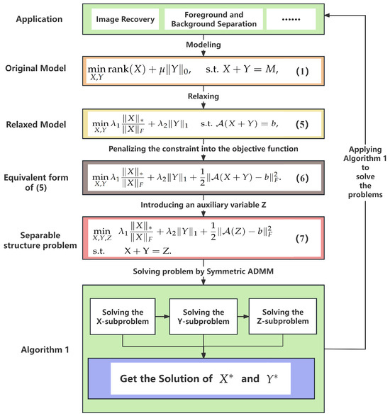
Figure 1. Summarized algorithm block diagram.

3. Convergence

This section mainly analyzes the convergence of the proposed algorithm. First, we provide the necessary definitions and concepts.

3.1. Preliminaries

For an extended-real-valued function g, the domain of g is defined as

$$\mathrm{dom}g:=\{\mathbf{x}\in {\mathbb{R}}^n|g\left(\mathbf{x}\right)<\infty \}.$$

A function g is closed if it is lower semicontinuous and is proper if $\mathrm{dom}g\ne \varnothing$ and $g\left(\mathbf{x}\right)>-\infty$ for any $\mathbf{x}\in \mathrm{dom}g$. For any point $\mathbf{x}\in {\mathbb{R}}^n$ and subset $S\subseteq {\mathbb{R}}^n$, the Euclidean distance from $\mathbf{x}$ to S is defined by

$$\mathrm{dist}(\mathbf{x},S):=inf\left\{\parallel \mathbf{y}-\mathbf{x}\parallel |\mathbf{y}\in S\right\},$$

where the notation $\parallel ·\parallel$ is ${\mathsf{\ell }}_2$ norm (calculated as the square root of the sum of squares of all vector entries). For a proper and closed function $g:{\mathbb{R}}^n\to \mathbb{R}\cup \{\infty \}$, a vector $\mathbf{u}\in \partial g\left(\mathbf{x}\right)$ is a subgradient of g at $\mathbf{x}\in \mathrm{dom}g$, where $\partial g$ denotes the subdifferential of g [29] defined by

$$\partial g\left(\mathbf{x}\right):=\left\{\mathbf{u}\in {\mathbb{R}}^n|\exists {\mathbf{x}}^k\to \mathbf{x},\widehat{\partial }g\left({\mathbf{x}}^k\right)\ni {\mathbf{u}}^k\to \mathbf{u}\mathrm{with}g\left({\mathbf{x}}^k\right)\to g\left(\mathbf{x}\right)\right\}$$

with $\widehat{\partial }g\left(\mathbf{x}\right)$ being the set of regular subgradients of g at $\mathbf{x}$:

$$\begin{array}{cc}\hfill \widehat{\partial }g\left(\mathbf{x}\right):=\{\mathbf{u}\in {\mathbb{R}}^n|g\left(\mathbf{y}\right)& \ge g\left(\mathbf{x}\right)+⟨\mathbf{u},\mathbf{y}-\mathbf{x}⟩+o(\parallel \mathbf{y}-\mathbf{x}\parallel )\forall \mathbf{y}\in {\mathbb{R}}^n\}.\hfill \end{array}$$

Note that if $f:{\mathbb{R}}^n\to \mathbb{R}$ is continuously differentiable and $g:{\mathbb{R}}^n\to \mathbb{R}\cup \{\infty \}$ is proper and lower semicontinuous, it follows from [29] that $\partial (f+g)=\nabla f+\partial g$. A point $x*$ is called a (limiting-) critical point or stationary point of F if it satisfies $0\in \partial F\left(\mathbf{x}*\right)$, and the set of critical points of F is denoted by $\mathrm{crit}F$.

Definition 1. 

We say that $(X*,Y*,Z*,\Lambda *)$ is a critical point of the augmented Lagrangian function ${\mathcal{L}}_{\beta }(·)$ if it satisfies

$$\left\{\begin{array}{c}0\in {\lambda }_1\partial \left({\displaystyle \frac{\parallel X*{\parallel }_{*}}{\parallel X*{\parallel }_F}}\right)+\Lambda *,\hfill \\ 0\in {\lambda }_2\partial (\parallel Y*{\parallel }_1)+\Lambda *,\hfill \\ 0={\mathcal{A}}^{\top }(\mathcal{A}\left(Z*\right)-b)-\Lambda *,\hfill \\ 0=X*+Y*-Z*.\hfill \end{array}\right.$$

It is evident that a critical point of the augmented Lagrange function ${\mathcal{L}}_{\beta }(·)$ is precisely the corresponding KKT point of (7). In this paper, we assume that there is at least one KKT point of (7).

3.2. Convergence

Next, we will analyze the convergence. Reviewing the iteration scheme (8a)–(8e), we next propose the following first-order optimality conditions for the subproblems in Algorithm 1.

Lemma 1. 

Let $\left\{(X^k,Y^k,Z^k,{\Lambda }^k)\right\}$ be the sequence generated by Algorithm 1. Then, we have

$$\left\{\begin{array}{c}0\in {\lambda }_1\partial \left({\displaystyle \frac{\parallel X^{k+1}{\parallel }_{*}}{\parallel X^{k+1}{\parallel }_F}}\right)+{\Lambda }^{k+1}+{\displaystyle \frac{\beta }{\alpha +1}}(Z^{k+1}-Z^k)-\beta (Y^{k+1}-Y^k)-{\displaystyle \frac{\alpha }{\alpha +1}}({\Lambda }^{k+1}-{\Lambda }^k),\hfill \\ 0\in {\lambda }_2\partial (\parallel Y^{k+1}{\parallel }_1)+{\Lambda }^{k+1}+{\displaystyle \frac{\beta }{\alpha +1}}(Z^{k+1}-Z^k)-{\displaystyle \frac{\alpha }{\alpha +1}}({\Lambda }^{k+1}-{\Lambda }^k),\hfill \\ 0={\mathcal{A}}^{\top }(\mathcal{A}\left(Z^{k+1}\right)-b)-{\Lambda }^{k+1},\hfill \\ {\Lambda }^{k+1}={\Lambda }^k+\beta [(\alpha +1)(X^{k+1}+Y^{k+1}-Z^k)-(Z^{k+1}-Z^k)].\hfill \end{array}\right.$$

(15)

Proof. 

Adding (8c) and (8e), we get

$$\begin{array}{cc}\hfill {\Lambda }^{k+1}-{\Lambda }^k& =\alpha \beta (X^{k+1}+Y^{k+1}-Z^k)+\beta (X^{k+1}+Y^{k+1}-Z^{k+1})\hfill \\ \hfill & =\alpha \beta (X^{k+1}+Y^k-Z^k)+\alpha \beta (Y^{k+1}-Y^k)\hfill \\ \hfill & +\beta (X^{k+1}+Y^k-Z^k)+\beta (Y^{k+1}-Y^k)-\beta (Z^{k+1}-Z^k)\hfill \\ \hfill & =(\alpha +1)\beta (X^{k+1}+Y^k-Z^k)+(\alpha +1)\beta (Y^{k+1}-Y^k)-\beta (Z^{k+1}-Z^k),\hfill \end{array}$$

and thus

$$X^{k+1}+Y^k-Z^k={\displaystyle \frac{1}{(\alpha +1)\beta }}({\Lambda }^{k+1}-{\Lambda }^k)-(Y^{k+1}-Y^k)+{\displaystyle \frac{1}{\alpha +1}}(Z^{k+1}-Z^k).$$

Based on the optimality condition of (8a),

$$\begin{array}{cc}\hfill 0& \in {\lambda }_1\partial \left({\displaystyle \frac{\parallel X^{k+1}{\parallel }_{*}}{\parallel X^{k+1}{\parallel }_F}}\right)+{\Lambda }^k+\beta (X^{k+1}+Y^k-Z^k)\hfill \\ \hfill & ={\lambda }_1\partial \left({\displaystyle \frac{\parallel X^{k+1}{\parallel }_{*}}{\parallel X^{k+1}{\parallel }_F}}\right)+{\Lambda }^{k+1}-({\Lambda }^{k+1}-{\Lambda }^k)+\beta (X^{k+1}+Y^k-Z^k)\hfill \\ \hfill & ={\lambda }_1\partial \left({\displaystyle \frac{\parallel X^{k+1}{\parallel }_{*}}{\parallel X^{k+1}{\parallel }_F}}\right)+{\Lambda }^{k+1}+{\displaystyle \frac{\beta }{\alpha +1}}(Z^{k+1}-Z^k)-\beta (Y^{k+1}-Y^k)-{\displaystyle \frac{\alpha }{\alpha +1}}({\Lambda }^{k+1}-{\Lambda }^k)\hfill \end{array}$$

Similarly,

$$\begin{array}{cc}\hfill {\Lambda }^{k+1}-{\Lambda }^k& =\alpha \beta (X^{k+1}+Y^{k+1}-Z^k)+\beta (X^{k+1}+Y^{k+1}-Z^{k+1})\hfill \\ \hfill & =(\alpha +1)\beta (X^{k+1}+Y^{k+1}-Z^k)-\beta (Z^{k+1}-Z^k).\hfill \end{array}$$

Therefore,

$$X^{k+1}+Y^{k+1}-Z^k={\displaystyle \frac{1}{(\alpha +1)\beta }}({\Lambda }^{k+1}-{\Lambda }^k)+{\displaystyle \frac{1}{\alpha +1}}(Z^{k+1}-Z^k).$$

(16)

By the optimality condition of (8b),

$$\begin{array}{cc}\hfill 0& \in {\lambda }_2\partial (\parallel Y^{k+1}{\parallel }_1)+{\Lambda }^k+\beta (X^{k+1}+Y^{k+1}-Z^k)\hfill \\ \hfill & ={\lambda }_2\partial (\parallel Y^{k+1}{\parallel }_1)+{\Lambda }^{k+1}-({\Lambda }^{k+1}-{\Lambda }^k)+\beta (X^{k+1}+Y^{k+1}-Z^k).\hfill \end{array}$$

Substituting (16) into the above inclusion yields, we get

$$0\in {\lambda }_2\partial (\parallel Y^{k+1}{\parallel }_1)+{\Lambda }^{k+1}+{\displaystyle \frac{\beta }{\alpha +1}}(Z^{k+1}-Z^k)-{\displaystyle \frac{\alpha }{\alpha +1}}({\Lambda }^{k+1}-{\Lambda }^k).$$

We also get the following equality by (8d)’s optimality condition,

$${\mathcal{A}}^{\top }(\mathcal{A}\left(Z^{k+1}\right)-b)-{\Lambda }^{k+{\displaystyle \frac{1}{2}}}-\beta (X^{k+1}+Y^{k+1}-Z^{k+1})=0.$$

And then from (8e),

$${\mathcal{A}}^{\top }(\mathcal{A}\left(Z^{k+1}\right)-b)-{\Lambda }^{k+1}=0.$$

(17)

In addition,

$$\begin{array}{cc}\hfill {\Lambda }^{k+1}& ={\Lambda }^{k+{\displaystyle \frac{1}{2}}}+\beta (X^{k+1}+Y^{k+1}-Z^{k+1})\hfill \\ \hfill & ={\Lambda }^k+\alpha \beta (X^{k+1}+Y^{k+1}-Z^k)+\beta (X^{k+1}+Y^{k+1}-Z^{k+1})\hfill \\ \hfill & ={\Lambda }^k+\beta [(\alpha +1)(X^{k+1}+Y^{k+1}-Z^k)-(Z^{k+1}-Z^k)].\hfill \end{array}$$

Therefore, (15) holds. This completes the proof. □

Lemma 2. 

Let $\{W^k:=(X^k,Y^k,Z^k,{\Lambda }^k)\}$ be the sequence generated by Algorithm 1. For any $\alpha \in (-1,1),\beta >{\displaystyle \frac{2}{1-\alpha }}L$ and $L={\sigma }_{max}\left({\mathcal{A}}^{\top }\mathcal{A}\right)$, we have the sequence $\left\{{\mathcal{L}}_{\beta }\left(W^k\right)\right\}$, which is decreasing, and

$${\mathcal{L}}_{\beta }\left(W^k\right)-{\mathcal{L}}_{\beta }\left(W^{k+1}\right)\ge c\parallel Z^{k+1}-Z^k{\parallel }_F^2+{\displaystyle \frac{\beta }{2}}{\parallel Y^{k+1}-Y^k|}_F^2,$$

where $c=\left({\displaystyle \frac{1}{\alpha +1}}-{\displaystyle \frac{1}{2}}\right)\beta -{\displaystyle \frac{L}{2}}-{\displaystyle \frac{L^2}{(\alpha +1)\beta }}>0$.

Proof. 

From (8a),

$$\begin{array}{cc}\hfill {\mathcal{L}}_{\beta }(X^k,Y^k,Z^k,{\Lambda }^k)-{\mathcal{L}}_{\beta }(X^{k+1},Y^k,Z^k,{\Lambda }^k)& \ge 0.\hfill \end{array}$$

(18)

Note that ${\mathcal{L}}_{\beta }(X^{k+1},Y,Z^k,{\Lambda }^k)$ is strongly convex and, with a modulus of at least $\beta$,

$$\begin{array}{cc}\hfill {\mathcal{L}}_{\beta }(X^{k+1},Y^k,Z^k,{\Lambda }^k)-{\mathcal{L}}_{\beta }(X^{k+1},Y^{k+1},Z^k,{\Lambda }^k)& \ge {\displaystyle \frac{\beta }{2}}{\parallel Y^{k+1}-Y^k\parallel }_F^2.\hfill \end{array}$$

(19)

$$\begin{array}{cc}\hfill & {\mathcal{L}}_{\beta }(X^{k+1},Y^{k+1},Z^k,{\Lambda }^{k+{\displaystyle \frac{1}{2}}})-{\mathcal{L}}_{\beta }(X^{k+1},Y^{k+1},Z^{k+1},{\Lambda }^{k+{\displaystyle \frac{1}{2}}})\hfill \\ \hfill =& {({\Lambda }^{k+{\displaystyle \frac{1}{2}}})}^{\top }(Z^{k+1}-Z^k)+{\displaystyle \frac{\beta }{2}}{\parallel X^{k+1}+Y^{k+1}-Z^k\parallel }_F^2\hfill \\ \hfill & +{\displaystyle \frac{1}{2}}\parallel \mathcal{A}\left(Z^k\right){-b\parallel }_F^2-{\displaystyle \frac{1}{2}}\parallel \mathcal{A}\left(Z^{k+1}\right){-b\parallel }_F^2-{\displaystyle \frac{\beta }{2}}{\parallel X^{k+1}+Y^{k+1}-Z^{k+1}\parallel }_F^2\hfill \\ \hfill =& {\displaystyle \frac{1}{2}}\parallel \mathcal{A}\left(Z^k\right){-b\parallel }_F^2-{\displaystyle \frac{1}{2}}{\parallel \mathcal{A}\left(Z^{k+1}\right)-b\parallel }_F^2\hfill \\ \hfill & -\beta {(X^{k+1}+Y^{k+1}-Z^k)}^{\top }(Z^{k+1}-Z^k)\hfill \\ \hfill & +{[{\Lambda }^k+(\alpha +1)\beta (X^{k+1}+Y^{k+1}-Z^k)]}^{\top }(Z^{k+1}-Z^k)\hfill \\ \hfill & +{\displaystyle \frac{\beta }{2}}\parallel X^{k+1}+Y^{k+1}-Z^k{\parallel }_F^2-{\displaystyle \frac{\beta }{2}}{\parallel X^{k+1}+Y^{k+1}-Z^{k+1}\parallel }_F^2\hfill \\ \hfill =& {\displaystyle \frac{1}{2}}\parallel \mathcal{A}\left(Z^k\right){-b\parallel }_F^2-{\displaystyle \frac{1}{2}}{\parallel \mathcal{A}\left(Z^{k+1}\right)-b\parallel }_F^2\hfill \\ \hfill & -{\displaystyle \frac{\beta }{2}}{\parallel Z^{k+1}-Z^k\parallel }_F^2+{[{\Lambda }^k+(\alpha +1)\beta (X^{k+1}+Y^{k+1}-Z^k)]}^{\top }(Z^{k+1}-Z^k)\hfill \\ \hfill =& {\displaystyle \frac{1}{2}}\parallel \mathcal{A}\left(Z^k\right){-b\parallel }_F^2-{\displaystyle \frac{1}{2}}{\parallel \mathcal{A}\left(Z^{k+1}\right)-b\parallel }_F^2\hfill \\ \hfill & -{\displaystyle \frac{\beta }{2}}{\parallel Z^{k+1}-Z^k\parallel }_F^2+{[{\Lambda }^k+({\Lambda }^{k+1}-{\Lambda }^k)+\beta (Z^{k+1}-Z^k)]}^{\top }(Z^{k+1}-Z^k)\hfill \\ \hfill =& {\displaystyle \frac{1}{2}}\parallel \mathcal{A}\left(Z^k\right){-b\parallel }_F^2-{\displaystyle \frac{1}{2}}\parallel \mathcal{A}\left(Z^{k+1}\right){-b\parallel }_F^2+{\left({\Lambda }^{k+1}\right)}^{\top }(Z^{k+1}-Z^k)+{\displaystyle \frac{\beta }{2}}{\parallel Z^{k+1}-Z^k\parallel }_F^2\hfill \\ \hfill \ge & {\displaystyle \frac{\beta -L}{2}}{\parallel Z^{k+1}-Z^k\parallel }_F^2,\hfill \end{array}$$

(20)

where the forth equality follows from (16), and the last inequality follows from [30], Lemma 1. Next, by using the definition of ${\mathcal{L}}_{\beta }(·)$ and (8c),

$$\begin{array}{cc}\hfill & {\mathcal{L}}_{\beta }(X^{k+1},Y^{k+1},Z^k,{\Lambda }^k)-{\mathcal{L}}_{\beta }(X^{k+1},Y^{k+1},Z^k,{\Lambda }^{k+{\displaystyle \frac{1}{2}}})\hfill \\ \hfill & +{\mathcal{L}}_{\beta }(X^{k+1},Y^{k+1},Z^{k+1},{\Lambda }^{k+{\displaystyle \frac{1}{2}}})-{\mathcal{L}}_{\beta }(X^{k+1},Y^{k+1},Z^{k+1},{\Lambda }^{k+1})\hfill \\ \hfill & ={({\Lambda }^k-{\Lambda }^{k+{\displaystyle \frac{1}{2}}})}^{\top }(X^{k+1}+Y^k-Z^k)+{({\Lambda }^{k+{\displaystyle \frac{1}{2}}}-{\Lambda }^{k+1})}^{\top }(X^{k+1}+Y^{k+1}-Z^{k+1})\hfill \\ \hfill & ={({\Lambda }^k-{\Lambda }^{k+1})}^{\top }(X^{k+1}+Y^{k+1}-Z^{k+1})-\alpha \beta {(X^{k+1}+Y^{k+1}-Z^k)}^{\top }(Z^{k+1}-Z^k)\hfill \end{array}$$

(21)

From (16),

$$\begin{array}{cc}\hfill X^{k+1}+Y^{k+1}-Z^{k+1}& =(X^{k+1}+Y^{k+1}-Z^k)-(Z^{k+1}-Z^k)\hfill \\ \hfill & ={\displaystyle \frac{1}{(\alpha +1)\beta }}({\Lambda }^{k+1}-{\Lambda }^k)+({\displaystyle \frac{1}{\alpha +1}}-1)(Z^{k+1}-Z^k)\hfill \\ \hfill & ={\displaystyle \frac{1}{(\alpha +1)\beta }}({\Lambda }^{k+1}-{\Lambda }^k)-{\displaystyle \frac{\alpha }{\alpha +1}}(Z^{k+1}-Z^k)\hfill \end{array}$$

(22)

Substituting (16) and (22) into (21),

$$\begin{array}{cc}\hfill & {\mathcal{L}}_{\beta }(X^{k+1},Y^{k+1},Z^k,{\Lambda }^k)-{\mathcal{L}}_{\beta }(X^{k+1},Y^{k+1},Z^k,{\Lambda }^{k+{\displaystyle \frac{1}{2}}})\hfill \\ \hfill & +{\mathcal{L}}_{\beta }(X^{k+1},Y^{k+1},Z^{k+1},{\Lambda }^{k+{\displaystyle \frac{1}{2}}})-{\mathcal{L}}_{\beta }(X^{k+1},Y^{k+1},Z^{k+1},{\Lambda }^{k+1})\hfill \\ \hfill & ={({\Lambda }^k-{\Lambda }^{k+1})}^{\top }\left[{\displaystyle \frac{{\Lambda }^{k+1}-{\Lambda }^k}{(\alpha +1)\beta }}-{\displaystyle \frac{\alpha }{\alpha +1}}(Z^{k+1}-Z^k)\right]\hfill \\ \hfill & -\alpha \beta {\left[{\displaystyle \frac{{\Lambda }^{k+1}-{\Lambda }^k}{(\alpha +1)\beta }}+{\displaystyle \frac{1}{\alpha +1}}(Z^{k+1}-Z^k)\right]}^{\top }(Z^{k+1}-Z^k)\hfill \\ \hfill & \ge -\left({\displaystyle \frac{L^2}{(\alpha +1)\beta }}+{\displaystyle \frac{\alpha \beta }{\alpha +1}}\right){\parallel Z^{k+1}-Z^k\parallel }_F^2,\hfill \end{array}$$

(23)

where the last inequality follows from (17) and $L={\sigma }_{max}\left({\mathcal{A}}^{\top }\mathcal{A}\right)$.

Summing (18)–(20), and (23),

$$\begin{array}{cc}\hfill {\mathcal{L}}_{\beta }\left(W^k\right)-{\mathcal{L}}_{\beta }\left(W^{k+1}\right)& \ge {\displaystyle \frac{\beta -L}{2}}{\parallel Z^{k+1}-Z^k\parallel }_F^2\hfill \\ \hfill & -\left[{\displaystyle \frac{L^2}{(\alpha +1)\beta }}+{\displaystyle \frac{\alpha \beta }{\alpha +1}}\right]\parallel Z^{k+1}-Z^k{\parallel }_F^2+{\displaystyle \frac{\beta }{2}}{\parallel Y^{k+1}-Y^k\parallel }_F^2\hfill \\ \hfill & ={\displaystyle \frac{\beta }{2}}{\parallel Y^{k+1}-Y^k\parallel }_F^2\hfill \\ \hfill & +\left[\left({\displaystyle \frac{1}{\alpha +1}}-{\displaystyle \frac{1}{2}}\right)\beta -{\displaystyle \frac{L}{2}}-{\displaystyle \frac{L^2}{(\alpha +1)\beta }}\right]{\parallel Z^{k+1}-Z^k\parallel }_F^2.\hfill \end{array}$$

If $\alpha \in (-1,1)$ and $\beta >{\displaystyle \frac{2}{1-\alpha }}L$ are given in Algorithm 1, we know that the sequence $\left\{{\mathcal{L}}_{\beta }\left(W^k\right)\right\}$ is decreasing. This completes the proof. □

Lemma 3. 

Let $\left\{W^k\right\}$ be the sequence generated by Algorithm 1. If $\left\{X^k\right\}$ is bounded, then for any $\alpha \in (-1,1),\beta >{\displaystyle \frac{2}{1-\alpha }}L$ and $L={\sigma }_{max}\left({\mathcal{A}}^{\top }\mathcal{A}\right)$, the whole sequence $\left\{W^k\right\}$ is bounded.

Proof. 

From Lemma 2,

$$\begin{array}{cc}\hfill & {\mathcal{L}}_{\beta }\left(W^1\right)\hfill \\ \hfill & \ge {\mathcal{L}}_{\beta }\left(W^k\right)\hfill \\ \hfill & ={\lambda }_1{\displaystyle \frac{\parallel X^k{\parallel }_{*}}{\parallel X^k{\parallel }_F}}+{\lambda }_2\parallel Y^k{\parallel }_1+{\displaystyle \frac{1}{2}}{\parallel \mathcal{A}\left(Z^k\right)-b\parallel }_F^2\hfill \\ \hfill & +⟨{\Lambda }^k,X^k+Y^k-Z^k⟩+{\displaystyle \frac{\beta }{2}}{\parallel X^k+Y^k-Z^k\parallel }_F^2\hfill \\ \hfill & ={\lambda }_1{\displaystyle \frac{\parallel X^k{\parallel }_{*}}{\parallel X^k{\parallel }_F}}+{\lambda }_2\parallel Y^k{\parallel }_1+{\displaystyle \frac{1}{2}}{\parallel \mathcal{A}\left(Z^k\right)-b\parallel }_F^2\hfill \\ \hfill & +⟨{\mathcal{A}}^{\top }(\mathcal{A}\left(Z^k\right)-b),X^k+Y^k-Z^k⟩+{\displaystyle \frac{\beta }{2}}{\parallel X^k+Y^k-Z^k\parallel }_F^2\hfill \\ \hfill & \ge {\lambda }_1{\displaystyle \frac{\parallel X^k{\parallel }_{*}}{\parallel X^k{\parallel }_F}}+{\lambda }_2\parallel Y^k{\parallel }_1+{\displaystyle \frac{1}{2}}\parallel \mathcal{A}(X^k+Y^k){-b\parallel }_F^2+{\displaystyle \frac{\beta -L}{2}}{\parallel X^k+Y^k-Z^k\parallel }_F^2\hfill \end{array}$$

(24)

where the second equality yields from (17) and the last inequality arises from [30], Lemma 1. Since $\alpha \in (-1,1),\beta >{\displaystyle \frac{2}{1-\alpha }}L$, we can easily see that $\beta >L$. By using the boundedness of $\left\{X^k\right\}$ and nonnegativity of the last inequality of (24), we find that $\left\{Y^k\right\}$, $\{X^k+Y^k\}$, and $\{X^k+Y^k-Z^k\}$ are bounded. According to the triangle inequality $\parallel Z^k{\parallel }_F\le \parallel X^k+Y^k{\parallel }_F+{\parallel X^k+Y^k-Z^k\parallel }_F$, we find that $\left\{Z^k\right\}$ is also bounded. In addition, from the boundedness of $\{\mathcal{A}(X^k+Y^k)-b\}$, we can derive that linear operator $\mathcal{A}$ is bounded. So, we have

$$\parallel {\Lambda }^k{\parallel }_F\le {\parallel {\mathcal{A}}^{\top }(\mathcal{A}\left(Z^k\right)-b)\parallel }_F,$$

which implies that $\left\{{\Lambda }^k\right\}$ is also bounded. Hence, $\left\{(X^k,Y^k,Z^k,{\Lambda }^k)\right\}$ is bounded. This completes the proof. □

Remark 1. 

The boundedness of $\left\{X^k\right\}$ is required throughout the subsequent analysis. In image processing, the elements in X represent pixel values ($[0,255]$), making the assumption of boundedness for X reasonable. Some studies [20,26,27] even directly constrain X within a specific box to replace the assumption of boundedness.

Lemma 4. 

Let $\left\{W^k\right\}$ be the sequence generated by Algorithm 1. If $\left\{X^k\right\}$ is bounded, then for any $\alpha \in (-1,1),\beta >{\displaystyle \frac{2}{1-\alpha }}L$ and $L={\sigma }_{max}\left({\mathcal{A}}^{\top }\mathcal{A}\right)$, there exists a positive constant m such that

$$\parallel \mathrm{dist}(0,\partial {\mathcal{L}}_{\beta }\left(W^{k+1}\right)){\parallel }_F^2\le m\left(\parallel Z^{k+1}-Z^k{\parallel }_F^2+{\parallel Y^{k+1}-Y^k\parallel }_F^2\right).$$

(25)

Proof. 

Define

$$\left\{\begin{array}{c}{w}_X^{k+1}:=({\Lambda }^{k+1}-{\Lambda }^k)+\beta (Y^{k+1}-Y^k)-\beta (Z^{k+1}-Z^k),\hfill \\ w_Y^{k+1}:=({\Lambda }^{k+1}-{\Lambda }^k)-\beta (Z^{k+1}-Z^k),\hfill \\ w_Z^{k+1}:=-{\displaystyle \frac{1}{\alpha +1}}({\Lambda }^{k+1}-{\Lambda }^k)+{\displaystyle \frac{\alpha \beta }{\alpha +1}}(Z^{k+1}-Z^k),\hfill \\ w_{\Lambda }^{k+1}:={\displaystyle \frac{1}{(\alpha +1)\beta }}({\Lambda }^{k+1}-{\Lambda }^k)-{\displaystyle \frac{\alpha }{\alpha +1}}(Z^{k+1}-Z^k).\hfill \end{array}\right.$$

From the definition of ${\mathcal{L}}_{\beta }(.)$,

$$\left\{\begin{array}{cc}\hfill {\partial }_X{\mathcal{L}}_{\beta }\left(W^{k+1}\right)& ={\lambda }_1\partial \left({\displaystyle \frac{\parallel X^{k+1}{\parallel }_{*}}{\parallel X^{k+1}{\parallel }_F}}\right)+{\Lambda }^{k+1}+\beta (X^{k+1}+Y^{k+1}-Z^{k+1}),\hfill \\ \hfill {\partial }_Y{\mathcal{L}}_{\beta }\left(W^{k+1}\right)& ={\lambda }_2\partial \left(\parallel Y^{k+1}{\parallel }_1\right)+{\Lambda }^{k+1}+\beta (X^{k+1}+Y^{k+1}-Z^{k+1}),\hfill \\ \hfill {\partial }_Z{\mathcal{L}}_{\beta }\left(W^{k+1}\right)& ={\mathcal{A}}^{\top }(\mathcal{A}\left(Z^{k+1}\right)-b)-{\Lambda }^{k+1}-\beta (X^{k+1}+Y^{k+1}-Z^{k+1}),\hfill \\ \hfill {\partial }_{\Lambda }{\mathcal{L}}_{\beta }\left(W^{k+1}\right)& =X^{k+1}+Y^{k+1}-Z^{k+1}.\hfill \end{array}\right.$$

Then, it follows from (15) and (22) that $(w_X^{k+1},w_Y^{k+1},w_Z^{k+1},w_{\Lambda }^{k+1})\in \partial {\mathcal{L}}_{\beta }\left(W^{k+1}\right)$.

$$\begin{array}{cc}\hfill \parallel (w_X^{k+1},w_Y^{k+1},w_Z^{k+1},w_{\Lambda }^{k+1}){\parallel }_F^2& \le \parallel w_X^{k+1}{\parallel }_F^2+\parallel w_Y^{k+1}{\parallel }_F^2+\parallel w_Z^{k+1}{\parallel }_F^2+{\parallel w_{\Lambda }^{k+1}\parallel }_F^2\hfill \\ \hfill & \le 4{\beta }^2{\parallel Y^{k+1}-Y^k\parallel }_F^2\hfill \\ \hfill & +\left(6+{\displaystyle \frac{2}{{(\alpha +1)}^2}}+{\displaystyle \frac{2}{{(\alpha +1)}^2{\beta }^2}}\right){\parallel {\Lambda }^{k+1}-{\Lambda }^k\parallel }_F^2\hfill \\ \hfill & +\left(2{\beta }^2+{\displaystyle \frac{2{\alpha }^2{\beta }^2}{{(\alpha +1)}^2}}+{\displaystyle \frac{2{\alpha }^2}{{(\alpha +1)}^2}}\right){\parallel Z^{k+1}-Z^k\parallel }_F^2\hfill \end{array}$$

Again, from (17), we set

$$m:=max\left\{\left(6+{\displaystyle \frac{2}{{(\alpha +1)}^2}}+{\displaystyle \frac{2}{{(\alpha +1)}^2{\beta }^2}}\right)L^2+2{\beta }^2+{\displaystyle \frac{2{\alpha }^2{\beta }^2}{{(\alpha +1)}^2}}+{\displaystyle \frac{2{\alpha }^2}{{(\alpha +1)}^2}},4{\beta }^2\right\},$$

which implies that (25) holds. This completes the proof. □

Lemma 5. 

Let $\left\{W^k\right\}$ be the sequence generated by Algorithm 1. If $\left\{X^k\right\}$ is bounded, then for any $\alpha \in (-1,1),\beta >{\displaystyle \frac{2}{1-\alpha }}L$ and $L={\sigma }_{max}\left({\mathcal{A}}^{\top }\mathcal{A}\right)$, we have

$$\underset{k\to \infty }{lim}(\parallel X^{k+1}-X^k{\parallel }_F+\parallel Y^{k+1}-Y^k{\parallel }_F+\parallel Z^{k+1}-Z^k{\parallel }_F+\parallel {\Lambda }^{k+1}-{\Lambda }^k{\parallel }_F)=0.$$

Proof. 

From the result of Lemma 2,

$${\mathcal{L}}_{\beta }\left(W^{k+1}\right)\le {\mathcal{L}}_{\beta }\left(W^1\right)-c\sum _{j=1}^k\parallel Z^{j+1}-Z^j{\parallel }_F^2-{\displaystyle \frac{\beta }{2}}\sum _{j=1}^k{\parallel Y^{j+1}-Y^j\parallel }_F^2.$$

From (24), we have ${\mathcal{L}}_{\beta }\left(W^{k+1}\right)\ge 0$. Let $k\to \infty$. We know that ${\sum }_{j=1}^{\infty }{\parallel Z^{j+1}-Z^j\parallel }_F^2<\infty$ and ${\sum }_{j=1}^{\infty }{\parallel Y^{j+1}-Y^j\parallel }_F^2<\infty$ which implies that

$$\underset{k\to \infty }{lim}\parallel Z^{k+1}-Z^k{\parallel }_F=0\mathrm{and}\underset{k\to \infty }{lim}{\parallel Y^{k+1}-Y^k\parallel }_F=0.$$

According to (17), we have $\underset{k\to \infty }{lim}{\parallel {\Lambda }^{k+1}-{\Lambda }^k\parallel }_F=0.$ Moreover, from (22), we have $\underset{k\to \infty }{lim}{\parallel X^{k+1}-X^k\parallel }_F=0.$ This completes the proof. □

By utilizing the Kurdyka–Lojasiewicz (KL) property [30,31] and previous conclusions, we can ensure the convergence of the generated sequence to a critical point. In the following theorems, we summarize these results, and the proof process is similar to the proof techniques in references [28,30,31,32,33,34,35]. Due to the limited space, the specific proof steps are omitted here.

Theorem 1. 

Let $\left\{W^k\right\}$ be the sequence generated by Algorithm 1 and $\alpha \in (-1,1),\beta >{\displaystyle \frac{2}{1-\alpha }}L$, $L={\sigma }_{max}\left({\mathcal{A}}^{\top }\mathcal{A}\right)$. If $\left\{X^k\right\}$ is bounded, then any cluster point $W*:=(X*,Y*,Z*,\Lambda *)$ of the sequence $\left\{W^k\right\}$ is a critical point of (7).

Theorem 2. 

Let $\left\{W^k\right\}$ be the sequence generated by Algorithm 1. If $\beta >{\displaystyle \frac{2}{1-\alpha }}L$, $\alpha \in (-1,1)$, $L={\sigma }_{max}\left({\mathcal{A}}^{\top }\mathcal{A}\right)$, and $\left\{X^k\right\}$ is bounded, then $\left\{W^k\right\}$ has finite length, i.e.,

$$\sum _{k=1}^{\infty }{\parallel W^{k+1}-W^k\parallel }_F^2<\infty ,$$

and hence $\left\{W^k\right\}$ globally converges to the critical point of (7).

4. Numerical Results

We apply the proposed SADMM to principal component analysis experiments on synthetic data, image recovery, and background and foreground separations of surveillance videos to validate its effectiveness. For these experiments, we focus on addressing the following RPCA problem:

$$\begin{array}{cc}\hfill & \underset{X,Y,Z}{min}{\lambda }_1{\displaystyle \frac{{\parallel X\parallel }_{*}}{{\parallel X\parallel }_F}}+{\lambda }_2{\parallel Y\parallel }_1+{\displaystyle \frac{1}{2}}{\parallel P_{\mathrm{\Omega }}\left(Z\right)-P_{\mathrm{\Omega }}\left(M\right)\parallel }_F^2\hfill \\ \hfill & \mathrm{s}.\mathrm{t}.\mathrm{X}+\mathrm{Y}=\mathrm{Z}.\hfill \end{array}$$

All codes were written and run using MATLAB 2021a software on a Windows 10 laptop equipped with an Intel(R) Core(TM) i7-1165G7 processor, a 2.80 GHz clock speed, and 16 GB of RAM. All the numerical results are the averages of 10 random running trials.

4.1. Synthetic Data

The purpose of this subsection is to compare the numerical performance of the classical ADMM ($\alpha =0$) and the proposed SADMM under the same experimental conditions. We mainly tested the effect of different values of $\alpha \in (-1,1)$ on the numerical results.

Let $M=X+Y$ be the observed matrix, where X and Y represent the low-rank and sparse components to be recovered, respectively. The dimension of M is $m\times n$. We generate rank-r matrix X via $X=M_L{M}_R$, where $M_L\in {\mathcal{R}}^{m\times r}$ and $M_R\in {\mathcal{R}}^{r\times n}$ are randomly generated using the MATLAB 2021a $\mathbf{command}\mathbf{rand}$. The low rank of X is controlled by $rr$ (i.e., $rr=r/m$), the sparsity of Y is controlled by $spr$ ( i.e., ${\parallel Y\parallel }_0/mn$ ), $sr$ is the ratio of sample (observed) entries (i.e., $\left|\mathrm{\Omega }\right|/mn$), and $\left|\mathrm{\Omega }\right|$ is the cardinality of $\mathrm{\Omega }$). Based on the $spr$, we randomly selected non-zero positions and set the elements at them to random numbers within the range $[-500,500]$ to construct the sparse matrix Y. We started process with the initial iteration values $(X^0,Y^0,Z^0)=(\mathbf{0},\mathbf{0},\mathbf{0})$. We set the experimental parameters as $m=n=300$, ${\lambda }_1=100$, ${\lambda }_2=10$, $\beta =\delta =0.05$, and $rr=spr=0.05$, $sr=0.9$, and the maximum iteration numbers $k_{max}$ and $t_{max}$ for the outer and inner iterations, respectively, as 500 and 5. The stopping criterion $Tol$ is set to ${10}^{-5}$ in this subsection.

Table 2 presents CPU time (Time), the iteration number (Iter.), and relative error (RE:=$\parallel X*{-X\parallel }_F/{\parallel X\parallel }_F$, where $X*$ is the recovered matrix) for different values of $\alpha$. The numerical results reveals that $\alpha =0.5$ delivers the optimal performance while maintaining a relatively stable relative error.

Table 2. The iteration time and number of iterations corresponding to different $\alpha$ values.

$\mathit{\alpha }$	−0.5	−0.3	0	0.3	0.5	0.7	0.9
Time	9.61	7.63	6.05	4.88	4.38	5.31	10.63
Iter.	156	114	85	71	63	77	154
RE	$3.70\times {10}^{-3}$	$3.40\times {10}^{-3}$	$2.70\times {10}^{-3}$	$2.10\times {10}^{-3}$	$2.02\times {10}^{-3}$	$9.38\times {10}^{-3}$	$1.81\times {10}^{-3}$

We further investigated the convergence properties of the SADMM. Figure 2 shows the evolution of the relative error and the rank of low-rank matrix X as the number of iterations increases, for parameters $\alpha =-0.5,0,0.5,0.9$, respectively. Observing the left side of Figure 2, it is evident that when $\alpha =0.5$, the SADMM exhibits a faster convergence rate compared to the traditional ADMM. From the right side of Figure 2, we can conclude that, during the initial few iterations, the rank changes caused by $\alpha =0.5$ are more pronounced than $\alpha =0$; however, $\alpha =0.5$ can more quickly reach the true low-rank state, and the low-rank characteristics remain stable throughout the iteration process.

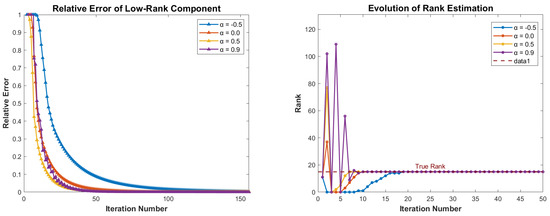
Figure 2. Evolutions of the relative error of low-rank (left) and rank estimation (right) for $\alpha =-0.5$, $\alpha =0$, $\alpha =0.5$, and $\alpha =0.9$.

Based on the above results, it can be observed that the SADMM achieves the most optimal performance when $\alpha =0.5$. To further evaluate the advantage of the proposed model, we solve it with the SADMM with the parameter $\alpha$ set to $0.5$ (the optimal parameter) and apply it to the subsequent image processing and video surveillance experiments.

4.2. Image Recovery

In this subsection, we mainly evaluate the effectiveness of the SADMM through the recovery of real images. In practical applications, the original image is often not low-rank, but its essential information is often dominated by high singular values. Therefore, we can approximately regard it as a low-rank matrix. The observed original image is often damaged or obscured, resulting in the loss of some elements. That is, the observed matrix M can be approximately regarded as the sum of the low-rank matrix X and the sparse noise matrix Y. Therefore, the purpose of this subsection is to recover the low-rank part from the partially damaged image, which is the matrix completion problem. We compare the SADMM with three other classical algorithms used for matrix completion problems. They are the Accelerated Iteratively Reweighted Nuclear Norm algorithm (AIRNN) [36], Singular Value Thresholding algorithm (SVT) [37], and the Schatten Capped p norm minimization method (SC_p) [16]. In this experiment, the parameters in the SADMM were set as ${\lambda }_1=50$, ${\lambda }_2=5$, $\beta =0.5$, $\delta =0.05$, and $k_{max}=120$, $t_{max}=5$. The parameters in AIRNN, SVT, and SC_p were all set to the optimal parameters used in the corresponding literature, and $Tol={10}^{-5}$.

Figure 3 presents four image samples captured by our team, including four color images: “Tower ($256\times 256$)”, “Sky ($512\times 512$)”, “Spillikins ($512\times 512$)” and “Texture ($512\times 512$)”. We simulated partial image damage by randomly removing $50\%$ of the real data (for color images, each channel was processed separately and then averaged). Figure 3 also shows the performance of different algorithms in recovering damaged images.

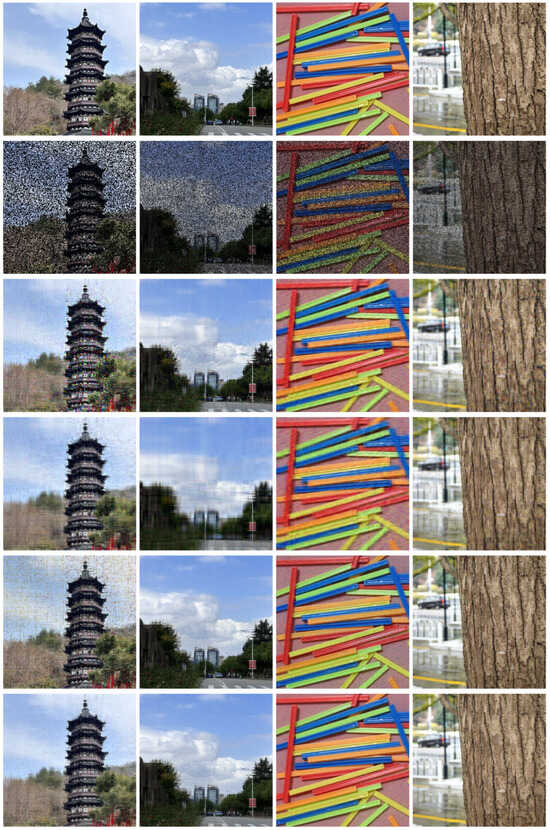
Figure 3. Image restoration results under 50% random pixel loss using different methods. Scene contains Tower, Sky, Spillikins, and Texture. From top to bottom: Original, Damaged, AIRNN, SVT, SC_p, SADMM.

In order to further evaluate the performance of the SADMM and the proposed model, Table 3 lists the numerical results of the four algorithms, AIRNN, SVT, SC_p, and SADMM, including the Signal-to-Noise Ratio (SNR) and relative error (RE) between the original image X and the recovered image $X*$. The SNR was calculated with the following formula:

$$\mathrm{SNR}:=10{log}_{10}{\displaystyle \frac{\parallel X-\overline{X}{\parallel }^2}{\parallel X-X*{\parallel }^2}}$$

where $\overline{X}$ is the mean of the original data.

Table 3. Numerical results of different algorithms on various images.

Images	AIRNN		SVT		SCp		SADMM
	SNR	RE	SNR	RE	SNR	RE	SNR	RE
Tower	16.50	0.1915	21.98	0.1318	13.33	0.2003	23.13	0.1084
Sky	25.97	0.1083	23.94	0.1200	29.32	0.0831	30.70	0.0770
Spillikins	18.16	0.1129	16.21	0.1402	19.61	0.1024	25.13	0.0649
Texture	19.19	0.1943	18.74	0.1978	19.94	0.1677	20.62	0.1462
Average	19.95	0.1517	20.21	0.1474	20.55	0.1383	24.89	0.0991

The numerical results in Table 3 show that the SADMM demonstrated better recovery performance when solving the proposed model. Figure 4 further shows the evolution tendency of the SNR values of the four methods as the number of iterations increased. From Figure 4, it can be observed that, under the same number of iterations, the proposed SADMM achieved better image recovery results than the other three algorithms.

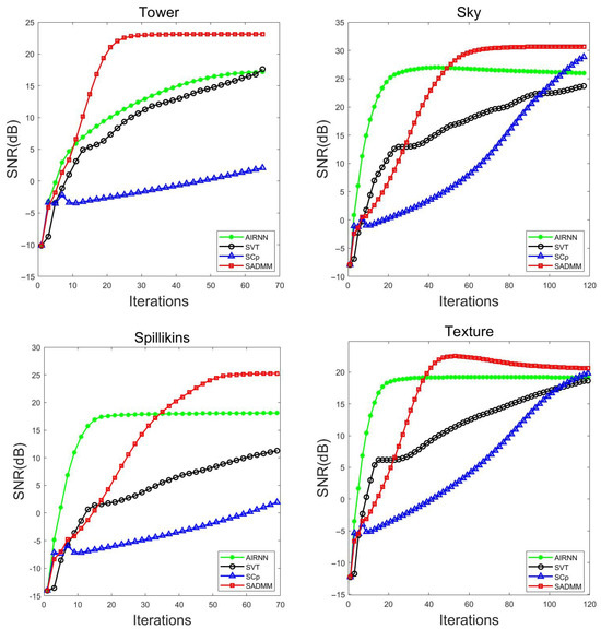
Figure 4. Evolution of SNR values as the number of iterations increases.

4.3. Foreground and Background Separation in Surveillance Video

In this subsection, We apply the proposed algorithm to the problem of separating the foreground and background in surveillance video, which is a typical RPCA problem. We test the algorithm using two surveillance video datasets: restaurant and shopping mall surveillance videos. They can be obtained from https://hqcai.org/datasets/restaurant.mat (accessed on 13 July 2025) and https://hqcai.org/datasets/shoppingmall.mat (accessed on 13 July 2025) of [38]. The details of these videos, including the resolution and the number of frames, are shown in Table 4, where each column of the matrix corresponds to a frame of the video. The index set $\mathrm{\Omega }$ of missing information is randomly determined based on the specified sample ratio $sr$. In the following experiment, we set $sr=0.9$, which means that $10\%$ of the information in the test video was randomly removed.

Table 4. Dataset description. The video name, resolution, and the number of frames.

Video Name	Resolution	The Number of Frames
Restaurant	$120\times 160$	200
Shopping Mall	$256\times 320$	400

In order to further evaluate algorithm performance and model accuracy, we compare the parallel split augmented Lagrange method from [39] with the Optimal Proximal Augmented Lagrange Method (OPALM) from [40]. For clarity, the dynamic step size and constant step size strategies used in [39] are labeled Alg1d and Alg1c, respectively. The parameter settings of the SADMM are ${\lambda }_1=1$, ${\lambda }_2=1/\sqrt{m}$, $\beta =0.004/{\parallel M\parallel }_1$, $\delta =0.05$, $k_{max}=100$, and $t_{max}=5$, respectively. The relevant parameter settings of Alg1d, Alg1c, and OPALM are the same as those in the corresponding literature, with the stopping criteria $Tol=3\times {10}^{-2}$.

Figure 5 shows the original frames and the corrupted frames of the 150th and 200th frames in the restaurant surveillance video and the 350th and 400th frames in the shopping mall surveillance video.

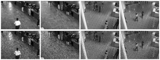
Figure 5. The 150th and 200th frames in the restaurant surveillance video and the 350th and 400th frames in the shopping mall surveillance video, showing the original frames (top row) and the corrupted frames (bottom row).

Figure 6 shows the results of different algorithms separating the foreground and background images from a video sequence. The images displayed in Figure 6 are selected from the 150th and 200th frames of the restaurant video and the 350th and 400th frames of the shopping mall video. Table 5 provides a detailed list of the rank of the low-rank matrix (denoted as rank($X*$)), the sparsity of the sparse matrix (denoted as $\parallel Y*{\parallel }_0$), and the relative error (denoted as ${\displaystyle \frac{\parallel M-X*-Y*{\parallel }_F}{{\parallel M\parallel }_F}}$) for the reconstructed matrices using different methods. According to the data presented in Table 5, it can be observed that, at the end of the iteration process, the ranks of the low-rank matrices obtained by each algorithm remain consistent, and the differences in the sparsity of sparse matrices are minimal. In addition, the SADMM demonstrated smaller relative errors across the two datasets, further indicating that the fractional regularization model proposed in this paper achieves higher accuracy.

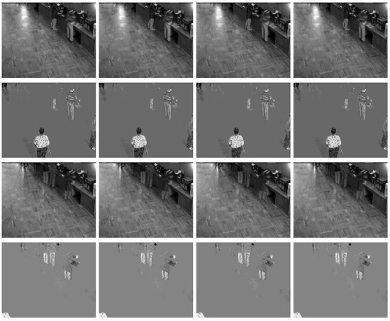
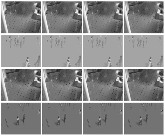
Figure 6. Foreground and background separation in surveillance videos separated by the tested algorithms. Columns 1–4 correspond to the results of the Alg1d, Alg1c, OPALM, and SADMM, respectively. From top to bottom: the 150th and 200th frames of the restaurant video and the 350th and 400th frames of the shopping mall video.

Table 5. Numerical results for background extraction on surveillance videos.

Method	Rank($X*$)		$\parallel Y*{\parallel }_0$		$\frac{\parallel M-X*-Y*{\parallel }_F}{{\parallel M\parallel }_F}$
	Restaurant	Shopping Mall	Restaurant	Shopping Mall	Restaurant	Shopping Mall
Alg1d	18	20	551,326	2,698,367	$8.11\times {10}^{-2}$	$3.68\times {10}^{-2}$
Alg1c	18	20	548,238	2,804,602	$8.16\times {10}^{-2}$	$3.69\times {10}^{-2}$
OPALM	18	20	526,557	2,795,618	$8.22\times {10}^{-2}$	$3.71\times {10}^{-2}$
SADMM	18	20	561,197	2,818,965	$8.10\times {10}^{-2}$	$3.66\times {10}^{-2}$

5. Conclusions

This paper proposes a nonconvex fractional regularization model to address the rank approximation problem in robust principal component analysis. A more general symmetric alternating direction method of multipliers is employed to solve it, and the convergence is proved. The final results also validate the effectiveness of our algorithm. However, the iterative solution of the X subproblem imposes certain limitations on the scalability of this algorithm. Future work will explore explicit solutions for subproblem X and test the model on larger-scale real-world datasets.

References

- Candès, E.J.; Li, X.D.; Ma, Y.; Wright, J. Robust principal component analysis? J. ACM 2011, 58, 11. [Google Scholar] [CrossRef]
- Huang, Y.; Wang, Z.; Chen, Q.; Chen, W. Robust principal component analysis via truncated L1−2 minimization. In Proceedings of the 2023 International Joint Conference on Neural Networks, Gold Coast, Australia, 18–23 June 2023; pp. 1–9. [Google Scholar] [CrossRef]
- Bian, J.T.; Zhao, D.D.; Nie, F.P.; Wang, R.; Li, X.L. Robust and sparse principal component analysis with adaptive loss minimization for feature selection. IEEE T. Neur. Net. Lear. 2022, 35, 3601–3614. [Google Scholar] [CrossRef] [PubMed]
- Wang, Q.S.; Han, D.R.; Zhang, W.X. A customized inertial proximal alternating minimization for SVD-free robust principal component analysis. Optimization 2023, 73, 2387–2412. [Google Scholar] [CrossRef]
- Shen, Y.; Xu, H.Y.; Liu, X. An alternating minimization method for robust principal component analysis. Optim. Method Softw. 2018, 34, 1251–1276. [Google Scholar] [CrossRef]
- Zhuang, S.T.; Wang, Q.W.; Chen, J.F. Dual graph Laplacian RPCA method for face recognition based on anchor points. Symmetry 2025, 17, 691. [Google Scholar] [CrossRef]
- Zhang, W.T.; Chen, X.H. Robust discriminative non-negative and symmetric low-rank projection learning for feature extraction. Symmetry 2025, 17, 307. [Google Scholar] [CrossRef]
- Wright, J.; Peng, Y.G.; Ma, Y.; Ganesh, A.; Rao, S. Robust principal component analysis: Exact recovery of corrupted low-rank matrices via convex optimization. In Proceedings of the 23rd International Conference on Neural Information Processing Systems, Vancouver, BC, Canada, 7–10 December 2009; pp. 2080–2088. Available online: https://dl.acm.org/doi/abs/10.5555/2984093.2984326 (accessed on 13 July 2025).
- Tao, M.; Yuan, X.M. Recovering low-rank and sparse components of matrices from incomplete and noisy observations. SIAM J. Optim. 2011, 21, 57–81. [Google Scholar] [CrossRef]
- Fan, J.Q.; Li, R.Z. Variable selection via nonconcave penalized likelihood and its oracle properties. J. Am. Stat. Assoc. 2001, 96, 1348–1360. [Google Scholar] [CrossRef]
- Zhang, C.H. Nearly unbiased variable selection under minimax concave penalty. Ann. Stat. 2010, 38, 894–942. [Google Scholar] [CrossRef] [PubMed]
- Zhang, T. Analysis of multi-stage convex relaxation for sparse regularization. J. Mach. Learn. Res. 2010, 11, 1081–1107. Available online: https://dl.acm.org/doi/10.5555/1756006.1756041 (accessed on 13 July 2025).
- Candès, E.J.; Wakin, M.B.; Boyd, S.P. Enhancing sparsity by reweighted ℓ1 minimization. J. Fourier Anal. Appl. 2008, 14, 877–905. [Google Scholar] [CrossRef]
- Friedman, J.H. Fast sparse regression and classification. Int. J. Forecasting 2012, 28, 722–738. [Google Scholar] [CrossRef]
- Nie, F.P.; Huang, H.; Ding, C. Low-rank matrix recovery via efficient schatten p-norm minimization. In Proceedings of the 26-th AAAI Conference on Artificial Intelligence, Toronto, ON, Canada, 22–26 July 2012; pp. 655–661. Available online: https://dl.acm.org/doi/10.5555/2900728.2900822 (accessed on 13 July 2025).
- Li, X.L.; Zhang, H.Y.; Zhang, R. Matrix completion via non-convex relaxation and adaptive correlation learning. IEEE Trans. Pattern Anal. Mach. Intell. 2023, 45, 1981–1991. [Google Scholar] [CrossRef] [PubMed]
- Gao, C.X.; Wang, N.Y.; Yu, Q.; Zhang, Z.H. A feasible nonconvex relaxation approach to feature selection. In Proceedings of the 25th AAAI Conference on Artificial Intelligence, San Francisco, CA, USA, 7–11 August 2011; pp. 356–361. [Google Scholar] [CrossRef]
- Geman, D.; Yang, C.D. Nonlinear image recovery with half-quadratic regularization. IEEE T. Image Process. 1995, 4, 932–946. [Google Scholar] [CrossRef] [PubMed]
- Trzasko, J.; Manduca, A. Highly undersampled magnetic resonance image reconstruction via homotopy ℓ0-minimization. IEEE T. Med. Imaging 2009, 28, 106–121. [Google Scholar] [CrossRef]
- Gao, K.X.; Huang, Z.H.; Guo, L.L. Low-rank matrix recovery problem minimizing a new ratio of two norms approximating the rank function then using an ADMM-type solver with applications. J. Comput. Appl. Math. 2024, 438, 115564. [Google Scholar] [CrossRef]
- Rahimi, Y.; Wang, C.; Dong, H.B.; Lou, Y.F. A scale-invariant approach for sparse signal recovery. SIAM J. Sci. Comput. 2019, 41, A3649–A3672. [Google Scholar] [CrossRef]
- Wang, C.; Yan, M.; Rahimi, Y.; Lou, Y.F. Accelerated schemes for the L1/L2 minimization. IEEE Trans. Signal Process. 2020, 68, 2660–2669. [Google Scholar] [CrossRef]
- Tao, M. Minimization of L1 over L2 for sparse signal recovery with convergence guarantee. SIAM J. Sci. Comput. 2022, 44, A770–A797. [Google Scholar] [CrossRef]
- Hurley, N.; Rickard, S. Comparing measures of sparsity. IEEE T. Inform. Theory 2009, 55, 4723–4741. [Google Scholar] [CrossRef]
- Yin, P.H.; Esser, E.; Xin, J. Ratio and difference of l1 and l2 norms and sparse representation with coherent dictionaries. Commun. Inf. Syst. 2014, 14, 87–109. [Google Scholar] [CrossRef]
- Wang, C.; Tao, M.; Nagy, J.G.; Lou, Y.F. Limited-angle CT reconstruction via the L1/L2 minimization. SIAM J. Imaging Sci. 2021, 14, 749–777. [Google Scholar] [CrossRef]
- Wang, C.; Tao, M.; Chuah, C.N.; Nagy, J.G.; Lou, Y.F. Minimizing L1 over L2 norms on the gradient. Inverse Probl. 2022, 38, 065011. [Google Scholar] [CrossRef]
- Wu, Z.M.; Li, M.; Wang, D.Z.W.; Han, D.R. A symmetric alternating direction method of multipliers for separable nonconvex minimization problems. Asia. Pac. J. Oper. Res. 2017, 34, 1750030. [Google Scholar] [CrossRef]
- Rockafellar, R.T.; Wets, R.J.B. Variational Analysis; Springer: Berlin/Heidelberg, Germany, 2009. [Google Scholar] [CrossRef]
- Bolte, J.; Sabach, S.; Teboulle, M. Proximal alternating linearized minimization for nonconvex and nonsmooth problems. Math. Program. 2014, 146, 459–494. [Google Scholar] [CrossRef]
- Attouch, H.; Bolte, J.; Svaiter, B.F. Convergence of descent methods for semi-algebraic and tame problems: Proximal algorithms, forward−backward splitting, and regularized Gauss−Seidel methods. Math. Program. 2013, 137, 91–129. [Google Scholar] [CrossRef]
- Guo, K.; Han, D.R.; Wu, T.T. Convergence of alternating direction method for minimizing sum of two nonconvex functions with linear constraints. Int. J. Comput. Math. 2016, 94, 1653–1669. [Google Scholar] [CrossRef]
- Ge, Z.L.; Zhang, X.; Wu, Z.M. A fast proximal iteratively reweighted nuclear norm algorithm for nonconvex low-rank matrix minimization problems. Appl. Numer. Math. 2022, 179, 66–86. [Google Scholar] [CrossRef]
- Ge, Z.L.; Wu, Z.M.; Zhang, X.; Ni, Q. An extrapolated proximal iteratively reweighted method for nonconvex composite optimization problems. J. Glob. Optim. 2023, 86, 821–844. [Google Scholar] [CrossRef]
- Ge, Z.L.; Zhang, S.Y.; Zhang, X.; Cui, Y. A new proximal iteratively reweighted nuclear norm method for nonconvex nonsmooth optimization problems. Mathematics 2025, 13, 2630. [Google Scholar] [CrossRef]
- Phan, D.N.; Nguyen, T.N. An accelerated IRNN-Iteratively Reweighted Nuclear Norm algorithm for nonconvex nonsmooth low-rank minimization problems. J. Comput. Appl. Math. 2021, 396, 113602. [Google Scholar] [CrossRef]
- Cai, J.F.; Candès, E.J.; Shen, Z.W. A singular value thresholding algorithm for matrix completion. SIAM J. Optim. 2010, 20, 1956–1982. [Google Scholar] [CrossRef]
- Giampouras, P.; Cai, H.Q.; Vidal, R. Guarantees of a preconditioned subgradient algorithm for overparameterized asymmetric low-rank matrix recovery. arXiv 2025, arXiv:2410.16826. [Google Scholar] [CrossRef]
- Jiang, F.; Lu, B.Y.; Wu, Z.M. Revisiting parallel splitting augmented Lagrangian method: Tight convergence and ergodic convergence rate. CSIAM T. Appl. Math. 2024, 5, 884–913. [Google Scholar] [CrossRef]
- He, B.S.; Ma, F.; Yuan, X.M. Optimal proximal augmented Lagrangian method and its application to full Jacobian splitting for multi-block separable convex minimization problems. IMA J. Numer. Anal. 2020, 40, 1188–1216. [Google Scholar] [CrossRef]
Disclaimer/Publisher’s Note: The statements, opinions and data contained in all publications are solely those of the individual author(s) and contributor(s) and not of MDPI and/or the editor(s). MDPI and/or the editor(s) disclaim responsibility for any injury to people or property resulting from any ideas, methods, instructions or products referred to in the content. |
© 2025 by the authors. Licensee MDPI, Basel, Switzerland. This article is an open access article distributed under the terms and conditions of the Creative Commons Attribution (CC BY) license (https://creativecommons.org/licenses/by/4.0/).