Abstract
This study employs Markov-Switching Regression (MS-Regression) to model four macroeconomic indicators—US GDP, CPI, interest rate, and unemployment rate—to identify economic crisis cycles, while all indicators provide some level of insight into these cycles, the unemployment rate offers the closest alignment with the actual patterns of economic cycles. Based on the regime identification derived from the unemployment rate, we delineate the time series for expansion and recession periods. Subsequently, we apply the Quantile Vector Autoregression (Quantile-VAR) model to analyze three sets of time series: the entire dataset, the expansion period, and the recession period. Our findings reveal that, under normal conditions, the US dollar exerts the greatest influence on and is most influenced by other currencies, whereas the Australian dollar has the least impact on others. In the extreme lower and upper tails, the mutual influence among the currencies of different countries intensifies, concurrently diminishing the relative influence of the US dollar. Notably, the spillover effects under extreme lower and upper tail conditions are not consistent, as the occurrence of extreme values does not coincide, suggesting an asymmetry in the spillover effects at these quantiles.
1. Introduction
The exchange market plays a crucial role in global financial systems, acting as a primary asset class that continuously attracts market participants from around the world. Over time, an increasing body of research has highlighted the interconnections and interdependencies that exist between various currencies in the exchange market. These studies consistently demonstrate that currency shocks originating from specific economies are not isolated phenomena but tend to propagate across other currencies [1]. Ref. [2] confirms the interdependence among currencies by calculating the spillover effects of volatility among seven major currencies. Ref. [3] utilizes the Gumbel Copula model to confirm the existence of long-run causal links and significant bidirectional causality among the exchange rates of various countries. In particular, the co-movement of the exchange rates among the ASEAN-5 countries significantly increased during the global financial crisis [4]. Such interdependencies in the exchange market have significant implications for international trade, risk management, and portfolio diversification. Moreover, understanding these connections is critical for policymakers because the behavior of one currency affects others, complicating the task of controlling the value of a currency through domestic monetary policy alone. This presents a huge challenge for monetary authorities, especially in a highly interconnected global market.
While the interdependency of currencies in the exchange market is widely acknowledged, the strength and nature of these interconnections may vary across different economic cycles. In particular, the U.S. dollar, as the dominant global currency, is central to most international trade transactions and has a profound impact on exchange market dynamics [5]. The dollar’s fluctuations are therefore likely to exert varying effects on exchange connectedness during different phases of the U.S. economic cycle; for example, the US Federal Reserve (the Fed) adjusts monetary policy according to economic conditions and thus influences the dollar index [6]. During periods of economic expansion or recession, the strength of the U.S. dollar is subject to significant changes, potentially altering the degree of connectedness among currencies. This study aims to investigate how currency dependencies evolve across different U.S. economic cycles, specifically examining the nature of these dependencies during expansionary and recessionary periods. In the realm of time series analysis, it is widely acknowledged that the Dynamic Linear Model possesses the capability to capture the dynamic processes inherent in data as they evolve over time. However, when compared with the Markov Switching Model, the latter exhibits superior performance in identifying transitions between distinct states. To put it another way, the Markov Switching Model is more adept at detecting shifts between economic cycles. Moreover, Vector Autoregression (VAR) excels in uncovering the relationships among different variables, thereby facilitating causal inference. Given these considerations, in our model construction, we opt for an integration of the Markov Switching Model with Vector Autoregression models for analysis.
To define the U.S. economic cycle, we utilize key macroeconomic indicators such as Gross Domestic Product (GDP), Consumer Price Index (CPI), interest rates, and unemployment rates (the macroeconomic indicators are the same as [7]). These indicators serve as proxies for the overall economic health and provide a foundation for identifying periods of economic expansion and recession. In particular, we employ a Markov switching regression model to classify these phases. A Markov switching regression model enables the economy to exist in one of several states at any given time, with each state governed by its own set of parameters. The transition probabilities between these states are determined by a Markov chain, allowing for endogenously estimated shifts between expansionary and recessionary states without requiring prior knowledge beyond the available data [8]. This approach enables us to capture the dynamic nature of economic cycles and their impact on exchange market connectedness.
To analyze the interconnections between currencies, we extend the traditional mean-based VAR model to a quantile-based framework. Using quarterly data from the past five decades, we construct a Quantile VAR model, focusing on the U.S. dollar index and its relationships with the Australian dollar, British pound, Swiss franc, and Japanese yen. This model allows us to capture both the static and time-varying characteristics of the spillover effects between these currencies. By fitting VAR models at the 5% and 95% quantiles, we not only examine the average relationships but also explore the extreme negative and positive shocks, shedding light on how these tail events influence currency dependencies during different economic states [9].
2. Literature Review
Previous research has shown that the interrelationships between global currencies behave differently in different economic periods, reflecting changes in connectivity and interdependence within the international monetary system. Ref. [10] examines the spillover effects between the new EU forex market and the US dollar across three distinct periods: a relatively stable period of the euro’s existence, the Global Financial Crisis (GFC), and the European debt crisis. The study finds that during normal periods, the correlation between the new EU forex market and the US dollar is the strongest. Conversely, this correlation diminishes during crisis periods. Ref. [11] also proved that the safe-haven effect during the global crisis led to a decoupling between emerging Southeast Asian currencies and the Japanese yen using the DCCX-MGARCH model. Furthermore, ref. [12] utilized the Ljung-Box test to examine the temporal dynamics of cross-correlations and discovered that the cross-correlation between Chinese CNY and USD generally demonstrates a positive relationship over time. Notwithstanding this overarching trend, the study identified counter-persistent behavior in the CNY-USD cross-correlation during the US subprime mortgage crisis and the European debt crisis, suggesting disruptions in the typical patterns of correlation during these financial upheavals. More specifically, during the European debt crisis, the analysis revealed a negative correlation between CNY and JPY, contrasting with the positive correlation observed between CNY and KRW. Based on this research, it is evident that the relationships between the currencies of different countries vary across various economic cycles. Moreover, these relationships may exhibit asymmetrical patterns under differing levels of economic conditions. Therefore, we hypothesize that distinct economic cycles possess unique currency characteristics. This hypothesis forms the foundation upon which our study is conducted.
Markov switching models have become a widely used tool in macroeconomic research for identifying distinct economic cycles and understanding their implications on various economic indicators. Ref. [13] applied a two-state Markov switching model to analyze several macroeconomic indicators in Pakistan from 1980 to 2017, including real GDP, labor force, physical capital, trade openness, and inflation. Their results revealed that financial development positively affects economic growth in both high and low economic growth regimes in Pakistan. Moreover, ref. [14] used time-varying univariate and multivariate Markov-switching models to model inflation in Bolivia. Their research found that inflation rates during high and low inflation periods were closely related to the smooth probabilities of the Markov process. Over the long term, the study observed that during high inflation periods, monetary growth almost directly corresponded to inflation, consistent with the predictions of the quantity theory of money. In contrast, during low inflation periods, lagged inflation was found to be the main determinant of inflation rates. In the short term, negative output gaps were a significant explanatory factor for inflation during high inflation periods, whereas past inflation predominantly determined inflation during low inflation periods. Furthermore, the study found that the inflation in high inflation periods was primarily related to GDP growth, while in low inflation periods, it was linked to monetary growth and the velocity of money. In another study, ref. [15] utilized both Vector Error Correction (VEC) and Markov-Switching Dynamic Regression models to analyze South African economic data from 1994 to 2021. The dataset included variables such as GDP expenditure, labor output ratios, capital-labor ratios, household consumption, government expenditure, and gross fixed capital formation. The study identified two distinct economic states and examined the short-term and long-term effects of government expenditure shocks on economic growth. The results indicated that government expenditure shocks were detrimental to economic growth, leading the author to recommend that, during economic regulation, it would be more beneficial to increase government expenditure shocks in the short term rather than in the long term. On the other hand, the Markov switching model has also been applied to U.S. unemployment rate data. Ref. [16] found that the simulations generated by this model align with the observed asymmetric business cycle dynamics and are consistent with historical data.
For the Quantile VAR model, ref. [1] applies the model to currency data from the Asia-Pacific region to explore the connectedness among the region’s currencies. The study collects data on 11 Asia-Pacific exchange rates from September 1994 to August 2019. The results indicate that return connectedness across the 11 exchange rates is significantly stronger during extreme negative and extreme positive events, suggesting that the use of mean-based connectedness models in the Asia-Pacific exchange rate markets is overly restrictive and inadequate. Furthermore, return connectedness measures are time-varying in all cases but exhibit lower volatility in the tails. A detailed analysis of the relative tail dependence reveals an asymmetric behavior, indicating that the spillover effects of return differ between periods of extreme market depreciations and periods of extreme market appreciations. Ref. [9] employs a quantile VAR model to analyze the connectedness of 1-year interest rate swaps for the USD, EUR, JPY, and GBP. The findings reveal that significant changes in interest rates, whether upward or downward, have a profound impact on the connectedness within financial markets. The results indicate that the direction of interest rate changes influences which currency plays a dominant role in market developments. Moreover, the Quantile VAR model is also utilized in the commodity market. Ref. [17] employs six major petroleum futures—Oman crude, NYMEX RBOB gasoline, ICE low sulfur gasoil, ICE Brent crude, NYMEX light sweet crude, and NYMEX NY Harbor ULSD—to construct the model, thereby exploring the connectedness between different time series. The study finds a high degree of return connectedness among these markets, with connectedness increasing as the size of the return shock grows, particularly at the 5th and 95th quantiles relative to the median 50th quantile. Furthermore, there exist numerous studies analyzing quantile connectedness between different time series, which we will not elaborate on here. However, applications focusing on exchange rates remain notably scarce.
Finally, to examine the total spillover effects among different exchange rates, we adopt the Diebold–Yilmaz Total Connectedness Index proposed in [18,19]. This index is a widely used metric for measuring the overall connectedness within a financial or economic system. It quantifies how shocks or volatility in one variable are transmitted across a network of variables, thereby capturing the degree of interdependence among them. This index has also seen widespread application. Ref. [20] investigates the volatility spillovers between the US equity market and three major trading partners with floating exchange rates, using realized volatility and a rolling 60-month VAR model. The findings show that spillovers rise sharply months before major economic events. In stable periods, market uncertainties are driven by individual factors, while in turbulent times, a common factor dominates.
3. Methodology
3.1. Data Collection
We have compiled 50 years of macroeconomic indicators, specifically quarterly data for GDP (billions of Dollars), CPI (All items, total for United States, index 1982–1984 = 100, Seasonally Adjusted), interest rates (%), and unemployment rates (%), spanning from 1 January 1973, to 1 January 2024. These data are available accessed on 4 January 2025 at https://fred.stlouisfed.org/ (accessed on 1 January 2025). Figure A1 presents the level series of the macroeconomic indicators; we can observe that the U.S. economy has been on a steady upward trajectory over the past 50 years. GDP has consistently exhibited an upward trend, while the other three indicators have remained within relatively small fluctuation ranges.
For exchange market data, we selected currencies with 50 years of historical quarterly data that have demonstrated relative stability among the major internationally traded currencies. Consequently, the available currencies are limited to the US dollar, British pound (GBP), Australian dollar (AUD), Swiss franc (CHF), and Japanese yen (JPY). In terms of data processing, we used the USD Index for the US dollar, while for other currencies, we applied the “foreign currency: USD” exchange rate. Subsequently, we calculated the rate of change for each currency at each time point relative to the previous quarter, thereby deriving the quarterly rate of change for each currency from 1 January 1973 to 1 January 2024. These data are also accessible at www.investing.com (accessed on 1 January 2025). Figure A2 illustrates the change rates of the exchange rates; we can observe that the volatility of the five currencies remains relatively stable. Although there are occasional large fluctuations, overall, the movements are centered around a horizontal line, and the amplitude is not substantial. The largest fluctuations are observed in the JPY and AUD, with an amplitude of approximately 0.4. Table A1 provides the descriptive statistics for the exchange rate change rates; it reveals that DX has a small positive mean, indicating slight appreciation on average, while AUD and GBP show negative means, suggesting depreciation. Furthermore, CHF and JPY tend to appreciate against DX. The AUD experiences high volatility and extreme values, with a negative skew and heavy tails. Table A2 displays the correlation matrix of the exchange rate change rates; it shows strong negative correlations between DX and other currencies, especially with CHF, while AUD and GBP are moderately positively correlated.
In our analysis, we employed Z-scores to identify outliers within the dataset. A Z-score signifies the number of standard deviations a data point deviates from the mean. For the purposes of this study, any data point with an absolute Z-score exceeding 3 was classified as an outlier.
Regarding macroeconomic indicators, no outliers were detected in the GDP series. However, the CPI revealed anomalies in the first quarter of 1980 and the fourth quarter of 2008. The interest rate exhibited outlying observations during the period spanning from the fourth quarter of 1980 through the third quarter of 1981. Additionally, the unemployment rate showed a significant deviation in the second quarter of 2020.
Turning to the exchange market, the CHF did not exhibit any outliers. Conversely, the DX had an outlying value in the fourth quarter of 2008. The AUD presented outliers in the second quarter of 1985, the third quarter of 1986, and again in the fourth quarter of 2008. The GBP showed anomalous behavior in the fourth quarter of 1992 and also in the fourth quarter of 2008. Lastly, the JPY identified outliers in the third quarter of 1978 and the fourth quarter of 1998.
Given the relatively small proportion of outliers within the dataset, we opted to utilize the original data for modeling purposes without exclusion or modification. This approach preserves the integrity and completeness of the dataset, ensuring that the model is trained on a representation that closely mirrors real-world conditions.
3.2. Markov Switching Regression
Ref. [21] has introduced the principle of Markov Switching Regression (MS-Regression). A Markov chain is a statistical model where the future state depends only on the current state, not on previous states (i.e., it is a memoryless process). The process switches between two possible states. For simplicity, assume there are two regimes: state 1 represents economic expansion and state 2 represents economic recession. The state transition probability matrix P has the form:
where:
Since the Markov process needs to be in some state at each time step, it follows that:
Thus, the transition matrix can be rewritten as:
The hidden Markov model (HMM) is applied to model economic time series data, such as GDP growth, where the data exhibit phases of expansion and recession. The observed economic data is assumed to be governed by a hidden regime , which switches between different states. The goal is to estimate the transition probabilities and determine the most likely sequence of states over time.
Let be the hidden state at time t, where . The model assumes that the transition between states follows a Markov process with transition probabilities given by the matrix P.
The MS-Regression model combines a simple linear regression model with the two-state Markov process. The observable economic indicator is explained by a set of explanatory variables , where .
The general linear regression model is given by:
where: −Y is the vector of observed values of the economic indicator . −X is the matrix of explanatory variables. − is the vector of regression coefficients. − is the error term, which is assumed to be normally distributed with zero mean.
Depending on the state , the regression coefficients change, as follows:
Thus, the observed data at time is a weighted average of the values for each state, weighted by the probabilities and :
or equivalently:
where:
The parameters of the model (regression coefficients, transition probabilities, and variance) are estimated using Maximum Likelihood Estimation (MLE). The goal of MLE is to maximize the joint probability density of observing the entire data set y.
The likelihood function is given by:
where is the probability density of the error term .
The error term is assumed to be normally distributed with variance , so the probability density function is:
Thus, the likelihood function becomes:
To implement the MS-Regression model, we can utilize the tsa.MarkovRegression function from the statsmodels package in Python.
3.3. Quantile-VAR
The Quantile Vector Autoregression (Quantile-VAR) model is used to analyze the interdependencies between multiple time series variables at different quantiles of their distributions, and the model is described in [9]. The model is formulated as:
where:
- and are endogenous variable vectors.
- represents the quantile of interest.
- p is the lag length of the Quantile-VAR model.
- is the conditional mean vector of size .
- is the coefficient matrix for the j-th lag.
- is the error vector of size , with a variance-covariance matrix .
To transform the Quantile-VAR(p) model into its infinite moving average representation (QVARMA), Wold’s theorem is applied:
The Generalized Forecast Error Variance Decomposition (GFEVD) is used to calculate the impact of shocks in variable j on variable i, as follows:
where:
- is a zero vector with unity in the i-th position.
- The index H refers to the forecast horizon.
The normalized version of GFEVD is:
This normalization ensures the following:
The directional connectedness metrics measure the influence of variable i on variable j (and vice versa) at a specific quantile level.
This measures the impact of shocks to all other variables on variable i:
Next, this measures the impact of shocks from all other variables on variable i:
Finally, this is the difference between the total directional connectedness TO and FROM others, indicating the net influence that variable i has on the network:
The Total Connectedness Index (TCI) is an aggregate measure of network interconnectedness. It is calculated as:
where ranges between 0 and 1, with higher values indicating greater network interconnectedness. A higher TCI suggests a higher degree of market risk, as it reflects a more interconnected system.
4. Empirical Result and Analysis
4.1. Result of MS-Regression
We conducted MS-Regression modeling on the observation values and change rates of four macroeconomic indicators: GDP, CPI, interest rates, and unemployment rates. The model incorporated a trend term; moreover, the regimes can be fitted under the assumption of either equal variance or differing variances. We conducted model fitting under both scenarios and selected the model with the higher likelihood. In our case, we set the order to zero, indicating that the current regime’s likelihood does not depend on past regimes. The results are discussed as follows:
As illustrated in Figure A1, U.S. GDP has shown a predominantly upward trend over the past 50 years; modeling the observation values of GDP led to a poor fit: the model classified the first 25 years as a recession period and the subsequent 25 years as an expansion period due to the absolute values of GDP being higher in the latter period. This approach was deemed unsuitable. Therefore, we modeled the change rates of GDP using MS-Regression, and the results, the result of the smoothed marginal probabilities for Regime 1 and Regime 2, is shown in Figure A3. It indicates that the economic crises during the 2008 subprime mortgage crisis and the 2020 COVID-19 pandemic were correctly identified as Regime 2. However, the model classified all periods before 1985 as Regime 2, while most of the periods after 1985 (except for the crises) were classified as Regime 1. This pattern suggests that the MS-Regression model did not provide a satisfactory fit for GDP.
For CPI, modeling the change rates yielded poor results: the model identified only six data points as Regime 2, with all other data points classified as Regime 1. Consequently, we modeled the observation values of CPI using MS-Regression. The result of the smoothed marginal probabilities for Regime 1 and Regime 2 is presented in Figure A4. The model successfully identified the economic crisis of 2020 as Regime 2 but classified all periods before 1985 as Regime 2 and most periods after 1985 as Regime 1, and the model cannot identify the crisis of 2008. This suggests that the MS-Regression model also performed poorly for CPI.
When modeling the change rates of U.S. interest rates, the results were similar to those of CPI’s change rates. The model identified only 13 data points as Regime 2, with all other data points classified as Regime 1, leading to an unsatisfactory fit. Modeling the observation values of interest rates using MS-Regression produced results similar to those of GDP and CPI. The result of the smoothed marginal probabilities for Regime 1 and Regime 2 is shown in Figure A5; the model correctly identified the economic crises during 2008 and 2020 as Regime 2 (albeit with some delay for the COVID-19 crisis, extending the period to 2024). However, the model classified all periods before 1999 as Regime 2 and most periods after 1999 as Regime 1. This outcome indicates that the MS-Regression model also performed poorly for interest rates.
For unemployment rates, modeling the change rates yielded ambiguous results: the probabilities of Regime 1 and Regime 2 hovered around 50% for most time points, making regime classification unclear and the model unfit for further analysis. In contrast, modeling the observation values of unemployment rates using MS-Regression produced significantly better results. The result of the smoothed marginal probabilities for Regime 1 and Regime 2 is shown in Figure 1. This approach not only effectively identified the 2008 subprime mortgage crisis and the 2020 COVID-19 pandemic as Regime 2 but also identified three periods between 1973 and 1998 as Regime 2. The alternation between expansion periods and recession periods aligns better with realistic economic cycles. Additionally, unlike other macroeconomic indicators, the unemployment rate results do not suffer from overly short Regime 2 periods, making it more suitable for further research. Therefore, we decided to define economic regimes based on unemployment rates in subsequent analyses.
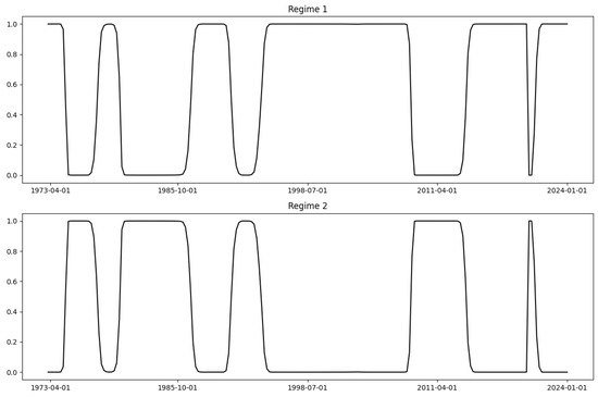
Figure 1.
MS-Regression result of unemployment rate.
In the MS-Regression model for unemployment rate observation value, The log-likelihood of the model is −320.104. The model’s information criteria, including the Akaike Information Criterion (AIC), Bayesian Information Criterion (BIC), and Hannan-Quinn Information Criterion (HQIC), are 650.209, 666.872, and 656.947, respectively. During the modeling process, we found that the results assuming equal variance yielded a higher likelihood compared to those with differing variances. Therefore, the two regimes exhibit the same level of volatility. The parameters are as follows:
Regime 1 Parameters:
Regime 2 Parameters:
Volatility:
Regime Transition Probabilities:
The empirical findings from our model indicate that, during Regime 1, the mean of the unemployment rate model is relatively low, reflecting an economic expansion phase in the U.S. economy. In contrast, during Regime 2, the mean of the unemployment rate model is relatively high, suggesting signs of an economic recession in this phase.
4.2. Result of Quantile-VAR
In our study, we consider the expansion periods (recession periods) across different time frames as continuous time series. Therefore, we integrate the expansion periods (recession periods) from each period into a single time series, resulting in two distinct time series: one for expansion periods and another for recession periods.
Based on the Quantile-VAR model, we set the quantiles at 0.05, 0.5, and 0.95 to model these periods separately. These three models serve to distinguish between the extreme return spillovers associated with negative shocks, average normal conditions, and positive shocks. Consequently, this approach allows us to estimate the correlations under the extreme lower tail, median conditions, and the extreme upper tail. During the estimation process, we select the optimal parameters according to the Schwarz Criterion (SC) for our models. We set the forecast horizon .
Figure A6, Figure A7 and Figure A8 represent the impulse response functions for the entire dataset, expansion periods, and recession periods, respectively. Table 1, Table 2 and Table 3 present the return spillovers in the quantile VAR for the entire dataset, while Table 4, Table 5, Table 6, Table 7, Table 8 and Table 9 provide the return spillovers in the quantile VAR for the expansion periods and recession periods, respectively.

Table 1.
Return spillovers in the quantile VAR (extreme lower quantile = 0.05) for all data.
Table 2.
Return spillovers in the quantile VAR (extreme lower quantile = 0.5) for all data.
Table 3.
Return spillovers in the quantile VAR (extreme lower quantile = 0.95) for all data.
Table 4.
Return spillovers in the quantile VAR (extreme lower quantile = 0.05) for expansion period.
Table 5.
Return spillovers in the quantile VAR (extreme lower quantile = 0.5) for expansion period.
Table 6.
Return spillovers in the quantile VAR (extreme lower quantile = 0.95) for expansion period.
Table 7.
Return spillovers in the quantile VAR (extreme lower quantile = 0.05) for recession period.
Table 8.
Return spillovers in the quantile VAR (extreme lower quantile = 0.5) for recession period.
Table 9.
Return spillovers in the quantile VAR (extreme lower quantile = 0.95) for recession period.
The Impulse Response Function allows for the examination of the individual spillover effects between various currencies at different points in time. However, to observe the impact of each individual currency on all other currencies or to assess the overall effect of all currencies on a single currency, our analysis will focus on the Connectedness Index from Table 1, Table 2, Table 3, Table 4, Table 5, Table 6, Table 7, Table 8 and Table 9. The results indicate that, regardless of whether the full dataset, expansion periods, or recession periods are considered, the TCI is around 70% when the quantile is set at 0.05 or 0.95, and it is approximately 50% when the quantile is set at 0.5. These findings underscore the greater influence of extreme shocks on the system of return spillovers. Notably, the contributions to and from other variables in both the extreme lower and extreme upper tails are significantly stronger compared to those at the median. This result aligns with the findings reported in [1].
Now, we examine the results for the entire dataset. Regardless of the quantile, the impact value of the US dollar on other currencies remains stable around 60. For other currencies, the influence from other currencies is relatively smaller when the quantile is 0.5; however, this influence increases significantly under extreme lower and upper tail conditions. On the other hand, under extreme lower and upper tail conditions, the US dollar’s impact on other currencies is relatively smaller, with the “contribution to others” values being either relatively small or the smallest. In contrast, under median conditions, the US dollar’s impact on other currencies is relatively larger, reaching 80. This suggests that under extreme conditions, there is a stronger mutual influence among various currencies, whereas in normal conditions, the US dollar is the primary factor influencing other currencies. An additional interesting point is that the Australian dollar has a minimal impact on other currencies under normal conditions, with a value of only 21.24.
Next, we observe the results during the expansion period. We find that under extreme lower and upper tail conditions, the US dollar is less influenced by other currencies, whereas under median conditions, the US dollar is most affected by other currencies. Under median and extreme upper tail conditions, the US dollar has the greatest impact on other currencies, but under extreme lower tail conditions, its impact is the smallest. Similarly, it can be observed that under extreme upper and lower tail conditions, the influence of each country’s currency on others expands, while under median conditions, this influence is smaller, with the Australian dollar having the lowest impact at 27.85.
Finally, we examine the results during the recession period. Under median conditions, the US dollar’s influence on other currencies and its susceptibility to influence from other currencies remain the highest. Under extreme lower and upper tail conditions, the mutual influence among various currencies significantly increases, and the degree of influence becomes more similar. The Australian dollar, under median conditions, has the lowest impact on other currencies, with a value of only 2.95.
In the next step, we employed a rolling window analysis to investigate the time-varying characteristics of return spillovers among five currencies. This analysis covers three datasets: the entire dataset, the expansion period, and the recession period, examining the conditions at the median as well as the extreme lower and extreme upper tails. A window size of 20 periods was selected for this analysis. Figure A9 illustrates the changes in TCI for the entire dataset, Figure A10 shows the changes in TCI during the expansion period, and Figure A11 presents the changes in TCI during the recession period.
We found that, compared to the TCI at the median, which exhibits significant fluctuations, the TCI at the extreme lower and extreme upper tails is much higher but with a smaller range of variation. Although the variations at the extreme lower and extreme upper tails are somewhat similar, they do not occur simultaneously when showing larger or smaller values, regardless of whether the entire dataset, the expansion period, or the recession period is considered. Thus, initially, we observed that the TCI at the extreme lower and extreme upper tails shows higher values in any period, but this is not symmetrical. The differences in their behavior can be seen from the TCI graphs, indicating asymmetry between the extreme lower and extreme upper tails.
5. Conclusions
Through the application of MS-Regression, this study successfully identifies the economic crisis cycles using the unemployment rate as the most reliable indicator among the four macroeconomic metrics analyzed. The identified regimes for expansion and recession periods were then utilized to construct time series, which were further analyzed using the Quantile-VAR model. The analysis revealed that, under normal economic conditions, the US dollar plays a dominant role in the system of currency interactions, both in terms of its influence on and its susceptibility to other currencies, with the Australian dollar showing the least impact on others. However, during extreme economic conditions, represented by the extreme lower and extreme upper tails, the mutual influence among different currencies increases, and the relative dominance of the US dollar diminishes. This finding aligns with the conclusions drawn in [10] regarding the spillover effects among EU currencies, indicating that during relatively stable periods of the euro’s existence, the correlation between the new EU forex market and the US dollar is at its peak. In contrast, conditional correlations reach their lowest levels during the Global Financial Crisis and the European debt crisis. Considering that market linkages tend to be stronger during periods of stress than during normal times (as noted by [22]), the observation of stronger linkages in the extreme lower tail is not surprising. However, the changes in TCI between the extreme lower and extreme upper quantiles and the median quantile suggest that the strength of linkages increases with the magnitude of both extreme negative and positive shocks. This is consistent with previous research on contagion effects, which emphasizes the spillover effects of extreme events in both extreme lower and extreme upper quantiles (such as [23]). Moreover, the study found that the spillover effects at the extreme lower and upper tails are asymmetric, as the timing of extreme values does not align (this finding is consistent with the conclusions drawn in [1]), highlighting the complex dynamics of currency interactions under extreme market conditions. These findings contribute to a deeper understanding of how economic crises and extreme market conditions alter the patterns of currency interactions, providing valuable insights for policymakers and investors.
However, our study also acknowledges certain limitations that warrant further consideration. One such issue pertains to the potential significant differences in spillover effects of currency interactions across different quantiles of economic cycles. Our findings reveal asymmetric spillover effects under varying economic conditions, suggesting a need for more in-depth research into this phenomenon.
Moreover, our analysis of spillover effects among various currencies has been conducted using a VAR model based on linear assumptions. However, real-world currency relationships are not strictly linear; thus, it is imperative to explore whether non-linear relationships exist between currencies and to analyze these relationships under both normal and extreme market conditions. Addressing this gap, future research should consider employing Quantile LSTM models (the method is mentioned in [24]). LSTM models have become increasingly popular for studying non-linear relationships through deep learning approaches. By incorporating the loss function of quantile regression into the LSTM framework, we can develop a Quantile LSTM model. This approach would enable the examination of currency interactions at different quantiles, thereby providing a more nuanced understanding of their dynamics.
Author Contributions
Conceptualization, Z.L. and M.T.I.; methodology, Z.L. and M.T.I.; software, Z.L. and M.T.I.; validation, Z.L. and M.T.I.; formal analysis, Z.L. and M.T.I.; investigation, Z.L. and M.T.I.; resources, Z.L. and M.T.I.; data curation, Z.L. and M.T.I.; writing—original draft preparation, Z.L. and M.T.I.; writing—review and editing, Z.L. and M.T.I.; visualization, Z.L. and M.T.I.; supervision, Z.L. and M.T.I.; project administration, Z.L. and M.T.I.; funding acquisition, Z.L. and M.T.I. All authors have read and agreed to the published version of the manuscript.
Funding
This research received no external funding.
Data Availability Statement
Macroeconomic Indicators are available accessed at https://fred.stlouisfed.org/ (accessed on 1 January 2025). All Currencies Data are available at www.investing.com (accessed on 1 January 2025).
Acknowledgments
Thanks to the department of mathematical science, USM for the administrative support of our research.
Conflicts of Interest
The authors declare no conflicts of interest.
Abbreviations
The following abbreviations are used in this manuscript:
| GDP | Gross Domestic Product for United States |
| CPI | Consumer Price Index: All Items: Total for United States |
| dx | the USD Index |
| gbp | British pound |
| aud | Autralian dollar |
| chf | Swiss franc |
| jpy | Japanese yen |
| MS-Regression | Markov Switching Regression |
| Quantile-VAR | Quantile Vector Regression |
| GFEVD | Generalized Forecast Error Variance Decomposition |
| TCI | Total Connectedness Index |
Appendix A. Figures of the Paper

Figure A1.
Level series of each macroeconomic indicator.
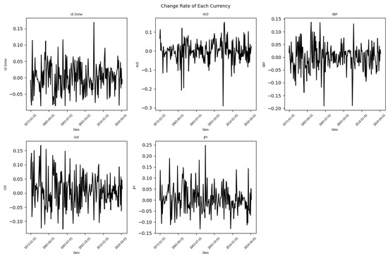
Figure A2.
Change rate of each exchange rate.
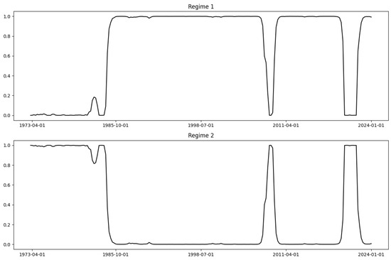
Figure A3.
MS-regression result of GDP.
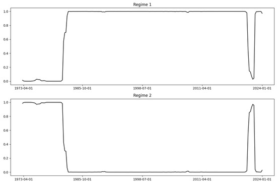
Figure A4.
MS-regression result of CPI.
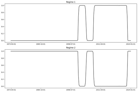
Figure A5.
MS-regression result of Interest Rate.

Figure A6.
Pulse effect of total data.
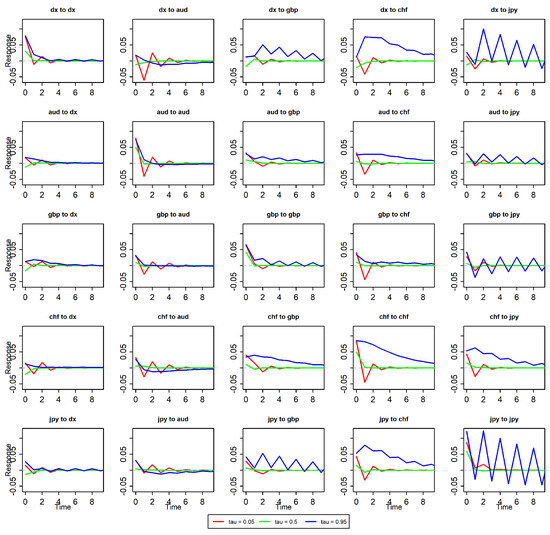
Figure A7.
Pulse effect of expansion period.
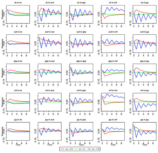
Figure A8.
Pulse effect of recession period.
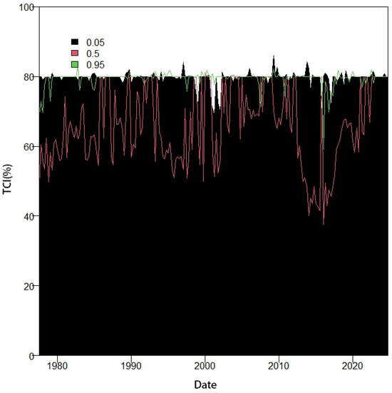
Figure A9.
Window rolling TCI of total data.

Figure A10.
Window rolling TCI of expansion period.

Figure A11.
Window rolling TCI of recession period.
Appendix B. Tables of the Paper
Table A1.
Descriptive statistics for each currency change rate.
Table A1.
Descriptive statistics for each currency change rate.
| dx | aud | gbp | chf | jpy | |
|---|---|---|---|---|---|
| Mean | 0.00066 | −0.00111 | −0.00146 | 0.00875 | 0.00515 |
| Median | −0.00121 | 0.00133 | 0.00077 | 0.00604 | −0.00248 |
| Max | 0.16933 | 0.15196 | 0.13699 | 0.16868 | 0.24821 |
| Min | −0.08654 | −0.29083 | −0.19125 | −0.12751 | −0.13187 |
| Std. Dev. | 0.04386 | 0.05629 | 0.05143 | 0.05733 | 0.06049 |
| Skewness | 0.30783 | −0.91445 | −0.35442 | 0.27245 | 0.65167 |
| Kurtosis | 0.44517 | 3.99390 | 1.26795 | −0.01239 | 1.18898 |
| Jarque-Bera | 5.00 | 167.23 | 18.29 | 2.57 | 26.97 |
| ADF | −13.69 | −15.15 | −13.91 | −13.94 | −5.91 |
Table A2.
Correlation coefficients between currencies change rates.
Table A2.
Correlation coefficients between currencies change rates.
| dx | aud | gbp | chf | jpy | |
| dx | 1.0000 | −0.4685 | −0.7479 | −0.8630 | −0.5823 |
| aud | 1.0000 | 0.3964 | 0.3249 | 0.1787 | |
| gbp | 1.0000 | 0.5705 | 0.3502 | ||
| chf | 1.0000 | 0.5557 | |||
| jpy | 1.0000 |
References
- Bouri, E.; Lucey, B.; Saeed, T.; Vo, X.V. Extreme spillovers across Asian-Pacific currencies: A quantile-based analysis. Int. Rev. Financ. Anal. 2020, 72, 101605. [Google Scholar] [CrossRef]
- Kinkyo, T. Volatility interdependence on foreign exchange markets: The contribution of cross-rates. N. Am. J. Econ. Financ. 2020, 54, 101289. [Google Scholar] [CrossRef]
- Boubaker, H.; Zorgati, M.B.S.; Bannour, N. Interdependence between exchange rates: Evidence from multivariate analysis since the financial crisis to the COVID-19 crisis. Econ. Anal. Policy 2021, 71, 592–608. [Google Scholar] [CrossRef]
- Qureshi, S.; Aftab, M. Exchange rate interdependence in ASEAN markets: A wavelet analysis. Glob. Bus. Rev. 2023, 24, 1180–1204. [Google Scholar] [CrossRef]
- Obstfeld, M.; Zhou, H. The global dollar cycle. Brookings Pap. Econ. Act. 2022, 2022, 361–447. [Google Scholar] [CrossRef]
- Sun, X.; Lu, X.; Yue, G.; Li, J. Cross-correlations between the US monetary policy, US dollar index and crude oil market. Phys. A Stat. Mech. Its Appl. 2017, 467, 326–344. [Google Scholar] [CrossRef]
- Yang, T. How Real Interest Rate Influences Real GDP, CPI and Unemployment Rate in EU countries. Highlights Bus. Econ. Manag. 2024, 24, 1851–1855. [Google Scholar] [CrossRef]
- Kim, C.J.; Piger, J.; Startz, R. Estimation of Markov regime-switching regression models with endogenous switching. J. Econom. 2008, 143, 263–273. [Google Scholar] [CrossRef]
- Chatziantoniou, I.; Gabauer, D.; Stenfors, A. Interest rate swaps and the transmission mechanism of monetary policy: A quantile connectedness approach. Econ. Lett. 2021, 204, 109891. [Google Scholar] [CrossRef]
- Kočenda, E.; Moravcová, M. Exchange rate comovements, hedging and volatility spillovers on new EU forex markets. J. Int. Financ. Mark. Inst. Money 2019, 58, 42–64. [Google Scholar] [CrossRef]
- Kim, B.H.; Kim, H.; Min, H.G. Reassessing the link between the Japanese yen and emerging Asian currencies. J. Int. Money Financ. 2013, 33, 306–326. [Google Scholar] [CrossRef]
- Wang, G.J.; Xie, C. Cross-correlations between Renminbi and four major currencies in the Renminbi currency basket. Phys. A Stat. Mech. Its Appl. 2013, 392, 1418–1428. [Google Scholar] [CrossRef]
- Rahman, A.; Khan, M.A.; Charfeddine, L. Financial development–economic growth nexus in Pakistan: New evidence from the Markov switching model. Cogent Econ. Financ. 2020, 8, 1716446. [Google Scholar] [CrossRef]
- Bojanic, A.N. A Markov-switching model of inflation in Bolivia. Economies 2021, 9, 37. [Google Scholar] [CrossRef]
- Buthelezi, E.M. Impact of government expenditure on economic growth in different states in South Africa. Cogent Econ. Financ. 2023, 11, 2209959. [Google Scholar] [CrossRef]
- McGrane, M. A Markov-Switching Model of the Unemployment Rate. Congressional Budget Office; 2022. Available online: https://www.cbo.gov/publication/57582 (accessed on 8 December 2024).
- Jena, S.K.; Tiwari, A.K.; Abakah, E.J.A.; Hammoudeh, S. The connectedness in the world petroleum futures markets using a Quantile VAR approach. J. Commod. Mark. 2022, 27, 100222. [Google Scholar] [CrossRef]
- Diebold, F.X.; Yilmaz, K. Measuring financial asset return and volatility spillovers, with application to global equity markets. Econ. J. 2009, 119, 158–171. [Google Scholar] [CrossRef]
- Diebold, F.X.; Yilmaz, K. Better to give than to receive: Predictive directional measurement of volatility spillovers. Int. J. Forecast. 2012, 28, 57–66. [Google Scholar] [CrossRef]
- Grobys, K. Are volatility spillovers between currency and equity market driven by economic states? Evidence from the US economy. Econ. Lett. 2015, 127, 72–75. [Google Scholar] [CrossRef]
- Molnár, A.; Vasa, L.; Csiszárik-Kocsír, Á. Detecting business cycles for hungarian leading and coincident indicators with a Markov switching dynamic model to improve sustainability in economic growth. Decis. Mak. Appl. Manag. Eng. 2023, 6, 744–773. [Google Scholar] [CrossRef]
- Ang, A.; Bekaert, G. International asset allocation with regime shifts. Rev. Financ. Stud. 2002, 15, 1137–1187. [Google Scholar] [CrossRef]
- Londono, J.M. Bad bad contagion. J. Bank. Financ. 2019, 108, 105652. [Google Scholar] [CrossRef]
- Zhou, Y.; Liang, S. LSTM Based Quantile Regression Method for Holiday Load Forecasting. In Proceedings of the 2020 IEEE 4th Conference on Energy Internet and Energy System Integration (EI2), Wuhan, China, 30 October–1 November 2020; pp. 2593–2598. [Google Scholar]
Disclaimer/Publisher’s Note: The statements, opinions and data contained in all publications are solely those of the individual author(s) and contributor(s) and not of MDPI and/or the editor(s). MDPI and/or the editor(s) disclaim responsibility for any injury to people or property resulting from any ideas, methods, instructions or products referred to in the content. |
© 2025 by the authors. Licensee MDPI, Basel, Switzerland. This article is an open access article distributed under the terms and conditions of the Creative Commons Attribution (CC BY) license (https://creativecommons.org/licenses/by/4.0/).