The Design of the Flight Corridor for the Terminal Area Energy Management Phase of Gliding Hypersonic Unmanned Aerial Vehicles

Abstract

This paper introduces an innovative approach to optimizing flight corridors under complex constraints, particularly focusing on the Terminal Area Energy Management (TAEM) phases of reusable vehicles, where nominal trajectories may be inadequate due to initial condition and aerodynamic deviations. Leveraging the elegant principles of symmetry, the proposed optimal flight corridor design method, based on the Lagrange multiplier technique, offers a harmonious balance between trajectory accuracy and adaptability. By describing the TAEM flight corridor through a range–altitude profile and utilizing iterative optimization to uphold physical constraints such as dynamic pressure, overload, and roll angle, this method ensures symmetrical alignment of the design parameters. Through a comprehensive analysis of aerodynamic and initial position uncertainties, this method showcases exceptional symmetry in adapting to trajectory design uncertainties. The simulation results demonstrate the resilient nature of the designed flight corridor, capable of seamlessly accommodating initial state deviations and aerodynamic uncertainties. This symmetrical optimization of flight corridors not only enhances trajectory planning and control capabilities during the terminal energy management phase, but also showcases a paradigm shift towards precision and balance in aerospace engineering. Our simulation findings underscore the efficiency of this approach by reducing the flight corridor range by 50% compared to the nominal state while maintaining robustness across deviation conditions, embodying the symmetrical resilience needed for optimal trajectory design.

1. Introduction

Reusable vehicles, as a new type of space transportation system, meet the demands of the aerospace field for fast, economical, and reusable transportation. They hold broad application prospects in fields such as aerospace weapons and high-altitude rapid reconnaissance. The Terminal Area Energy Management (TAEM) phase of gliding reusable vehicles is characterized by a wide flight envelope, large variations in altitude and speed, and drastic changes in flight conditions. At the same time, constraints such as dynamic pressure, overload, and roll angle must be considered to ensure that the vehicle returns to the airfield within the allowable constraints. Therefore, planning a flight corridor that satisfies multiple constraints becomes particularly important.

Research on TAEM phase trajectory design methods has a long history. References [1,2,3,4,5,6,7,8,9,10] divide the TAEM phase into three stages: capture, heading adjustment, and pre-approach. References [11,12,13,14,15] addressed the problem of control failure and aerodynamic deviations by using the OPTG algorithm to modify the pre-determined trajectory, generating a new trajectory online to improve the trajectory’s adaptability to aerodynamic deviations. To enhance trajectory robustness, References [16,17,18,19] studied trajectory generation methods, which improved robustness to flight process deviations. However, these methods impose strict initial state constraints on the TAEM phase. When there are large deviations in the vehicle’s initial position and flight path angle, online trajectory generation technology in the TAEM phase struggles to effectively control robustness, often leading to computational instability because the memory of the flight control computer does not support large computational iterations [20]. To address such problems, Reference [21] proposed the concept of energy corridors by calculating trajectories based on altitude–dynamic pressure profiles to handle deviations in initial conditions and lift-to-drag ratios. Reference [22] introduced a single-parameter iterative trajectory design method to solve the adaptability of trajectories under large deviations in altitude, speed, position, and heading during the initial TAEM phase. Reference [23] proposed a reverse trajectory solution for ground paths during energy management, using Hermite interpolation, to address the issue of nominal trajectories failing to adapt to large initial state and aerodynamic uncertainties. The designed nominal trajectory can adapt to multiple constraints, enabling complex flight missions. References [24,25,26,27] applied numerical optimization algorithms for online trajectory planning. However, these methods showed improved adaptability to initial TAEM deviations caused by re-entry disturbances and various uncertainties, but the real-time performance of online TAEM trajectory planning could not be guaranteed due to the heavy computational load. This limitation significantly reduces the engineering applicability of such methods. Reference [28] addressed the real-time limitations of online trajectory generation methods and their poor practical applicability by adding a linear predictive capture phase before TAEM planning, completing online generation of the TAEM phase trajectory by predicting the end point and state of linear flight, thus alleviating the real-time performance issue. Similarly, Reference [29] established a trajectory database from the perspective of HAC location, constructing the database based on initial altitude, position, heading, and HAC location, using cubic curves to describe the trajectories in the database, ensuring that a suitable trajectory exists even with large initial energy and heading deviations. Reference [30] proposed a fast trajectory generation algorithm using iterative correction, quickly determining the HAC location and final radius to adjust the flight path, ultimately generating a trajectory that meets the constraint requirements. In recent years, TAEM uncertainty and trajectory optimization have seen further advancements. Reference [31] applied reinforcement learning for real-time trajectory adjustments in uncertain environments, enhancing robustness. Reference [32] introduced an adaptive control algorithm to handle aerodynamic uncertainties, improving stability during the TAEM phase.

In summary, current research on TAEM phase trajectory design mainly addresses initial position and state perturbations but often falls short in ensuring robustness under significant deviations. Existing methods typically impose strict initial conditions, limiting their applicability when aerodynamic changes, atmospheric density variations, or large initial deviations are present. Furthermore, these approaches frequently encounter computational instability because of a limitation in the optimization technique, which impacts their effectiveness in real-world scenarios. To bridge these gaps, this paper proposes an optimization analysis method for TAEM flight corridors that ensures robustness under multiple uncertainties. By transforming constraints into a dynamic pressure–altitude profile and using an iterative angle-of-attack approach in combination with the Lagrange multiplier method, we derive an optimal flight corridor that satisfies all constraints. Unlike prior studies, our method fully considers aerodynamic deviations and initial position uncertainties, analyzing their impact comprehensively to ensure the robustness of the designed flight corridor. This approach not only ensures that all constraints are met, but also provides a reliable solution for maintaining trajectory robustness, offering a new perspective on defining the capability boundaries for unpowered flight during the TAEM phase, effectively addressing the shortcomings found in current research.

2. Problem Description of TAEM

In the trajectory design of the vehicle’s TAEM phase, the effects of sideslip angle and the Earth’s curvature are neglected, and the Earth’s rotational angular velocity is considered constant. A kinematic model of the vehicle is established as follows:

$$\left\{\begin{array}{l}\dot{V}={\displaystyle \frac{-D}{m}}-g\sin \gamma \\ \dot{\gamma }={\displaystyle \frac{L\cos \mu }{mV}}+\left({\displaystyle \frac{V}{r}}-{\displaystyle \frac{g}{V}}\right)\cos \gamma \\ \dot{\chi }={\displaystyle \frac{V\cos \gamma \sin \chi \tan \theta }{r}}+{\displaystyle \frac{L\sin \mu }{mV\cos \gamma }}\\ \dot{H}=V\sin \gamma \\ {\dot{P}}_N=V\cos \gamma \cos \chi \\ {\dot{P}}_E=V\cos \gamma \sin \chi \end{array}\right.$$

(1)

where $H$ represents the ellipsoidal altitude, $V$ is the velocity relative to the Earth, $\gamma$ is the flight path angle, $\chi$ is the heading angle, $\theta$ is the pitch angle, $\alpha$ is the angle of attack, $\mu$ is the roll angle, $m$ is the mass, $g$ is the gravitational acceleration at the current altitude, $r$ is the distance from the Earth’s center, $L$ is the lift force, $D$ is the drag force, $P_N$ is the northward distance, and $P_E$ is the eastward distance.

The lift $L$ and drag $D$ are expressed as follows:

$$\left\{\begin{array}{c}L=-F_x\sin \alpha +F_z\cos \alpha \\ D=F_x\cos \alpha +F_z\sin \alpha \end{array}\right.$$

(2)

The axial force $F_x$ and normal force $F_z$ satisfy the following equations:

$$\left\{\begin{array}{l}{F}_x={\displaystyle \frac{1}{2}}\rho V^{2}S{C}_x\\ F_z={\displaystyle \frac{1}{2}}\rho V^{2}S{C}_z\end{array}\right.$$

(3)

where $S$ is the reference area, $\rho$ is the atmospheric density, $C_x$ is the axial aerodynamic force coefficient, and $C_z$ is the normal aerodynamic force coefficient. $C_x$ and $C_z$ all come from wind tunnel experiments of the vehicle, and each of them is a function of the angle of attack and Mach number.

Neglecting the effects of the Earth’s curvature and sideslip can limit the accuracy and applicability of the model, particularly for longer TAEM phases where these factors become more significant.

•1. Impact of Neglecting Earth’s Curvature:

•Limitations: The Earth’s curvature becomes relevant when the flight path covers a large distance. Ignoring this curvature can lead to inaccuracies in altitude, velocity, and distance calculations over longer distances. In the TAEM phase, especially for higher altitudes or extended flight distances, this assumption might cause deviations in trajectory predictions.

•Potential Impact: For longer TAEM phases, the simplified flat Earth assumption could lead to underestimation or overestimation of the vehicle’s position relative to the landing site, reducing landing accuracy. This might affect the ability to meet terminal constraints like velocity and altitude at the designated landing window.

•2. Impact of Neglecting Sideslip:

•Limitations: Sideslip refers to the lateral movement of the vehicle relative to its direction of travel, caused by aerodynamic forces or crosswinds. Ignoring sideslip assumes that the vehicle’s motion is perfectly aligned with its longitudinal axis, which is rarely the case in real-world flight conditions.

•Potential Impact: Neglecting sideslip can underestimate the yawing moments and lateral forces that affect trajectory and control. This could lead to inaccuracies in heading alignment, especially during maneuvers requiring precise control, such as the heading adjustment phase. Over longer TAEM phases, sideslip effects could result in lateral deviations, making it harder to align the vehicle with the runway for a safe landing.

While these simplifications make the model easier to compute, they reduce its accuracy for longer TAEM phases. Ignoring the Earth’s curvature can lead to errors in trajectory prediction over long distances, and neglecting sideslip can affect yaw control, and lateral stability, especially during critical maneuvers. To improve the model’s applicability to longer or more complex TAEM phases, these effects should be considered.

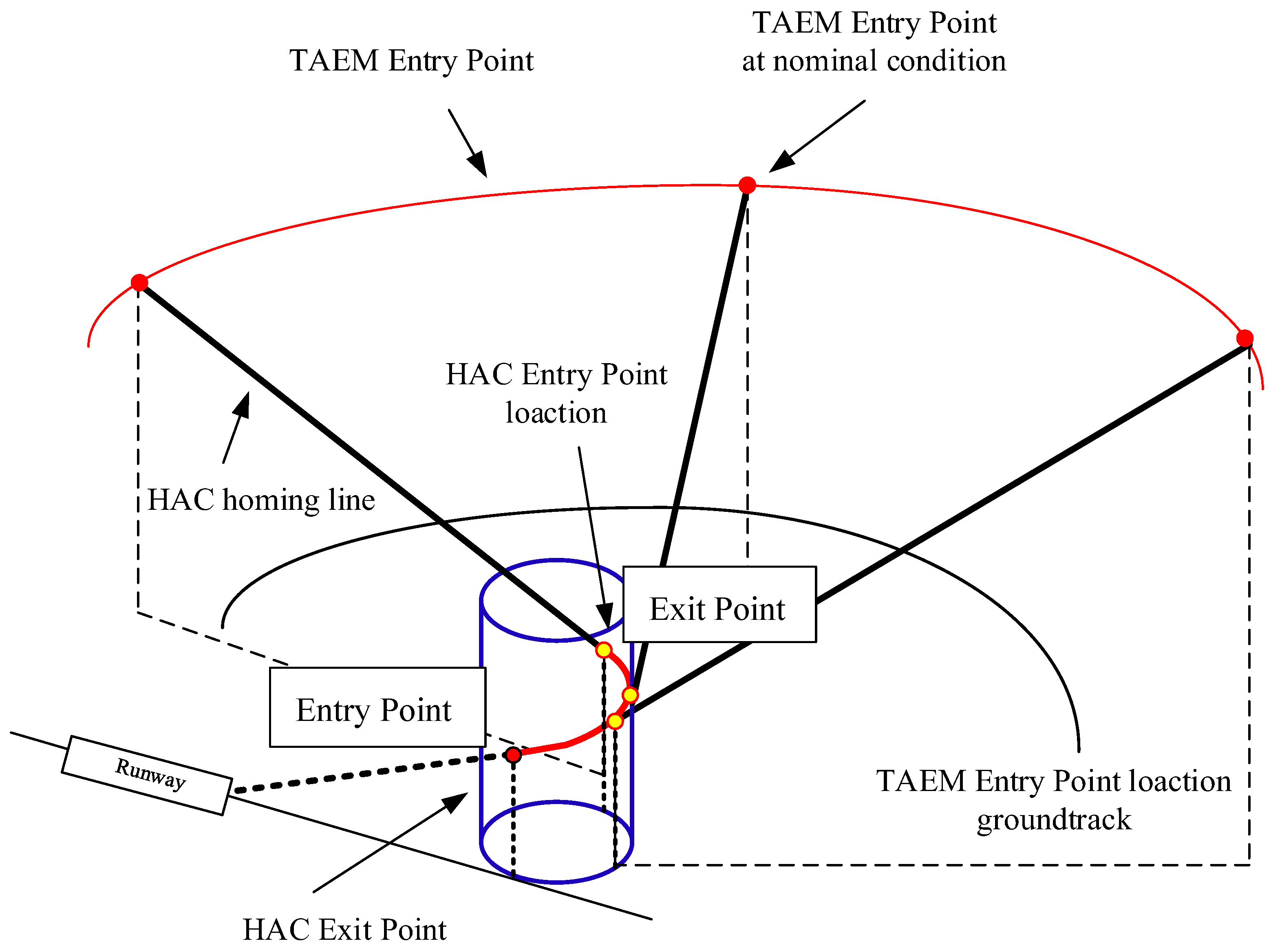
The research on guidance and control methods for the TAEM phase originates from the space shuttle, whose mission profile is shown in Figure 1. The TAEM phase of the space shuttle is divided into four sub-phases: the S-turn phase, heading alignment phase, heading alignment correction phase, and final approach phase. The S-turn phase is used to dissipate excess energy by extending the flight path when the vehicle’s energy is too high; hence, the S-turn is not mandatory. In the heading alignment phase, the vehicle flies toward a pre-designated HAC (heading alignment circle), ensuring that the ground track direction is tangent to the heading alignment circle. After reaching the HAC, the vehicle enters the heading alignment correction phase, during which the vehicle aligns with the runway centerline. The final approach phase further fine-tunes the heading to align with the runway centerline, while ensuring that the vehicle’s altitude, speed, and position meet the requirements for automatic landing.

Throughout the entire TAEM phase, it is crucial to ensure that the vehicle’s overload, dynamic pressure, and roll angle do not exceed the structural strength limits of the vehicle. Furthermore, at the endpoint of the TAEM phase, the vehicle must satisfy the terminal state constraints.

3. Establishment of TAEM Flight Corridor

The TAEM flight corridor can adapt to vehicles with different aerodynamic profiles or mission objectives through the following key adjustments:

•1. Customization of Aerodynamic Models:

•Adaptation: The method relies on aerodynamic coefficients (e.g., lift-to-drag ratio) that can be customized for different vehicles by incorporating vehicle-specific aerodynamic data. These coefficients can be recalculated based on the specific aerodynamic profile of the new vehicle, such as its shape, size, and operational environment (e.g., hypersonic vs. subsonic regimes).

•Process: By updating the aerodynamic coefficients (e.g., lift, drag, and moment coefficients) in the model, the flight corridor can be redefined to accommodate different flight dynamics and performance capabilities.

•2. Adjusting Constraints for Different Missions:

•Adaptation: The method allows flexibility in defining mission-specific constraints, such as dynamic pressure, load factor, and altitude limits, which vary depending on the vehicle’s mission (e.g., space re-entry, reconnaissance).

•Process: For different missions, the boundary conditions of the flight corridor (upper and lower limits) can be redefined to meet the specific operational requirements, such as higher altitudes for space vehicles or tighter maneuverability for atmospheric missions.

•3. Modification of Control Inputs:

•Adaptation: The method can adjust the control strategy based on the vehicle’s control surfaces and propulsion capabilities. For example, a vehicle with limited control surfaces may require different control algorithms compared to a highly maneuverable vehicle.

•Process: Control parameters such as bank angle limits, roll rates, and turn radii can be modified in the iterative calculations to reflect the control characteristics of different vehicles.

•4. Real-Time Adaptability:

•Adaptation: The method can be integrated with real-time control systems, allowing the vehicle to dynamically adjust to changing aerodynamic conditions during flight. This flexibility is crucial for vehicles operating in environments with high uncertainty or varied mission objectives.

•Process: Real-time data feedback and adaptive algorithms (such as machine learning) can adjust the flight corridor and control inputs based on in-flight conditions, making the method adaptable to a wide range of missions and vehicles.

In summary, by updating the aerodynamic coefficients, adjusting the mission constraints, and modifying the control strategies, the method can be tailored to different vehicles and mission objectives, ensuring flexibility across various flight conditions.

3.1. Constraint Analysis

During the TAEM phase of reusable vehicles, multiple constraints must be met, and the vehicle is required to reach the automatic landing window at the end of this phase. To ensure the vehicle safely and accurately arrives at the automatic landing window, dynamic pressure and overload constraints must be imposed. Additionally, throughout the flight, constraints on the angle of attack and roll angle are necessary to maintain the vehicle’s aerodynamic efficiency within controllable limits.

The flight corridor is the set of trajectories that satisfy all of these constraints. Flight corridor planning primarily involves solving for the upper and lower boundaries of the trajectory, ensuring that all trajectories within these boundaries meet the aforementioned constraints. The general mathematical formulation of this problem is as follows:

Differential equation constraints:

$$\dot{x}=f(t,x,u)$$

(4)

Initial state conditions:

$$x\left(t_0\right)=x_0$$

(5)

Process constraints:

$$\mathrm{\Omega }\left(x,u\right)\le 0$$

(6)

Terminal constraints:

$$\mathrm{\Lambda }\left(x\left(t_f\right)\right)\le 0$$

(7)

The specific expression of process constraints is shown in Equation (8):

$$\left\{\begin{array}{l}{\alpha }_{\min }\le \alpha \le {\alpha }_{\max }\\ \overline{q}\le {\overline{q}}_{\max }\\ n_z\le n_{z\max }\\ \mu \le {\mu }_{\max }\end{array}\right.$$

(8)

In this equation, ${\alpha }_{\min }$, ${\alpha }_{\max }$ represent the minimum angle-of-attack constraint and the angle of attack for the maximum lift-to-drag ratio of the control system. ${\overline{q}}_{\max }$ is the maximum dynamic pressure constraint, $n_{z\max }$ is the maximum overload constraint, and ${\mu }_{\max }$ is the maximum roll angle constraint.

$V_{ALIP}$ is the velocity at the entry to the automatic landing phase and serves as a terminal constraint.

3.2. Flight Corridor Description

The flight corridor is the set of trajectories that satisfy constraints on dynamic pressure, overload, angle of attack, roll angle, and terminal conditions. Since all of these constraints are related to altitude and velocity, the flight corridor can be represented in the form of an altitude–velocity profile. Figure 2 shows a schematic diagram of the altitude–velocity corridor. The flight corridor defines the range of velocities at which the vehicle can safely operate at different altitudes. The upper boundary in the diagram represents the maximum flight capability, where the vehicle flies at the angle of attack corresponding to the maximum lift-to-drag ratio. The lower boundary represents the shortest flight distance, where the vehicle flies at the maximum dynamic pressure constraint. If the upper boundary is exceeded, the dynamic pressure acting on the vehicle will surpass its physical limits, potentially leading to structural disintegration. If the lower boundary is exceeded, the vehicle will operate beyond the maximum allowable angle of attack, resulting in a loss of control authority, which may cause control divergence and ultimately lead to the vehicle crashing.

3.3. Flight Corridor Solution Method

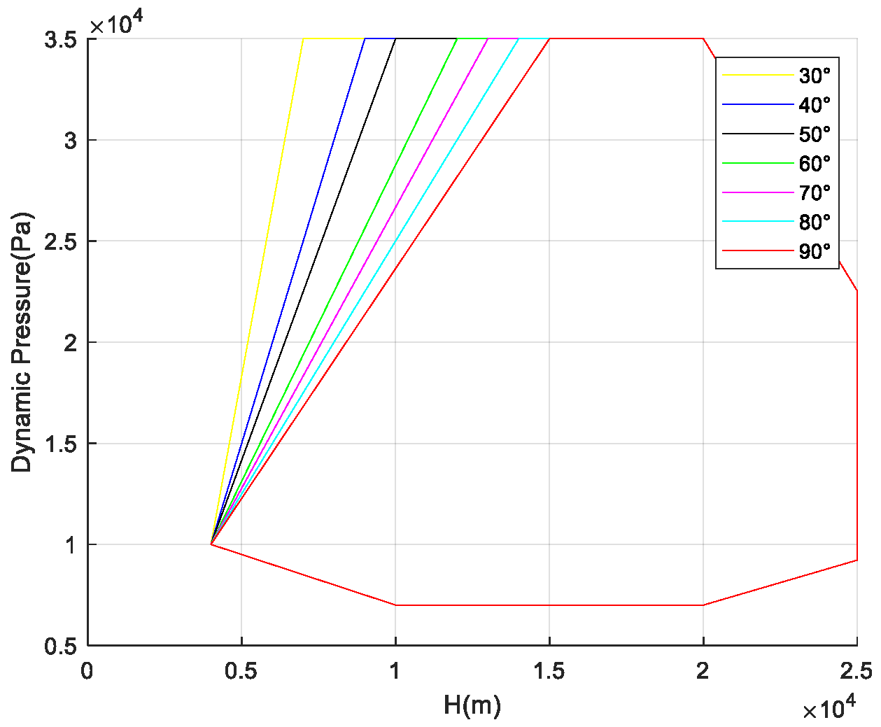
To ensure that the vehicle meets the dynamic pressure constraints during the re-entry process, this section uses dynamic pressure as the design parameter and designs a dynamic pressure guidance profile that satisfies the dynamic pressure limits at different altitude nodes, i.e., a given dynamic pressure–altitude profile.

The dynamic pressure profile is provided in accordance with the method outlined in Reference [23], resulting in the dynamic pressure–altitude profile shown in Figure 3.

The initial altitude and dynamic pressure are denoted as $H_0$ and $q_0$, respectively, while the terminal altitude and dynamic pressure are denoted as $H_f$ and $q_f$, respectively. The dynamic pressure profile can then be described as follows:

$$q=\left\{\begin{array}{cc}{q}_0+{\displaystyle \frac{q_1-q_0}{h_1-h_0}}(h-h_0)& h_1<h<h_0\\ q_1& h_2<h<h_1\\ q_1+{\displaystyle \frac{q_f-q_1}{h_f-h_1}}(h-h_1)& h_f<h<h_2\end{array}\right.$$

(9)

Since dynamic pressure is a function of altitude and velocity, the dynamic pressure–altitude profile can be transformed into a velocity–altitude profile. At each moment, when the velocity and altitude are given, the rate of change in velocity and altitude is known, the angle of attack and flight path angle can be iteratively calculated to fit the given dynamic pressure–altitude profile by calculating the rate of change in velocity and altitude at different time nodes. Simultaneously, a performance index $J$ is introduced, and when $J$ reaches its minimum value of 0, the calculated angle of attack and path angle satisfy the predetermined rates of change for altitude and velocity.

$$J={\left(\dot{H}-{\dot{H}}_c\right)}^2+{\left(\dot{V}-{\dot{V}}_c\right)}^2$$

(10)

The specific calculation process is illustrated in Figure 4.

Therefore, the calculation of the TAEM-phase flight corridor is transformed into an iterative process of varying input parameters, namely $q_1$, $h_1$, and $h_2$, to obtain a profile solution that satisfies the constraints and meets the expected objectives. Due to the challenges of multiple iterative parameters and complex constraints in flight corridor design and the problem that gradient descent is prone to getting stuck in local optima when handling complex multi-dimensional optimization problems, this paper introduces Lagrange multipliers to solve for the upper and lower boundaries of the flight corridor.

Taking the upper boundary as an example, we aim for the vehicle to extend the glide distance as much as possible within a given altitude range with minimal energy consumption. This is achieved by optimizing the vehicle to maintain the best lift-to-drag ratio, thereby maximizing the horizontal flight distance.

Based on the constraint analysis in Section 3.1, we can construct the Lagrange function for calculating the upper boundary:

$$L(x,{\lambda }_i)=J(x)+{\displaystyle \sum _{i=1}^n{\lambda }_i{g}_i(x)}$$

(11)

where $x$ represents the optimization variables, $J(x)$ is the objective function, $g_i(x)$ is the $i$ constraint, and ${\lambda }_i$ is the corresponding Lagrange multiplier for the constraint.

For the calculation of the upper boundary, the optimization variables $x$ are the iterative parameters $q_1$, $h_1$, and $h_2$, with the constraints being the angle of attack for the maximum lift-to-drag ratio ${\alpha }_{\max }$, the maximum load factor $n_{z_{\max }}$, and the maximum bank angle ${\mu }_{\max }$. The initial and final points of the flight range can be used as the initial values for profile iteration.

Then, the Lagrange function can be written as follows:

$$\begin{array}{l}L=W_{TAEM}(H_1,H_2,q_1)+{\lambda }_1{g}_1(\alpha )+{\lambda }_2{g}_2(n_z)+{\lambda }_3{g}_3(\mu )\\ g_1=\begin{array}{cc}\alpha -{\alpha }_{\max }& (g_1\le 0)\end{array}\\ g_2=\begin{array}{cc}{n}_z-n_{z_{\max }}& (g_2\le 0)\end{array}\\ g_3=\begin{array}{cc}\mu -{\mu }_{\max }& (g_3\le 0)\end{array}\end{array}$$

(12)

where $W_{TAEM}$ represents the total range during the TAEM phase.

The iterative parameters and Lagrange multipliers are obtained by taking partial derivatives with respect to $x$:

$$\left\{\begin{array}{c}{\displaystyle \frac{\partial L}{\partial h_1}}={\displaystyle \frac{\partial W}{\partial h_1}}+{\lambda }_1{\displaystyle \frac{\partial g_1}{\partial h_1}}+{\lambda }_2{\displaystyle \frac{\partial g_2}{\partial h_1}}+{\lambda }_3{\displaystyle \frac{\partial g_3}{\partial h_1}}\\ {\displaystyle \frac{\partial L}{\partial h_2}}={\displaystyle \frac{\partial W}{\partial h_2}}+{\lambda }_1{\displaystyle \frac{\partial g_1}{\partial h_2}}+{\lambda }_2{\displaystyle \frac{\partial g_2}{\partial h_2}}+{\lambda }_3{\displaystyle \frac{\partial g_3}{\partial h_2}}\\ {\displaystyle \frac{\partial L}{\partial q_1}}={\displaystyle \frac{\partial W}{\partial q_1}}+{\lambda }_1{\displaystyle \frac{\partial g_1}{\partial q_1}}+{\lambda }_2{\displaystyle \frac{\partial g_2}{\partial q_1}}+{\lambda }_3{\displaystyle \frac{\partial g_3}{\partial q_1}}\end{array}\right.$$

(13)

where ${\displaystyle \frac{\partial L}{\partial h_1}}$, ${\displaystyle \frac{\partial L}{\partial h_2}}$, ${\displaystyle \frac{\partial L}{\partial q_1}}$ represent the gradients of $L$ with respect to each variable.

Let ${\lambda }_i$ be positive numbers. Based on the calculated gradients, $q_1$, $h_1$, and $h_2$ are updated in each iteration as follows:

$$\left\{\begin{array}{l}{h}_{1,k+1}=h_{1,k}+\epsilon \ast {\displaystyle \frac{\partial L}{\partial h_1}}\\ h_{2,k+1}=h_{2,k}+\epsilon \ast {\displaystyle \frac{\partial L}{\partial h_2}}\\ q_{1,k+1}=q_{1,k}+\epsilon \ast {\displaystyle \frac{\partial L}{\partial q_1}}\end{array}\right.$$

(14)

where $\epsilon$ represents the update rate.

The iteration continues using this method until $L$ converges to its maximum value. The detailed calculation process is illustrated in Figure 5.

3.4. Nominal Flight Corridor Design Results

Considering the constraints for the sample vehicle, with a maximum dynamic pressure of 37,000 Pa, a maximum roll angle of 45°, a maximum normal overload of 2.5 g, and initial conditions for automatic landing with an altitude of 4 km and a velocity of 150 m/s, the nominal flight corridor design is carried out based on the aforementioned constraint conditions and the flight corridor solution method. Figure 6, Figure 7, Figure 8, Figure 9, Figure 10, Figure 11, Figure 12 and Figure 13 show the nominal flight corridor design results. 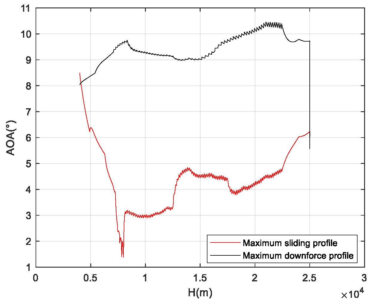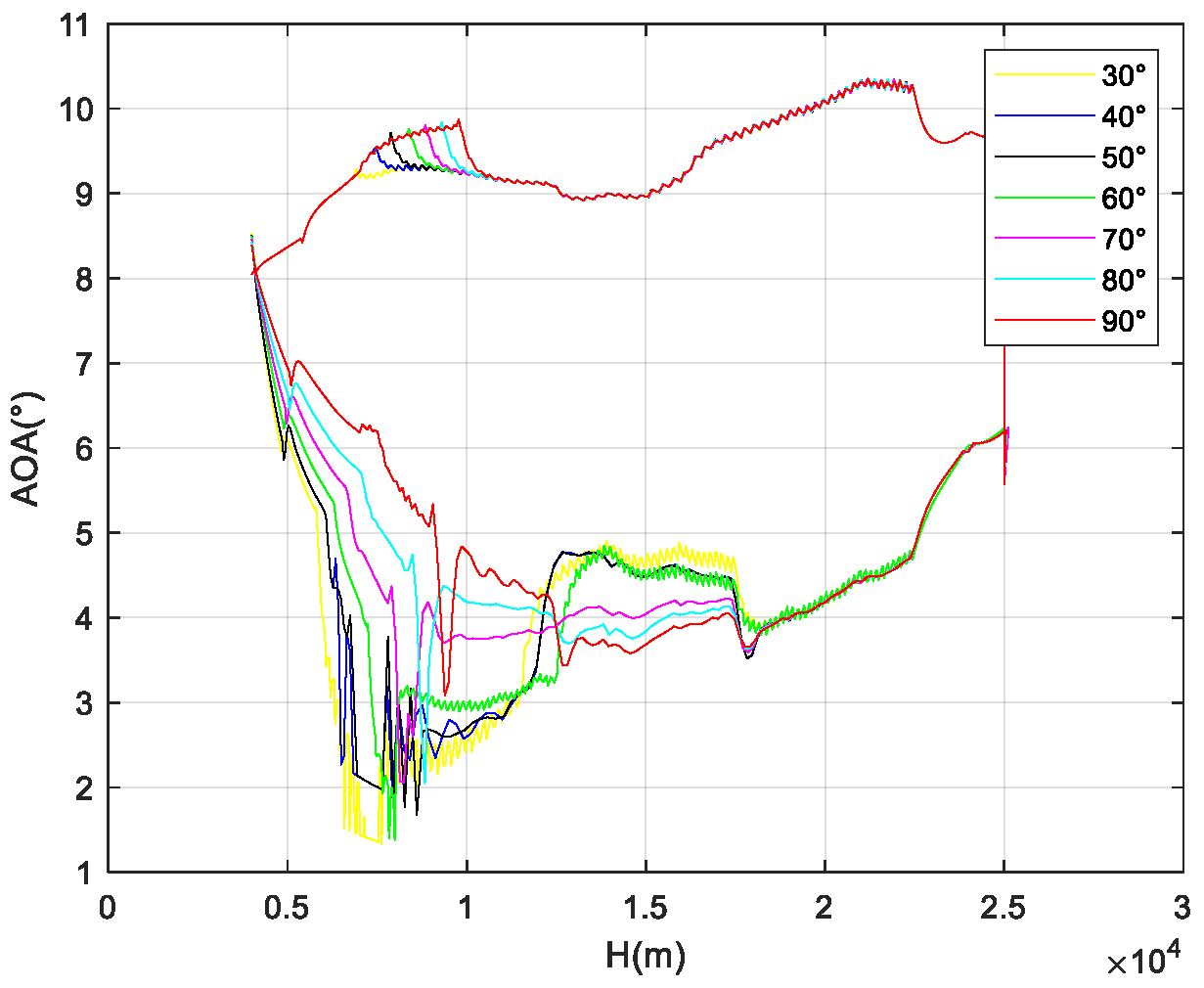Figure 6 presents the angle-of-attack curve of the flight corridor, from which it can be seen that when the vehicle flies along the upper boundary, the flight angle of attack is near the angle of attack corresponding to the maximum lift-to-drag ratio. 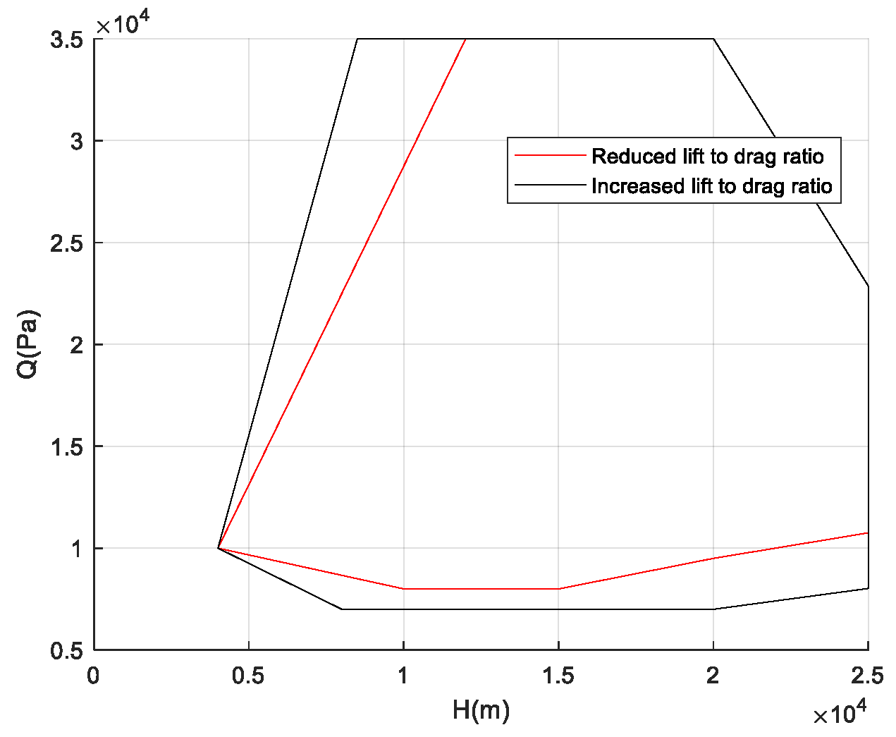Figure 7 presents the dynamic pressure curve of the flight corridor, showing that when the vehicle flies along the lower boundary, the dynamic pressure is close to the maximum dynamic pressure constraint. 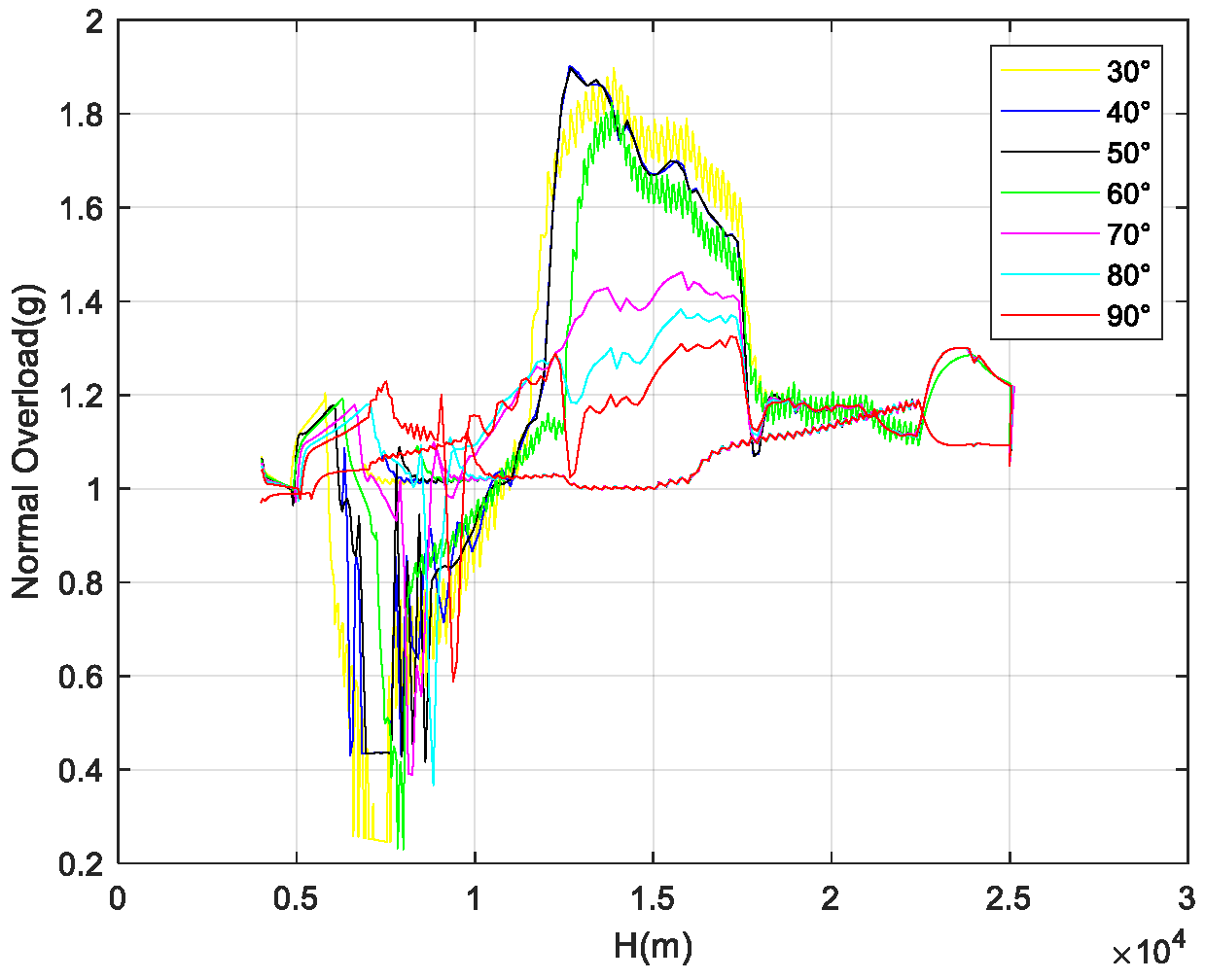Figure 10, Figure 11 and Figure 12 show the fulfillment of the boundary constraints for the flight corridor. According to the results, both the upper and lower boundaries satisfy the process constraints of maximum dynamic pressure, roll angle, and normal overload, with the terminal velocity within the landing window.

4. Flight Corridor Uncertainty Analysis

4.1. Single-Item Uncertainty Analysis

To ensure that the designed trajectory in the TAEM phase has strong robustness, it is necessary to find a flight corridor that satisfies all uncertainty conditions. In this context, robustness refers to the ability of the designed flight corridor to maintain all operational constraints (such as dynamic pressure, overload, and roll angle) in the presence of various uncertainties. These uncertainties include both aerodynamic uncertainties (such as deviations in lift and drag coefficients) and positional uncertainties (such as deviations in the initial altitude and velocity). While the method addresses all forms of uncertainty, particular emphasis is placed on aerodynamic uncertainties, as they tend to have the most significant impact on the flight corridor’s boundaries. Additionally, the flight corridor is designed to prioritize robustness against large deviations in initial conditions, ensuring that even with substantial deviations, the vehicle can still meet all safety and performance constraints during the TAEM phase.

To quantify the robustness of the flight corridor, metrics such as energy consumption, trajectory deviation, and control effort can be used. These metrics provide insight into how well the corridor can handle uncertainties while maintaining vehicle performance and safety. Generally, the wider the flight corridor during the TAEM phase, the stronger its ability to adapt to uncertainties, making it easier to meet the target state constraints and requirements. In actual TAEM-phase flight, certain uncertainties may cause variations in the corridor’s tolerance to uncertainties. These influencing factors can be divided into two main categories: aerodynamic uncertainties and uncertainties in the initial position. Therefore, flight corridor analysis mainly focuses on examining how the corridor changes under different uncertainty conditions and solving for the intersection of flight corridors that satisfies all uncertainties and constraints. Before TAEM, this aircraft is cruising at 25 km high and a 3.5 Ma speed.

(1)

Aerodynamic Uncertainty Analysis

Uncertainties in aerodynamic coefficients, such as lift and drag, can significantly affect vehicle stability and control, especially during the TAEM phase. These uncertainties can lead to the following variations in the predicted aerodynamic forces acting on the vehicle, which, in turn, may cause deviations from the planned trajectory:

• Trajectory Deviation: Uncertainties in lift and drag coefficients can cause unanticipated changes in the vehicle’s flight path. Increased drag, for example, may reduce altitude and range, while variations in lift can affect the vehicle’s ability to maintain the desired flight corridor.
• Control Challenges: Control systems rely on accurate aerodynamic models to adjust control surfaces like elevators and rudders. When aerodynamic coefficients vary unexpectedly, the control system may struggle to compensate, leading to less effective control over pitch, yaw, and roll, potentially causing instability.
• Increased Control Input: To counteract these uncertainties, the control system may need to exert more frequent or stronger inputs, increasing actuator loads and reducing overall control efficiency. This can also lead to more fuel consumption or energy expenditure.
• Potential Instability: Large deviations in aerodynamic coefficients may push the vehicle beyond its stable operating envelope, potentially leading to oscillations or a loss of control. Maintaining stability becomes more difficult as these uncertainties grow, especially during critical maneuvers like heading alignment or final approach.

In summary, aerodynamic uncertainties can compromise both the trajectory accuracy and the vehicle’s ability to maintain stable, controlled flight, requiring more robust control strategies and real-time adjustments.

The consideration of aerodynamic uncertainties in this paper mainly includes deviations in the axial aerodynamic force coefficient, the normal aerodynamic force coefficient, and atmospheric density. When aerodynamic deviations exist, Equation (2) can be rewritten as follows:

$$\left\{\begin{array}{l}L=-(1+k_{C_x})(1+k_{\rho })F_x\sin \alpha +(1+k_{C_z})(1+k_{\rho })F_z\cos \alpha \\ D=(1+k_{C_x})(1+k_{\rho })F_x\cos \alpha +(1+k_{C_z})(1+k_{\rho })F_z\sin \alpha \end{array}\right.$$

(15)

where $k_{C_x},k_{C_z},k_{\rho }$ represent the uncertainties in the axial aerodynamic force coefficient, the normal aerodynamic force coefficient, and atmospheric density, respectively.

Table 1. Deviation range of uncertainty factors.

Uncertainty	Deviation Range
axial aerodynamic force coefficient	−12%~12%
normal aerodynamic force coefficient	−12%~12%
atmospheric density	−10%~10%

provides the range of aerodynamic deviations for a sample vehicle and atmospheric environment. The corresponding flight corridor is designed based on the extreme limits of these uncertainties, and the impact of these uncertainty factors on the flight corridor is analyzed to understand their influence on the flight state.

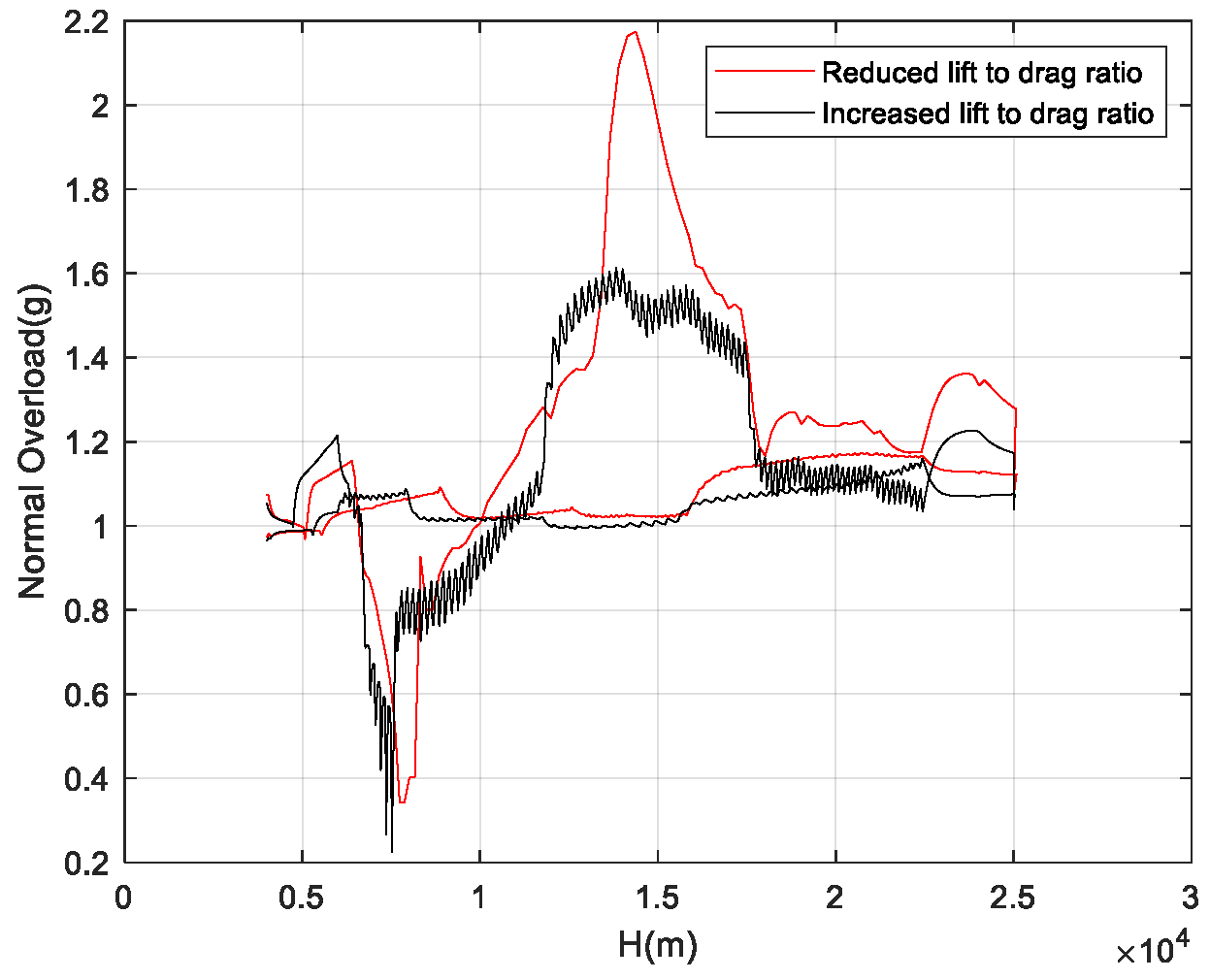
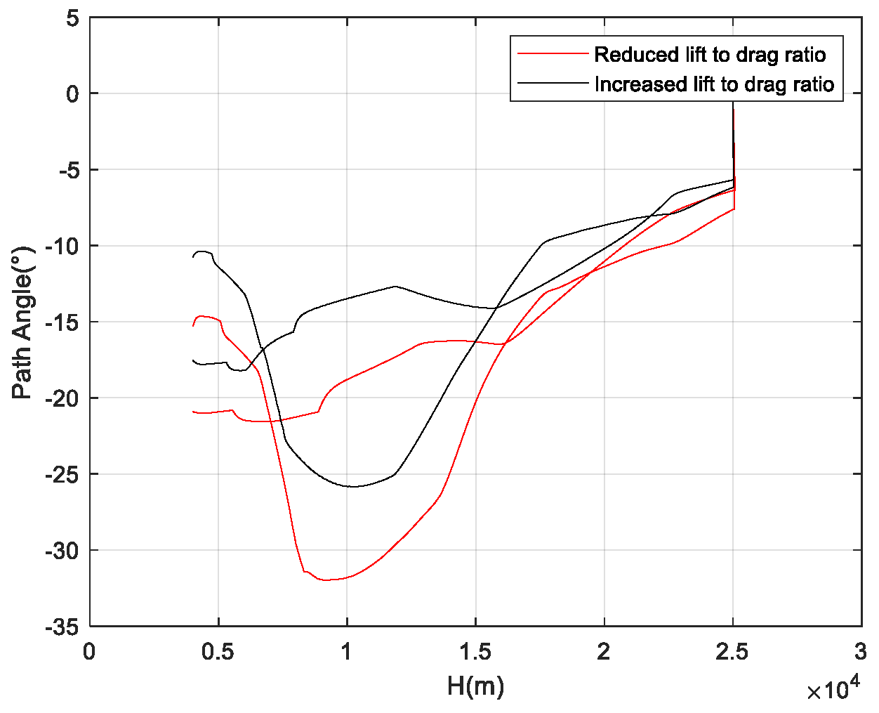
The cases where atmospheric density increases, axial force decreases, and normal force increases (i.e., the lift-to-drag ratio increases), and where atmospheric density increases, axial force increases, and normal force decreases (i.e., the lift-to-drag ratio decreases), represent the most extreme scenarios of aerodynamic uncertainty. 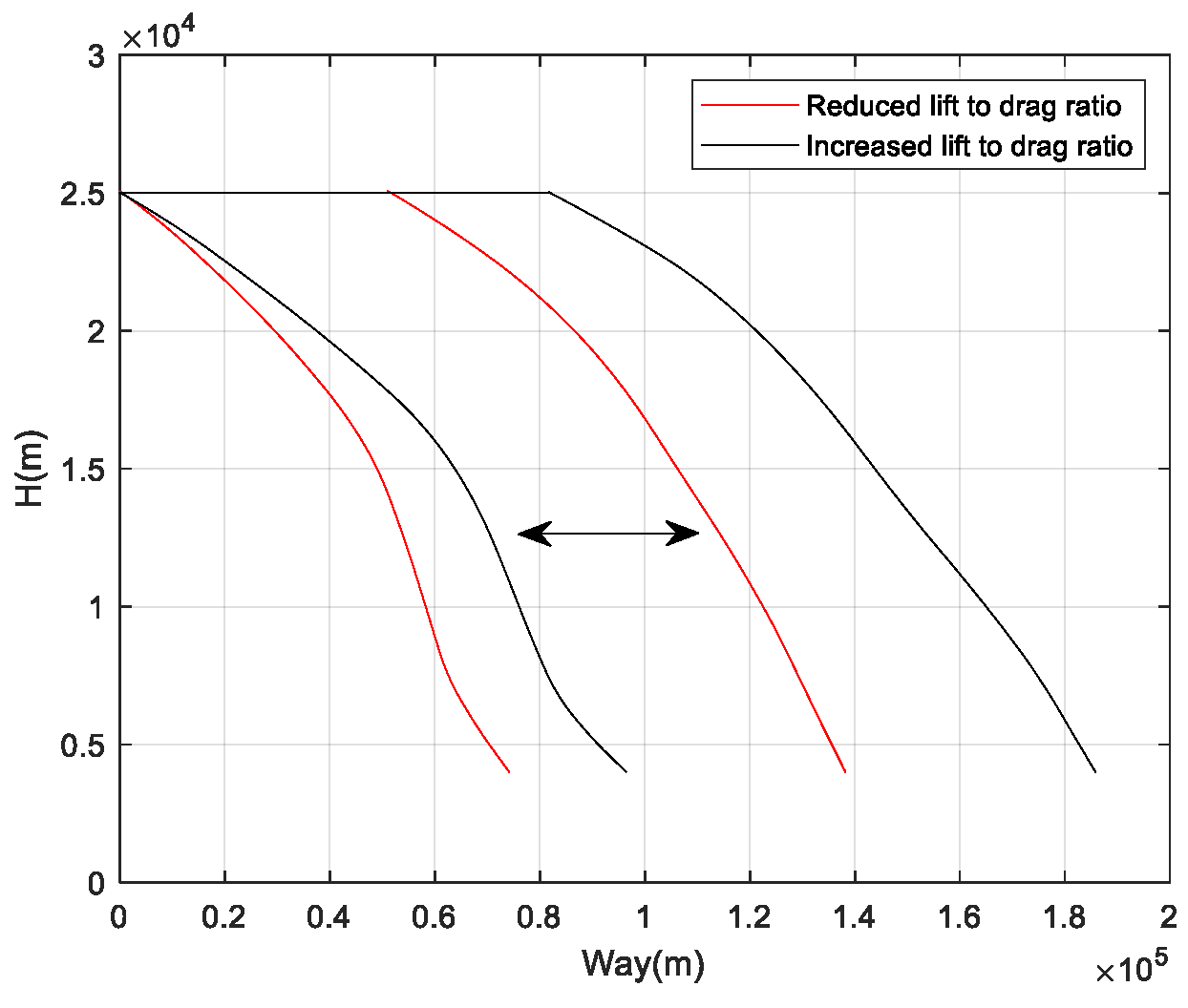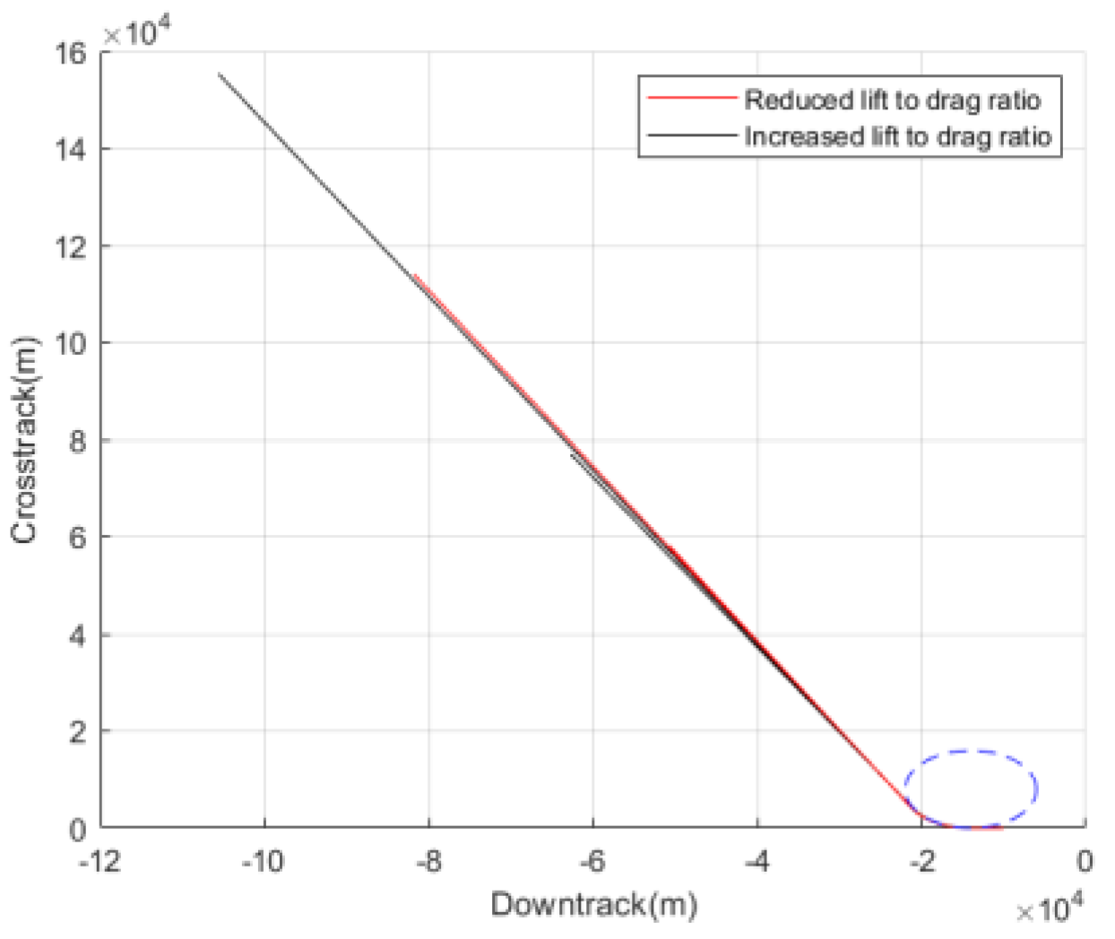Figure 14, Figure 15, Figure 16, Figure 17, Figure 18, Figure 19, Figure 20 and Figure 21 show the flight corridors under these two extreme aerodynamic deviation conditions. As the results indicate, in the case of a decreased lift-to-drag ratio, the flight corridor shifts to the left compared to the nominal case, reducing the vehicle’s flight capability during the TAEM phase. In the case of an increased lift-to-drag ratio, the flight corridor shifts to the right compared to the nominal case, enhancing the vehicle’s flight capability during the TAEM phase.

If the aircraft can have a common corridor solution under different uncertainties, the upper boundary of the flight corridor needs to be taken as the upper boundary when the lift-to-drag ratio decreases, and the lower boundary of the flight corridor needs to be taken as the lower boundary when the lift-to-drag ratio increases. Figure 14 shows the flight corridor that can adapt to the full range of uncertainties. The results reveal that due to the impact of aerodynamic deviations on the flight state, the flight corridor shrinks inward overall, and the range that can cover all uncertainty conditions becomes narrower.

(2)

Initial Position Uncertainty Analysis

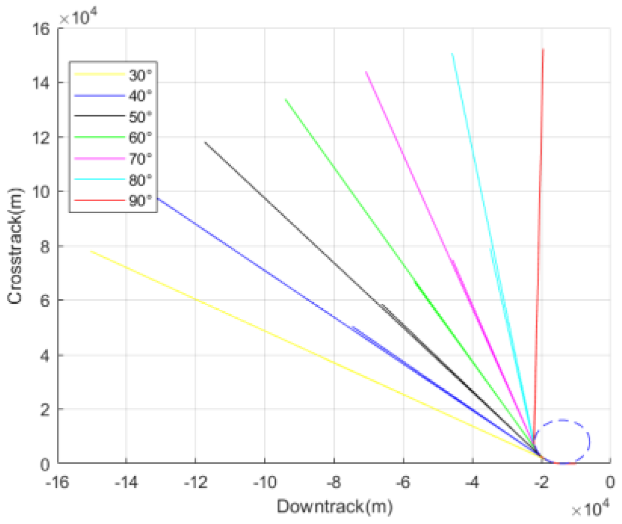
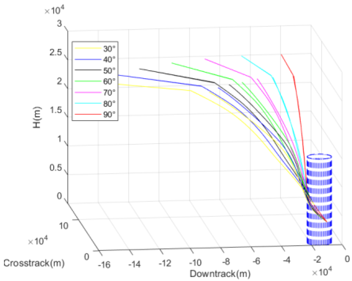
Due to the varying position deviations of the vehicle when entering the TAEM phase, these deviations have different levels of impact on the subsequent heading alignment phase (HAC). Figure 22 shows the influence of different initial TAEM positions on heading alignment when entering HAC. Different initial positions correspond to different required bank angles during the heading alignment phase. The larger the required bank angle, the higher the altitude and velocity when entering HAC. Consequently, the larger the bank angle needed for heading alignment, the more restricted it is by the physical structure of the sample vehicle. The maximum allowable bank angle during the entire TAEM phase for the vehicle is 45°.

Considering that the entry point of the TAEM phase is distributed along a circular arc with a 60° angle, the flight corridor that can accommodate all deviation conditions is analyzed based on different initial positions. Figure 23, Figure 24, Figure 25, Figure 26, Figure 27, Figure 28, Figure 29 and Figure 30 show the results of the flight corridor under initial position deviations. According to the simulation results, when the required bank angle is larger than the nominal state, the lower boundary of the flight corridor shrinks upward, but there is minimal impact on the upper boundary. When the required bank angle is smaller than the nominal state, the lower boundary of the flight corridor expands downward, with no effect on the upper boundary.

Figure 24 and Figure 29 show the dynamic pressure profiles and bank angle curves during flight for different positions. The simulation results meet the constraints of maximum bank angle and dynamic pressure. It can be observed that in order to meet the bank angle constraint, the dynamic pressure during the heading alignment phase is smaller when the required bank angle is large compared to when the required bank angle is small. The simulation results are consistent with the analysis.

4.2. Combination Uncertainty Analysis

Since the deviations encountered by the vehicle during the TAEM phase are the result of multiple combined factors, the flight corridor must be able to adapt to all uncertainty conditions while satisfying the constraints. Based on the above analysis, there are eight extreme cases under combined uncertainties, namely an increased (or decreased) lift-to-drag ratio, and an increased (or decreased) bank angle caused by position deviations. The eight extreme cases were selected based on a combination of the most critical uncertainties affecting the TAEM phase, specifically aerodynamic and positional deviations. These cases represent the worst-case scenarios where aerodynamic coefficients (such as the lift-to-drag ratio) and initial position deviations (altitude, velocity, and heading angle) are at their maximum and minimum bounds. This selection ensures that the flight corridor can accommodate the full range of potential deviations. The methodology for selecting these cases follows standard procedures for extreme case analysis, where the upper and lower bounds of key parameters are tested to ensure robustness across the entire flight envelope.

The goal of flight corridor design is to find the intersection of corridors that satisfies all uncertainty conditions. By calculating the intersection of the flight corridors that can accommodate the maximum aerodynamic and initial position deviations, it is ensured that the vehicle can fly within a safe corridor under any deviation in actual flight. Therefore, calculations are performed based on the aforementioned eight extreme cases and the nominal case. Figure 31 shows the TAEM flight corridors under different extreme conditions, this corridor can meet all uncertainty conditions and constraints, and the designed trajectory within this corridor exhibits the highest robustness. Figure 32, Figure 33, Figure 34, Figure 35, Figure 36, Figure 37 and Figure 38 provide the bank angle, dynamic pressure, and angle-of-attack curves for the upper and lower boundaries of the corridor, with the simulation results of both boundaries meeting the constraint requirements.

5. Conclusions

This paper investigates the altitude–dynamic pressure flight corridor planning for the Terminal Area Energy Management (TAEM) phase of reusable vehicles and its adaptability to uncertainties. By analyzing multiple constraints, including dynamic pressure, load factor, and angle of attack, a flight corridor generation method based on angle-of-attack iteration is proposed. The combined effects of aerodynamic and initial position uncertainties are evaluated, and a flight corridor intersection that accommodates all uncertainty conditions is constructed, ensuring safety and robustness during flight. While the proposed method shows promising results, future work could focus on real-time testing to further validate its performance under dynamic conditions. The use of adaptive control algorithms allows the vehicle to respond to deviations dynamically. These algorithms, such as model predictive control (MPC) or reinforcement learning-based control, can predict future states and make real-time adjustments to the control surfaces or propulsion system to maintain the trajectory within the flight corridor. Additionally, integrating machine learning techniques may improve the prediction of uncertainties and allow for adaptive control, enhancing both robustness and operational efficiency.