Model Error Modeling for a Class of Multivariable Systems Utilizing Stochastic Embedding Approach with Gaussian Mixture Models

Abstract

Many real-world multivariable systems need to be modeled to capture the interconnected behavior of their physical variables and to understand how uncertainty in actuators and sensors affects the system dynamics. In system identification, some estimation algorithms are formulated as multivariate data problems by assuming symmetric noise distributions, yielding deterministic system models. Nevertheless, modern multivariable systems must incorporate the uncertainty behavior as a part of the system model structure, taking advantage of asymmetric distributions to model the uncertainty. This paper addresses the uncertainty modeling and identification of a class of multivariable linear dynamic systems, adopting a Stochastic Embedding approach. We consider a nominal system model and a Gaussian mixture distributed error-model driven by an exogenous input signal. The error-model parameters are treated as latent variables and a Maximum Likelihood algorithm that functions by marginalizing the latent variables is obtained. An Expectation-Maximization algorithm that jointly uses the measurements from multiple independent experiments is developed, yielding closed-form expressions for the Gaussian mixture estimators and the noise variance. Numerical simulations demonstrate that our approach yields accurate estimates of both the multivariable nominal system model parameters and the noise variance, even when the error-model non-Gaussian distribution does not correspond to a Gaussian mixture model.

1. Introduction

The field of system identification focuses on the development and analysis of estimation methodologies for system models using experimental data, i.e., estimating the set of system models that best fit measurements [1,2,3,4]. The formulation of system identification algorithms is generally based on a stochastic problem, where measurement errors are treated as stochastic processes that can affect the accuracy of the estimates of the system model parameters. The measurement error behavior, modeled as Gaussian or other symmetric distributions [1,5], is a classical assumption for the development of estimation algorithms. However, real-world dynamic systems can be affected by uncertainty sources with asymmetric distribution behavior, and the estimation algorithms perform poorly under symmetric distribution assumptions [6]. In this context, it is crucial to address the asymmetries in error models, especially for multiple-input multiple-output (MIMO) systems that require more flexible representation of the uncertainty behavior.

Many system identification algorithms in the literature have been developed under the Maximum Likelihood (ML) principle, motivated by its valuable statistical properties [1,3]. This approach has been used in various fields of application under symmetric and asymmetric distribution assumptions, ranging from modeling simple single-input single-output (SISO) systems, such as dynamic systems with a Finite Impulse Response (FIR) structure [7], systems with quantized data [8], non-linear systems [9,10], astronomy [11,12], estimation [13], medicine [14], and communications [15], among others. Similarly, ML estimation approaches in the time domain [1,2] and the frequency domain [16] have been considered for MIMO systems, with applications in robust control [17,18], power electronics [19,20], and biomedical engineering [21], to mention a few.

In particular, ML estimators are asymptotically unbiased—that is, the estimated values approach the true values when the number of measurements is large. Nevertheless, if the set of measurements is small, the estimates deviate from the true values as a result of the measurement noise variance [1,2]. However, there are scenarios in which a large number of measurements are available and the estimated models change between estimations because there exist sources of uncertainty that the system model does not incorporate [22,23]. In [24], the authors proved that Bayesian methods yield more accurate estimates than classical ML estimation when a kind of exponential distribution assumption is considered to handle censoring data. In [25], the analysis of various approaches to estimate the parameters of a class of exponential distribution was addressed. The authors considered censored samples with mechanical and medical data, obtaining better performance using a Bayesian approach with asymmetry assumptions than using the ML method.

To illustrate the behavior of biased ML estimates, we consider the discrete-time system models shown in Figure 1 as two-input and two-output ($2\times 2$) MIMO linear dynamic systems, where $y_t\in {\mathbb{R}}^2$ is the output signal, $u_t\in {\mathbb{R}}^2$ denotes the input deterministic signal, ${\omega }_t\in {\mathbb{R}}^2$ is the measurement noise signal, and $q^{-1}$ corresponds to the backward shift operator ($q^{-1}{x}_t=x_{t-1}$). The main goal is to obtain an ML estimate of the vector of parameters, $\theta$, that parameterizes the MIMO system model $G_0(q^{-1},\theta )$. The estimates are computed from the measurement set $\{y_{1:N},u_{1:N}\}$ for both the system model shown in Figure 1a, referred to as Model I, and in Figure 1b, called Model II, where N is the data length. Without loss of generality, we assume that all transfer functions in Figure 1 are second-order FIR–MIMO systems. For Model I, an additive measurement noise ${\omega }_t$ is considered. Similarly, for Model II, we add the term $G_{\Delta }(q^{-1},\theta )$, parameterized by a stochastic vector of parameters $\eta$, which models structural and parametric uncertainties in the MIMO system.

We perform 50 numerical simulations to obtain different data sets $\{y_{1:N},u_{1:N}\}$. Then, for each data set, the MIMO system model, $G_0(q^{-1},\theta )$, is estimated for both Model I and Model II using the Prediction Error Method (PEM) for MIMO systems [2]. The principal gains for each estimated MIMO system model are computed. 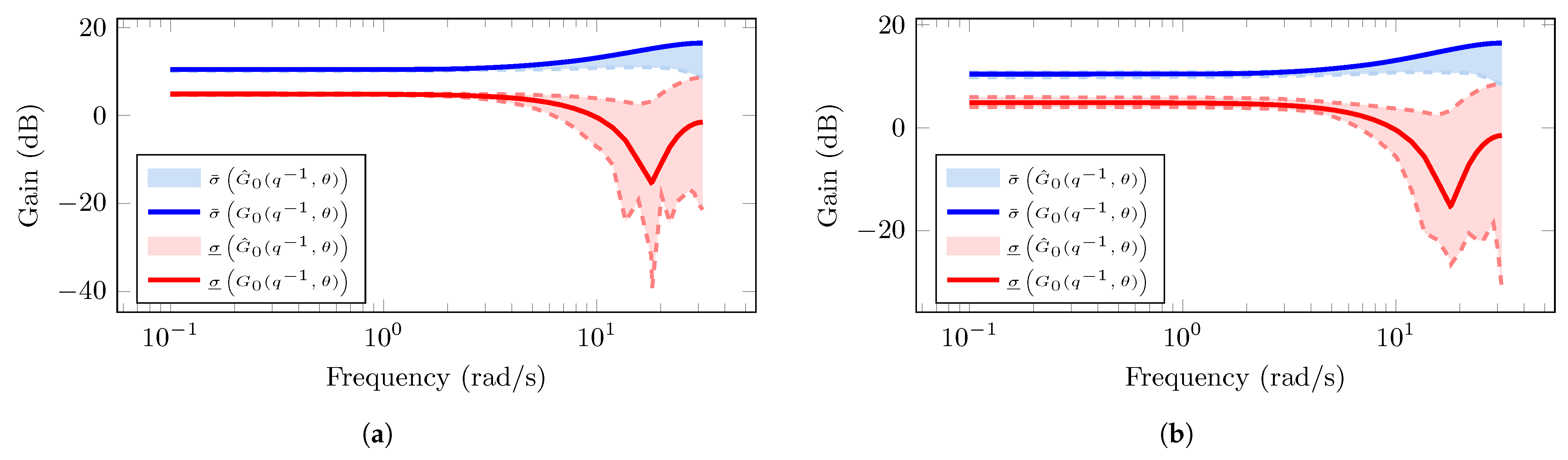The principal gains are important characteristics used to assess the robustness of the system model to plant variations, its sensitivity to disturbances, and for designing robust multivariable control strategies to ensure stability and performance margins [19,26,27]. In Figure 2 and Figure 3, the blue and red shaded regions represent the area in which the magnitudes of the largest, $\overline{\sigma }\left({\widehat{G}}_0(q^{-1},\theta )\right)$, and smallest, $\underline{\sigma }\left({\widehat{G}}_0(q^{-1},\theta )\right)$, principal gains, respectively, of 50 estimations lie. The solid lines (blue and red colors) represent the principal gains of the true MIMO system model $G_0(q^{-1},\theta )$. In Figure 2a, we observe small estimation biases when the number of measurements used for the ML estimations is large ($N={10}^3$). These biases increase as the number of measurements decreases ($N=50$), as shown in Figure 2b. In contrast, in Figure 3, given the incorporation of parametric uncertainties with the term $G_{\Delta }(q^{-1},\theta )$, the estimated MIMO system model yields biased principal gains for both large and small data lengths (see Figure 3a and Figure 3b, respectively). Based on this, it is desirable to develop system identification methodologies to provide estimated models capable of quantifying the error-model that provides parametric and/or structural uncertainties.

One alternative is to consider the uncertainty model as part of the estimation algorithm, combining a nominal model with an error-model. This idea can be adopted for designing robust control systems based on the ${\mathcal{H}}_{\infty }$ norm [28,29] or variable–structure controllers [30]. This approach to model error modeling has been addressed using a deterministic framework, in which the error model is bounded by a set of possible solutions [31]. However, this methodology has been developed for SISO system models and also does not guarantee that the set of solutions adequately describes the uncertainty in the corresponding dynamic system. In [23], the uncertainty modeling is based on residual dynamics calculated from an available nominal SISO system model using PEM.

On the other hand, the Stochastic Embedding (SE) approach has been used to describe uncertainty in dynamic systems by assuming that the system model is a realization that belongs to a probability space and that the parameters that define the error-model are characterized by a probability density function (PDF). In this context, the error-model can be quantified utilizing an ML estimation that treats the error-model parameters as hidden (latent) variables and then solving the associated optimization problem via the Expectation-Maximization (EM) [32] algorithm under Gaussian assumptions for the error-model distribution [33]. In [34], a Bayesian approach is adopted to jointly characterize the nominal system model and the error-model as realizations of random variables under certain prior distributions; then, the posterior distributions of the system model parameters are estimated. However, this approach does not provide a separate derivation of a nominal system model and an error-model.

In [35], a more flexible scenario is proposed in which the error-model distribution can be represented as a Gaussian Mixture Model (GMM). Then, an iterative EM-based algorithm is developed to solve the estimation problem for both the parameters of the nominal system model and the Gaussian mixture parameters that define the error-model distribution. GMMs have traditionally been used in filtering [36,37], communications [38], tracking [39], and probabilistic modeling [40], among others. The flexibility of GMMs lies in the fact that they can approximate non-Gaussian PDFs according to the Wiener approximation theorem, which establishes that any PDF with compact support can be approximated as a linear combination of Gaussian distributions [41]. This idea has been utilized to develop estimation algorithms under non-Gaussian assumptions for dynamic systems (see, e.g., [6]). However, this approach has been considered only for a SISO dynamic system with a multiplicative error-model structure.

In this paper, we extend the SE approach adopted in [35] to a class of MIMO linear dynamic systems considering an additive or a multiplicative structure for modeling the error-model term under non-Gaussian assumptions. We develop an ML estimation algorithm with the SE framework to estimate separately the MIMO nominal system model and the non-Gaussian multivariate error-model distribution as a GMM. Combining the SE approach with a linear combination of Gaussian distributions produces flexible scenarios in which the non-Gaussian distribution that describes the uncertainty is not a GMM but can be approximated by one. The main contributions of the paper are the following:

(a)

A Maximum Likelihood methodology using the SE approach is developed to model parametric and structural uncertainties in a class of MIMO linear dynamic systems. The resulting estimated model combines a nominal MIMO model with an additive or multiplicative multivariate error-model distribution represented as a GMM.

(b)

An iterative EM-based algorithm is proposed to solve the optimization problem associated with the ML estimation, obtaining the estimator for the MIMO nominal system model parameters and closed-form expressions for the estimators of the multivariate GMM parameters that characterize the error-model PDF.

The paper is organized as follows: Section 2 outlines the problem of interest, which considers modeling the error-model for MIMO linear dynamic systems using the SE approach. In Section 3, the estimation problem using the ML principle within GMMs is addressed. In Section 4, an iterative EM-based algorithm is developed to address the associated ML estimation problem. Numerical simulations, considering scenarios with additive and multiplicative uncertainty models, are shown in Section 5. Finally, in Section 6, we present our conclusions.

2. Stochastic Embedding Approach for Class of Multivariable Systems

2.1. System of Interest

The MIMO dynamic system of interest is given by

$$y_t^{\left[r\right]}=G^{\left[r\right]}\left(q^{-1}\right)u_t^{\left[r\right]}+{\omega }_t^{\left[r\right]},$$

(1)

where $q^{-1}$ is the backward operator ($x_t{q}^{-1}=x_{t-1}$), $y_t^{\left[r\right]}\in {\mathbb{R}}^{\tilde{N}\times 1}$ represents the output signal, $u_t^{\left[r\right]}\in {\mathbb{R}}^{\tilde{N}\times 1}$ is the input signal, ${\omega }_t^{\left[r\right]}\in {\mathbb{R}}^{\tilde{N}\times 1}$ is a zero-mean Gaussian white noise with covariance matrix ${\sigma }^2{I}_{\tilde{N}}$ (i.e., $\mathcal{N}({\omega }_t;0,{\sigma }^2{I}_{\tilde{N}})$), and $\tilde{N}$ is the number of inputs and outputs in the multivariable dynamic system. The matrix $G^{\left[r\right]}\left(q^{-1}\right)\in {\mathbb{R}}^{\tilde{N}\times \tilde{N}}$ is the multivariable dynamic model, where each component, $G_{ij}^{\left[r\right]}\left(q^{-1}\right)$, corresponds to the dynamic model relating the i-th output signal to the j-th input signal. The ${\mathrm{superscript} }^{\left[r\right]}$ corresponds to the r-th experiment carried out to obtain the data set $\{u_{1:N}^{\left[r\right]},y_{1:N}^{\left[r\right]}\}$ with $r=1,\dots ,M$. In this case, $u_{1:N}^{\left[r\right]}$ and $y_{1:N}^{\left[r\right]}$ correspond to the measurements $u_t^{\left[r\right]}$ and $y_t^{\left[r\right]}$ with $t=1,\dots ,N$ for each experiment r.

On the other hand, the MIMO system $G^{\left[r\right]}\left(q^{-1}\right)$ in (1) can be represented utilizing a nominal model with an additive error-model as follows [26,42]:

$$G^{\left[r\right]}\left(q^{-1}\right)=G_0(q^{-1},\theta )+G_{\Delta }(q^{-1},{\eta }^{\left[r\right]}),$$

(2)

or a multiplicative error-model given by

$$G^{\left[r\right]}\left(q^{-1}\right)=G_0(q^{-1},\theta )\left[I+G_{\Delta }(q^{-1},{\eta }^{\left[r\right]})\right]\vee \left[I+G_{\Delta }(q^{-1},{\eta }^{\left[r\right]})\right]G_0(q^{-1},\theta ),$$

(3)

where $G_0(q^{-1},\theta )\in {\mathbb{R}}^{\tilde{N}\times \tilde{N}}$ is the nominal model parameterized by $\theta$, and $G_{\Delta }(q^{-1},{\eta }^{\left[r\right]})\in {\mathbb{R}}^{\tilde{N}\times \tilde{N}}$ represents an additive error-model (2) or a multiplicative error-model (3) parameterized by ${\eta }^{\left[r\right]}$. Here, I denotes the identity matrix of appropriate dimensions. The additive error-model in (2) is typically utilized in robust stabilization formulations [43]. The multiplicative uncertainties in (3) provide a more realistic scenario, since they account for the possibility that the error-model in the system may occur at both the input and output of the MIMO system model [43,44]. The nominal model, $G_0(q^{-1},\theta )$, in (2) and (3) is given by the following:

$$G_0(q^{-1},\theta )=\left[\begin{array}{cccc}{G}_{0,11}(q^{-1},{\theta }_{11})& G_{0,12}(q^{-1},{\theta }_{12})& \cdots & G_{0,1\tilde{N}}(q^{-1},{\theta }_{1\tilde{N}})\\ G_{0,21}(q^{-1},{\theta }_{21})& G_{0,22}(q^{-1},{\theta }_{22})& \cdots & G_{0,2\tilde{N}}(q^{-1},{\theta }_{2\tilde{N}})\\ ⋮& \cdots & \cdots & ⋮\\ G_{0,\tilde{N}1}(q^{-1},{\theta }_{\tilde{N}1})& G_{0,\tilde{N}2}(q^{-1},{\theta }_{\tilde{N}2})& \cdots & G_{0,\tilde{N}\tilde{N}}(q^{-1},{\theta }_{\tilde{N}\tilde{N}})\end{array}\right],$$

(4)

with

$$G_{0,ij}(q^{-1},{\theta }_{ij})={\displaystyle \frac{B_{ij}(q^{-1},{\theta }_{ij})}{A_{ij}(q^{-1},{\theta }_{ij})}},$$

(5)

$$B_{ij}(q^{-1},{\theta }_{ij})=b_{1,ij}{q}^{-1}+b_{2,ij}{q}^{-2}+\cdots +b_{n_b,ij}{q}^{-n_{b,ij}},$$

(6)

$$A_{ij}(q^{-1},{\theta }_{ij})=1+a_{1,ij}{q}^{-1}+a_{2,ij}{q}^{-2}+\cdots +a_{n_a,ij}{q}^{-n_{a,ij}},$$

(7)

$${\theta }_{ij}={\left[b_{1,ij}{b}_{2,ij}\cdots b_{n_b,ij}{a}_{1,ij}{a}_{2,ij}\cdots a_{n_a,ij}\right]}^T,$$

(8)

where ${\theta }_{ij}\in {\mathbb{R}}^{(n_{a,ij}+n_{b,ij})\times 1}$, $i=1,2,\cdots ,\tilde{N}$, and $j=1,2,\cdots ,\tilde{N}$. The  error-model $G_{\Delta }(q^{-1},{\eta }^{\left[r\right]})$ in (2) and (3) is assumed to be a linear regression model given by

$$G_{\Delta }(q^{-1},{\eta }^{\left[r\right]})=\left[\begin{array}{cccc}{G}_{\Delta ,11}(q^{-1},{\eta }_{11}^{\left[r\right]})& G_{\Delta ,12}(q^{-1},{\eta }_{12}^{\left[r\right]})& \cdots & G_{\Delta ,1\tilde{N}}(q^{-1},{\eta }_{1\tilde{N}}^{\left[r\right]})\\ G_{\Delta ,21}(q^{-1},{\eta }_{21}^{\left[r\right]})& G_{\Delta ,22}(q^{-1},{\eta }_{22}^{\left[r\right]})& \cdots & G_{\Delta ,2\tilde{N}}(q^{-1},{\eta }_{2\tilde{N}}^{\left[r\right]})\\ ⋮& \cdots & \cdots & ⋮\\ G_{\Delta ,\tilde{N}1}(q^{-1},{\eta }_{\tilde{N}1}^{\left[r\right]})& G_{\Delta ,\tilde{N}2}(q^{-1},{\eta }_{\tilde{N}2}^{\left[r\right]})& \cdots & G_{\Delta ,\tilde{N}\tilde{N}}(q^{-1},{\eta }_{\tilde{N}\tilde{N}}^{\left[r\right]})\end{array}\right],$$

(9)

with

$$G_{\Delta ,ij}(q^{-1},{\eta }_{ij}^{\left[r\right]})={\eta }_{0,ij}^{\left[r\right]}+{\eta }_{1,ij}^{\left[r\right]}{q}^{-1}+\cdots +{\eta }_{n_{\Delta },ij}^{\left[r\right]}{q}^{-n_{\Delta ,ij}},$$

(10)

where ${\eta }_{ij}^{\left[r\right]}\in {\mathbb{R}}^{n_{\Delta ,ij}\times 1}$. Thus, the vectors of parameters $\theta$ and ${\eta }^{\left[r\right]}$ in (2) and (3), respectively, are defined as follows:

$$\theta ={\left[{\theta }_{11}^T{\theta }_{12}^T\cdots {\theta }_{1\tilde{N}}^T{\theta }_{21}^T{\theta }_{22}^T\cdots {\theta }_{2\tilde{N}}^T\cdots {\theta }_{\tilde{N}1}^T{\theta }_{\tilde{N}2}^T\cdots {\theta }_{\tilde{N}\tilde{N}}^T\right]}^T,$$

(11)

$${\eta }^{\left[r\right]}={\left[{\eta }_{11}^{{\left[r\right]}^T}{\eta }_{12}^{{\left[r\right]}^T}\cdots {\eta }_{1\tilde{N}}^{{\left[r\right]}^T}{\eta }_{21}^{{\left[r\right]}^T}{\eta }_{22}^{{\left[r\right]}^T}\cdots {\eta }_{2\tilde{N}}^{{\left[r\right]}^T}\cdots {\eta }_{\tilde{N}1}^{{\left[r\right]}^T}{\eta }_{\tilde{N}2}^{{\left[r\right]}^T}\cdots {\eta }_{\tilde{N}\tilde{N}}^{{\left[r\right]}^T}\right]}^T,$$

(12)

where ${[·]}^T$ denotes the transpose operator, $\theta \in {\mathbb{R}}^{(n_b+n_a)}$, and ${\eta }^{\left[r\right]}\in {\mathbb{R}}^{n_{\Delta }}$ with $n_a={\sum }_{i=1}^{\tilde{N}}{\sum }_{j=1}^{\tilde{N}}{n}_{a,ij}$, $n_b={\sum }_{i=1}^{\tilde{N}}{\sum }_{j=1}^{\tilde{N}}{n}_{b,ij}$, and $n_{\Delta }={\sum }_{i=1}^{\tilde{N}}{\sum }_{j=1}^{\tilde{N}}{n}_{\Delta ,ij}$. In this paper, the PDF of the error-model parameters in (12) is a GMM given by

$$p\left({\eta }^{\left[r\right]}\right|\gamma )=\sum _{l=1}^K{\alpha }_l\mathcal{N}({\eta }^{\left[r\right]};{\mu }_l,{\Sigma }_l),\mathrm{s}.\mathrm{t}.0\le {\alpha }_l\le 1,\sum _{l=1}^K{\alpha }_l=1,$$

(13)

$$\gamma ={[\underset{{\gamma }_1}{\underbrace{{\alpha }_1{\mu }_1{\Sigma }_1}}\cdots \underset{{\gamma }_K}{\underbrace{{\alpha }_K{\mu }_K{\Sigma }_K}}]}^T,$$

(14)

where $\mathcal{N}({\eta }^{\left[r\right]};{\mu }_l,{\Sigma }_l)$ represents a Gaussian distribution with mean value ${\mu }_l$ and covariance matrix ${\Sigma }_l>0$, and  ${\alpha }_l$ is the weight factor of the l-th GMM component.

Remark 1. 

The error-model structure in (10) corresponds to an FIR system model with stochastic parameters ${\eta }_{ij}^{\left[r\right]}$, which may require high-order FIR system models to capture complex dynamic behaviors. This challenge can be addressed by utilizing weighted linear combinations of orthonormal models, such as Kautz models or Laguerre models [45], where the weighting factors are treated as stochastic parameters.

2.2. Standing Assumptions

The problem of interest is to estimate the vector of parameters $\beta ={\left[{\theta }^T{\gamma }^T{\sigma }^2\right]}^T$, which defines the nominal model, the error-model, and the noise covariance matrix for the MIMO system in (1). Let ${\beta }_0$ denote the true vector of parameters that defines the MIMO system model. In order to formulate the ML estimation algorithm, we adopt the following standing assumptions:

Assumption 1. 

The MIMO system in (1) operates in open loop, and the data from M independent experiments are available for the exogenous deterministic input signal, $u_t^{\left[r\right]}$, and the system output response, $y_t^{\left[r\right]}$, for $t=1,\cdots ,N$, and $r=1,\cdots ,M$. We also consider that the MIMO system has the same number of input signals and output signals $\tilde{N}$.

Assumption 2. 

The nominal model, $G_0(q^{-1},\theta )$, in (4) is time-invariant—i.e., it does not change across experiments. Nevertheless, the error-model in (9) may change among independent experiments but all the realizations of ${\eta }^{\left[r\right]}$, $r=1,\cdots ,M$ are described by the same PDF.

Assumption 3. 

The MIMO system model in (1) is asymptotically stable and has no poles on the unit circle.

Assumption 4. 

The true vector of parameters, ${\beta }_0$, the input signal $u_t^{\left[r\right]}$, and the multivariable noise signal in (1) satisfy the regularity conditions that guarantee the ML estimator, ${\widehat{\beta }}_{ML}$, converges to ${\beta }_0$ as $N\to \infty$.

Assumption 5. 

The system model orders $n_{a,ij}$, $n_{b,ij}$, and $n_{\Delta ,ij}$ in (1), and the number of components K in the GMM in (13) is known.

Assumptions 1 and 2 are necessary to formulate an ML algorithm based on the SE approach for the error-model. Assumption 3 is considered to obtain unbiased ML estimators. Assumption 4 is required to develop an estimation algorithm that preserves the asymptotic properties of an ML estimator. Assumption 5 can be relaxed by considering an MIMO system model with non-Gaussian parametric uncertainties that do not correspond to a Gaussian mixture distribution. This scenario will be addressed in Section 5.

3. Maximum Likelihood Estimation for Multivariable Model Error Modeling Using GMMs

Typically, the analysis of uncertainty in MIMO systems has been addressed within a deterministic context, assuming that this uncertainty is bounded [46,47]. In contrast, in the SE framework, a stochastic approach is adopted. Specifically, in this approach, we assume the existence of a PDF parameterized by a vector of parameters, $\gamma$, that describes the stochastic behavior of the vector of parameters of the error-model, ${\eta }^{\left[r\right]}$ [22,35]. In order to obtain the ML estimator for the nominal system model and the error-model PDF in (1), we consider that the observed data, ${\mathbf{Y}}^{\left[r\right]}=[y_1^{\left[r\right]}{y}_2^{\left[r\right]}\cdots y_N^{\left[r\right]}]$, and the data from the input signal, ${\mathbf{U}}^{\left[r\right]}=[u_1^{\left[r\right]}{u}_2^{\left[r\right]}\cdots u_N^{\left[r\right]}]$, are sets of measurements from each independent experiment r. Then, the MIMO dynamic system in (1) can be described as follows:

• Additive error-model (2):

  $${\mathbf{Y}}^{\left[r\right]}=\mathcal{G}(\theta ,{\mathbf{U}}^{\left[r\right]})+{\mathbf{\Psi }}^{\left[r\right]}{\eta }^{\left[r\right]}+{\mathbf{W}}^{\left[r\right]},$$

  (15)

  with

  $$\mathcal{G}(\theta ,{\mathbf{U}}^{\left[r\right]})=\left[\begin{array}{c}{G}_0(q^{-1},\theta )u_1^{\left[r\right]}\\ G_0(q^{-1},\theta )u_2^{\left[r\right]}\\ ⋮\\ G_0(q^{-1},\theta )u_N^{\left[r\right]}\end{array}\right],{\mathbf{\Psi }}^{\left[r\right]}=\left[\begin{array}{c}{\mathbf{\Psi }}_1^{\left[r\right]}\\ {\mathbf{\Psi }}_2^{\left[r\right]}\\ ⋮\\ {\mathbf{\Psi }}_N^{\left[r\right]}\end{array}\right],{\mathbf{W}}^{\left[r\right]}=\left[\begin{array}{c}{\omega }_1^{\left[r\right]}\\ {\omega }_2^{\left[r\right]}\\ ⋮\\ {\omega }_N^{\left[r\right]}\end{array}\right],$$

  (16)

  $${\mathbf{\Psi }}_t^{\left[r\right]}=\left[u_t^{{\left[r\right]}^T}\otimes I_{\tilde{N}}{u}_{t-1}^{{\left[r\right]}^T}\otimes I_{\tilde{N}}\cdots u_{t-n_{\Delta }+1}^{{\left[r\right]}^T}\otimes I_{\tilde{N}}\right].$$

  (17)
• Multiplicative error-model (3):

  $${\mathbf{Y}}^{\left[r\right]}=\mathcal{G}(\theta ,{\mathbf{U}}^{\left[r\right]})+{\mathbf{\Psi }}^{\left[r\right]}\left(\theta \right){\eta }^{\left[r\right]}+{\mathbf{W}}^{\left[r\right]},$$

  (18)

  with

  $${\mathbf{\Psi }}^{\left[r\right]}\left(\theta \right)=\left[\begin{array}{c}{\mathbf{\Psi }}_1^{\left[r\right]}\left(\theta \right)\\ {\mathbf{\Psi }}_2^{\left[r\right]}\left(\theta \right)\\ ⋮\\ {\mathbf{\Psi }}_N^{\left[r\right]}\left(\theta \right)\end{array}\right],$$

  (19)

  $${\mathbf{\Psi }}_t^{\left[r\right]}\left(\theta \right)=\left[{\tilde{u}}_t^{{\left[r\right]}^T}\otimes I_{\tilde{N}}{\tilde{u}}_{t-1}^{{\left[r\right]}^T}\otimes I_{\tilde{N}}\cdots {\tilde{u}}_{t-n_{\Delta }+1}^{{\left[r\right]}^T}\otimes I_{\tilde{N}}\right],$$

  (20)

  $${\tilde{u}}_t^{\left[r\right]}=G_0(q^{-1},\theta )u_t^{\left[r\right]},$$

  (21)

where $t=1,2,\cdots ,N$, ⊗ represents the Kronecker product, ${\tilde{u}}_t^{\left[r\right]}\in {\mathbb{R}}^{\tilde{N}}$ corresponds to the input signal $u_t^{\left[r\right]}$ filtered by the nominal model $G_0(q^{-1},\theta )$, ${\mathbf{Y}}^{\left[r\right]},{\mathbf{U}}^{\left[r\right]},{\mathbf{W}}^{\left[r\right]}\in {\mathbb{R}}^{N\tilde{N}\times 1}$, $\mathcal{G}(\theta ,{\mathbf{U}}^{\left[r\right]})\in {\mathbb{R}}^{N\tilde{N}\times 1}$, and ${\mathbf{\Psi }}^{\left[r\right]},\mathbf{\Psi }{\left(\theta \right)}^{\left[r\right]}\in {\mathbb{R}}^{N\tilde{N}\times {\tilde{N}}^2{n}_{\Delta }}$. The term $\mathcal{G}(\theta ,{\mathbf{U}}^{\left[r\right]})$ represents the output response of the nominal model $G_0(q^{-1},\theta )$ in (1). The terms ${\mathbf{\Psi }}^{\left[r\right]}{\eta }^{\left[r\right]}$ and ${\mathbf{\Psi }}^{\left[r\right]}\left(\theta \right){\eta }^{\left[r\right]}$ are the output response of the additive error-model or multiplicative error-model, respectively, and ${\mathbf{W}}^{\left[r\right]}\sim \mathcal{N}(0,{\sigma }^2{I}_{N\tilde{N}})$. Notice that the term $\mathcal{G}(\theta ,{\mathbf{U}}^{\left[r\right]})$ implies the structure of the nominal model $G_0(q^{-1},\theta )$ in (4) within the data of the input signal ${\mathbf{U}}^{\left[r\right]}$. The terms ${\mathbf{\Psi }}^{\left[r\right]}{\eta }^{\left[r\right]}$ and ${\mathbf{\Psi }}^{\left[r\right]}\left(\theta \right){\eta }^{\left[r\right]}$ correspond to the error-model structure, $G_{\Delta }(q^{-1},{\eta }^{\left[r\right]})$ in (9), which can refer to an additive error-model in (2) or a multiplicative error-model, $G_{\Delta }(q^{-1},{\eta }^{\left[r\right]})G_0(q^{-1},\theta )$ in (3), respectively.

The vector of parameters to be estimated is defined as $\beta ={\left[{\theta }^T{\gamma }^T{\sigma }^2\right]}^T$, where $\theta$ in (11) denotes the nominal model parameters, $\gamma$ in (14) gives the GMM parameters that define the error-model PDF in (13), and ${\sigma }^2{I}_{N\tilde{N}}$ is the covariance matrix of the zero-mean multivariable Gaussian noise signal in (1). Thus, the ML is obtained as follows:

Lemma 1. 

Consider the vector of parameters to be estimated $\beta ={\left[{\theta }^T{\gamma }^T{\sigma }^2\right]}^T$ using (11) and (14). Under the standing assumptions, the ML estimator for the MIMO system in (1) is given by

$${\widehat{\beta }}_{ML}=arg\underset{\beta }{max}\ell \left(\beta \right)s.t\sum _{l=1}^K{\alpha }_l=1,0\le {\alpha }_l\le 1,$$

(22)

$$\ell \left(\beta \right)=\sum _{r=1}^{M}log\left\{\sum _{l=1}^K{\alpha }_l\mathcal{N}\left({\mathbf{Y}}^{\left[r\right]};{\mu }_Y^{[r,l]},{\Sigma }_Y^{[r,l]}\right)\right\},$$

(23)

where ${\mu }_Y^{[r,l]}$ and ${\Sigma }_Y^{[r,l]}$ are computed as follows:

 (a) 

If an additive error-model (2) is considered, then from (15), we have the following:

$${\mu }_Y^{[r,l]}=\mathcal{G}(\theta ,{\mathbf{U}}^{\left[r\right]})+{\mathbf{\Psi }}^{\left[r\right]}{\mu }_l,$$

(24)

$${\Sigma }_Y^{[r,l]}={\sigma }^2{I}_{N\tilde{N}}+{\mathbf{\Psi }}^{\left[r\right]}{\Sigma }_i{\left[{\mathbf{\Psi }}^{\left[r\right]}\right]}^T,$$

(25)

 (b) 

If a multiplicative error-model (3) is considered, then from (18), we have the following:

$${\mu }_Y^{[r,l]}=\mathcal{G}(\theta ,{\mathbf{U}}^{\left[r\right]})+{\mathbf{\Psi }}^{\left[r\right]}\left(\theta \right){\mu }_l,$$

(26)

$${\Sigma }_Y^{[r,l]}={\sigma }^2{I}_{N\tilde{N}}+{\mathbf{\Psi }}^{\left[r\right]}\left(\theta \right){\Sigma }_i{\left[{\mathbf{\Psi }}^{\left[r\right]}\left(\theta \right)\right]}^T.$$

(27)

Proof. 

Consider the set of output measurements ${\mathbf{Y}}^{\left[r\right]}=[y_1^{\left[r\right]}\cdots y_N^{\left[r\right]}]$, and the input signal data set ${\mathbf{U}}^{\left[r\right]}=[u_1^{\left[r\right]}\cdots u_N^{\left[r\right]}]$ for each experiment $r=1,\cdots ,M$ from the MIMO system model in (1). Then, the MIMO system model in (1) can be expressed as follows:

$${\mathbf{Y}}^{\left[r\right]}=\mathcal{G}(\theta ,{\mathbf{U}}^{\left[r\right]})+{\tilde{\mathbf{\Psi }}}^{\left[r\right]}{\eta }^{\left[r\right]}+{\mathbf{W}}^{\left[r\right]},$$

(28)

where ${\tilde{\mathbf{\Psi }}}^{\left[\mathbf{r}\right]}$ corresponds to ${\mathbf{\Psi }}^{\left[r\right]}$ in (16) if an additive error-model approach is considered, or ${\tilde{\mathbf{\Psi }}}^{\left[\mathbf{r}\right]}$ corresponds to ${\mathbf{\Psi }}^{\left[r\right]}\left(\theta \right)$ in (19) if a multiplicative error-model approach is adopted. Then, the likelihood function, $\mathcal{L}\left(\beta \right)$, for the system model in (28) is

$$\begin{array}{cc}\hfill \mathcal{L}\left(\beta \right)& =p\left({\mathbf{Y}}^{\left[1\right]},\cdots ,{\mathbf{Y}}^{\left[M\right]}|\beta \right),\hfill \\ \hfill & =\prod _{r=1}^{M}p\left({\mathbf{Y}}^{\left[r\right]}|\beta \right),\hfill \end{array}$$

(29)

where $\beta ={\left[{\theta }^T{\gamma }^T{\sigma }^2\right]}^T$ is the vector of parameters to be estimated. From the random variable transformation theorem in [48] and utilizing the GMM in (13), the likelihood function is obtained by marginalizing with respect to the latent variable, $[{\eta }^{\left[1\right]}\cdots {\eta }^{\left[M\right]}]$, as follows:

$$\begin{array}{cc}\hfill \mathcal{L}\left(\beta \right)& =\prod _{r=1}^M{\int }_{-\infty }^{\infty }p\left({\mathbf{Y}}^{\left[r\right]},{\eta }^{\left[r\right]}|\beta \right)d{\eta }^{\left[r\right]},\hfill \\ \hfill & =\prod _{r=1}^M{\int }_{-\infty }^{\infty }p\left({\mathbf{Y}}^{\left[r\right]}|{\eta }^{\left[r\right]},\beta \right)p\left({\eta }^{\left[r\right]}|\beta \right)d{\eta }^{\left[r\right]},\hfill \end{array}$$

(30)

where

$$p\left({\mathbf{Y}}^{\left[r\right]}|{\eta }^{\left[r\right]},\beta \right)=\mathcal{N}\left({\mathbf{Y}}^{\left[r\right]};\mathcal{G}(\theta ,{\mathbf{U}}^{\left[r\right]})+{\tilde{\mathbf{\Psi }}}^{\left[r\right]}{\eta }^{\left[r\right]},{\sigma }^{2}I\right),$$

(31)

$$p\left({\eta }^{\left[r\right]}|\beta \right)=\sum _{l=1}^K{\alpha }_l\mathcal{N}({\eta }^{\left[r\right]};{\mu }_l,{\Sigma }_l),$$

(32)

where I is the identity matrix with appropriate dimensions, and $0\le {\alpha }_l\le 1$, ${\sum }_{l=1}^K{\alpha }_l=1$. Then, the log-likelihood function is given by the following:

$$\ell \left(\beta \right)=\sum _{r=1}^{M}log\left[\sum _{l=1}^K{\alpha }_l{\int }_{-\infty }^{\infty }{\mathcal{K}}_l(\beta ,{\eta }^{\left[r\right]})\right]d{\eta }^{\left[r\right]},$$

(33)

$${\mathcal{K}}_l(\beta ,{\eta }^{\left[r\right]})=\mathcal{N}\left({\mathbf{Y}}^{\left[r\right]};\mathcal{G}(\theta ,{\mathbf{U}}^{\left[r\right]})+{\tilde{\mathbf{\Psi }}}^{\left[r\right]}{\eta }^{\left[r\right]},{\sigma }^{2}I\right)\mathcal{N}\left({\eta }^{\left[r\right]};{\mu }_l,{\Sigma }_l\right).$$

(34)

Let us consider the random variables x and y with Gaussian probability density functions $p\left(x\right)=\mathcal{N}(x;{\mu }_x,{\Sigma }_x)$ and $p\left(y\right|x)=\mathcal{N}(y;Cx+{\mu }_y,{\Sigma }_y)$, where C is a constant with appropriate dimensions. Then, using the well-known Woodbury matrix identity [49], the following identities are satisfied:

$${\int }_{-\infty }^{\infty }p(y,x)dx=\mathcal{N}(y;{\overline{\mu }}_y,{\overline{\Sigma }}_y),$$

(35)

$$p(y,x)=\mathcal{N}(y;{\overline{\mu }}_y,{\overline{\Sigma }}_y)\mathcal{N}(x;{\tilde{\mu }}_x,{\tilde{\Sigma }}_x),$$

(36)

where

$${\overline{\mu }}_y=C{\mu }_x+{\mu }_y,$$

(37)

$${\overline{\Sigma }}_y={\Sigma }_y+C{\Sigma }_x{C}^T,$$

(38)

$$\mathcal{S}={\Sigma }_x{C}^T{\left({\overline{\Sigma }}_y\right)}^{-1},$$

(39)

$${\tilde{\mu }}_x={\mu }_x+\mathcal{S}\left(y-{\overline{\mu }}_y\right),$$

(40)

$${\tilde{\Sigma }}_x={\Sigma }_x-\mathcal{S}C{\Sigma }_x.$$

(41)

Using (36) in (34), and then solving (33) using (35), we obtain the following:

$$\ell \left(\beta \right)=\sum _{r=1}^{M}log\left\{\sum _{l=1}^K{\alpha }_l\mathcal{N}\left({\mathbf{Y}}^{\left[r\right]};{\overline{\mu }}_Y^{[r,l]},{\overline{\Sigma }}_Y^{[r,l]}\right)\right\},$$

(42)

where

$${\overline{\mu }}_Y^{[r,l]}=\mathcal{G}(\theta ,{\mathbf{U}}^{\left[r\right]})+{\tilde{\mathbf{\Psi }}}^{\left[r\right]}{\mu }_l,$$

(43)

$${\overline{\Sigma }}_Y^{[r,l]}={\sigma }^{2}I+{\tilde{\mathbf{\Psi }}}^{\left[r\right]}{\Sigma }_i{\left[{\tilde{\mathbf{\Psi }}}^{\left[r\right]}\right]}^T.$$

(44)

The term ${\tilde{\mathbf{\Psi }}}^{\left[\mathbf{r}\right]}$ corresponds to ${\mathbf{\Psi }}^{\left[r\right]}$ in (16) if an additive error-model approach is considered, or ${\tilde{\mathbf{\Psi }}}^{\left[\mathbf{r}\right]}$ corresponds to ${\mathbf{\Psi }}^{\left[r\right]}\left(\theta \right)$ in (19) if a multiplicative error-model approach is used. This complete the proof.    □

Remark 2. 

Notice that the estimation of the systems in (15) and (18) can be handled by using a Bayesian perspective, where both vector of parameters, $\{\theta ,{\eta }^{\left[r\right]}\}$, are modeled as multivariate random variables with specifics prior distributions. Under this Bayesian approach and for particular system model structures, it is possible to estimate an unified system model of both the nominal model and the error-model [33]. In our proposed SE framework, the structure and complexity of both the nominal system model and the uncertainty model are defined by the user, which provides more flexibility to obtain suitable models.

The result in Lemma 1 presents the likelihood function using the simultaneous information from M experiments to obtain an estimate of the vector of parameters $\beta$. This contrasts with the classical ML formulation, where data from a single experiment are used to estimate the model parameters of interest. On the other hand, the term ${\mathbf{\Psi }}^{\left[r\right]}$ in (24) and (25) represents a regressor matrix constructed from the r-th experiment data set of the multivariable input $u_t^{\left[r\right]}$. The term ${\mathbf{\Psi }}^{\left[r\right]}\left(\theta \right)$ in (26) and (27) is a regressor matrix built from filtering the r-th multivariable input signal $u_t^{\left[r\right]}$ through the nominal system model $G_0(q^{-1},\theta )$.

Solving the optimization problem in (22) involves inverting large-dimensional matrices, which can be challenging with gradient-based optimization methods (e.g., quasi-Newton or trust-region). Moreover, the likelihood function utilizes the logarithm of a summation that depends on the number of GMM components, and it becomes difficult to solve when the number of GMM components is large. In this context, formulating an iterative algorithm based on the EM algorithm can be advantageous, since it typically provides closed-form expressions for the estimators of the parameters that define the GMM [50].

4. An Iterative Algorithm for Model Error Modeling in Multivariable Systems

The Expectation-Maximization algorithm is an iterative optimization methodology used to develop identification algorithms for both linear and nonlinear dynamic systems in the time domain [51] and in the frequency domain [52]. In such algorithms, a sequence of parameter estimates ${\widehat{\beta }}^{\left(m\right)}$, $m=1,2,\cdots$, is computed for the parameter vector $\beta$, ensuring convergence to a local maximum of the likelihood function associated with the dynamic system of interest [32]. Specifically, the formulation of the EM algorithm with GMMs adopts a data augmentation approach, in which a discrete hidden random variable models an indicator that determines which GMM component an observation comes from [50,53].

In the SE context, formulating an EM-based algorithm can consider the parameter vector ${\eta }^{\left[r\right]}$, which defines the error model as the hidden variable [35]. To solve the estimation problem in (22), an EM algorithm with GMMs is developed starting from the definition of the likelihood function using the observed data, ${\mathbf{Y}}^{[1:M]}=[{\mathbf{Y}}^{\left[1\right]}{\mathbf{Y}}^{\left[2\right]}\cdots {\mathbf{Y}}^{\left[M\right]}]$, and the hidden variable, ${\eta }^{[1:M]}=[{\eta }^{\left[1\right]}{\eta }^{\left[2\right]}\cdots {\eta }^{\left[M\right]}]$. In other words, we define the likelihood function in (23) using the complete data set, $\left\{{\mathbf{Y}}^{[1:M]},{\eta }^{[1:M]}\right\}$. Hence, the EM-based algorithm is given by

$$\mathcal{Q}(\beta ,{\widehat{\beta }}^{\left(m\right)})=\mathbb{E}\left\{log\left[p({\mathbf{Y}}^{[1:M]},{\eta }^{[1:M]}|\beta )\right]|{\mathbf{Y}}^{[1:M]},{\widehat{\beta }}^{\left(m\right)}\right\},$$

(45)

$${\widehat{\beta }}^{(m+1)}=arg\underset{\beta }{max}\mathcal{Q}(\beta ,{\widehat{\beta }}^{\left(m\right)}),\mathrm{s}.\mathrm{t}.\sum _{l=1}^K{\alpha }_l=1,0\le {\alpha }_l\le 1,$$

(46)

where $\mathbb{E}\left\{a|b\right\}$ and $p\left(a\right|b)$ represent the expected value and the PDF of the random variable a given the random variable b, respectively. ${\widehat{\beta }}^{\left(m\right)}$ is the current estimate of the vector of parameters $\beta$, and $p({\mathbf{Y}}^{[1:M]},{\eta }^{[1:M]}|\beta )$ is the joint PDF of the observations from the M experiments, ${\mathbf{Y}}^{[1:M]}$, and the vector of parameters of the error-model from the experiments, ${\eta }^{[1:M]}$. $\mathcal{Q}(\beta ,{\widehat{\beta }}^{\left(m\right)})$ is the auxiliary function of the EM-based algorithm. Note that (45) and (46) correspond to the E-step and M-step of the EM algorithm, respectively [32,53]. In general terms, the EM algorithm can be summarized as follows:

(i)

Choose an initial value for ${\widehat{\beta }}^{\left(0\right)}$.

(ii)

For $m=0,1,\cdots$, compute the E-step using the auxiliary function $\mathcal{Q}(\beta ,{\widehat{\beta }}^{\left(m\right)})$ in (45).

(iii)

Compute the M-step to obtain ${\widehat{\beta }}^{(m+1)}$ by solving the optimization problem in (46).

(iv)

Go to step (ii) until convergence or until the number of EM algorithm iterations is reached.

Based on the description above, and inspired in the procedure in [54], the E-step of the EM-based algorithm can be computed as follows:

Lemma 2. 

Consider the vector of parameters to be estimated $\beta ={\left[{\theta }^T{\gamma }^T{\Sigma }_{\omega }\right]}^T$ using (11) and (14). For the system of interest in (1), the E-step is given by

$$\mathcal{Q}(\beta ,{\widehat{\beta }}^{\left(m\right)})=\sum _{r=1}^M\sum _{l=1}^K{\tilde{\mathcal{Q}}}^{[r,l]}(\beta ,{\widehat{\beta }}^{\left(m\right)}){\widehat{\zeta }}^{[r,l,m]},$$

(47)

$${\widehat{\zeta }}^{[r,l,m]}={\displaystyle \frac{{\widehat{\alpha }}_l^{\left(m\right)}\mathcal{N}\left({\mathbf{Y}}^{\left[r\right]};{\widehat{\mu }}_Y^{[r,l,m]},{\widehat{\Sigma }}_Y^{[r,l,m]}\right)}{{\sum }_{j=1}^K{\widehat{\alpha }}_j^{\left(m\right)}\mathcal{N}\left({\mathbf{Y}}^{\left[r\right]};{\widehat{\mu }}_Y^{[r,j,m]},{\widehat{\Sigma }}_Y^{[r,j,m]}\right)}},$$

(48)

where ${\tilde{\mathcal{Q}}}^{[r,l]}(\beta ,{\widehat{\beta }}^{\left(m\right)})$, ${\widehat{\mu }}_Y^{[r,l,m]}$ and ${\widehat{\Sigma }}_Y^{[r,l,m]}$ are computed as follows:

 (a) 

If an additive error-model (15) is considered, then from (45), we have

$$\begin{array}{cc}\hfill {\tilde{\mathcal{Q}}}^{[r,l]}& (\beta ,{\widehat{\beta }}^{\left(m\right)})=log\left[{\alpha }_l\right]-{\displaystyle \frac{1}{2{\sigma }^2}}\left[{\left({\mathbf{Y}}^{\left[r\right]}-\mathcal{G}(\theta ,{\mathbf{U}}^{\left[r\right]})-{\mathbf{\Psi }}^{\left[r\right]}{\widehat{\mu }}_{\eta }^{[r,l,m]}\right)}^T\left({\mathbf{Y}}^{\left[r\right]}-\mathcal{G}(\theta ,{\mathbf{U}}^{\left[r\right]})-\right.\right.\hfill \\ \hfill & \left.\left.{\mathbf{\Psi }}^{\left[r\right]}{\widehat{\mu }}_{\eta }^{[r,l,m]}\right)+\mathbf{tr}\left\{{\mathbf{\Psi }}^{\left[r\right]}{\widehat{\Sigma }}_{\eta }^{[r,l,m]}{\mathbf{\Psi }}^{{\left[r\right]}^T}\right\}\right]-{\displaystyle \frac{1}{2}}\left[{\left({\widehat{\mu }}_{\eta }^{[r,l,m]}-{\mu }_l\right)}^T{\Sigma }_l^{-1}\left({\widehat{\mu }}_{\eta }^{[r,l,m]}-{\mu }_l\right)+\right.\hfill \\ \hfill & \left.\mathbf{tr}\left\{{\Sigma }_l^{-1}{\widehat{\Sigma }}_{\eta }^{[r,l,m]}\right\}\right]-{\displaystyle \frac{N\tilde{N}}{2}}log\left[{\sigma }^2\right]-{\displaystyle \frac{1}{2}}log\left[det\left({\Sigma }_l\right)\right],\hfill \end{array}$$

(49)

where $\mathbf{tr}\left\{·\right\}$ is the trace operator and

$${\widehat{\mu }}_{\eta }^{[r,l,m]}={\widehat{\mu }}_l^{\left(m\right)}+{\mathcal{S}}^{[r,l,m]}\left({\mathbf{Y}}^{\left[r\right]}-{\widehat{\mu }}_Y^{[r,l,m]}\right),$$

(50)

$${\widehat{\Sigma }}_{\eta }^{[r,l,m]}=\left(I_{{\tilde{N}}^2{n}_{\Delta }}-{\mathcal{S}}^{[r,l,m]}{\mathbf{\Psi }}^{\left[r\right]}\right){\widehat{\Sigma }}_l^{\left(m\right)},$$

(51)

$$S^{[r,l,m]}={\widehat{\Sigma }}_l^{\left(m\right)}{\mathbf{\Psi }}^{{\left[r\right]}^T}{\left({\widehat{\Sigma }}_Y^{[r,l,m]}\right)}^{-1},$$

(52)

computing ${\widehat{\mu }}_Y^{[r,l,m]}$ and ${\widehat{\Sigma }}_Y^{[r,l,m]}$ utilizing (24) and (25), respectively, using the current estimations ${\widehat{\theta }}^{\left(m\right)}$ and ${\widehat{\sigma }}^{2^{\left(m\right)}}$.

 (b) 

If a multiplicative error-model (18) is considered, then from (45), we have

$$\begin{array}{cc}\hfill {\tilde{\mathcal{Q}}}^{[r,l]}& (\beta ,{\widehat{\beta }}^{\left(m\right)})=log\left[{\alpha }_l\right]-{\displaystyle \frac{1}{2{\sigma }^2}}\left[{\left({\mathbf{Y}}^{\left[r\right]}-\mathcal{G}(\theta ,{\mathbf{U}}^{\left[r\right]})-{\mathbf{\Psi }}^{\left[r\right]}\left(\theta \right){\widehat{\mu }}_{\eta }^{[r,l,m]}\right)}^T\left({\mathbf{Y}}^{\left[r\right]}-\mathcal{G}(\theta ,{\mathbf{U}}^{\left[r\right]})-\right.\right.\hfill \\ \hfill & \left.\left.{\mathbf{\Psi }}^{\left[r\right]}\left(\theta \right){\widehat{\mu }}_{\eta }^{[r,l,m]}\right)+\mathbf{tr}\left\{{\mathbf{\Psi }}^{\left[r\right]}\left(\theta \right){\widehat{\Sigma }}_{\eta }^{[r,l,m]}{\mathbf{\Psi }}^{{\left[r\right]}^T}\left(\theta \right)\right\}\right]-{\displaystyle \frac{1}{2}}\left[{\left({\widehat{\mu }}_{\eta }^{[r,l,m]}-{\mu }_l\right)}^T{\Sigma }_l^{-1}\left({\widehat{\mu }}_{\eta }^{[r,l,m]}-{\mu }_l\right)+\right.\hfill \\ \hfill & \left.\mathbf{tr}\left\{{\Sigma }_l^{-1}{\widehat{\Sigma }}_{\eta }^{[r,l,m]}\right\}\right]-{\displaystyle \frac{N\tilde{N}}{2}}log\left[{\sigma }^2\right]-{\displaystyle \frac{1}{2}}log\left[det\left({\Sigma }_l\right)\right],\hfill \end{array}$$

(53)

where

$${\widehat{\mu }}_{\eta }^{[r,l,m]}={\widehat{\mu }}_l^{\left(m\right)}+{\mathcal{S}}^{[r,l,m]}\left({\mathbf{Y}}^{\left[r\right]}-{\widehat{\mu }}_Y^{[r,l,m]}\right),$$

(54)

$${\widehat{\Sigma }}_{\eta }^{[r,l,m]}=\left(I_{{\tilde{N}}^2{n}_{\Delta }}-{\mathcal{S}}^{[r,l,m]}{\mathbf{\Psi }}^{\left[r\right]}({\widehat{\theta }}^{\left(m\right)})\right){\widehat{\Sigma }}_l^{\left(m\right)},$$

(55)

$$S^{[r,l,m]}={\widehat{\Sigma }}_l^{\left(m\right)}{\mathbf{\Psi }}^{{\left[r\right]}^T}({\widehat{\theta }}^{\left(m\right)}){\left({\widehat{\Sigma }}_Y^{[r,l,m]}\right)}^{-1},$$

(56)

computing ${\widehat{\mu }}_Y^{[r,l,m]}$ and ${\widehat{\Sigma }}_Y^{[r,l,m]}$ utilizing (26) and (27), respectively, utilizing the current estimations ${\widehat{\theta }}^{\left(m\right)}$ and ${\widehat{\sigma }}^{2^{\left(m\right)}}$.

Proof. 

Consider the log-likelihood function $\ell \left(\beta \right)$ in (33) as follows:

$$\ell \left(\beta \right)=\sum _{r=1}^{M}log\left[{\mathcal{V}}^{\left[r\right]}\left(\beta \right)\right],$$

(57)

where

$${\mathcal{V}}^{\left[r\right]}\left(\beta \right)=\sum _{l=1}^K{\alpha }_l{\int }_{-\infty }^{\infty }{\mathcal{K}}_l(\beta ,{\eta }^{\left[r\right]})d{\eta }^{\left[r\right]},$$

(58)

with ${\mathcal{K}}_l(\beta ,{\eta }^{\left[r\right]})$ given in (34). The term $log\left[{\mathcal{V}}^{\left[r\right]}\left(\beta \right)\right]$ can be expressed as follows [54]:

$$log\left[{\mathcal{V}}^{\left[r\right]}\left(\beta \right)\right]={\mathcal{Q}}^{\left[r\right]}(\beta ,{\widehat{\beta }}^{\left(m\right)})-{\mathcal{H}}^{\left[r\right]}(\beta ,{\widehat{\beta }}^{\left(m\right)}),$$

(59)

where

$${\mathcal{Q}}^{\left[r\right]}(\beta ,{\widehat{\beta }}^{\left(m\right)})=\sum _{l=1}^K{\int }_{-\infty }^{\infty }log\left[{\mathcal{K}}_l(\beta ,{\eta }^{\left[r\right]})\right]{\displaystyle \frac{{\mathcal{K}}_l({\widehat{\beta }}^{\left(m\right)},{\eta }^{\left[r\right]})}{{\mathcal{V}}^{\left[r\right]}({\widehat{\beta }}^{\left(m\right)})}}d{\eta }^{\left[r\right]},$$

(60)

$${\mathcal{H}}^{\left[r\right]}(\beta ,{\widehat{\beta }}^{\left(m\right)})=\sum _{l=1}^K{\int }_{-\infty }^{\infty }log\left[{\displaystyle \frac{{\mathcal{K}}_l(\beta ,{\eta }^{\left[r\right]})}{{\mathcal{V}}^{\left[r\right]}\left(\beta \right)}}\right]{\displaystyle \frac{{\mathcal{K}}_l({\widehat{\beta }}^{\left(m\right)},{\eta }^{\left[r\right]})}{{\mathcal{V}}^{\left[r\right]}({\widehat{\beta }}^{\left(m\right)})}}d{\eta }^{\left[r\right]}.$$

(61)

Using Jensen’s inequality, it can be shown that the term ${\mathcal{H}}^{\left[r\right]}(\beta ,{\widehat{\beta }}^{\left(m\right)})$ is a decreasing function for any value of $\beta$ [54]. From (34)–(36), the term ${\mathcal{V}}^{\left[r\right]}({\widehat{\beta }}^{\left(m\right)})$ can be expressed as follows:

$${\mathcal{V}}^{\left[r\right]}({\widehat{\beta }}^{\left(m\right)})=\sum _{l=1}^K{\widehat{\alpha }}_l^{\left(m\right)}\mathcal{N}\left({\mathbf{Y}}^{\left[r\right]};{\overline{\mu }}_Y^{[r,l,m]},{\overline{\Sigma }}_Y^{[r,l,m]}\right),$$

(62)

where

$${\overline{\mu }}_Y^{[r,l,m]}=\mathcal{G}({\widehat{\theta }}^{\left(m\right)},{\mathbf{U}}^{\left[r\right]})+{\tilde{\mathbf{\Psi }}}^{[r,m]}{\mu }_l,$$

(63)

$${\overline{\Sigma }}_Y^{[r,l,m]}={\widehat{\sigma }}^{2^{\left(m\right)}}I+{\tilde{\mathbf{\Psi }}}^{[r,m]}{\widehat{\Sigma }}_i^{\left(m\right)}{\left[{\tilde{\mathbf{\Psi }}}^{[r,m]}\right]}^T.$$

(64)

Let us consider the following identity for a random variable z:

$$\mathbb{E}\left\{{\left(b-Az\right)}^T\left(b-Az\right)\right\}={\left(b-A\widehat{z}\right)}^T\left(b-A\widehat{z}\right)+\mathbf{tr}\left\{A{\Sigma }_z{A}^T\right\},$$

(65)

where $\widehat{z}=\mathbb{E}\left\{z\right\}$ and ${\Sigma }_z=\mathbb{E}\left\{(z-\widehat{z}){(z-\widehat{z})}^T\right\}$. Using (65) to compute $log\left[{\mathcal{K}}_l(\beta ,{\eta }^{\left[r\right]})\right]$ in (60), we obtain the following:

$$\begin{array}{cc}\hfill log\left[{\mathcal{K}}_l(\beta ,{\eta }^{\left[r\right]})\right]& =log\left[{\alpha }_l\right]-{\displaystyle \frac{1}{2{\sigma }^2}}\left[{\left({\mathbf{Y}}^{\left[r\right]}-\mathcal{G}(\theta ,{\mathbf{U}}^{\left[r\right]})-{\tilde{\mathbf{\Psi }}}^{\left[r\right]}{\tilde{\mu }}_{\eta }^{[r,l,m]}\right)}^T\left({\mathbf{Y}}^{\left[r\right]}-\mathcal{G}(\theta ,{\mathbf{U}}^{\left[r\right]})-\right.\right.\hfill \\ \hfill & \left.\left.{\tilde{\mathbf{\Psi }}}^{\left[r\right]}{\tilde{\mu }}_{\eta }^{[r,l,m]}\right)+\mathbf{tr}\left\{{\tilde{\mathbf{\Psi }}}^{\left[r\right]}{\tilde{\Sigma }}_{\eta }^{[r,l,m]}{\tilde{\mathbf{\Psi }}}^{{\left[r\right]}^T}\right\}\right]-{\displaystyle \frac{1}{2}}\left[{\left({\tilde{\mu }}_{\eta }^{[r,l,m]}-{\mu }_l\right)}^T{\Sigma }_l^{-1}\left({\tilde{\mu }}_{\eta }^{[r,l,m]}-{\mu }_l\right)+\right.\hfill \\ \hfill & \left.\mathbf{tr}\left\{{\Sigma }_l^{-1}{\tilde{\Sigma }}_{\eta }^{[r,l,m]}\right\}\right]-{\displaystyle \frac{N\tilde{N}}{2}}log\left[{\sigma }^2\right]-{\displaystyle \frac{1}{2}}log\left[det\left({\Sigma }_l\right)\right],\hfill \end{array}$$

(66)

where ${\tilde{\mu }}_{\eta }^{[r,l,m]}$ and ${\tilde{\Sigma }}_{\eta }^{[r,l,m]}$ are computed utilizing (39)–(41) as follows:

$$S^{[r,l,m]}={\widehat{\Sigma }}_l^{\left(m\right)}{\tilde{\mathbf{\Psi }}}^{{\left[r\right]}^T}{\left({\overline{\Sigma }}_Y^{[r,l,m]}\right)}^{-1},$$

(67)

$${\tilde{\mu }}_{\eta }^{[r,l,m]}={\widehat{\mu }}_l^{\left(m\right)}+{\mathcal{S}}^{[r,l,m]}\left({\mathbf{Y}}^{\left[r\right]}-{\overline{\mu }}_Y^{[r,l,m]}\right),$$

(68)

$${\tilde{\Sigma }}_{\eta }^{[r,l,m]}=\left(I-{\mathcal{S}}^{[r,l,m]}{\tilde{\mathbf{\Psi }}}^{\left[r\right]}\right){\widehat{\Sigma }}_l^{\left(m\right)}.$$

(69)

Using (66) in (60), and solving the integral utilizing (36), we obtain the following:

$${\mathcal{Q}}^{\left[r\right]}(\beta ,{\widehat{\beta }}^{\left(m\right)})=\sum _{l=1}^{K}log\left[{\mathcal{K}}_l(\beta ,{\eta }^{\left[r\right]})\right]{\widehat{\zeta }}^{[r,l,m]},$$

(70)

where $log\left[{\mathcal{K}}_l(\beta ,{\eta }^{\left[r\right]})\right]$ is given in (66) and

$${\widehat{\zeta }}^{[r,l,m]}={\displaystyle \frac{{\widehat{\alpha }}_l^{\left(m\right)}\mathcal{N}\left({\mathbf{Y}}^{\left[r\right]};{\overline{\mu }}_Y^{[r,l,m]},{\overline{\Sigma }}_Y^{[r,l,m]}\right)}{{\mathcal{V}}^{\left[r\right]}\left({\widehat{\beta }}^{\left(m\right)}\right)}},$$

(71)

where ${\mathcal{V}}^{\left[r\right]}({\widehat{\beta }}^{\left(m\right)})$ is given in (62). Finally, ${\tilde{\mathbf{\Psi }}}^{\left[\mathbf{r}\right]}$ corresponds to ${\mathbf{\Psi }}^{\left[r\right]}$ in (16) if an additive error-model approach is used, or ${\tilde{\mathbf{\Psi }}}^{\left[\mathbf{r}\right]}$ corresponds to ${\mathbf{\Psi }}^{\left[r\right]}\left(\theta \right)$ in (19) if a multiplicative error-model approach is considered. Then, substituting (70) in (57), we obtain directly the auxiliary function $\mathcal{Q}(\beta ,{\widehat{\beta }}^{\left(m\right)})$ in (47). This completes the proof.    □

From Lemma 2, the term ${\widehat{\zeta }}^{[r,l,m]}$ in (48) represents the posterior probability that the observations from the r-th experiment, ${\mathbf{Y}}^{\left[r\right]}$, comes from the l-th GMM component defining the PDF of the error-model [55,56]. On the other hand, to compute the M-step of the EM-based algorithm, we need to solve (46). Since it is not possible to obtain a closed-form solution for all the estimators of the parameters of interest, we define a solution based on the coordinate descent algorithm and on the concept of Generalized EM as follows (see, e.g., [57,58]):

(1)

Fix the vector of parameters $\theta$ at the current estimate ${\widehat{\theta }}^{\left(m\right)}$ in (47) and solve (46) with respect to the GMM parameters $\gamma$ in (14) and the noise variance ${\sigma }^2$ to obtain the estimates ${\widehat{\gamma }}^{(m+1)}$ and ${\widehat{\sigma }}^{2^{(m+1)}}$.

(2)

Fix the estimated values ${\widehat{\gamma }}^{(m+1)}$ and ${\widehat{\sigma }}^{2^{(m+1)}}$ in (47) and solve (46) with respect to $\theta$ to obtain the estimate ${\widehat{\theta }}^{(m+1)}$.

From Lemma 2, the M-step of the proposed EM-based algorithm can be computed as follows:

Theorem 1. 

Consider the MIMO system given in (1) and the vector of parameters to be estimated $\beta ={\left[{\theta }^T{\gamma }^T{\sigma }^2\right]}^T$. Under the standing assumptions, the solution of the optimization problem stated in (46) utilizing the auxiliary function (47) is given by the following:

$${\widehat{\alpha }}_l^{(m+1)}=\left[\sum _{r=1}^M{\widehat{\zeta }}^{[r,l,m]}\right]/M,$$

(72)

$${\widehat{\mu }}_l^{(m+1)}=\left[\sum _{r=1}^M{\widehat{\mu }}_{\eta }^{[r,l,m]}{\widehat{\zeta }}^{[r,l,m]}\right]/\left[\sum _{r=1}^M{\widehat{\zeta }}^{[r,l,m]}\right],$$

(73)

$${\widehat{\Sigma }}_l^{(m+1)}=\left[\sum _{r=1}^M\left(\left({\widehat{\mu }}_{\eta }^{[r,l,m]}-{\widehat{\mu }}_l^{\left(m\right)}\right){\left({\widehat{\mu }}_{\eta }^{[r,l,m]}-{\widehat{\mu }}_l^{\left(m\right)}\right)}^T+{\widehat{\Sigma }}_{\eta }^{[r,l,m]}\right){\widehat{\zeta }}^{[r,l,m]}\right]/\left[\sum _{r=1}^M{\widehat{\zeta }}^{[r,l,m]}\right],$$

(74)

$${\widehat{\sigma }}^{2^{(m+1)}}=\left[\sum _{r=1}^M\sum _{l=1}^K{\mathcal{J}}^{[r,l,m]}\left({\widehat{\theta }}^{\left(m\right)}\right){\widehat{\zeta }}^{[r,l,m]}\right]/N\tilde{N}M,$$

(75)

$${\widehat{\theta }}^{(m+1)}=arg\underset{\theta }{min}\sum _{r=1}^M\sum _{l=1}^K{\mathcal{J}}^{[r,l,m]}\left(\theta \right){\widehat{\zeta }}^{[r,l,m]}.$$

(76)

Then, the M-step in the proposed EM-based algorithm can be carried out as follows:

 (a) 

If an additive error-model (15) is considered, the estimators (72)–(76) are computed using ${\widehat{\mu }}_{\eta }^{[r,l,m]}$ in (50), ${\widehat{\Sigma }}_{\eta }^{[r,l,m]}$ in (51), and ${\mathcal{J}}^{[r,l,m]}\left(\theta \right)$ as follows:

$$\begin{array}{cc}\hfill {\mathcal{J}}^{[r,l,m]}\left(\theta \right)=& {\left({\mathbf{Y}}^{\left[r\right]}-\mathcal{G}(\theta ,{\mathbf{U}}^{\left[r\right]})-{\mathbf{\Psi }}^{\left[r\right]}{\widehat{\mu }}_{\eta }^{[r,l,m]}\right)}^T\left({\mathbf{Y}}^{\left[r\right]}-\mathcal{G}(\theta ,{\mathbf{U}}^{\left[r\right]})-{\mathbf{\Psi }}^{\left[r\right]}{\widehat{\mu }}_{\eta }^{[r,l,m]}\right).\hfill \end{array}$$

(77)

 (b) 

If a multiplicative error-model (18) is considered, the estimators (72)–(76) are computed using ${\widehat{\mu }}_{\eta }^{[r,l,m]}$ in (54), ${\widehat{\Sigma }}_{\eta }^{[r,l,m]}$ in (55), and ${\mathcal{J}}^{[r,l,m]}\left(\theta \right)$ as

$$\begin{array}{cc}\hfill {\mathcal{J}}^{[r,l,m]}\left(\theta \right)=& {\left({\mathbf{Y}}^{\left[r\right]}-\mathcal{G}(\theta ,{\mathbf{U}}^{\left[r\right]})-{\mathbf{\Psi }}^{\left[r\right]}\left(\theta \right){\widehat{\mu }}_{\eta }^{[r,l,m]}\right)}^T\left({\mathbf{Y}}^{\left[r\right]}-\mathcal{G}(\theta ,{\mathbf{U}}^{\left[r\right]})-{\mathbf{\Psi }}^{\left[r\right]}\left(\theta \right){\widehat{\mu }}_{\eta }^{[r,l,m]}\right)+\hfill \\ \hfill & \mathbf{tr}\left\{{\mathbf{\Psi }}^{\left[r\right]}\left(\theta \right){\widehat{\Sigma }}_{\eta }^{[r,l,m]}{\mathbf{\Psi }}^{{\left[r\right]}^T}\left(\theta \right)\right\}.\hfill \end{array}$$

(78)

Proof. 

Using (70) and (71), the auxiliary function $\mathcal{Q}(\beta ,{\widehat{\beta }}^{\left(m\right)})$ in (47) can be expressed as follows:

$$\mathcal{Q}(\beta ,{\widehat{\beta }}^{\left(m\right)})=\sum _{r=1}^M\sum _{l=1}^{K}log\left[{\mathcal{K}}_l(\beta ,{\eta }^{\left[r\right]})\right]{\widehat{\zeta }}^{[r,l,m]}.$$

(79)

Taking the derivative of (79) with respect to ${\mu }_l$ and equating to zero yields

$${\displaystyle \frac{\partial \mathcal{Q}(\beta ,{\widehat{\beta }}^{\left(m\right)})}{\partial {\mu }_l}}=\sum _{r=1}^M\left({\tilde{\mu }}_{\eta }^{[r,l,m]}-{\widehat{\mu }}_l^{(m+1)}\right){\widehat{\zeta }}^{[r,l,m]}=0.$$

(80)

Then, we obtain the following:

$${\widehat{\mu }}_l^{(m+1)}={\displaystyle \frac{{\sum }_{r=1}^M{\tilde{\mu }}_{\eta }^{[r,l,m]}{\widehat{\zeta }}^{[r,l,m]}}{{\sum }_{r=1}^M{\widehat{\zeta }}^{[r,l,m]}}}.$$

(81)

From (81), if we consider an additive error-model, then ${\tilde{\mu }}_{\eta }^{[r,l,m]}$ is equal to ${\widehat{\mu }}_{\eta }^{[r,l,m]}$ in (50) and we directly obtain (73). If we consider a multiplicative error-model, then ${\tilde{\mu }}_{\eta }^{[r,l,m]}$ corresponds to ${\widehat{\mu }}_{\eta }^{[r,l,m]}$ in (54).

Next, taking the derivative of (79) with respect to ${\Sigma }_l^{-1}$ and equating to zero yields

$${\displaystyle \frac{\partial \mathcal{Q}(\beta ,{\widehat{\beta }}^{\left(m\right)})}{\partial {\Sigma }_l^{-1}}}=\sum _{r=1}^M\left(\left[\left({\tilde{\mu }}_{\eta }^{[r,l,m]}-{\widehat{\mu }}_l^{\left(m\right)}\right){\left({\tilde{\mu }}_{\eta }^{[r,l,m]}-{\widehat{\mu }}_l^{\left(m\right)}\right)}^T+{\tilde{\Sigma }}_{\eta }^{[r,l,m]}\right]-{\widehat{\Sigma }}_l^{(m+1)}\right){\widehat{\zeta }}^{[r,l,m]}=0.$$

(82)

Then, we obtain ${\widehat{\Sigma }}_l^{(m+1)}$ as follows:

$${\widehat{\Sigma }}_l^{(m+1)}={\displaystyle \frac{{\sum }_{r=1}^M\left[\left({\tilde{\mu }}_{\eta }^{[r,l,m]}-{\widehat{\mu }}_l^{\left(m\right)}\right){\left({\tilde{\mu }}_{\eta }^{[r,l,m]}-{\widehat{\mu }}_l^{\left(m\right)}\right)}^T+{\tilde{\Sigma }}_{\eta }^{[r,l,m]}\right]{\widehat{\zeta }}^{[r,l,m]}}{{\sum }_{r=1}^M{\widehat{\zeta }}^{[r,l,m]}}}.$$

(83)

From (83), if we consider an additive error-model, then ${\tilde{\mu }}_{\eta }^{[r,l,m]}$ is equal to ${\widehat{\mu }}_{\eta }^{[r,l,m]}$ in (50), ${\tilde{\Sigma }}_{\eta }^{[r,l,m]}$ is ${\widehat{\Sigma }}_{\eta }^{[r,l,m]}$ in (51), and we directly obtain (74). If we consider a multiplicative error-model, then ${\tilde{\mu }}_{\eta }^{[r,l,m]}$ is equal to ${\widehat{\mu }}_{\eta }^{[r,l,m]}$ in (54) and ${\tilde{\Sigma }}_{\eta }^{[r,l,m]}$ is ${\widehat{\Sigma }}_{\eta }^{[r,l,m]}$ in (55).

Then, taking the derivative of (79) with respect to $\rho =1/{\sigma }^2$ and equating to zero yields

$$\begin{array}{cc}\hfill {\displaystyle \frac{1}{N\tilde{N}}}\sum _{r=1}^M\sum _{l=1}^K& \left[{\left({\mathbf{Y}}^{\left[r\right]}-\mathcal{G}({\widehat{\theta }}^{\left(m\right)},{\mathbf{U}}^{\left[r\right]})-{\tilde{\mathbf{\Psi }}}^{\left[r\right]}{\tilde{\mu }}_{\eta }^{[r,l,m]}\right)}^T\left({\mathbf{Y}}^{\left[r\right]}-\mathcal{G}({\widehat{\theta }}^{\left(m\right)},{\mathbf{U}}^{\left[r\right]})-{\tilde{\mathbf{\Psi }}}^{\left[r\right]}{\tilde{\mu }}_{\eta }^{[r,l,m]}\right)+\right.\hfill \\ \hfill & \left.\mathbf{tr}\left\{{\tilde{\mathbf{\Psi }}}^{\left[r\right]}{\tilde{\Sigma }}_{\eta }^{[r,l,m]}{\tilde{\mathbf{\Psi }}}^{{\left[r\right]}^T}\right\}\right]{\widehat{\zeta }}^{[r,l,m]}=\sum _{r=1}^M\sum _{l=1}^K{\widehat{\rho }}^{(m+1)}{\widehat{\zeta }}^{[r,l,m]}.\hfill \end{array}$$

(84)

Notice that ${\sum }_{l=1}^K{\widehat{\zeta }}^{[r,l,m]}=1$. Then, we obtain

$${\widehat{\sigma }}^{2^{(m+1)}}={\displaystyle \frac{{\sum }_{r=1}^M{\sum }_{l=1}^K{\mathcal{J}}^{[r,l,m]}({\widehat{\theta }}^{\left(m\right)}){\widehat{\zeta }}^{[r,l,m]}}{N\tilde{N}M}},$$

(85)

$$\begin{array}{cc}\hfill {\mathcal{J}}^{[r,l,m]}({\widehat{\theta }}^{\left(m\right)})& ={\left({\mathbf{Y}}^{\left[r\right]}-\mathcal{G}({\widehat{\theta }}^{\left(m\right)},{\mathbf{U}}^{\left[r\right]})-{\tilde{\mathbf{\Psi }}}^{\left[r\right]}{\tilde{\mu }}_{\eta }^{[r,l,m]}\right)}^T\left({\mathbf{Y}}^{\left[r\right]}-\mathcal{G}({\widehat{\theta }}^{\left(m\right)},{\mathbf{U}}^{\left[r\right]})-{\tilde{\mathbf{\Psi }}}^{\left[r\right]}{\tilde{\mu }}_{\eta }^{[r,l,m]}\right)+\hfill \\ \hfill & \mathbf{tr}\left\{{\tilde{\mathbf{\Psi }}}^{\left[r\right]}{\tilde{\Sigma }}_{\eta }^{[r,l,m]}{\tilde{\mathbf{\Psi }}}^{{\left[r\right]}^T}\right\}.\hfill \end{array}$$

(86)

If we consider an additive error-model, then ${\tilde{\mu }}_{\eta }^{[r,l,m]}$ is equal to ${\widehat{\mu }}_{\eta }^{[r,l,m]}$ in (50), ${\tilde{\Sigma }}_{\eta }^{[r,l,m]}$ is ${\widehat{\Sigma }}_{\eta }^{[r,l,m]}$ in (51), and we directly obtain (75). If we consider a multiplicative error-model, then ${\tilde{\mu }}_{\eta }^{[r,l,m]}$ is equal to ${\widehat{\mu }}_{\eta }^{[r,l,m]}$ in (54) and ${\tilde{\Sigma }}_{\eta }^{[r,l,m]}$ is ${\widehat{\Sigma }}_{\eta }^{[r,l,m]}$ in (55).

For the parameter ${\alpha }_l$, we use a Lagrange multiplier in order to deal with the constraint on ${\alpha }_l$. Then, from (79), we define the Lagrangian $\mathcal{R}({\alpha }_l,\lambda )$ as follows:

$$\mathcal{R}({\alpha }_l,\lambda )=\sum _{r=1}^M\sum _{l=1}^{K}log\left[{\alpha }_l\right]{\widehat{\zeta }}^{[r,l,m]}+\lambda \left(\sum _{l=1}^K{\alpha }_l-1\right).$$

(87)

Taking the partial derivatives of (87) with respect to ${\alpha }_l$ and $\lambda$ and equating to zero, we obtain

$${\displaystyle \frac{\partial \mathcal{R}({\alpha }_l,\lambda )}{\partial {\alpha }_l}}=\sum _{r=1}^M{\displaystyle \frac{{\widehat{\zeta }}^{[r,l,m]}}{{\widehat{\alpha }}_l^{(m+1)}}}-\lambda =0,\to {\widehat{\alpha }}_l^{(m+1)}={\displaystyle \frac{{\sum }_{r=1}^M{\widehat{\zeta }}^{[r,l,m]}}{\lambda }},$$

(88)

$${\displaystyle \frac{\partial \mathcal{R}({\alpha }_l,\lambda )}{\partial \lambda }}=\sum _{l=1}^K{\alpha }_l-1=0.$$

(89)

Then, taking summation over $l=1,\cdots ,K$ in (88) and utilizing (89), we have

$$\lambda =\sum _{l=1}^K\sum _{r=1}^M{\widehat{\zeta }}^{[r,l,m]}.$$

(90)

Substituting (90) in (88) yields:

$${\widehat{\alpha }}_l^{(m+1)}={\displaystyle \frac{{\sum }_{r=1}^M{\widehat{\zeta }}^{[r,l,m]}}{{\sum }_{l=1}^K{\sum }_{r=1}^M{\widehat{\zeta }}^{[r,l,m]}}}.$$

(91)

Notice that ${\sum }_{l=1}^K{\widehat{\zeta }}^{[r,l,m]}=1$. Then, we obtain directly (72).

Finally, from (86), substituting ${\widehat{\theta }}^{\left(m\right)}$ by $\theta$, we can obtain (77) and (78) for an additive error-model and a multiplicative error-model, respectively.    □

The results of Theorem 1 show the closed-form expressions for both the error-model distribution parameters as a GMM and the noise variance are obtained. In addition, the estimation problem of the nominal model parameters in (76) can be solved utilizing traditional gradient-based optimization methods (see, e.g., [6,59]). Finally, the proposed iterative algorithms for an additive error-model and an multiplicative error-model with GMMs are summarized in Algorithm 1 and Algorithm 2, respectively.

Algorithm 1 Iterative algorithm with GMMs for additive error-model

Inputs ${\mathbf{Y}}^{[1:M]}$, ${\mathbf{U}}^{[1:M]}$, M, K, ${\widehat{\theta }}^{\left(0\right)}$, $\{{\widehat{\alpha }}_l^{\left(0\right)},{\widehat{\mu }}_l^{\left(0\right)},{\widehat{\Sigma }}_l^{\left(0\right)}\}$, and ${\widehat{\sigma }}^{2^{\left(0\right)}}$, for $l=1,\cdots ,K$.      Outputs $\widehat{\theta }$, $\{\widehat{\alpha },{\widehat{\mu }}_l,{\widehat{\Sigma }}_l\}$ and ${\widehat{\sigma }}^2$ for $l=1,\cdots ,K$. 1: $m\leftarrow 0$ 2: procedure  E-step 3:     Compute ${\widehat{\mu }}_Y^{[r,l,m]}$ and ${\widehat{\Sigma }}_Y^{[r,l,m]}$ from (24) and (25) for $l=1,\cdots ,K$, and $r=1,\cdots ,M$. 4:     Compute ${\widehat{\zeta }}^{[r,l,m]}$ from (48) for $l=1,\cdots ,K$, and $r=1,\cdots ,M$. 5:     Compute ${\widehat{\mu }}_{\eta }^{[r,l,m]}$ and ${\widehat{\Sigma }}_{\eta }^{[r,l,m]}$ from (50) and (51) for $l=1,\cdots ,K$, and $r=1,\cdots ,M$. 6: end procedure 7: procedure  M-step 8:     Estimate $\{{\widehat{\alpha }}_l^{(m+1)},{\widehat{\mu }}_l^{(m+1)},{\widehat{\Sigma }}_l^{(m+1)}\}$, ${\widehat{\sigma }}^{2^{(m+1)}}$ from (72)–(75). 9:     Compute $\mathcal{J}{\left(\theta \right)}^{[r,l,m]}$ from (77) using $\{{\widehat{\alpha }}_l^{(m+1)},{\widehat{\mu }}_l^{(m+1)},{\widehat{\Sigma }}_l^{(m+1)}\}$ and ${\widehat{\theta }}^{\left(m\right)}$. 10:     Estimate ${\widehat{\theta }}^{(m+1)}$ by solving (76). 11: end procedure 12: if stopping criterion is not satisfied then 13:     $m\leftarrow m+1$, return to 2 14: else 15:     $\widehat{\theta }\leftarrow {\widehat{\theta }}^{(m+1)}$, $\{\widehat{\alpha },{\widehat{\mu }}_l,{\widehat{\Sigma }}_l\}\leftarrow \{{\widehat{\alpha }}_l^{(m+1)},{\widehat{\mu }}_l^{(m+1)},{\widehat{\Sigma }}_l^{(m+1)}\}$, ${\widehat{\sigma }}^2\leftarrow {\widehat{\sigma }}^{2^{(m+1)}}$ 16: end if 17: End

Algorithm 2 Iterative algorithm with GMMs for multiplicative error-model

Inputs ${\mathbf{Y}}^{[1:M]}$, ${\mathbf{U}}^{[1:M]}$, M, K, ${\widehat{\theta }}^{\left(0\right)}$, $\{{\widehat{\alpha }}_l^{\left(0\right)},{\widehat{\mu }}_l^{\left(0\right)},{\widehat{\Sigma }}_l^{\left(0\right)}\}$, and ${\widehat{\sigma }}^{2^{\left(0\right)}}$, for $l=1,\cdots ,K$.      Outputs $\widehat{\theta }$, $\{\widehat{\alpha },{\widehat{\mu }}_l,{\widehat{\Sigma }}_l\}$ and ${\widehat{\sigma }}^2$ for $l=1,\cdots ,K$. 1: $m\leftarrow 0$ 2: procedure  E-step 3:     Compute ${\widehat{\mu }}_Y^{[r,l,m]}$ and ${\widehat{\Sigma }}_Y^{[r,l,m]}$ from (26) and (27) for $l=1,\cdots ,K$, and $r=1,\cdots ,M$. 4:     Compute ${\widehat{\zeta }}^{[r,l,m]}$ from (48) for $l=1,\cdots ,K$, and $r=1,\cdots ,M$. 5:     Compute ${\widehat{\mu }}_{\eta }^{[r,l,m]}$ and ${\widehat{\Sigma }}_{\eta }^{[r,l,m]}$ from (54) and (55) for $l=1,\cdots ,K$, and $r=1,\cdots ,M$. 6: end procedure 7: procedure  M-step 8:     Estimate $\{{\widehat{\alpha }}_l^{(m+1)},{\widehat{\mu }}_l^{(m+1)},{\widehat{\Sigma }}_l^{(m+1)}\}$, ${\widehat{\sigma }}^{2^{(m+1)}}$ from (72)–(75). 9:     Compute $\mathcal{J}{\left(\theta \right)}^{[r,l,m]}$ from (78) using $\{{\widehat{\alpha }}_l^{(m+1)},{\widehat{\mu }}_l^{(m+1)},{\widehat{\Sigma }}_l^{(m+1)}\}$ and ${\widehat{\theta }}^{\left(m\right)}$. 10:     Estimate ${\widehat{\theta }}^{(m+1)}$ by solving (76). 11: end procedure 12: if stopping criterion is not satisfied then 13:     $m\leftarrow m+1$, return to 2 14: else 15:     $\widehat{\theta }\leftarrow {\widehat{\theta }}^{(m+1)}$, $\{\widehat{\alpha },{\widehat{\mu }}_l,{\widehat{\Sigma }}_l\}\leftarrow \{{\widehat{\alpha }}_l^{(m+1)},{\widehat{\mu }}_l^{(m+1)},{\widehat{\Sigma }}_l^{(m+1)}\}$, ${\widehat{\sigma }}^2\leftarrow {\widehat{\sigma }}^{2^{(m+1)}}$ 16: end if 17: End

5. Numerical Simulations

In this section, we consider three simple examples to show the benefits and performance of our proposed iterative algorithm for model error modeling with an SE approach in MIMO systems described in (1). Using numerical simulations is a common way to verify the performance of new estimation algorithms, as it allows the exploration of different scenarios that cannot be safely tested in experimental design [60,61].

All the numerical examples consider a two-input, two-output ($2\times 2$) MIMO system. The first example adopts the SE approach with an additive error-model in (2). The nominal system model, $G_0\left(q^{-1}\right)$ in (4), corresponds to an FIR system model, i.e., $A_{ij}(q^{-1},{\theta }_{ij})=1$ for $i=1,2$ and $j=1,2$. The error-model in (9) corresponds to a second-order FIR system model with a two-component GMM for the error-model distribution. Similarly, for the second example, FIR system models for both nominal model in (4) and the multiplicative error-model in (3) are considered. The error-model distribution corresponds to a two-component overlapped Gaussian mixture distribution. In both examples, it is assumed that there is no modeling uncertainty at low frequency. Furthermore, a traditional MIMO system estimation is performed using an FIR structure for each $G_{ij}(q^{-1},{\theta }_{ij})$ using a non-linear least squares (NLSs) search method for the prediction error minimization, implemented via the Matlab tfest() function. This estimation aims to validate the error-model dynamic behavior using a data set different from the one used to estimate the MIMO system model parameters with the SE approach.

On the other hand, in the third numerical example, we focus on analyzing the flexibility of the proposed iterative algorithm for the MIMO system in (1). In this case, the model $G^{\left[r\right]}\left(q^{-1}\right)$ in (1) is defined by the model structure in (5) with $a_{1,ij}=a_{1,ij}^o(1+{\delta }_{ij}^{\left[r\right]})$, $b_{1,ij}=b_{1,ij}^o(1+{\delta }_{ij}^{\left[r\right]})$, for $i=1,2$ and $j=1,2$. Here, $\{a_{1,ij}^{\left(0\right)},b_{1,ij}^{\left(0\right)}\}$ denote the nominal values, and ${\delta }_{ij}^{\left[r\right]}$ models a parametric uncertainty with a non-Gaussian distribution that does not correspond to a GMM.

For all the examples, the simulation setup is as follows:

(1)

The data length is $N=100$.

(2)

The number of independent experiments is $M=200$.

(3)

The number of Monte Carlo (MC) simulations is $n_{\mathrm{MC}}=50$.

(4)

The stopping criterion is given by

$$\Vert {\widehat{\beta }}^{\left(m\right)}-{\widehat{\beta }}^{(m-1)}\Vert /\Vert {\widehat{\beta }}^{\left(m\right)}\Vert <{10}^{-5},$$

or when 1000 iterations of the EM-based algorithm have been reached, where ‖·‖ denotes the vector norm operator.

The initial values for the proposed EM-based algorithm are obtained as follows:

(I)

For the nominal MIMO model structure $G_0(q^{-1},\theta )$, M estimates, ${\widehat{\theta }}^{[1:M]}$ and ${\widehat{\sigma }}^{2^{[1:M]}}$, are obtained from the set of independent experimental data. For this purpose, the bj() function from Matlab’s System Identification toolbox is used, considering a Box–Jenkins model structure [1,2]. Then, the initial values ${\widehat{\theta }}^{\left(0\right)}$ and ${\widehat{\sigma }}^{2^{\left(0\right)}}$ correspond to the average of all the corresponding estimates.

(II)

For the linear regression structure of the MIMO error-model, $G_{\Delta }(q^{-1},{\eta }^{\left[r\right]})$, M estimates ${\widehat{\eta }}^{[1:M]}$ are obtained using the bj() function with the corresponding FIR system model. Then, for the set of estimates ${\widehat{\eta }}^{[1:M]}$, the following procedure based on the k-means algorithm is used [50]:

(II.1)

The mixing weight, ${\widehat{\alpha }}_l^{\left(0\right)}$, is chosen equal to $1/K$.

(II.2)

The covariance matrix ${\widehat{\Sigma }}_l^{\left(0\right)}$ is chosen to be diagonal and identical to the sample variance of the estimates ${\widehat{\eta }}^{[1:M]}$.

(II.3)

The mean, ${\widehat{\mu }}_l^{\left(0\right)}$, is chosen to be evenly spaced between the maximum and minimum estimated values of each component of the estimates ${\widehat{\eta }}^{[1:M]}$.

The initialization methodologies for iterative EM algorithms with GMMs have been extensively studied in the literature (see e.g., [62,63,64]), where it has been shown that a careful initialization of the Gaussian mixture parameters yields accurate estimates and also improves the rate of convergences. These methods typically assume that a GMM describes a probabilistic model of the observed data and require a previous short run of an EM algorithm to obtain the initial values of the GMM parameters. However, the problem addressed with the SE approach is different, since we assume that the multivariate GMM describes the PDF of a hidden variable that defines the dynamic behavior of the error-model. Our experience shows that the procedure previously described yields accurate estimates of the system model parameters without requiring additional runs of the EM algorithm.

5.1. Example 1: Multivariable FIR System Model with Additive Error-Model

Consider the MIMO system in (1) with an additive error-model (2) as follows:

$$G_{0,ij}(q^{-1},{\theta }_{ij})=g_{0,ij}+g_{1,ij}{q}^{-1},$$

(92)

$$G_{\Delta ,ij}(q^{-1},{\eta }_{ij}^{\left[r\right]})={\eta }_{0,ij}^{\left[r\right]}+{\eta }_{1,ij}^{\left[r\right]}{q}^{-1},$$

(93)

where $i=1,2$, $j=1,2$, and the true values (but unknown) are $g_{0,11}=1.0$, $g_{1,11}=0.5$, $g_{0,12}=0.8$, $g_{1,12}=-1.2$, $g_{0,21}=1.0$, $g_{1,21}=-1.5$, $g_{0,22}=1.2$, and $g_{1,22}=-1.3$. The deterministic input signal is $u_t^{\left[r\right]}\sim \mathcal{N}(0,{\sigma }_u^2{I}_2)$, ${\sigma }_u^2=10$, and the noise signal is ${\omega }_t^{\left[r\right]}\sim \mathcal{N}(0,{\sigma }^2{I}_2)$, ${\sigma }^2=0.2$. We also consider that ${\eta }_{1,ij}^{\left[r\right]}=-{\eta }_{0,ij}^{\left[r\right]}$—i.e., we focus on uncertainties in the MIMO system at high frequencies with ${\eta }^{\left[r\right]}={[{\eta }_{0,11}^{\left[r\right]},{\eta }_{0,12}^{\left[r\right]},{\eta }_{0,21}^{\left[r\right]},{\eta }_{0,22}^{\left[r\right]}]}^T$. Then, the error-model distribution as a GMM with $K=2$ is given by ${\alpha }_1={\alpha }_2=0.5$ and

$${\mu }_1=\left[\begin{array}{c}-3\\ -3\\ -1\\ -1\end{array}\right],{\mu }_2=\left[\begin{array}{c}3\\ 3\\ 1\\ 1\end{array}\right],{\Sigma }_1={\Sigma }_2=\left[\begin{array}{cccc}0.5& 0& 0& 0\\ 0& 0.5& 0& 0\\ 0& 0& 0.5& 0\\ 0& 0& 0& 0.5\end{array}\right].$$

(94)

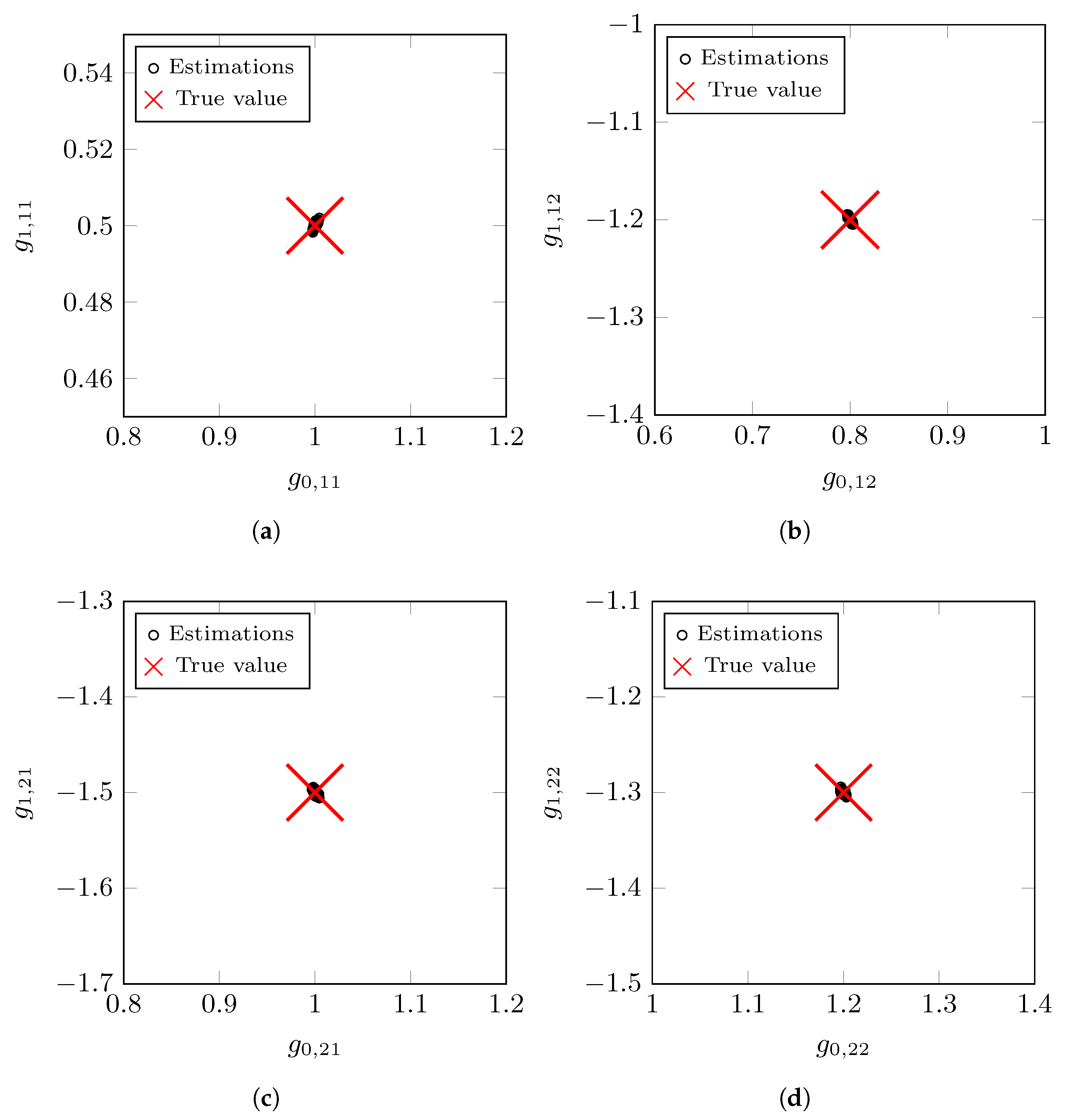
The vector of parameters to be estimated is $\beta ={\left[{\theta }^T{\gamma }^T{\sigma }^2\right]}^T$, with $\theta =\{g_{0,ij},g_{1,ij}\}$, $\gamma ={\{{\alpha }_l,{\mu }_l,{\Sigma }_l\}}_{l=1}^K$, and $K=2$. Figure 4 shows the results of the parameter estimates for the nominal MIMO model $G_0(q^{-1},\eta )$. The large red cross indicates the true value of the parameter vector $\theta$. The black circles represent the estimated nominal model values for all Monte Carlo simulations.

Table 1. Mean values of the estimated parameters of $G_0(q^{-1},\theta )$ and ${\sigma }^2$ for Example 1.

Parameters	${\mathit{g}}_{0,11}$	${\mathit{g}}_{1,11}$	${\mathit{g}}_{0,12}$	${\mathit{g}}_{1,12}$	${\mathit{g}}_{0,21}$	${\mathit{g}}_{1,21}$	${\mathit{g}}_{0,22}$	${\mathit{g}}_{1,22}$	${\mathit{\sigma }}^2$
Estimated values	$0.9873$	$0.5124$	$0.7501$	$-1.1501$	$0.9375$	$-1.4375$	$1.1375$	$-1.2375$	$0.2001$
True values	$1.0$	$0.5$	$0.8$	$-1.2$	$1.0$	$-1.5$	$1.2$	$-1.3$	0.2

presents the mean values of the estimated nominal model parameters and the noise variance across all MC realizations. We observe a small bias in the estimates compared to the true values. This effect can be mitigated by utilizing a larger number of measurements, N, in each independent experiment. The standard deviation of the estimates is similar in each case, with a value close to $\pm 5.1002\times {10}^{-5}$.

Figure 5 shows the estimated multivariate GMM for the distributions of the error-model parameters ${\eta }^{\left[r\right]}$. Figure 5a,b show the estimated GMM for $\{{\eta }_{0,11}^{\left[r\right]},{\eta }_{0,12}^{\left[r\right]}\}$ and $\{{\eta }_{0,21}^{\left[r\right]},{\eta }_{0,22}^{\left[r\right]}\}$, respectively. The Gaussian mixture distributions are drawn utilizing the mean values of the estimated GMM parameters for all MC simulations. We observe the bimodal behavior of the error-model distributions described in (94).

On the other hand, to describe the dynamic behavior using the SE approach, we consider computing the frequency response of the principal gains of the estimated MIMO system model. The principal gains provide a metric to evaluate the estimated MIMO system model performance in terms of how, and to what extent, different linear combinations of the input signals are amplified in the outputs signals, as well as the degree of channel coupling [17,51]. Here, we compute the principal gains of M realizations of the MIMO system model given by

$${\widehat{G}}^{\left[r\right]}\left(q^{-1}\right)={\widehat{G}}_0(q^{-1},\widehat{\theta })+{\widehat{G}}_{\Delta }(q^{-1},{\eta }^{\left[r\right]}),$$

(95)

with $r=1,\cdots ,M$, where ${\widehat{G}}_0(q^{-1},\widehat{\theta })$ is the estimated MIMO nominal system model from the estimated values in Table 1, and ${\widehat{G}}_{\Delta }(q^{-1},{\eta }^{\left[r\right]})$ is obtained from M independent realizations of ${\eta }^{\left[r\right]}$ utilizing the GMM in (13) with the mean values of the estimated parameters, $\widehat{\gamma }$, from all MC simulations. In addition, we consider estimating the MIMO system $\widehat{G}(q^{-1},\theta )$ using the NLS [1] algorithm with a second-order FIR multivariable system model. In order to validate the error-model behavior, we consider the data from 25 independent experiments, and we obtain an estimate of a second-order FIR multivariable model for each independent experiment.

Figure 6 shows the magnitude of the principal gains corresponding to the estimated MIMO system model using the SE approach. In Figure 6a, the solid blue line represents the largest principal gain, $\overline{\sigma }\left({\widehat{G}}_0(q^{-1},\widehat{\theta })\right)$, of the estimated nominal MIMO system model. The blue-shaded region corresponds to the area that described the error-model behavior with respect to the largest principal gain. Similarly, in Figure 6b, the red solid line is the smallest principal gain, $\underline{\sigma }\left({\widehat{G}}_0(q^{-1},\widehat{\theta })\right)$, of the estimated MIMO system model. The red-shaded area corresponds to the estimated uncertainty region in which the smallest principal gains of the estimated true MIMO system lie. In both cases, the dotted black lines represent the principal gains computed from the estimated MIMO system models using the NLS algorithm. We observe that the estimated principal gains lie in the shaded regions (blue and red regions) that described the error-model behavior with the SE approach.

5.2. Example 2: Multivariable FIR System Model with Multiplicative Error-Model

In this example, we consider the MIMO system in (1) with a multiplicative error-model (3) as follows:

$$G_{0,ij}(q^{-1},{\theta }_{ij})=g_{0,ij}+g_{1,ij}{q}^{-1},$$

(96)

$$G_{\Delta ,ij}(q^{-1},{\eta }_{ij}^{\left[r\right]})={\eta }_{0,ij}^{\left[r\right]}+{\eta }_{1,ij}^{\left[r\right]}{q}^{-1},$$

(97)

where $i=1,2$ and $j=1,2$, and the true values of the nominal model are $g_{0,11}=1.0$, $g_{1,11}=0.5$, $g_{0,12}=0.8$, $g_{1,12}=-1.2$, $g_{0,21}=1.0$, $g_{1,21}=-1.5$, $g_{0,22}=1.2$, and $g_{1,22}=-1.3$. The input signal corresponds to $u_t^{\left[r\right]}\sim \mathcal{N}(0,{\sigma }_u^2{I}_2)$, ${\sigma }_u^2=10$, and the noise signal is ${\omega }_t^{\left[r\right]}\sim \mathcal{N}(0,{\sigma }^2{I}_2)$, ${\sigma }^2=0.2$. We consider that ${\eta }_{1,ij}^{\left[r\right]}=-{\eta }_{0,ij}^{\left[r\right]}$—i.e., we focus on uncertainties in the MIMO system at high frequencies with ${\eta }^{\left[r\right]}={[{\eta }_{0,11}^{\left[r\right]},{\eta }_{0,12}^{\left[r\right]},{\eta }_{0,21}^{\left[r\right]},{\eta }_{0,22}^{\left[r\right]}]}^T$. Then, the error-model distribution as an overlapped GMM with $K=2$ is given by ${\alpha }_1={\alpha }_2=0.5$ and

$${\mu }_1=\left[\begin{array}{c}-2\\ -2\\ -1\\ -1\end{array}\right],{\mu }_2=\left[\begin{array}{c}2\\ 2\\ 1\\ 1\end{array}\right],{\Sigma }_1={\Sigma }_2=\left[\begin{array}{cccc}1& 0& 0& 0\\ 0& 1& 0& 0\\ 0& 0& 0.5& 0\\ 0& 0& 0& 0.5\end{array}\right].$$

(98)

As in the previous example, the vector of parameters to be estimated is $\beta ={\left[{\theta }^T{\gamma }^T{\sigma }^2\right]}^T$, with $\theta =\{g_{0,ij},g_{1,ij}\}$, $\gamma ={\{{\alpha }_l,{\mu }_l,{\Sigma }_l\}}_{l=1}^K$, and $K=2$. Figure 7 presents the nominal MIMO system model parameter estimates. The large red cross corresponds to the true value of the parameters for the nominal system model. The black circles represent the parameter estimates of the nominal MIMO system model for all MC realizations.

Table 2. Mean values of the estimated parameters of $G_0(q^{-1},\theta )$ and ${\sigma }^2$ for Example 2.

Parameters	${\mathit{g}}_{0,11}$	${\mathit{g}}_{1,11}$	${\mathit{g}}_{0,12}$	${\mathit{g}}_{1,12}$	${\mathit{g}}_{0,21}$	${\mathit{g}}_{1,21}$	${\mathit{g}}_{0,22}$	${\mathit{g}}_{1,22}$	${\mathit{\sigma }}^2$
Estimated values	$1.0002$	$0.5001$	$0.8001$	$-1.1991$	$1.0003$	$-1.5005$	$1.1985$	$-1.3025$	$0.1907$
True values	$1.0$	$0.5$	$0.8$	$-1.2$	$1.0$	$-1.5$	$1.2$	$-1.3$	0.2

summarizes the mean values of the estimated nominal system model parameters and the noise variance. In contrast to the previous example, we observe that the multiplicative error-model approach improves the estimation accuracy, as the dynamic behavior of the nominal model weights the model uncertainty. In this case, the standard deviation of the estimates remains similar, around $\pm 3.02\times {10}^{-4}$.

In Figure 8, the estimated GMM distribution for the error-model parameters ${\eta }^{\left[r\right]}$ is shown. Figure 8a,b show the estimated GMM for $\{{\eta }_{0,11}^{\left[r\right]},{\eta }_{0,12}^{\left[r\right]}\}$, and $\{{\eta }_{0,21}^{\left[r\right]},{\eta }_{0,22}^{\left[r\right]}\}$, respectively. The GMM distributions are computed utilizing the mean values of the estimated GMM parameters for all MC simulations. We observe the overlapped behavior of the multivariate error-model distribution described in (98).

For this example, we compute the principal gains of the M realizations of the MIMO system model

$${\widehat{G}}^{\left[r\right]}\left(q^{-1}\right)={\widehat{G}}_0(q^{-1},\widehat{\theta })+{\widehat{G}}_{\Delta }(q^{-1},{\eta }^{\left[r\right]}){\widehat{G}}_0(q^{-1},\widehat{\theta }),$$

(99)

with $r=1,\cdots ,M$, where ${\widehat{G}}_0(q^{-1},\widehat{\theta })$ is the estimated MIMO nominal system model where $\widehat{\theta }$ is given by the estimated values in Table 2, and ${\widehat{G}}_{\Delta }(q^{-1},{\eta }^{\left[r\right]})$ is obtained from M independent realizations of ${\eta }^{\left[r\right]}$ utilizing the GMM in (13) with the mean values of the estimated parameters, $\widehat{\gamma }$, from all MC realizations. We also estimate the system $G^{\left[r\right]}(q^{-1},\theta )$ using the NLS [1] algorithm with a second-order FIR multivariable system model. We consider the data from 25 independent experiments and we obtain an estimate of a second-order FIR multivariable model for each independent experiment in order to validate the uncertainty dynamic behavior.

Figure 9a,b show the magnitude of both the largest and smallest principal gains corresponding to the estimated MIMO system model. The solid blue and red lines represent the largest and smallest principal gains computed from the estimated nominal MIMO system model, i.e., $\overline{\sigma }\left({\widehat{G}}_0(q^{-1},\widehat{\theta })\right)$ and $\underline{\sigma }\left({\widehat{G}}_0(q^{-1},\widehat{\theta })\right)$, respectively. The shaded regions (blue and red) correspond to the error-model region in which the principal gains of the true system lie. We observe that all principal gains from the estimated MIMO system using the NLS algorithm (black dotted lines) lie in the error-model area, that is, the estimations lie in the uncertainty region described with the SE approach.

5.3. Example 3: A General MIMO System with Non-Gaussian Mixture Error-Model Distribution

In this example, we consider the MIMO system model in (1) with uncertainties in the parameters of the system model as follows:

$$G_{ij}^{\left[r\right]}\left(q^{-1}\right)={\displaystyle \frac{b_{1,ij}^{\left[r\right]}{q}^{-1}}{1+a_{1,ij}^{\left[r\right]}{q}^{-1}}},$$

(100)

where $i=1,2$, $j=1,2$, $u_t^{\left[r\right]}\sim \mathcal{N}(0,{\sigma }_u^2{I}_2)$, ${\sigma }_u^2=10$, and ${\omega }_t^{\left[r\right]}\sim \mathcal{N}(0,{\sigma }^2{I}_2)$, ${\sigma }^2=0.2$. The parameters $b_{1,ij}^{\left[r\right]}$ and $a_{1,ij}^{\left[r\right]}$ are given by

$$b_{1,ij}=b_{1,ij}^o(1+{\delta }_{ij}^{\left[r\right]}),a_{1,ij}=a_{1,ij}^o(1+{\delta }_{ij}^{\left[r\right]}),$$

(101)

where $b_{1,11}^o=1.0$, $a_{1,11}^o=-0.3$, $b_{1,12}^o=0.8$, $a_{1,12}^o=-0.4$, $b_{1,21}^o=1.1$, $a_{1,21}^o=-0.5$, $b_{1,22}^o=1.0$, $a_{1,22}^o=-0.6$, and ${\delta }_{ij}^{\left[r\right]}$ is uniformly distributed as $\mathcal{U}[-0.2,0.2]$.

In the SE framework, we consider a multiplicative error-model and a nominal MIMO system model as follows:

$$G_{0,ij}(q^{-1},\theta )={\displaystyle \frac{b_{1,ij}{q}^{-1}}{1+a_{1,ij}{q}^{-1}}},$$

(102)

$$G_{\Delta ,ij}(q^{-1},{\eta }_{ij}^{\left[r\right]})={\eta }_{0,ij}^{\left[r\right]}+{\eta }_{1,ij}^{\left[r\right]}{q}^{-1},$$

(103)

where $\theta =\{b_{1,ij},a_{1,ij}\}$, $i=1,2$, and $j=1,2$. The distribution of the parameters ${\eta }^{\left[r\right]}=\{{\eta }_{0,ij}^{\left[r\right]},{\eta }_{1,ij}^{\left[r\right]}\}$ of the error-model in (103) is considered a GMM with $K=2$—that is, $\gamma ={\{{\alpha }_l,{\mu }_l,{\Sigma }_l\}}_{l=1}^K$. The vector of parameters to be estimated is $\beta =\left[{\theta }^T{\gamma }^T{\sigma }^2\right]$. In this case, the advantage of the proposed algorithm lies in the fact that a non-Gaussian PDF can be accurately approximated by a linear combination of Gaussian distributions [65]. Gaussian mixture approximations enhance the accuracy of the estimates when Gaussian assumptions are relaxed (see, e.g., [6,35]).

In order to validate proposed SE approach for the MIMO system in (100), we compute the principal gains of M independent realizations of the vector of parameters ${\eta }^{\left[r\right]}$ in (99) with $r=1,\cdots ,M$. The vector of parameters $\widehat{\theta }$ corresponds to the average of the estimated parameters of the nominal MIMO system model for all MC simulations. The vector of parameters ${\eta }^{\left[r\right]}$ is computed from a GMM as in (13) using the average of the estimated Gaussian mixture parameters from the MC simulations. In addition, we estimate the MIMO system model $\widehat{G}(q^{-1},\theta )$ with the system model structure in (102) using the NLS algorithm. In particular, we use the measurements of 25 independent experiments and we estimate $\widehat{G}(q^{-1},\theta )$ for each experiment, that is, for $r=1,\cdots ,25$.

Figure 10a,b show the frequency response of the largest and the smallest principal gains, respectively, for the estimated MIMO system model with the SE approach. The solid blue and red lines represent the largest and smallest principal gain of the estimated nominal MIMO system model, ${\widehat{G}}_0(q^{-1},\widehat{\theta })$. The two shaded areas are the uncertainty regions in which the principal gains computed from the M realizations of ${\eta }^{\left[r\right]}$ in (99) lie. The dotted black lines represent the principal gains of the estimated MIMO system models using the NLS algorithm. We observe that the principal gains from the estimated MIMO system $\widehat{G}(q^{-1},\theta )$ lie in the uncertainty regions despite the fact that the SE system model in (99) does not correspond to the system model structure in (102).

Remark 3. 

In the numerical simulations, we consider that the MIMO system model structure (both nominal model and error-model), and the number of components, K, of the GMM are known. However, we can use an information criterion, e.g., Akaike’s information criterion [66], in order to obtain a candidate reduced complexity model that explains the dynamic behavior with good accuracy from a set of system models in which the true system model does not lie; see, e.g., [67].

6. Conclusions

In this paper, we addressed the problem of modeling parametric and structural uncertainties in a class of MIMO linear dynamic systems using the SE approach. We considered that the MIMO system model was a realization drawn from an underlying probability space, and its dynamic behavior was described by combining a deterministic nominal model and a stochastic error-model with a non-Gaussian PDF as a GMM. We formulated an ML estimation algorithm in which the error-model parameters were treated as hidden variables to obtain estimates of the vector of parameters that define both the MIMO nominal system model and the multivariate GMM parameters. In this context, we used the combined information from a set of independent experiment measurements, obtaining the likelihood function as an infinite mixture distribution and marginalizing with respect to the hidden variables for both the additive error model and the multiplicative error model cases. We proposed an iterative EM-based algorithm to solve the corresponding ML estimation problem, yielding closed-form expressions for the estimators of the GMM parameters and the noise variance. Estimating the nominal MIMO system model parameters was also addressed utilizing a gradient descent methodology. The simulation results demonstrated accurate estimates of the nominal MIMO system model and a good description of the uncertainty region, including a scenario where there exist non-Gaussian parametric uncertainties that did not correspond to a GMM and where the true system model did not correspond to the SE system model assumption. As future work, this multivariable SE approach can be extended in applications of hybrid systems which exhibit both continuous time dynamics and discrete switching behavior using sampled data or in scenarios where system model parameters are intrinsically discrete, e.g., logical conditions or classification labels, to mention a few.