Article

Prioritized Decision Support System for Cybersecurity Selection Based on Extended Symmetrical Linear Diophantine Fuzzy Hamacher Aggregation Operators

by
Muhammad Zeeshan Hanif
* and
Naveed Yaqoob
Department of Mathematics and Statistics, Riphah International University, I-14, Islamabad 44000, Pakistan
*
Author to whom correspondence should be addressed.
Symmetry 2025, 17(1), 70; https://doi.org/10.3390/sym17010070
Submission received: 30 September 2024 / Revised: 23 December 2024 / Accepted: 26 December 2024 / Published: 3 January 2025
(This article belongs to the Special Issue Recent Developments on Fuzzy Sets Extensions)

Abstract

:
The symmetrical linear Diophantine fuzzy Hamacher aggregation operators play a fundamental role in many decision-making applications. The selection of a cyber security system is of paramount importance for maintaining digital assets. It necessitates a comprehensive review of threat landscapes, vulnerability assessments, and the specific needs of the organization in order to ensure the implementation of effective security measures. Smart grid (SG) technology uses modern communication and monitoring technologies to enhance the management and regulation of electricity production and transmission. However, greater dependence on technology and connection creates new vulnerabilities, exposing SG communication networks to large-scale attacks. Unlike previous surveys, which often give broad overviews of SG design, our research goes a step further, giving a full architectural layout that includes major SG components and communication linkages. This in-depth review improves comprehension of possible cyber threats and allows SGs to analyze cyber risks more systematically. To determine the best cybersecurity strategies, this study introduces a multi-criteria group decision-making (MCGDM) approach using the linear Diophantine fuzzy Hamacher prioritized aggregation operator (LDFHPAO). In real-world applications, aggregation operators (AOs) are essential for information fusion. This research presents innovative prioritized AOs designed to address MCGDM problems in uncertain environments. We developed the LDF Hamacher prioritized weighted average (LDFHPWA) and LDF Hamacher prioritized weighted geometric (LDFHPWG) operators, which address the shortcomings of traditional operators and provide a more robust modeling approach for MCGDM challenges. This study also outlines key characteristics of these new prioritized AOs. An MCGDM approach incorporating these operators is proposed and demonstrated to be effective through an example that compares and selects the optimal cybersecurity.

1. Introduction

1.1. Literature Review

The symmetrical linear Diophantine fuzzy Hamacher aggregation operators lead to a new dependable approach to fuzzy decision making. These operators combine linear Diophantine equations with symmetrical properties to efficiently aggregate uncertain information. This leads to more accurate decision-making outcomes in many cases.
In Figure 1, we explain the different types of cyberattacks, including DoS, Insider, Malware, SQL, and related attacks, which can affect data.
The previous generation of power grid is becoming less effective in delivering and distributing electricity owing to the growing issues of integrating renewable energy, handling energy storage, and working with high asset prices. SG technology has emerged as a critical instrument for modernizing and improving present electrical systems in order to overcome existing constraints. By employing modern network communication and monitoring technology, SGs enable effective control of power distribution from a variety of generating sources while adjusting to changes in end user demand. The combination of renewable energy with distributed generation (DG) represents a significant step forward in the construction of an electrical system. Enhanced connectivity and increased reliance on technology introduce new vulnerabilities to cyber threats. Cybercriminals can exploit smart grid communication networks to carry out large-scale attacks, such as Denial-of-Service (DoS) attacks, malware infections, phishing schemes, insider threats, SQL injection attacks, and data manipulation, all targeting these interconnected systems and infrastructure (see Figure 1) [1]. As cyber threats become more complex and widespread, it is crucial to implement robust security measures to safeguard the interconnected power infrastructure. This paper seeks to examine the multiple facets of smart grid cyber and investigate effective strategies for improving security. Many research studies on cybersecurity in smart grids have been conducted, each bringing unique insights and focusing on different components of the smart grid. Woo et al. [2] examined the methodology employed in the assessment of cyber security within the context of the smart grid. Ansari et al. [3] conducted an analysis of the responses to identified cyberattacks within smart distribution systems. Alkuwari et al. [4] elucidated the detection mechanisms within smart grids and presented a comprehensive survey from the standpoint of cybersecurity. Liu et al. [5] conducted a comprehensive review of the principles governing learning-based intrusion detection systems and their potential applications within smart grids. Alwageed [6] examined the identification of cyberattacks within smart grids through the application of machine learning models. Zhai et al. [7] conducted an analysis of algorithms designed for privacy-preserving outsourcing in the context of multidimensional data encryption within smart grids. Miller et al. [8] examined the impact of human factors within the context of the smart grid system of systems demand response. Fredman [9] explored the human dimensions of the smart grid, focusing on behavior-driven energy efficiency among renters through the utilization of real-time feedback and competitive, performance-oriented incentives. Montañez et al. [10] investigated human cognition in the context of social engineering cyberattacks. Ray [11] conducted training programs aimed at enhancing cybersecurity awareness and ensuring compliance within non-profit organizations. Loi and Christen [12] examined the ethical frameworks pertinent to cybersecurity. Rahman et al. [13] examined the methodologies for ensuring secure and private data aggregation in the context of energy consumption scheduling within smart grids. Albasrawi et al. [14] performed an analysis on the reliability and resilience of smart grids. Kanca et al. [15] highlighted the importance of sharing cyber threat intelligence and fostering collaboration.
Decision making (DM) is crucial in daily life, involving a process where all options are evaluated based on the decision makers’ assessment data, leading to the selection of the most suitable choice. Historically, decision makers relied on real numbers to provide their assessments. As multi-attribute decision-making (MADM) [16,17] scenarios have become increasingly complex, experts are struggling to provide accurate numerical assessments of options. The inherent uncertainties and imprecisions in human judgment have exposed the limitations of the traditional crisp set theory. Therefore, Zadeh [18] established the foundational theory of Fuzzy sets (FSs) to help address uncertainty in knowledge by letting experts express their level of satisfaction (membership degree) with a member’s performance, within a range from 0 to 1. While fuzzy sets offer a basis for handling uncertain assessments, they are insufficient for no-membership degree (NMD). To address the limitations of FS, Atanassov [19] introduced intuitionistic fuzzy sets (IFSs), which incorporate both MD and NMD. This dual approach makes IFSs more effective and versatile compared to traditional FSs. IFSs allow for a larger degree of ambiguity in DM by providing information about possible choices in both MD and NMD. However, the Atanassov model contains a restriction: 0 ≤ MD + NMD ≤ 1. For example, consider a scenario where the MD of a particular element within a set is 0.7, and the NMD is 0.6. When the sum of these two values is computed, it exceeds 1, thereby revealing a significant limitation in the model’s ability to accurately capture the data’s characteristics. To address such challenges, Yager [20] pioneered the idea of Pythagorean fuzzy sets (PFSs), which offer greater flexible conditions that allow for efficient handling of imprecise decisions. Despite their advantages, PFSs have limitations. For example, if an element’s MD is 0.8 and NMD is 0.7, their squared sum is greater than 1. In response, Yager [21] developed q-rung orthopair fuzzy sets (q-ROFSs), which limit the total of MD and NMD’s qth powers to a maximum of one. q-ROFSs outperform IFSs and PFSs in managing both vagueness and overlooked data. The knowledge, similarity, dissimilarity, and divergence measures of q-ROFSs are explored in references [22,23,24]. The idea of LDFSs was first presented by Riaz and Hashmi [25]. In many uncertain real-world situations, relying solely on the MD and NMD is insufficient for analyzing objects or alternatives. To enhance this analysis, additional assessments are needed beyond MD and NMD. Linear Diophantine fuzzy numbers (LDFNs) incorporate reference parameters (RPs) that provide extra layers of ranking based on the decision maker’s preferences. This approach improves the efficiency and reliability of the decision-making process. The inclusion of RPs in the LDFS technique makes it more adaptable and effective compared to other methods. LDFSs, which are widely used in various academic fields [26,27,28,29], expand the traditional MD and NMD framework by addressing gaps and integrating RPs. This method offers two layers of data, each constrained by a specific parameter, and allows for combinations of RPs with MD and NMD. MCGDM is the process of choosing the best option from a set of alternatives by evaluating them against a defined set of criteria. Various AOs are utilized for solving problems involving many criterion groups. The first method uses several AOs. Hamacher, Einstein, and Dombi are examples of average and geometric operators, among others. Traditional approaches provide simply ratings. When using AOs, all alternatives are examined and ranked. It is more reasonable to examine the alternatives completely, taking into account the weights assigned to the qualities. Xu and Yager [30] proposed the IFSs for some algebraic AOs. Xu [30] proposed some geometric AOs under IFSs. Hamacher operations [31], specifically the Hamacher T-norm (TN) and T-conorm (TCN), are powerful alternatives to algebraic multiplication and summation. Many researchers have investigated Hamacher AOs and their applications to MCGDM issues [32,33]. Huang [34] defined Hamacher aggregation for IFSs. Wu [35] defined the Hamacher aggregation operator for PFSs. Darko et al. [36] suggested Hamacher AOs for q-ROFs. Shams et al. [37] defined Hamacher AOs non-LDFSs. Liu [32] employed Hamacher aggregation operations in IVIFNs and talked about MAGDM approaches. Einstein hybrid aggregation operations for IFNs were proposed by Zhang et al. [38]. The Hamacher TN and TCN are an extension of the Einstein TN and TCN [39] but are more universal and flexible. Seikh et al. [40] proposed Dombi AOs for IFSs. Akram et al. [41] presented Dombi AOs for PFS.s Dombi AOs and the TOPSIS method for FFSs were proposed by Aydemir et al. [42]. Assuming the attribute’s priority level, all of the aforementioned operators have the same type. Yager [43] introduced many prioritized AOs. Yager suggested that economic considerations should not restrict the efficacy of protection, particularly when selecting a child’s cycle based on protection and affordability. An aggregation problem arises due to the priority relationship between these criteria, with protection being the first priority. To address this, AOs like average and geometric operators are used, considering higher priority criteria when safety is not feasible. IF prioritized weighted average (IFPWA) and weighted geometric (IFPWG) operators were proposed by Yu [44] to address the problem of attribute prioritization in an intuitionistic fuzzy environment; these were then applied to MADM problems. IF Einstein prioritized weighted average (IFEPWA) and weighted geometric (IFEPWG) operators were proposed by Verma and Sharma [45]. Prioritized averaging and geometric AOs for the IF soft set environment were proposed by Arora and Garg [46]. Khan et al. [47] proposed prioritized AOs for PFSs. Gao and Hui [48] proposed Hamacher prioritized AOs for PFSs. Hamacher prioritized AOs for FFSs were proposed by Jan et al. [49]. Akram et al. [50] suggested prioritized weighted AOs for complex spherical fuzzy environments. Riaz et al. [51] proposed prioritized aggregation operators for LDFSs. Riaz et al. [52] proposed Einstein prioritized aggregation operators for LDFSs. From the aforementioned literature on decision-making scenarios, it could be observed that the criteria and the individuals accountable for making decisions frequently exhibit varying degrees of priority. The prioritization of criteria significantly influences the selection of operators within the decision-making framework. Consequently, the application of uniform priority levels to both criteria and decision makers may occasionally result in complications. In addressing this challenge, we opted to implement prioritized alternative operators (AOs) within linear Diophantine fuzzy sets (LDFSs), as they serve to mitigate these issues.

1.2. Contribution and Novelty

The LDFS theory addresses the limitations of IFSs, PFSs, and q-ROFs in evaluating MD and NMD, making it difficult for decision makers to fully explore alternatives. By implementing a system that allows decision makers to choose grades ranging from 0 to 1, reference parameters can be employed to form intersections and unions. Additionally, using Hamacher sums and products provides a smoother approximation compared to algebraic sums and products. When a priority relationship exists among criteria, the recommended AOs can be effectively applied. The LDFS theory is a valuable tool for combining prioritized AOs and Hamacher AOs to develop prioritized Hamacher AOs, which can incorporate prioritization among attributes or decision makers, which is essential for real-world DM scenarios. For example, in selecting cybersecurity options based on criteria such as security effectiveness, cost-effectiveness, network segmentation, threat intelligence, and patch management, security effectiveness might be prioritized. The usefulness and validity of the suggested method are demonstrated by comparing it to existing methodologies and AOs.
This article highlights its key contributions and innovations as follows:
  • LDFS is a flexible method that overcomes MD and NMD limitations in existing models like IFSs, PFSs, and q-ROFSs. It allows decision makers to select grades within the [0, 1] range and utilize reference or control characteristics as weight vectors, facilitating the classification of physical attributes and the handling of ambiguous data.
  • Hamacher AOs are utilized to facilitate seamless information integration while prioritized operators connect various criteria according to their importance. To maximize the potential of these operators, we are developing new hybrid AOs.
  • We suggest two hybrid AOs to mitigate the effects of extremely large or small values in DM on overall rankings. These are the LDFHPWA and LDFHPWG operators.
  • Several appealing aspects of the suggested AOs are also examined, including boundary conditions, idempotence, and monotonicity.
  • A new DM approach utilizing the proposed operators is introduced to address MCDM problems.
  • A novel DM method incorporating the proposed operators is introduced to tackle MCDM challenges.

1.3. Motivation for This Research

In various DM situations, criteria and decision makers often have different levels of priority. The way criteria are prioritized affects the choice of operators in the decision-making process. Thus, applying uniform priority levels to both criteria and DMs can sometimes lead to issues. To overcome this challenge, we decided to use prioritized alternative operators (AOs) within linear Diophantine fuzzy sets (LDFSs), as they help alleviate these problems.
The paper is structured in the following manner: Section 2 briefly explains several key concepts related to LDFSs. Section 3 introduces the Hamacher prioritized AOs, including the LDFHPWA and LDFHPWG aggregation operators. Section 4 investigates the solution for the MCGDM issue that uses Hamacher prioritized AOs. Section 5 develop presents a case study focusing on the selection of cybersecurity options. Section 6 provides a summary of the article’s conclusions and suggests potential directions for future research.

2. Preliminaries

This subsection explains the notions of the IFS, PFS, q-ROFS, and LDFS. Unless suggested differently, the set Y = y 1 ,   y 2 , , y n corresponds to the universal set.
Definition 1
([21]). Consider a fixed set  Y ; an IFS is defined as follows:
Ɠ = y j ,   ɧ Ɠ y j , Ӵ Ɠ   y j   | y j     Y .
Here,  ɧ Ɠ y j  and  Ӵ Ɠ   y j  are the MD and NMD of  y j   Y , respectively, with  ɧ Ɠ y j , Ӵ Ɠ   y j 0 ,   1  and  0 ɧ Ɠ y j + Ӵ Ɠ   y j 1 . For  y j   Y , the level of indeterminacy is characterized by  π ¯ A = 1 ɧ Ɠ y j Ӵ Ɠ   y j .
Here Equation (1) represents the set of pair of values corresponding to Y and the level of indeterminacy.
Definition 2
([25]). Consider a fixed set  Y ; an IFS is defined as follows:
Ԣ = y j ,   ɧ Ԣ y j , Ӵ Ԣ   y j   | y j     Y  
Here,  ɧ Ԣ y j  and  Ӵ Ԣ   y j  are the MD and NMD of  y j   Y , respectively, with  ɧ Ԣ y j , Ӵ Ԣ   y j 0 ,   1  and  0   ɧ Ԣ y j 2 + Ӵ Ԣ   y j 2 1 . For  y j   Y , the level of indeterminacy is characterized by  π ¯ Ԣ = 1   ɧ Ԣ y j 2 Ӵ Ԣ   y j 2 .
Equation (2) depicts the IFS in relation to the Pythagorean condition on Y and the level of indeterminacy.
Definition 3
([30]). Consider a fixed set  Y ; an IFS is defined as follows:
= y j ,   ɧ y j , Ӵ   y j   | y j     Y .  
Here,  ɧ y j  and  Ӵ   y j  are the MD and NMD of  y j   Y , respectively, with  ɧ y j , Ӵ   y j 0 ,   1  and  0   ɧ y j q + Ӵ   y j q 1 . For  y j   Y , the level of indeterminacy is characterized by  π ¯ Ԣ = 1   ɧ y j q Ӵ   y j q q .
In Equation (3) depicts the IFS in relation to the MD and NMD on Y and the level of indeterminacy.

2.1. Linear Diophantine Fuzzy Set (LDFS)

Definition 4
([35]). Consider a fixed set  Y ; an IFS is defined as follows:
Ƣ = y j ,   ɧ Ƣ y j , Ӵ Ƣ   y j , E , : y j     Y ,  
where  ɧ Ƣ y j , Ӵ Ƣ   y j , E , 0 ,   1  are the MD, NMD, and RPs, respectively, of  y j   Y  respectively, and hold the condition  0 E ɧ Ƣ y j + Ӵ Ƣ   y j 1 , with  0 E + 1 . Such RPs may help with the description or identification of a specific system. The indeterminacy degree is specifically defined as  π ¯ Ƣ = 1 E ɧ Ƣ y j Ӵ Ƣ   y j . The RPs associated with the indeterminacy degree are denoted as ẞ.
The following graphs demonstrate that q-ROFSs provide DMs with additional room to evaluate any option. We present a visual representation of an LDFS with various RP combinations and demonstrate that its measurement space is greater than IFS and PFS. Figure 2 compares an IFS, PFS, and q-ROFFS, whereas Figure 3, Figure 4, Figure 5 and Figure 6 depict the graphical representation of LDFSs with various pairings of constant RPs.

2.2. Expectation Score Function

Definition 5
([52]). If  Ƣ = ɧ Ƣ , Ӵ Ƣ   , E ,  is a nNon-LDFN, the expectation score function may be given by the mapping  : N o n L D F N ( U ) 0 ,   1  and provided as:
Տ ̿ = 1 4 ɧ Ƣ Ӵ Ƣ + 1 + 1 4 E + 1 ,      
where  L D F N ( U )  is a collection of LDFNs on U.

2.3. Hamacher Operations

Hamacher [31] suggested Hamacher operations, a generalized variant of TN and TCN that includes the Hamacher product and sum. These are the concepts for the well-known TN and TCN, as defined below.
Definition 6
(Hamacher [31]). Assume  ʆ ~  and  ɸ ~  are two real numbers. Then, Hamacher TN and TCN are defined as:
ʆ ~ , ɸ ~ = ʆ ~ H ɸ ~ = ʆ ~ + ɸ ~ ʆ ~ ɸ ~ 1 Ք ~ ʆ ~ ɸ ~ 1 1 Ք ~ Ⱥ ~ Ȼ ~ ,       Ք ~ > 0 ,  
* ʆ ~ , ɸ ~ = ʆ ~ H ɸ ~ = ʆ ~ ɸ ~ Ք ~ + 1 Ք ~ ʆ ~ + ɸ ~ ʆ ~ ɸ ~ ,       Ք ~ > 0 .    
Particularly, if  l = 1 , then Hamacher TN and TCN are simplified to algebraic TN and TCN, as follows:
ʆ ~ , ɸ ~ = ʆ ~ H ɸ ~ = ʆ ~ + ɸ ~ ʆ ~ ɸ ~ ,  
* ʆ ~ , ɸ ~ = ʆ ~ H ɸ ~ = ʆ ~ ɸ ~ .  
Particularly, if  l = 2 , then Hamacher TN and TCN are simplified to Einstein TN and TCN, as follows:
      ʆ ~ , ɸ ~ = ʆ ~ H ɸ ~ = ʆ ~ + ɸ ~ 1 + ʆ ~ ɸ ~ ,  
* ʆ ~ , ɸ ~ = ʆ ~ H ɸ ~ = ʆ ~ ɸ ~ 1 + 1 ʆ ~ 1 ɸ ~   .

2.4. The Operational Laws for LDFNs Based on Hamacher Operations

In this section, we describe Hamacher operations in relation to LDFNs based on Hamacher TN and TCN.
Definition 7
([48]). If  Ƣ 1 = ɧ Ƣ 1 , Ӵ Ƣ 1 , E 1 , 1  and  Ƣ 2 = ɧ Ƣ 2 , Ӵ Ƣ 2 , E 2 , 2  are any two LDFNs, where  α 0 ,   1  and  Ք ~ 1  are real numbers. Then Hamacher TN and TCN operations of FFLNs are defined as:
  • Ƣ 1 H Ƣ 2 = ɧ Ƣ 1 + ɧ Ƣ 2 ɧ Ƣ 1 ɧ Ƣ 2   1 Ք ~ ɧ Ƣ 1 ɧ Ƣ 2 1   1 Ք ~ ɧ Ƣ 1 ɧ Ƣ 2   , Ӵ Ƣ 1 Ӵ Ƣ 2 Ք ~ +   1 Ք ~ Ӵ Ƣ 1 + Ӵ Ƣ 2 Ӵ Ƣ 1 Ӵ Ƣ 2 , E 1 + E 2 E 1 E 2 1 Ք ~ E 1 E 2 1   1 Ք ~ E 1 E 2   , 1 2 Ք ~ +   1 Ք ~ 1 + 2 1 2 ;
  • Ƣ 1 H Ƣ 2 = ɧ Ƣ 1 ɧ Ƣ 2 Ք ~ +   1 Ք ~ ɧ Ƣ 1 + ɧ Ƣ 2 ɧ Ƣ 1 ɧ Ƣ 2   , Ӵ Ƣ 1 + Ӵ Ƣ 2 Ӵ Ƣ 1 Ӵ Ƣ 2 1 Ք ~ Ӵ Ƣ 1 Ӵ Ƣ 2 1   1 Ք ~ Ӵ Ƣ 1 Ӵ Ƣ 2 , E 1 E 2 Ք ~ +   1 Ք ~ E 1 + E 2 E 1 E 2   , 1 + 2 1 2   1 Ք ~ 1 2 1   1 Ք ~ 1 2 ;
  • α H Ƣ 1 = 1 + Ք ~ 1 ɧ Ƣ 1 α 1 ɧ Ƣ 1 α 1 + Ք ~ 1 ɧ Ƣ 1 α + Ք ~ 1 1 ɧ Ƣ 1 α   , Ք ~ Ӵ Ƣ 1 α 1 + Ք ~ 1 1 Ӵ Ƣ 1 α + Ք ~ 1 Ӵ Ƣ 1 α , 1 + Ք ~ 1 E 1 α 1 E 1 α 1 + Ք ~ 1 E 1 α + Ք ~ 1 1 E 1 α   , Ք ~ 1 α 1 + Ք ~ 1 1 1 α + Ք ~ 1 1 α ;
  • Ƣ 1 α = Ք ~ ɧ Ƣ 1 α 1 + Ք ~ 1 1 ɧ Ƣ 1 α + Ք ~ 1 ɧ Ƣ 1 α   , 1 + Ք ~ 1 Ӵ Ƣ 1 α 1 Ӵ Ƣ 1 α 1 + Ք ~ 1 Ӵ Ƣ 1 α + Ք ~ 1 1 Ӵ Ƣ 1 α , Ք ~ E 1 α 1 + Ք ~ 1 1 E 1 α + Ք ~ 1 E 1 α   , 1 + Ք ~ 1 1 α 1 1 α 1 + Ք ~ 1 1 α + Ք ~ 1 1 1 α .

3. Linear Diophantine Fuzzy Hamacher Prioritized Aggregation Operators

In this part, we discuss the LDF Hamacher prioritized weighted average (LDFHPWA) and LDF Hamacher prioritized weighted geometric (LDFHPWG) operators. We next go over certain desired features in detail, including idempotency, monotonicity, and boundedness. In 2008, Yager [43] developed the notion of Prioritized Average (PA), as defined below:
Definition 8.
Let  = 1 , 2 , , n ¯  be a set of parameters with a prioritization established based on the linear ordering of the criteria of  1 , 2 , , n ¯ . If  b _ > k , clearly explain that parameter  b _  has a greater priority than  k  and  n N .  The real number  b _ x 0 ,   1  represents the performance of any option according to the criterion  b _ .
P A a _ = b _ = 1 q _ Θ b _ b _ x ,    
where  Θ b _ = ψ ^ b _ b _ = 1 q _ ψ ^ b _ ,   ψ ^ b _ = l = 1 b _ 1 k x   b _ = 2,3 , n ¯   ,   ψ ^ 1 = 1 . The prioritized average (PA) operator is then introduced as  b _ q _ = X ~ b _ .

3.1. LDF Hamacher Prioritized Weighted Average (LDFHPWA) Operator

Definition 9.
Let  Ƣ b _ = ɧ Ƣ b _ , Ӵ Ƣ b _ , E b _ , b _ b _ = 1,2 , 3 , , q _  be a set of LDFNs. Then, the LDF Hamacher prioritized weighted average (LDFHPWA) operator is the function  L D F H P W A : Ƣ q _ Ƣ ,  such that:
L D F H P W A Ƣ 1 ,   Ƣ 2 , , Ƣ q _ = b _ = 1 q _ ψ ^ b _ X ~ b _ ψ ^ b _ Ƣ b _                                                 = ψ ^ 1 _ X ~ b _ ψ ^ b _ Ƣ 1 ψ ^ 2 _ X ~ b _ ψ ^ b _ Ƣ 2 ψ ^ q _ X ~ b _ ψ ^ b _ Ƣ b _ ,  
where  ψ ^ j _ = l = 1 j _ 1 Տ ̿ Ƣ l ,   j _ = 2 ,   3 , ,   n ¯ ,   ψ ^ 1 = 1 , and  Տ ̿ Ƣ l  is the score of LDFNs  Ƣ l = ɧ Ƣ l , Ӵ Ƣ l , E l , l .
Theorem 1.
Let  Ƣ b _ = ɧ Ƣ b _ , Ӵ Ƣ b _ , E b _ , b _ b _ = 1,2 , 3 , , q _  be a set of LDFNs. When these LDFNs are aggregated using the LDFHPWA operation, the resulting value is also an LDFN.
L D F H P W A Ƣ 1 ,   Ƣ 2 , , Ƣ q _ = ψ ^ 1 _ X ~ b _ ψ ^ b _ Ƣ 1 ψ ^ 2 _ X ~ b _ ψ ^ b _ Ƣ 2 ψ ^ q _ X ~ b _ ψ ^ b _ Ƣ b _ = b _ = 1 q _ 1 + Ք ~ 1 ɧ Ƣ b _ ψ ^ b _ X ~ b _ ψ ^ b _ b _ = 1 q _ 1 ɧ Ƣ b _ ψ ^ b _ X ~ b _ ψ ^ b _ b _ = 1 q _ 1 + Ք ~ 1 ɧ Ƣ b _ ψ ^ b _ X ~ b _ ψ ^ b _ + Ք ~ 1 b _ = 1 q _ 1 ɧ Ƣ b _ ψ ^ b _ X ~ b _ ψ ^ b _   , Ք ~ b _ = 1 q _ Ӵ Ƣ b _ ψ ^ b _ X ~ b _ ψ ^ b _ b _ = 1 q _ 1 + Ք ~ 1 1 Ӵ Ƣ b _ ψ ^ b _ X ~ b _ ψ ^ b _ + Ք ~ 1 b _ = 1 q _ Ӵ Ƣ b _ ψ ^ b _ X ~ b _ ψ ^ b _ , b _ = 1 q _ 1 + Ք ~ 1 E b _ ψ ^ b _ X ~ b _ ψ ^ b _ b _ = 1 q _ 1 E b _ ψ ^ b _ X ~ b _ ψ ^ b _ b _ = 1 q _ 1 + Ք ~ 1 E b _ ψ ^ b _ X ~ b _ ψ ^ b _ + Ք ~ 1 b _ = 1 q _ 1 E b _ ψ ^ b _ X ~ b _ ψ ^ b _   , Ք ~ b _ = 1 q _ b _ ψ ^ b _ X ~ b _ ψ ^ b _ b _ = 1 q _ 1 + Ք ~ 1 1 b _ ψ ^ b _ X ~ b _ ψ ^ b _ + Ք ~ 1 b _ = 1 q _ b _ ψ ^ b _ X ~ b _ ψ ^ b _
where,  ψ ^ b _ = l = 1 j _ 1 Տ ̿ Ƣ l ,   b _ = 2 ,   3 , ,   q _ ,   ψ ^ 1 = 1 , and  Տ ̿ Ƣ l  is the score of LDFNs  Ƣ l = ɧ Ƣ l , Ӵ Ƣ l , E l , l .
Proof: 
Use mathematical induction for proof. For q _ = 1
ψ ^ 1 X ~ b _ ψ ^ b _ Ƣ 1 = 1 + Ք ~ 1 ɧ Ƣ 1 ψ ^ 1 X ~ b _ ψ ^ b _ 1 ɧ Ƣ 1 ψ ^ 1 X ~ b _ ψ ^ b _ 1 + Ք ~ 1 ɧ Ƣ 1 ψ ^ 1 X ~ b _ ψ ^ b _ + Ք ~ 1 1 ɧ Ƣ 1 ψ ^ 1 X ~ b _ ψ ^ b _   , Ք ~ Ӵ Ƣ 1 ψ ^ 1 X ~ b _ ψ ^ b _ 1 + Ք ~ 1 1 Ӵ Ƣ 1 ψ ^ 1 X ~ b _ ψ ^ b _ + Ք ~ 1 Ӵ Ƣ 1 ψ ^ 1 X ~ b _ ψ ^ b _ , 1 + Ք ~ 1 E 1 ψ ^ 1 X ~ b _ ψ ^ b _ 1 E 1 ψ ^ 1 X ~ b _ ψ ^ b _ 1 + Ք ~ 1 E 1 ψ ^ 1 X ~ b _ ψ ^ b _ + Ք ~ 1 1 E 1 ψ ^ 1 X ~ b _ ψ ^ b _   , Ք ~ 1 ψ ^ 1 X ~ b _ ψ ^ b _ 1 + Ք ~ 1 1 1 ψ ^ 1 X ~ b _ ψ ^ b _ + Ք ~ 1 1 ψ ^ 1 X ~ b _ ψ ^ b _ = ɧ Ƣ 1 , Ӵ Ƣ 1 , E 1 , 1 .
Therefore, Equation (14) is true for q _ = 1 . Suppose Equation (14) is true for q _ = v _ .
L D F H P W A Ƣ 1 ,   Ƣ 2 , , Ƣ v _ = ψ ^ 1 _ X ~ b _ ψ ^ b _ Ƣ 1 ψ ^ 2 _ X ~ b _ ψ ^ b _ Ƣ 2 ψ ^ v _ X ~ b _ ψ ^ b _ Ƣ v _ = b _ = 1 v _ 1 + Ք ~ 1 ɧ Ƣ b _ ψ ^ b _ X ~ b _ ψ ^ b _ b _ = 1 v _ 1 ɧ Ƣ b _ ψ ^ b _ X ~ b _ ψ ^ b _ b _ = 1 v _ 1 + Ք ~ 1 ɧ Ƣ b _ ψ ^ b _ X ~ b _ ψ ^ b _ + Ք ~ 1 b _ = 1 v _ 1 ɧ Ƣ b _ ψ ^ b _ X ~ b _ ψ ^ b _   , Ք ~ b _ = 1 v _ Ӵ Ƣ b _ ψ ^ b _ X ~ b _ ψ ^ b _ b _ = 1 v _ 1 + Ք ~ 1 1 Ӵ Ƣ b _ ψ ^ b _ X ~ b _ ψ ^ b _ + Ք ~ 1 b _ = 1 v _ Ӵ Ƣ b _ ψ ^ b _ X ~ b _ ψ ^ b _ , b _ = 1 v _ 1 + Ք ~ 1 E b _ ψ ^ b _ X ~ b _ ψ ^ b _ b _ = 1 v _ 1 E b _ ψ ^ b _ X ~ b _ ψ ^ b _ b _ = 1 v _ 1 + Ք ~ 1 E b _ ψ ^ b _ X ~ b _ ψ ^ b _ + Ք ~ 1 b _ = 1 v _ 1 E b _ ψ ^ b _ X ~ b _ ψ ^ b _   , Ք ~ b _ = 1 v _ b _ ψ ^ b _ X ~ b _ ψ ^ b _ b _ = 1 v _ 1 + Ք ~ 1 1 b _ ψ ^ b _ X ~ b _ ψ ^ b _ + Ք ~ 1 b _ = 1 v _ b _ ψ ^ b _ X ~ b _ ψ ^ b _ .
Now, for q _ = v _ + 1
L D F H P W A Ƣ 1 ,   Ƣ 2 , , Ƣ k , Ƣ 1 ,   Ƣ 2 , , Ƣ v _ + 1
= ψ ^ 1 _ X ~ b _ ψ ^ b _ Ƣ 1 ψ ^ 2 _ X ~ b _ ψ ^ b _ Ƣ 2 ψ ^ v _ X ~ b _ ψ ^ b _ Ƣ v _ ψ ^ v _ + 1 X ~ b _ ψ ^ b _ Ƣ v _ + 1
= b _ = 1 v _ 1 + Ք ~ 1 ɧ Ƣ b _ ψ ^ b _ X ~ b _ ψ ^ b _ b _ = 1 v _ 1 ɧ Ƣ b _ ψ ^ b _ X ~ b _ ψ ^ b _ b _ = 1 v _ 1 + Ք ~ 1 ɧ Ƣ b _ ψ ^ b _ X ~ b _ ψ ^ b _ + Ք ~ 1 b _ = 1 v _ 1 ɧ Ƣ b _ ψ ^ b _ X ~ b _ ψ ^ b _   , Ք ~ b _ = 1 v _ Ӵ Ƣ b _ ψ ^ b _ X ~ b _ ψ ^ b _ b _ = 1 v _ 1 + Ք ~ 1 1 Ӵ Ƣ b _ ψ ^ b _ X ~ b _ ψ ^ b _ + Ք ~ 1 b _ = 1 v _ Ӵ Ƣ b _ ψ ^ b _ X ~ b _ ψ ^ b _ , b _ = 1 v _ 1 + Ք ~ 1 E b _ ψ ^ b _ X ~ b _ ψ ^ b _ b _ = 1 v _ 1 E b _ ψ ^ b _ X ~ b _ ψ ^ b _ b _ = 1 v _ 1 + Ք ~ 1 E b _ ψ ^ b _ X ~ b _ ψ ^ b _ + Ք ~ 1 b _ = 1 v _ 1 E b _ ψ ^ b _ X ~ b _ ψ ^ b _   , Ք ~ b _ = 1 v _ b _ ψ ^ b _ X ~ b _ ψ ^ b _ b _ = 1 v _ 1 + Ք ~ 1 1 b _ ψ ^ b _ X ~ b _ ψ ^ b _ + Ք ~ 1 b _ = 1 v _ b _ ψ ^ b _ X ~ b _ ψ ^ b _
1 + Ք ~ 1 ɧ Ƣ v _ + 1 ψ ^ v _ + 1 X ~ b _ ψ ^ b _ 1 ɧ Ƣ v _ + 1 ψ ^ v _ + 1 X ~ b _ ψ ^ b _ 1 + Ք ~ 1 ɧ Ƣ v _ + 1 ψ ^ v _ + 1 X ~ b _ ψ ^ b _ + Ք ~ 1 1 ɧ Ƣ v _ + 1 ψ ^ v _ + 1 X ~ b _ ψ ^ b _   , Ք ~ Ӵ Ƣ v _ + 1 ψ ^ v _ + 1 X ~ b _ ψ ^ b _ 1 + Ք ~ 1 1 Ӵ Ƣ v _ + 1 ψ ^ v _ + 1 X ~ b _ ψ ^ b _ + Ք ~ 1 Ӵ Ƣ v _ + 1 ψ ^ v _ + 1 X ~ b _ ψ ^ b _ , 1 + Ք ~ 1 E v _ + 1 ψ ^ v _ + 1 X ~ b _ ψ ^ b _ 1 E v _ + 1 ψ ^ v _ + 1 X ~ b _ ψ ^ b _ 1 + Ք ~ 1 E v _ + 1 ψ ^ v _ + 1 X ~ b _ ψ ^ b _ + Ք ~ 1 1 E v _ + 1 ψ ^ v _ + 1 X ~ b _ ψ ^ b _   , Ք ~ v _ + 1 ψ ^ v _ + 1 X ~ b _ ψ ^ b _ 1 + Ք ~ 1 1 v _ + 1 ψ ^ v _ + 1 X ~ b _ ψ ^ b _ + Ք ~ 1 v _ + 1 ψ ^ v _ + 1 X ~ b _ ψ ^ b _
= b _ = 1 v + 1 1 + Ք ~ 1 ɧ Ƣ b _ ψ ^ b _ X ~ b _ ψ ^ b _ b _ = 1 v + 1 1 ɧ Ƣ b _ ψ ^ b _ X ~ b _ ψ ^ b _ b _ = 1 v + 1 1 + Ք ~ 1 ɧ Ƣ b _ ψ ^ b _ X ~ b _ ψ ^ b _ + Ք ~ 1 b _ = 1 v + 1 1 ɧ Ƣ b _ ψ ^ b _ X ~ b _ ψ ^ b _   , Ք ~ b _ = 1 v + 1 Ӵ Ƣ b _ ψ ^ b _ X ~ b _ ψ ^ b _ b _ = 1 v + 1 1 + Ք ~ 1 1 Ӵ Ƣ b _ ψ ^ b _ X ~ b _ ψ ^ b _ + Ք ~ 1 b _ = 1 v + 1 Ӵ Ƣ b _ ψ ^ b _ X ~ b _ ψ ^ b _ , b _ = 1 v + 1 1 + Ք ~ 1 E b _ ψ ^ b _ X ~ b _ ψ ^ b _ b _ = 1 v + 1 1 E b _ ψ ^ b _ X ~ b _ ψ ^ b _ b _ = 1 v + 1 1 + Ք ~ 1 E b _ ψ ^ b _ X ~ b _ ψ ^ b _ + Ք ~ 1 b _ = 1 v + 1 1 E b _ ψ ^ b _ X ~ b _ ψ ^ b _   , Ք ~ b _ = 1 v + 1 b _ ψ ^ b _ X ~ b _ ψ ^ b _ b _ = 1 v + 1 1 + Ք ~ 1 1 b _ ψ ^ b _ X ~ b _ ψ ^ b _ + Ք ~ 1 b _ = 1 v + 1 b _ ψ ^ b _ X ~ b _ ψ ^ b _ .
Hence, Equation (14) is true for n _ = v + 1 .□
We now address two specific sorts of LDFHPWA in the following:
(1) If Ք = 1 , then LDFHPWA is equivalent to the LDFPWA operator:
L D F H P W A Ƣ 1 ,   Ƣ 2 , , Ƣ q _ = ψ ^ 1 _ X ~ b _ ψ ^ b _ Ƣ 1 ψ ^ 2 _ X ~ b _ ψ ^ b _ Ƣ 2 ψ ^ q _ X ~ b _ ψ ^ b _ Ƣ q _ = 1 b _ = 1 q _ 1 ɧ Ƣ b _ ψ ^ b _ X ~ b _ ψ ^ b _   ,   b _ = 1 q _ Ӵ Ƣ b _ ψ ^ b _ X ~ b _ ψ ^ b _ , 1 b _ = 1 q _ 1 E b _ ψ ^ b _ X ~ b _ ψ ^ b _   , b _ = 1 q _ b _ ψ ^ b _ X ~ b _ ψ ^ b _
(2) If Ք = 2 , then LDFHPWA converts the LDF Einstein prioritized weighted average (Non-LDFEPWA) operator:
L D F H P W A Ƣ 1 ,   Ƣ 2 , , Ƣ q _ = ψ ^ 1 _ X ~ b _ ψ ^ b _ Ƣ 1 ψ ^ 2 _ X ~ b _ ψ ^ b _ Ƣ 2 ψ ^ q _ X ~ b _ ψ ^ b _ Ƣ q _ = b _ = 1 q _ 1 + ɧ Ƣ b _ ψ ^ b _ X ~ b _ ψ ^ b _ b _ = 1 q _ 1 ɧ Ƣ b _ ψ ^ b _ X ~ b _ ψ ^ b _ b _ = 1 q _ 1 + ɧ Ƣ b _ ψ ^ b _ X ~ b _ ψ ^ b _ + b _ = 1 q _ 1 ɧ Ƣ b _ ψ ^ b _ X ~ b _ ψ ^ b _   , 2 b _ = 1 q _ Ӵ Ƣ b _ ψ ^ b _ X ~ b _ ψ ^ b _ b _ = 1 q _ 1 + Ӵ Ƣ b _ ψ ^ b _ X ~ b _ ψ ^ b _ + b _ = 1 q _ Ӵ Ƣ b _ ψ ^ b _ X ~ b _ ψ ^ b _ , b _ = 1 q _ 1 + E b _ ψ ^ b _ X ~ b _ ψ ^ b _ b _ = 1 q _ 1 E b _ ψ ^ b _ X ~ b _ ψ ^ b _ b _ = 1 q _ 1 + E b _ ψ ^ b _ X ~ b _ ψ ^ b _ + b _ = 1 q _ 1 E b _ ψ ^ b _ X ~ b _ ψ ^ b _   , 2 b _ = 1 q _ b _ ψ ^ b _ X ~ b _ ψ ^ b _ b _ = 1 q _ 1 + b _ ψ ^ b _ X ~ b _ ψ ^ b _ + b _ = 1 q _ b _ ψ ^ b _ X ~ b _ ψ ^ b _   .
The LDF Hamacher prioritized weighted averaging (LDFHPWA) operator has some imported properties that are mentioned below.
Property 1:
(Idempotency) If all LDFNs are the same, i.e.,  Ƣ b _ = ɧ Ƣ b _ , Ӵ Ƣ b _ , E b _ , b _ b _ = 1,2 , 3 , , q _ = ɧ Ƣ , Ӵ Ƣ , E Ƣ , Ƣ  for all  b _ ,   Ƣ b _ = Ƣ  then;
L D F H P W A Ƣ 1 ,   Ƣ 2 , , Ƣ q _ = ɧ Ƣ , Ӵ Ƣ , E Ƣ , Ƣ ,
where  ψ ^ b _ = l = 1 b _ 1 Տ ̿ Ƣ l ,   b _ = 2 ,   3 , ,   q _ ,   ψ ^ 1 = 1 , and  Տ ̿ Ƣ l  is the score of LDFNs  Ƣ l = ɧ Ƣ l , Ӵ Ƣ l , E l , l .
Proof: 
Equation (13) assumes that Ƣ b _ = Ƣ for every b _ .
L D F H P W A Ƣ 1 ,   Ƣ 2 , , Ƣ q _ = b _ = 1 q _ ψ ^ b _ X ~ b _ ψ ^ b _ Ƣ b _
= ψ ^ 1 _ X ~ b _ ψ ^ b _ Ƣ 1 ψ ^ 2 _ X ~ b _ ψ ^ b _ Ƣ 2 ψ ^ q _ X ~ b _ ψ ^ b _ Ƣ q _
= b _ = 1 q _ 1 + Ք ~ 1 ɧ Ƣ b _ ψ ^ b _ X ~ b _ ψ ^ b _ b _ = 1 q _ 1 ɧ Ƣ b _ ψ ^ b _ X ~ b _ ψ ^ b _ b _ = 1 q _ 1 + Ք ~ 1 ɧ Ƣ b _ ψ ^ b _ X ~ b _ ψ ^ b _ + Ք ~ 1 b _ = 1 q _ 1 ɧ Ƣ b _ ψ ^ b _ X ~ b _ ψ ^ b _   , Ք ~ b _ = 1 q _ Ӵ Ƣ b _ ψ ^ b _ X ~ b _ ψ ^ b _ b _ = 1 q _ 1 + Ք ~ 1 1 Ӵ Ƣ b _ ψ ^ b _ X ~ b _ ψ ^ b _ + Ք ~ 1 b _ = 1 q _ Ӵ Ƣ b _ ψ ^ b _ X ~ b _ ψ ^ b _ , b _ = 1 q _ 1 + Ք ~ 1 E b _ ψ ^ b _ X ~ b _ ψ ^ b _ b _ = 1 q _ 1 E b _ ψ ^ b _ X ~ b _ ψ ^ b _ b _ = 1 q _ 1 + Ք ~ 1 E b _ ψ ^ b _ X ~ b _ ψ ^ b _ + Ք ~ 1 b _ = 1 q _ 1 E b _ ψ ^ b _ X ~ b _ ψ ^ b _   , Ք ~ b _ = 1 q _ b _ ψ ^ b _ X ~ b _ ψ ^ b _ b _ = 1 q _ 1 + Ք ~ 1 1 b _ ψ ^ b _ X ~ b _ ψ ^ b _ + Ք ~ 1 b _ = 1 q _ b _ ψ ^ b _ X ~ b _ ψ ^ b _
= 1 + Ք ~ 1 ɧ Ƣ X ~ b _   ψ ^ b _ X ~ b _ ψ ^ b _ 1 ɧ Ƣ X ~ b _   ψ ^ b _ X ~ b _ ψ ^ b _ 1 + Ք ~ 1 ɧ Ƣ X ~ b _   ψ ^ b _ X ~ b _ ψ ^ b _ + Ք ~ 1 1 ɧ Ƣ X ~ b _   ψ ^ b _ X ~ b _ ψ ^ b _   , Ք ~ Ӵ Ƣ X ~ b _   ψ ^ b _ X ~ b _ ψ ^ b _ 1 + Ք ~ 1 1 Ӵ Ƣ X ~ b _   ψ ^ b _ X ~ b _ ψ ^ b _ + Ք ~ 1 Ӵ Ƣ X ~ b _   ψ ^ b _ X ~ b _ ψ ^ b _ , 1 + Ք ~ 1 E X ~ b _   ψ ^ b _ X ~ b _ ψ ^ b _ 1 E X ~ b _   ψ ^ b _ X ~ b _ ψ ^ b _ 1 + Ք ~ 1 E X ~ b _   ψ ^ b _ X ~ b _ ψ ^ b _ + Ք ~ 1 1 E X ~ b _   ψ ^ b _ X ~ b _ ψ ^ b _   , Ք ~ X ~ b _   ψ ^ b _ X ~ b _ ψ ^ b _ 1 + Ք ~ 1 1 X ~ b _   ψ ^ b _ X ~ b _ ψ ^ b _ + Ք ~ 1 X ~ b _   ψ ^ b _ X ~ b _ ψ ^ b _
= 1 + Ք ~ 1 ɧ Ƣ X ~ b _ ψ ^ b _ X ~ b _ ψ ^ b _ 1 ɧ Ƣ X ~ b _ ψ ^ b _ X ~ b _ ψ ^ b _ 1 + Ք ~ 1 ɧ Ƣ X ~ b _ ψ ^ b _ X ~ b _ ψ ^ b _ + Ք ~ 1 1 ɧ Ƣ X ~ b _ ψ ^ b _ X ~ b _ ψ ^ b _   , Ք ~ Ӵ Ƣ X ~ b _ ψ ^ b _ X ~ b _ ψ ^ b _ 1 + Ք ~ 1 1 Ӵ Ƣ X ~ b _ ψ ^ b _ X ~ b _ ψ ^ b _ + Ք ~ 1 Ӵ Ƣ X ~ b _ ψ ^ b _ X ~ b _ ψ ^ b _ , 1 + Ք ~ 1 E X ~ b _ ψ ^ b _ X ~ b _ ψ ^ b _ 1 E X ~ b _ ψ ^ b _ X ~ b _ ψ ^ b _ 1 + Ք ~ 1 E X ~ b _ ψ ^ b _ X ~ b _ ψ ^ b _ + Ք ~ 1 1 E X ~ b _ ψ ^ b _ X ~ b _ ψ ^ b _   , Ք ~ X ~ b _ ψ ^ b _ X ~ b _ ψ ^ b _ 1 + Ք ~ 1 1 X ~ b _ ψ ^ b _ X ~ b _ ψ ^ b _ + Ք ~ 1 X ~ b _ ψ ^ b _ X ~ b _ ψ ^ b _
= 1 + Ք ~ 1 ɧ Ƣ 1 ɧ Ƣ 1 + Ք ~ 1 ɧ Ƣ + Ք ~ 1 1 ɧ Ƣ   , Ք ~ Ӵ Ƣ 1 + Ք ~ 1 1 Ӵ Ƣ + Ք ~ 1 Ӵ Ƣ ,   1 + Ք ~ 1 E 1 E 1 + Ք ~ 1 E + Ք ~ 1 1 E   , Ք ~ 1 + Ք ~ 1 1 + Ք ~ 1
Ƣ = ɧ Ƣ , Ӵ Ƣ , E Ƣ , Ƣ .
Similarly, we can show certain additional properties of the LDFHPWA operator, which are stated below:□
Property 2:
(Monotonicity) Let  Ƣ b _ = ɧ Ƣ b _ , Ӵ Ƣ b _ , E b _ , b _  and  Ƣ b _ = ɧ Ƣ b _ , Ӵ Ƣ b _ , E b _ , b _   be two sets of LDFNs with  b _ = 1,2 , , q _  such that  ɧ Ƣ b _ ɧ Ƣ b _ ,  Ӵ Ƣ b _ Ӵ Ƣ b _ ,  E b _ E b _  and  b _ b _ . Then,
L D F H P W A Ƣ 1 ,   Ƣ 2 , , Ƣ b _ L D F H P W A Ƣ 1 , Ƣ 2 , , Ƣ b _ ,
where  ψ ^ j _ = l = 1 j _ 1 Տ ̿ Ƣ l ,   b _ = 2 ,   3 , ,   q _ ,   ψ ^ 1 = 1 , and  Տ ̿ Ƣ l  is the score of LDFNs  Ƣ l = ɧ Ƣ l , Ӵ Ƣ l , E l , l .
Property 3:
(Boundedness) If
Ƣ = m i n b _ ɧ Ƣ b _ , m a x b _ Ӵ Ƣ b _ , m i n b _ E b _ , m a x b _ b _
and  Ƣ + = m a x b _ ɧ Ƣ b _ , m i n b _ Ӵ Ƣ b _ , m a x b _ E b _ , m i n b _ b _  are two LDFNs, then
Ƣ L D F H P W A Ƣ 1 ,   Ƣ 2 , , Ƣ b _ Ƣ + .

3.2. LDF Hamacher Prioritized Weighted Geometric (LDFHPWG) Operator

Definition 10.
Let  Ƣ b _ = ɧ Ƣ b _ , Ӵ Ƣ b _ , E b _ , b _ b _ = 1,2 , 3 , , q _  be a set of LDFNs. Then, the LDF Hamacher prioritized weighted geometric (LDFHPWG) operator is a function  L D F H P W G : Ƣ q _ Ƣ ,  such that:
L D F H P W G Ƣ 1 ,   Ƣ 2 , , Ƣ q _ = j _ = 1 n ¯ Ƣ b _ ψ ^ b _ X ~ b _ ψ ^ b _ = Ƣ 1 ψ ^ 1 _ X ~ b _ ψ ^ b _ Ƣ 2 ψ ^ 2 _ X ~ b _ ψ ^ b _ Ƣ q ¯ ψ ^ q _ X ~ b _ ψ ^ b _ ,
where  ψ ^ b _ = l = 1 b _ 1 Տ ̿ Ƣ l ,   b _ = 2 ,   3 , ,   q _ ,   ψ ^ 1 = 1 , and  Տ ̿ Ƣ l  is the score of LDFNs  Ƣ l = ɧ Ƣ l , Ӵ Ƣ l , E l , l .
Theorem 2.
Let  Ƣ b _ = ɧ Ƣ b _ , Ӵ Ƣ b _ , E b _ , b _ b _ = 1,2 , 3 , , q _  be a set of LDFNs. Then, the aggregated value of them using the LDFHPWG operation is also an LDFN.
L D F H P W G Ƣ 1 ,   Ƣ 2 , , Ƣ n ¯ = Ƣ 1 ψ ^ 1 _ X ~ b _ ψ ^ b _ Ƣ 2 ψ ^ 2 _ X ~ b _ ψ ^ b _ Ƣ q ¯ ψ ^ q _ X ~ b _ ψ ^ b _ = Ք ~ b _ = 1 q _ ɧ Ƣ b _ ψ ^ b _ X ~ b _ ψ ^ b _ b _ = 1 q _ 1 + Ք ~ 1 1 ɧ Ƣ b _ ψ ^ b _ X ~ b _ ψ ^ b _ + Ք ~ 1 b _ = 1 q _ ɧ Ƣ b _ ψ ^ b _ X ~ b _ ψ ^ b _   , b _ = 1 q _ 1 + Ք ~ 1 Ӵ Ƣ b _ ψ ^ b _ X ~ b _ ψ ^ b _ b _ = 1 q _ 1 Ӵ Ƣ b _ ψ ^ b _ X ~ b _ ψ ^ b _ b _ = 1 q _ 1 + Ք ~ 1 Ӵ Ƣ b _ ψ ^ b _ X ~ b _ ψ ^ b _ + Ք ~ 1 b _ = 1 q _ 1 Ӵ Ƣ b _ ψ ^ b _ X ~ b _ ψ ^ b _ , Ք ~ b _ = 1 q _ E b _ ψ ^ b _ X ~ b _ ψ ^ b _ b _ = 1 q _ 1 + Ք ~ 1 1 E b _ ψ ^ b _ X ~ b _ ψ ^ b _ + Ք ~ 1 b _ = 1 q _ E b _ ψ ^ b _ X ~ b _ ψ ^ b _ , b _ = 1 q _ 1 + Ք ~ 1 b _ ψ ^ b _ X ~ b _ ψ ^ b _ j _ = 1 q _ 1 b _ ψ ^ b _ X ~ b _ ψ ^ b _ b _ = 1 q _ 1 + Ք ~ 1 b _ ψ ^ b _ X ~ b _ ψ ^ b _ + Ք ~ 1 b _ = 1 q _ 1 b _ ψ ^ b _ X ~ b _ ψ ^ b _ ,
where  ψ ^ b _ = l = 1 b _ 1 Տ ̿ Ƣ l ,   b _ = 2 ,   3 , ,   q _ ,   ψ ^ 1 = 1 , and  Տ ̿ Ƣ l  is the score of LDFNs  Ƣ l = ɧ Ƣ l , Ӵ Ƣ l , E l , l .
This Proof is similar to Theorem 1.
We now address two specific sorts of LDFHPWA in the following:
(1) If Ք ~ = 1 , then LDFHPWG is equivalent to the LDFPWG operator:
L D F P W G Ƣ 1 ,   Ƣ 2 , , Ƣ q _ = Ƣ 1 ψ ^ 1 _ X ~ b _ ψ ^ b _ Ƣ 2 ψ ^ 2 _ X ~ b _ ψ ^ b _ Ƣ q ¯ ψ ^ q _ X ~ b _ ψ ^ b _ =   b _ = 1 q _ ɧ Ƣ b _ ψ ^ b _ X ~ b _ ψ ^ b _   , 1 b _ = 1 q _ 1 Ӵ Ƣ b _ ψ ^ b _ X ~ b _ ψ ^ b _ , b _ = 1 q _ E b _ ψ ^ b _ X ~ b _ ψ ^ b _   , 1 b _ = 1 q _ 1 b _ ψ ^ b _ X ~ b _ ψ ^ b _  
(2) If Ք ~ = 2 , then LDFHPWG becomes the LDF Einstein prioritized weighted geometric (LDFEPWG) operator:
L D F E P W G Ƣ 1 ,   Ƣ 2 , , Ƣ q _ = Ƣ 1 ψ ^ 1 _ X ~ b _ ψ ^ b _ Ƣ 2 ψ ^ 2 _ X ~ b _ ψ ^ b _ Ƣ q ¯ ψ ^ q _ X ~ b _ ψ ^ b _ = 2 b _ = 1 q _ ɧ Ƣ j _ ψ ^ b _ X ~ b _ ψ ^ b _ b _ = 1 q _ 1 + ɧ Ƣ j _ ψ ^ b _ X ~ b _ ψ ^ b _ + b _ = 1 q _ ɧ Ƣ j _ ψ ^ b _ X ~ b _ ψ ^ b _   , b _ = 1 q _ 1 + Ӵ Ƣ j _ ψ ^ b _ X ~ b _ ψ ^ b _ b _ = 1 q _ 1 Ӵ Ƣ j _ ψ ^ b _ X ~ b _ ψ ^ b _ b _ = 1 q _ 1 + Ӵ Ƣ j _ ψ ^ b _ X ~ b _ ψ ^ b _ + b _ = 1 q _ 1 Ӵ Ƣ j _ ψ ^ b _ X ~ b _ ψ ^ b _ , 2 b _ = 1 q _ E j _ ψ ^ b _ X ~ b _ ψ ^ b _ b _ = 1 q _ 1 + E j _ ψ ^ b _ X ~ b _ ψ ^ b _ + b _ = 1 q _ E j _ ψ ^ b _ X ~ b _ ψ ^ b _   , b _ = 1 q _ 1 + j _ ψ ^ b _ X ~ b _ ψ ^ b _ j _ = 1 q _ 1 j _ ψ ^ b _ X ~ b _ ψ ^ b _ b _ = 1 n ¯ 1 + j _ ψ ^ b _ X ~ b _ ψ ^ b _ + b _ = 1 n ¯ 1 j _ ψ ^ b _ X ~ b _ ψ ^ b _
The LDFHPWG operator has some imported properties that are mentioned below.
Property 4:
(Idempotency) If all LDFNs are the same, i.e.,  Ƣ b _ = ɧ Ƣ b _ , Ӵ Ƣ b _ , E b _ , b _ b _ = 1,2 , 3 , , q _ = ɧ Ƣ , Ӵ Ƣ , E Ƣ , Ƣ  for all  b _ ,   Ƣ b _ = Ƣ , then
L D F H P W A Ƣ 1 ,   Ƣ 2 , , Ƣ q _ = ɧ Ƣ , Ӵ Ƣ , E Ƣ , Ƣ ,
where  ψ ^ b _ = l = 1 b _ 1 Տ ̿ Ƣ l ,   b _ = 2 ,   3 , ,   q _ ,   ψ ^ 1 = 1 , and  Տ ̿ Ƣ l  is the score of LDFNs  Ƣ l = ɧ Ƣ l , Ӵ Ƣ l , E l , l .
Property 5:
(Monotonicity) Let  Ƣ b _ = ɧ Ƣ b _ , Ӵ Ƣ b _ , E b _ , b _  and  Ƣ b _ = ɧ Ƣ b _ , Ӵ Ƣ b _ , E b _ , b _   be two sets of LDFNs with  b _ = 1,2 , , q _  such that  ɧ Ƣ b _ ɧ Ƣ b _ ,  Ӵ Ƣ b _ Ӵ Ƣ b _ ,  E b _ E b _  and  b _ b _ . Tthen,
L D F H P W A Ƣ 1 ,   Ƣ 2 , , Ƣ b _ L D F H P W A Ƣ 1 , Ƣ 2 , , Ƣ b _
where  ψ ^ j _ = l = 1 j _ 1 Տ ̿ Ƣ l ,   b _ = 2 ,   3 , ,   q _ ,   ψ ^ 1 = 1 , and  Տ ̿ Ƣ l  is the score of LDFNs  Ƣ l = ɧ Ƣ l , Ӵ Ƣ l , E l , l .
Property 6:
(Boundedness) If
Ƣ = m i n b _ ɧ Ƣ b _ , m a x b _ Ӵ Ƣ b _ , m i n b _ E b _ , m a x b _ b _
and  Ƣ + = m a x b _ ɧ Ƣ b _ , m i n b _ Ӵ Ƣ b _ , m a x b _ E b _ , m i n b _ b _  are two LDFNs, then
Ƣ L D F H P W A Ƣ 1 ,   Ƣ 2 , , Ƣ b _ Ƣ + .

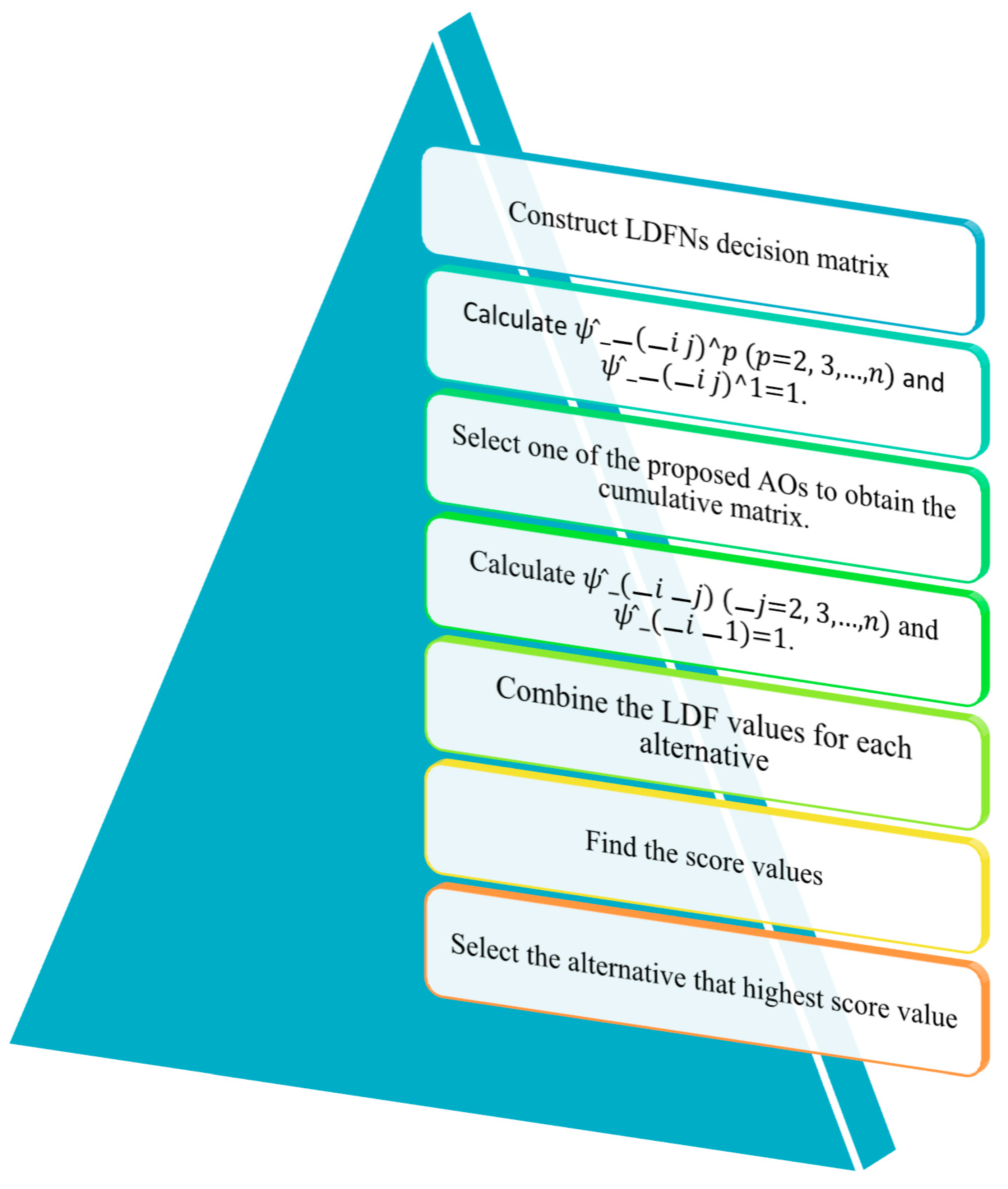
4. MCGDM Method with LDF Information

This section of the paper introduces the MCGDM approach using LDFHPWA and LDFHPWG AOs. We develop a Linear Diophantine fuzzy model to generate evaluation values. The computation stages for our proposed model are outlined below, assuming there are m ¯ alternatives Փ ~ 1 , Փ ~ 2 , Փ ~ 3 , , Փ ~ m ¯ , n ¯ criteria C ˘ 1 , C ˘ 2 , C ˘ 3 , , C ˘ n ¯ , and p experts { Đ ^ 1 ,   Đ ^ 2 ,   Đ ^ 3 , ,   Đ ^ p } . Prioritization among experts and criteria can be indicated by the ordering. Đ ^ 1 >   Đ ^ 2 >   Đ ^ 3 > > Đ ^ p   a n d   C ˘ 1 > C ˘ 2 > C ˘ 3 > > C ˘ n ¯ , where the criterion C ˘ i _ is preferred over the criterion C ˘ j _ , i _ < j _ . The DMs assessed the alternatives using various criteria, resulting in preference values in the form of LDFNs. Suppose that M = Ƣ i _ j _ p m ¯ × n ¯ = ɧ Ƣ i _ j _ p ,   Ӵ Ƣ i _ j _ p , E i _ j _ p ,   i _ j _ p m ¯ × n ¯ is the linear Diophantine fuzzy decision matrix, where ɧ Ƣ i _ j _ p represent the MD, Ӵ Ƣ i _ j _ p is the NMD, and E i _ j _ p , i _ j _ p are the RPs for which the alternative Փ ~ i _ satisfies the C ˘ i _ criteria provided by the DMs, where ɧ Ƣ i _ j _ p ,   Ӵ Ƣ i _ j _ p ,   E i _ j _ p ,   i _ j _ p 0 ,   1 such that 0 E ɧ Ƣ y j + Ӵ Ƣ   y j 1 with 0 E + 1 . The decision matrix M = Ƣ i _ j _ p m ¯ × n ¯ is a summary of the cumulative information of each decision maker. This model is highlighted in Figure 7. Here are the steps for computation as shown in Algorithm 1:
Algorithm 1
Step 1: Construct the LDF decision matrices M = Ƣ i _ j _ p m ¯ × n ¯ , where
i   =   1 ,   2,3 , , m ¯ ,   j   =   1 ,   2,3 , , n ¯ , and p =   1 ,   2 , , g can be illustrated as follows.
M = Ƣ i _ j _ p m ¯ × n ¯ =
  ɧ Ƣ 11 p ,   Ӵ Ƣ 11 p , E 11 p ,   11 p     ɧ Ƣ 12 p ,   Ӵ Ƣ 12 p , E 12 p ,   12 p       ɧ Ƣ 1 n ¯ p ,   Ӵ Ƣ 1 n ¯ p , E 1 n ¯ p ,   1 n ¯ p ɧ Ƣ 21 p ,   Ӵ Ƣ 21 p , E 21 p ,   21 p     ɧ Ƣ 22 p ,   Ӵ Ƣ 22 p , E 22 p ,   22 p         ɧ Ƣ 2 n ¯ p ,   Ӵ Ƣ 2 n ¯ p , E 2 n ¯ p ,   2 n ¯ p                                                                                                                             ɧ Ƣ m ¯ 1 p ,   Ӵ Ƣ m ¯ 1 p , E m ¯ 1 p ,   m ¯ 1 p   ɧ Ƣ m ¯ 2 p ,   Ӵ Ƣ m ¯ 2 p , E m ¯ 2 p ,   m ¯ 2 p     ɧ Ƣ m ¯ n ¯ p ,   Ӵ Ƣ m ¯ n ¯ p , E m ¯ n ¯ p ,   m ¯ n ¯ p
Step 2: Determine the value of ψ ^ i _ j _ p p = 1 ,   2 , , g as follows:
ψ ^ j _ p = l = 1 j _ 1 Տ ̿ Ƣ i _ j _ p such that ψ ^ 1 = 1 .
Step 3: Aggregate the LDF decision matrix M = Ƣ i _ j _ p m ¯ × n ¯ p =   1 ,   2 , , g into the combined LDF decision matrix M = Ƣ i _ j _ m ¯ × n ¯ by applying the LDFHPWA or LDFHPWG operator.
Step 4: Determine the value of ψ ^ i _ j _ = l = 1 j _ 1 Տ ̿ Ƣ i _ j _ , i = 1,2 , 3 , , m ¯ j = 1,2 , 3 , , n ¯ such that ψ ^ 1 = 1 .
Step 5: For each decision, aggregate all r ^ i =   j = 1,2 , 3 , , n ¯ . Use the LDFHPWA or LDFHPWG operator on Փ ~ i = i = 1,2 , 3 , , m ¯ .
Step 6: Rank every alternative Փ ~ i based on Փ ~ i i = 1,2 , 3 , , m ¯ using the score function.
Step 7: Select the alternative that has the greatest score.

5. Numerical Example

In this part, we present a numerical example demonstrating the applicability of our proposed technique. The problem is further solved using the processes outlined in the Algorithm. In many DM scenarios, criteria and decision makers (DMs) can have varying levels of priority. The prioritization of criteria significantly impacts the choice of operators in the DM process. In other words, using the same priority levels for both criteria and decision makers may lead to issues in certain situations. To address this issue, we opted to use prioritized AOs on LDFSs support systems, as they help mitigate these challenges. We considered three experts Đ ^ 1 , Đ ^ 2 , and Đ ^ 3 whoich provide information regarding cCybersecurity. Oon thise basis, we selected the best cybersecurity option to solve the MCGDM problem. Four cybersecurity options, namely, Փ ~ 1 : Encryption; Փ ~ 2 : Firewalls; Փ ~ 3 : Data Backup and Recovery; and Փ ~ 4 : Intrusion Detection and Prevention Systems, were assessed for selection following the initial assessment. Priority among DMs was Đ ^ 1 > Đ ^ 2 > Đ ^ 3 , suggesting that the DM Đ ^ 1 had greater prior than the other two, and the DM Đ ^ 2 had greater priority than Đ ^ 3 . The selection was completely neutral, which means it was devoid of any political or other influence. The selection experts evaluated the four Cybersecurity option based on the following five criteria:
  • C ˘ 1 : Security Effectiveness (SE)
  • C ˘ 2 : Cost-Effectiveness (CE)
  • C ˘ 3 : Network Segmentation (NS)
  • C ˘ 4 : Threat Intelligence (TI)
  • C ˘ 5 : Patch Management (PM)
C ˘ 1 was the most important criterion, followed by C ˘ 5 , which was the least important. As a result, the criteria weare prioritized as follows: C ˘ 1 > C ˘ 2 > C ˘ 3 > C ˘ 4 > C ˘ 5 . The DMs provided information in the form of LDFNs.

5.1. Explanation of Criteria

SE: The cybersecurity solution’s capability to accurately detect and prevent threats.
CE: The entire cost-benefit analysis of implementing a cybersecurity solution taking into account both the initial and continuing maintenance costs as well as the value it provides in terms of risk reduction.
NS: Partitioning the smart grid into distinct zones or segments helps to reduce the impact of security breaches and restricts attackers’ movement across various network areas.
TI: Leveraging advanced methods and tools, along with timely and accurate threat intelligence such as real-time threat detection, analysis, and sharing of compromise indicators, can significantly bolster proactive cybersecurity measures.
PM: The ability to effectively manage and implement software patches and updates to address security vulnerabilities and keep the system current with the latest protection measures.
Step 1: We constructed the LDF decision matrices M = Ƣ i _ j _ p 4 × 5 , where i   =   1 ,   2 , , 4 ,   j   =   1 ,   2 , , 5 , and p =   1 ,   2 ,   3 . It can be expressed as follows in Table 1, Table 2 and Table 3:
Step 2: We calculated the value of ψ ^ i _ j _ p p = 1 ,   2 ,   3 .
ψ ^ n _ m _ 1 = 1     1     1     1     1 1     1     1     1     1 1     1     1     1     1 1     1     1     1     1 ,   ψ ^ n _ m _ 2 = 0.5975     0.6025     0.5550     0.5575     0.5400 0.5275     0.4375     0.4950     0.5675     0.5725 0.5850     0.4800     0.5125     0.5325     0.6500 0.4775     0.4875     0.5375     0.5275     0.5425 ,
ψ ^ n _ m _ 3 = 0.3839     0.3419     0.3191     0.3554     0.2876 0.2796     0.1914     0.2364     0.3320     0.3363 0.3291     0.2304     0.2575   0.3208     0.3705 0.2507     0.2413     0.2943     0.2717     0.2631
Step 3: We aggregated the overall M = Ƣ i _ j _ p 4 × 5 to a single matrix M = Ƣ i _ j _ 4 × 5 by utilizing the LDFHPWA aggregation operator, where Ք ~ = 3 . Table 4 shows the calculated findings.
Step 4: We evaluated the values of ψ ~ i _ j _ i _ = 1,2 , , m ¯ , j _ = 1,2 , , n ¯
ψ ~ m ¯ n ¯ = 1     0.6547     0.3862     0.2187     0.1377 1     0.5244     0.2348     0.1152   0.0675 1     0.5750     0.2817     0.1460     0.0826 1     0.5146     0.2527     0.1381     0.0726
Step 5: We aggregated all r ^ i _ j _ = j = 1,2 , 3 , , n ¯ for each alternative Փ ~ i = i _ = 1,2 , 3 , , m ¯ and applied the LDFHPWA operator, where Ք ~ = 3 . Table 5 summarizes the relevant results.
Step 6: The score function was used to evaluate all the alternatives. Փ ~ i _ in accordance with r ^ i _ i _ = 1,2 , 3 , , m ¯ . Table 6, show the score values.
Step 7: We ranked the alternatives based on the score function Փ ~ 1 > Փ ~ 4 > Փ ~ 3 > Փ ~ 2 .

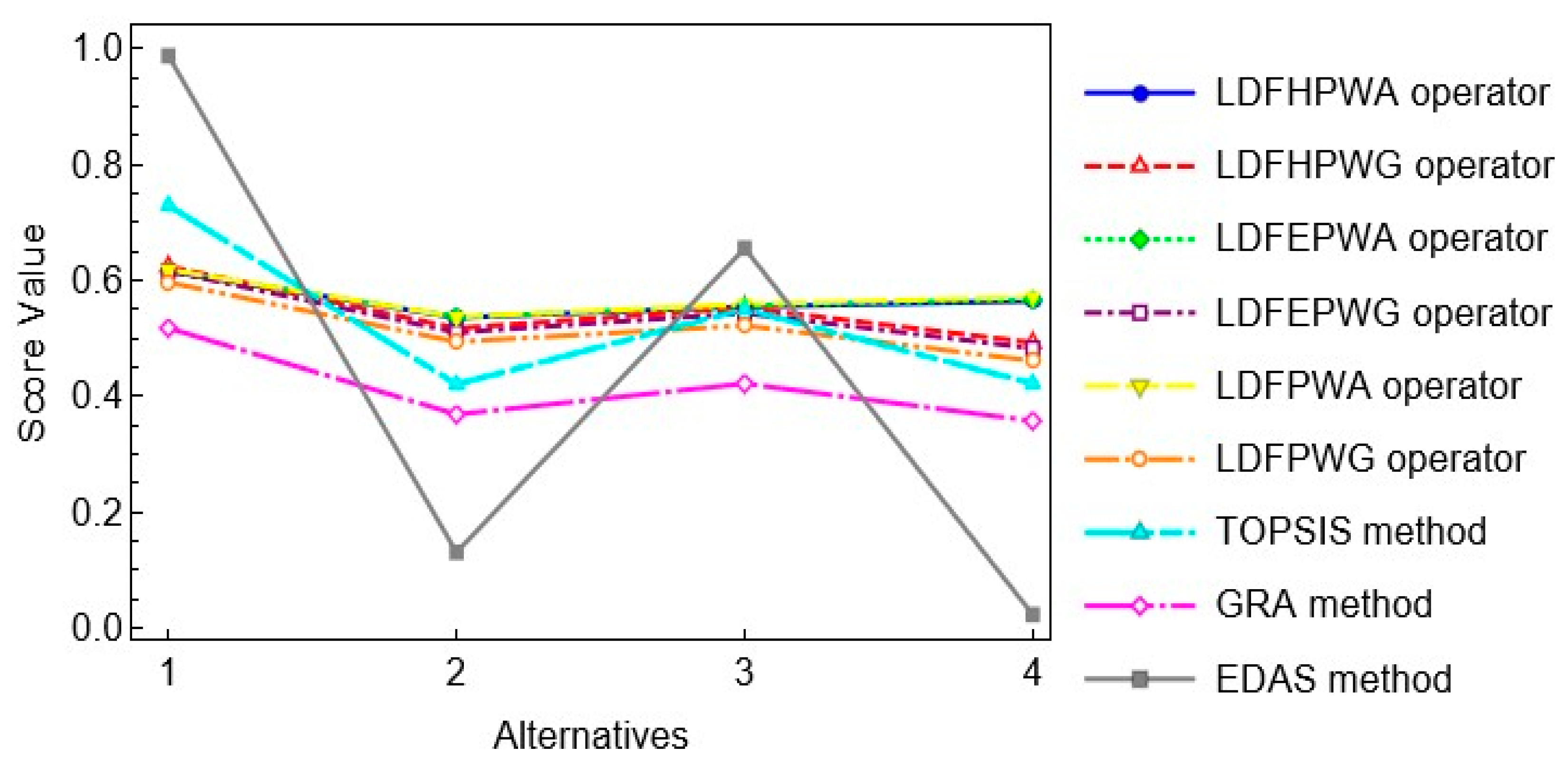
5.2. Comparison Analysis with Existing Methods

The suggested approaches for the MCGDM were validated and compared to current methods, as indicated in Table 7 and the corresponding graph is shown in Figure 8.
To compare our proposed operator with the LDFHPWG, LDFEPWA [51], LDFEPWG [51], LDFPWA [52], and LDFPWG [52] operators based on Equation (22), we considered the criteria weights of w = 0.25 ,   0.17 ,   0.13 ,   0.15 ,   0.30 T . We also compared with the TOPSIS method [53], GRA method [54], and EDAS method [55]. Table 7 demonstrates that the optimal alternative achieved by the proposed methods is identical to that of the LDFHPWG operator, LDFEPWA operator, LDFEPWG operator, LDFPWA operator, and LDFPWG operator as well as the TOPSIS method [53], GRA method [54], and EDAS method [55], demonstrating the viability of the proposed decision-making methods.

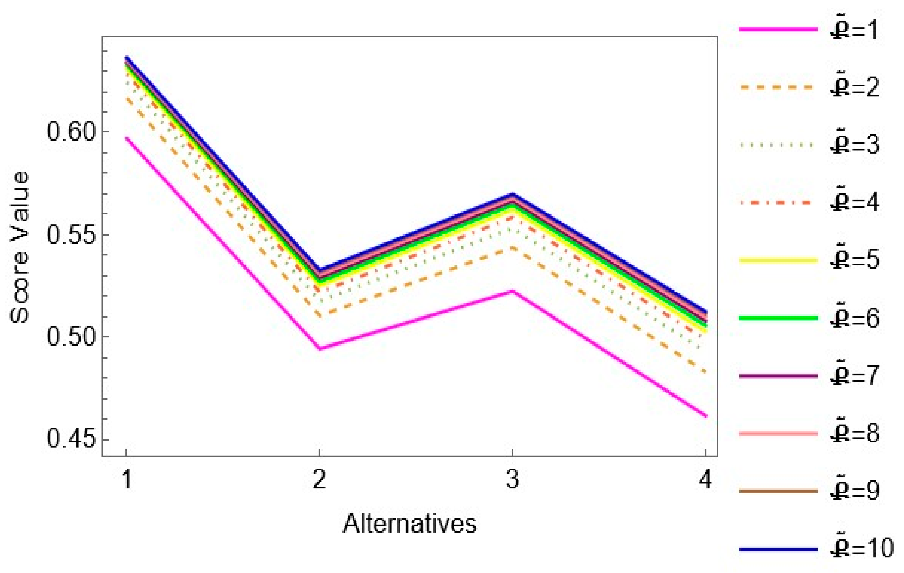
5.3. Sensitivity Analysis

To rank the given alternatives, we used various values for the operational parameter Ք ~ . For different parameter Ք ~ , we ranked the alternatives to show the benefits of the operational parameter Ք ~ on the MCGDM results. Table 8 and Table 9 indicate the effects of ranking alternative options Փ ~ 1 , Փ ~ 2 , Փ ~ 3 , Փ ~ 4 between 1 Ք ~ 10 according to the LDFHPWA and LDFHPWG operators, respectively. If the value of the parameter Ք ~ varied for the LDFHPWA operator, then the resultant appropriate alternatives are shown in Table 8. When 1 Ք ~ 10 , we observed that Փ ~ 1 > Փ ~ 4 > Փ ~ 3 > Փ ~ 2 , so the appropriate alternatives were ranked in the same order. The related graph is depicted in Figure 9. Table 9 clearly shows the resultant appropriate alternatives for the value of Ք ~ , which varied for the FFLDPWG operator. When, 1 Ք ~ 10 , we observed that Փ ~ 1 > Փ ~ 3 > Փ ~ 2 > Փ ~ 4 . The ranking of permissible alternatives for the FFLDPWG operator was significantly influenced by the working parameter values discussed in relation to MCGDM difficulties. Graphical view of 1 Ք ~ 10 , for alternatives is shown in Figure 10.

5.4. Advantages of the Proposed Method

a.
The most significant aspect of LDFSs is their capacity to express RP occurrences that require the allocation of MD and NMD. This feature makes LDFSs more dominating in expressing the needed information, overcoming the shortcomings of previous theories such as LDFSs and q-ROFSs.
b.
The LDFS model addresses imprecision and periodicity at the same time, expanding on prior models.
c.
Prioritized AOs capture prioritization phenomena among aggregated arguments, enhancing decision making in real-life scenarios. They were applied to LDFSs while maintaining their advantages.
d.
The suggested AOs are useful to aggregate fuzzy priorities and weights for evaluating alternatives in decision-making problems, such as project selection or resource allocation.
e.
The proposed method can be used to aggregate fuzzy opinions and priorities from multiple experts or stakeholders in group decision-making scenarios.
f.
The proposed method can be utilized to evaluate fuzzy quality metrics and prioritize weights for defect detection or quality improvement.
g.
The proposed approach is more versatile and convenient for handling common MCGDM issues.
h.
These applications leverage the ability of the implemented AOs to handle fuzzy information, prioritize weights, and aggregate data in a flexible and robust manner.

6. Conclusions

Selecting a cyber security system requires careful consideration of threat landscapes, vulnerability assessments, and organizational needs to ensure effective protection of assets, data, and infrastructure, warranting a comprehensive approach to mitigate risks and safeguard digital assets. Aggregation operators are essential in information fusion for real-world situations. The combination of RP with MD and NMD yields a unique concept for representing uncertainty in decision-making circumstances known as LDF information. First, we presented novel aggregation methods for modeling uncertainty based on linear Diophantine fuzzy data. We introduced prioritized weighted AOs for a set of LDFNs, including the LDFHPWA and LDFHPWG operators. Examining their significant characteristics in depth, we developed an MCGDM approach using prioritized AOs in an LDF context, focusing on prioritization relationships over criteria. The problem was mathematically described, followed by an algorithm and method flow chart. A numerical example of selecting cyber security system was shown to demonstrate the efficiency, superiority, and logic of the suggested technique. We also conducted a validation test to determine the effectiveness and validity of our suggested approach. We conducted a comparison study using the suggested operators with current literature operators to showcase their superiority. Based on the reasons presented above, it is argued that the current study provides more effective methods for managing complicated spherical fuzzy information in order to tackle real challenges.
Our future work will focus on tackling additional real-life situations with “Linear Diophantine fuzzy soft set” (LDFSS), “Linear Diophantine Hesitant fuzzy set” (LDHFS) and “Linear Diophantine fuzzy graphs” (LDF-graphs). Additionally, we will extend the suggested framework for the offshore wind turbine site selection as discussed by Karuppiah et al. [56] and intuitionistic fuzzy Sugeno–Weber decision framework for sustainable digital security assessment presented by Hussain et al. [57].

Author Contributions

Writing—original draft, M.Z.H., Writing—review & editing, N.Y. All authors have read and agreed to the published version of the manuscript.

Funding

This research received no external funding.

Data Availability Statement

Data are contained within the article.

Conflicts of Interest

The authors of this paper declare that they have no conflicts of interest.

References

  1. Bouramdane, A.A. Cyberattacks in smart grids: Challenges and solving the multi-criteria decision-making for cybersecurity options, including ones that incorporate artificial intelligence, using an analytical hierarchy process. J. Cybersecur. Priv. 2023, 3, 662–705. [Google Scholar] [CrossRef]
  2. Woo, P.S.; Kim, B.H. Methodology of cyber security assessment in the smart grid. J. Electr. Eng. Technol. 2017, 12, 495–501. [Google Scholar] [CrossRef]
  3. Ansari, M.; Asrari, A. Reaction to detected cyberattacks in smart distribution systems. In Proceedings of the 2020 IEEE Power & Energy Society Innovative Smart Grid Technologies Conference (ISGT), Washington, DC, USA, 17–20 February 2020; pp. 1–5. [Google Scholar]
  4. Alkuwari, A.N.; Al-Kuwari, S.; Qaraqe, M. Anomaly detection in smart grids: A survey from cybersecurity perspective. In Proceedings of the 2022 3rd International Conference on Smart Grid and Renewable Energy (SGRE), Doha, Qatar, 20–22 March 2022; pp. 1–7. [Google Scholar]
  5. Liu, Q.; Hagenmeyer, V.; Keller, H.B. A review of rule learning-based intrusion detection systems and their prospects in smart grids. IEEE Access 2021, 9, 57542–57564. [Google Scholar] [CrossRef]
  6. Alwageed, H.S. Detection of cyber attacks in smart grids using SVM-boosted machine learning models. Serv. Oriented Comput. Appl. 2022, 16, 313–326. [Google Scholar] [CrossRef]
  7. Zhai, F.; Yang, T.; Zhao, B.; Chen, H. Privacy-preserving outsourcing algorithms for multidimensional data encryption in smart grids. Sensors 2022, 22, 4365. [Google Scholar] [CrossRef] [PubMed]
  8. Miller, M.Z.; Griendling, K.; Mavris, D.N. Exploring human factors effects in the smart grid system of systems demand response. In Proceedings of the 2012 7th International Conference on System of Systems Engineering (SoSE), Genova, Italy, 16–19 July 2012; pp. 1–6. [Google Scholar]
  9. Fredman, D. A Human Side of the Smart Grid: Behavior-Based Energy Efficiency from Renters Using Real-Time Feedback and Competitive Performance-Based Incentives; The University of Vermont and State Agricultural College: Burlington, VT, USA, 2018. [Google Scholar]
  10. Montañez, R.; Golob, E.; Xu, S. Human cognition through the lens of social engineering cyberattacks. Front. Psychol. 2020, 11, 1755. [Google Scholar] [CrossRef]
  11. Ray, J.R. Training Programs to Increase Cybersecurity Awareness and Compliance in Non-Profits. 2014. Available online: https://scholarsbank.uoregon.edu/items/8a6c47a2-8e7d-4bc6-92df-719fb3ede12f (accessed on 2 December 2022).
  12. Loi, M.; Christen, M. Ethical frameworks for cybersecurity. In The Ethics of Cybersecurity; Springer: Berlin/Heidelberg, Germany, 2020; pp. 73–95. [Google Scholar]
  13. Rahman, M.A.; Manshaei, M.H.; Al-Shaer, E.; Shehab, M. Secure and private data aggregation for energy consumption scheduling in smart grids. IEEE Trans. Dependable Secur. Comput. 2015, 14, 221–234. [Google Scholar] [CrossRef]
  14. Albasrawi, M.N.; Jarus, N.; Joshi, K.A.; Sarvestani, S.S. Analysis of reliability and resilience for smart grids. In Proceedings of the 2014 IEEE 38th Annual Computer Software and Applications Conference, Vasteras, Sweden, 21–25 July 2014; pp. 529–534. [Google Scholar]
  15. Kanca, A.M.; Sağiroğlu, Ş. Sharing cyber threat intelligence and collaboration. In Proceedings of the 2021 International Conference on Information Security and Cryptology (ISCTURKEY), Ankara, Turkey, 2–3 December 2021; pp. 167–172. [Google Scholar]
  16. Majumder, M.; Majumder, M. Multi criteria decision making. In Impact of Urbanization on Water Shortage in Face of Climatic Aberrations; Springer: Berlin/Heidelberg, Germany, 2015; pp. 35–47. [Google Scholar]
  17. Triantaphyllou, E.; Triantaphyllou, E. Multi-Criteria Decision Making Methods; Springer: Berlin/Heidelberg, Germany, 2000; pp. 5–21. [Google Scholar]
  18. Zadeh, L.A. Fuzzy sets. Inf. Control 1965, 8, 338–353. [Google Scholar] [CrossRef]
  19. Atanassov, K.T. On Intuitionistic Fuzzy Sets Theory; Springer: Berlin/Heidelberg, Germany, 2012; Volume 283. [Google Scholar]
  20. Yager, R.R. Pythagorean fuzzy subsets. In Proceedings of the 2013 Joint IFSA World Congress and NAFIPS Annual Meeting (IFSA/NAFIPS), Edmonton, AB, Canada, 24–28 June 2013; pp. 57–61. [Google Scholar]
  21. Yager, R.R. Generalized orthopair fuzzy sets. IEEE Trans. Fuzzy Syst. 2016, 25, 1222–1230. [Google Scholar] [CrossRef]
  22. Khan, M.J.; Kumam, P.; Shutaywi, M.; Kumam, W. Improved Knowledge Measures for q-Rung Orthopair Fuzzy Sets. Int. J. Comput. Intell. Syst. 2021, 14, 1700–1713. [Google Scholar] [CrossRef]
  23. Khan, M.J.; Kumam, P.; Shutaywi, M. Knowledge measure for the q-rung orthopair fuzzy sets. Int. J. Intell. Syst. 2021, 36, 628–655. [Google Scholar] [CrossRef]
  24. Khan, M.J.; Ali, M.I.; Kumam, P.; Kumam, W.; Al-Kenani, A.N. q-Rung orthopair fuzzy modified dissimilarity measure based robust VIKOR method and its applications in mass vaccination campaigns in the context of COVID-19. IEEE Access 2021, 9, 93497–93515. [Google Scholar] [CrossRef]
  25. Riaz, M.; Hashmi, M.R. Linear Diophantine fuzzy set and its applications towards multi-attribute decision-making problems. J. Intell. Fuzzy Syst. 2019, 37, 5417–5439. [Google Scholar] [CrossRef]
  26. Iampan, A.; García, G.S.; Riaz, M.; Athar Farid, H.M.; Chinram, R. Linear Diophantine fuzzy Einstein aggregation operators for multi-criteria decision-making problems. J. Math. 2021, 1, 5548033. [Google Scholar] [CrossRef]
  27. Ayub, S.; Shabir, M.; Riaz, M.; Mahmood, W.; Bozanic, D.; Marinkovic, D. Linear diophantine fuzzy rough sets: A new rough set approach with decision making. Symmetry 2022, 14, 525. [Google Scholar] [CrossRef]
  28. Jeevitha, K.; Garg, H.; Vimala, J.; Aljuaid, H.; Abdel-Aty, A.H. Linear diophantine multi-fuzzy aggregation operators and its application in digital transformation. J. Intell. Fuzzy Syst. 2023, 45, 3097–3107. [Google Scholar] [CrossRef]
  29. Mohammad, M.M.S.; Abdullah, S.; Al-Shomrani, M.M. Some linear Diophantine fuzzy similarity measures and their application in decision making problem. IEEE Access 2022, 10, 29859–29877. [Google Scholar] [CrossRef]
  30. Xu, Z.; Yager, R.R. Some geometric aggregation operators based on intuitionistic fuzzy sets. Int. J. Gen. Syst. 2006, 35, 417–433. [Google Scholar] [CrossRef]
  31. Hamacher, H.; Trappl, R.; Klir, G.H.; Riccardi, L. In Progress in Cybernatics and Systems Research. Uber Logische Verknunpfungenn Unssharfer Aussagen Und Deren Zugenhorige Bewertungsfunktione 1978, 3, 276–288. [Google Scholar]
  32. Liu, P. Some Hamacher aggregation operators based on the interval-valued intuitionistic fuzzy numbers and their application to group decision making. IEEE Trans. Fuzzy Syst. 2013, 22, 83–97. [Google Scholar] [CrossRef]
  33. Tan, C.; Yi, W.; Chen, X. Hesitant fuzzy Hamacher aggregation operators for multicriteria decision making. Appl. Soft Comput. 2015, 26, 325–349. [Google Scholar] [CrossRef]
  34. Huang, J.Y. Intuitionistic fuzzy Hamacher aggregation operators and their application to multiple attribute decision making. J. Intell. Fuzzy Syst. 2014, 27, 505–513. [Google Scholar] [CrossRef]
  35. Wu, S.J.; Wei, G.W. Pythagorean fuzzy Hamacher aggregation operators and their application to multiple attribute decision making. Int. J. Knowl. Based Intell. Eng. Syst. 2017, 21, 189–201. [Google Scholar] [CrossRef]
  36. Darko, A.P.; Liang, D. Some q-rung orthopair fuzzy Hamacher aggregation operators and their application to multiple attribute group decision making with modified EDAS method. Eng. Appl. Artif. Intell. 2020, 87, 103259. [Google Scholar] [CrossRef]
  37. Shams, M.; Abdullah, S.; Khan, F.; Ali, R.; Muhammad, S. Fuzzy Decision Support Systems for Selection of NEA Detection Technologies Under Non-Linear Diophantine Fuzzy Hamacher Aggregation Information. IEEE Access 2024, 12, 32111–32139. [Google Scholar] [CrossRef]
  38. Zhang, S.; Li, X.; Meng, F. An approach to intuitionistic fuzzy multi-attribute group decision making based on hybrid Einstein aggregation operators. Int. J. Intell. Inf. Database Syst. 2016, 9, 315–343. [Google Scholar] [CrossRef]
  39. Hadi, A.; Khan, W.; Khan, A. A novel approach to MADM problems using Fermatean fuzzy Hamacher aggregation operators. Int. J. Intell. Syst. 2021, 36, 3464–3499. [Google Scholar] [CrossRef]
  40. Seikh, M.R.; Mandal, U. Intuitionistic fuzzy Dombi aggregation operators and their application to multiple attribute decision-making. Granul. Comput. 2021, 6, 473–488. [Google Scholar] [CrossRef]
  41. Akram, M.; Dudek, W.A.; Dar, J.M. Pythagorean Dombi fuzzy aggregation operators with application in multicriteria decision-making. Int. J. Intell. Syst. 2019, 34, 3000–3019. [Google Scholar] [CrossRef]
  42. Aydemir, S.B.; Yilmaz Gunduz, S. Fermatean fuzzy TOPSIS method with Dombi aggregation operators and its application in multi-criteria decision making. J. Intell. Fuzzy Syst. 2020, 39, 851–869. [Google Scholar] [CrossRef]
  43. Yager, R.R. Prioritized aggregation operators. Int. J. Approx. Reason. 2008, 48, 263–274. [Google Scholar] [CrossRef]
  44. Yu, D. Intuitionistic fuzzy prioritized operators and their application in multi-criteria group decision making. Technol. Econ. Dev. Econ. 2013, 19, 1–21. [Google Scholar] [CrossRef]
  45. Verma, R.; Sharma, B. Intuitionistic fuzzy Einstein prioritized weighted average operators and their application to multiple attribute group decision making. Appl. Math. Inf. Sci. 2015, 9, 3095. [Google Scholar]
  46. Arora, R.; Garg, H. Prioritized averaging/geometric aggregation operators under the intuitionistic fuzzy soft set environment. Sci. Iran 2018, 25, 466–482. [Google Scholar] [CrossRef]
  47. Khan, M.S.A.; Abdullah, S.; Ali, A.; Amin, F. Pythagorean fuzzy prioritized aggregation operators and their application to multi-attribute group decision making. Granul. Comput. 2019, 4, 249–263. [Google Scholar] [CrossRef]
  48. Gao, H. Pythagorean fuzzy Hamacher prioritized aggregation operators in multiple attribute decision making. J. Intell. Fuzzy Syst. 2018, 35, 2229–2245. [Google Scholar] [CrossRef]
  49. Jan, A.; Khan, A.; Khan, W.; Afridi, M. A novel approach to MADM problems using Fermatean fuzzy Hamacher prioritized aggregation operators. Soft Comput. 2021, 25, 13897–13910. [Google Scholar] [CrossRef]
  50. Akram, M.; Khan, A.; Alcantud, J.C.R.; Santos-García, G. A hybrid decision-making framework under complex spherical fuzzy prioritized weighted aggregation operators. Expert Syst. 2021, 38, e12712. [Google Scholar] [CrossRef]
  51. Riaz, M.; Farid, H.M.A.; Aslam, M.; Pamucar, D.; Bozanić, D. Novel approach for third-party reverse logistic provider selection process under linear Diophantine fuzzy prioritized aggregation operators. Symmetry 2021, 13, 1152. [Google Scholar] [CrossRef]
  52. Farid, H.M.A.; Riaz, M.; Khan, M.J.; Kumam, P.; Sitthithakerngkiet, K. Sustainable thermal power equipment supplier selection by Einstein prioritized linear Diophantine fuzzy aggregation operators. Aims Math. 2022, 7, 11201–11242. [Google Scholar] [CrossRef]
  53. Gül, S.; Aydoğdu, A. Novel distance and entropy definitions for linear Diophantine fuzzy sets and an extension of TOPSIS (LDF-TOPSIS). Expert Syst. 2023, 40, e13104. [Google Scholar] [CrossRef]
  54. Khan, M.S.A.; Jana, C.; Khan, M.T.; Mahmood, W.; Pal, M.; Mashwani, W.K. Extension of GRA method for multiattribute group decision making problem under linguistic Pythagorean fuzzy setting with incomplete weight information. Int. J. Intell. Syst. 2022, 37, 9726–9749. [Google Scholar] [CrossRef]
  55. Qiyas, M.; Khan, N.; Naeem, M.; Okyere, S. Decision-Making Based on Spherical Linear Diophantine Fuzzy Rough Aggregation Operators and EDAS Method. J. Math. 2023, 2023, 5839410. [Google Scholar] [CrossRef]
  56. Karuppiah, K.; Sankaranarayanan, B.; Ali, S.M.; Marimuthu, U. Integrated approach for offshore wind turbine site selection: Implications for sustainability in power supply chain. Energies 2024, 17, 3419. [Google Scholar] [CrossRef]
  57. Hussain, A.; Ullah, K.; Pamucar, D.; Simic, V. Intuitionistic fuzzy Sugeno-Weber decision framework for sustainable digital security assessment. Eng. Appl. Artif. Intell. 2024, 137, 109085. [Google Scholar] [CrossRef]
Disclaimer/Publisher’s Note: The statements, opinions and data contained in all publications are solely those of the individual au-thor(s) and contributor(s) and not of MDPI and/or the editor(s). MDPI and/or the editor(s) disclaim responsibility for any injury to people or property resulting from any ideas, methods, instructions or products referred to in the content.
Figure 1. A visual representation depicting the different types of cyberattacks.
Symmetry 17 00070 g001
Figure 2. Graphical comparison of space in IFS, PFS, FFS, and q-ROFFS.
Symmetry 17 00070 g002
Figure 3. LDF with E , = 0.6,0.3 .
Symmetry 17 00070 g003
Figure 4. LDF with E , = 0.9,0.01 .
Symmetry 17 00070 g004
Figure 5. LDF with E , = 0.8,0.09 .
Symmetry 17 00070 g005
Figure 6. Different parameters of LDF space.
Symmetry 17 00070 g006
Figure 7. Flow chart to determine best alternative.
Symmetry 17 00070 g007
Figure 8. Graphical representation of comparisons.
Symmetry 17 00070 g008
Figure 9. Visual depiction of the LDFHPWA operator with various parameters.
Symmetry 17 00070 g009
Figure 10. Visual depiction of the LDFHPWG operator with various parameters.
Symmetry 17 00070 g010
Table 1. LDF decision matrix Đ ^ 1 .
C ˘ 1 C ˘ 2 C ˘ 3 C ˘ 4 C ˘ 5
Փ ~ 1 0.75 ,   0.60 , 0.61 ,   0.37 1.00 ,   0.80 , 0.60 ,   0.39 1.00 ,   1.00 , 0.59 ,   0.37 0.90 ,   0.73 , 0.49 ,   0.43 0.88 ,   0.85 , 0.56 ,   0.43
Փ ~ 2 1.00 ,   1.00 , 0.49 ,   0.38 0.63 ,   1.00 , 0.54 ,   0.42 0.76 ,   1.00 , 0.50 ,   0.28 0.94 ,   0.73 , 0.50 ,   0.44 0.90 ,   0.82 , 0.59 ,   0.38
Փ ~ 3 1.00 ,   1.00 , 0.59 ,   0.25 1.00 ,   0.89 , 0.39 ,   0.58 0.96 ,   1.00 , 0.30 ,   0.21 0.80 ,   0.78 , 0.55 ,   0.44 0.75 ,   0.65 , 0.73 ,   0.23
Փ ~ 4 0.56 ,   0.65 , 0.50 ,   0.50 0.90 ,   1.00 , 0.20 ,   0.15 0.97 ,   0.89 , 0.43 ,   0.36 1.00 ,   1.00 , 0.50 ,   0.39 1.00 ,   0.89 , 0.52 ,   0.46
Table 2. LDF decision matrix Đ ^ 2 .
C ˘ 1 C ˘ 2 C ˘ 3 C ˘ 4 C ˘ 5
Փ ~ 1 0.70 ,   0.50 , 0.67 ,   0.30 0.91 ,   0.69 , 0.51 ,   0.46 1.00 ,   0.99 , 0.56 ,   0.27 0.95 ,   0.70 , 0.60 ,   0.30 0.80 ,   0.79 , 0.55 ,   0.43
Փ ~ 2 1.00 ,   0.97 , 0.48 ,   0.39 0.61 ,   1.00 , 0.56 ,   0.42 0.79 ,   1.00 , 0.40 ,   0.28 0.96 ,   0.73 , 0.54 ,   0.43 0.90 ,   0.82 , 0.58 ,   0.31
Փ ~ 3 1.00 ,   0.99 , 0.59 ,   0.35 1.00 ,   0.89 , 0.39 ,   0.58 1.00 ,   1.00 , 0.30 ,   0.29 0.75 ,   0.71 , 0.66 ,   0.29 0.85 ,   0.65 , 0.53 ,   0.45
Փ ~ 4 0.80 ,   0.77 , 0.53 ,   0.46 0.90 ,   1.00 , 0.37 ,   0.29 0.90 ,   0.81 , 0.41 ,   0.31 1.00 ,   1.00 , 0.45 ,   0.39 0.90 ,   0.89 , 0.42 ,   0.49
Table 3. LDF decision matrix Đ ^ 3 .
C ˘ 1 C ˘ 2 C ˘ 3 C ˘ 4 C ˘ 5
Փ ~ 1 1.00 ,   0.90 , 0.50 ,   0.47 1.00 ,   0.99 , 0.60 ,   0.40 0.98 ,   0.93 , 0.62 ,   0.36 1.00 ,   0.72 , 0.75 ,   0.20 1.00 ,   0.87 , 0.55 ,   0.42
Փ ~ 2 0.99 ,   1.00 , 0.45 ,   0.44 0.88 ,   1.00 , 0.54 ,   0.43 0.85 ,   1.00 , 0.50 ,   0.39 0.90 ,   0.63 , 0.60 ,   0.33 0.88 ,   0.77 , 0.49 ,   0.40
Փ ~ 3 1.00 ,   1.00 , 0.53 ,   0.28 0.99 ,   0.89 , 0.50 ,   0.41 1.00 ,   1.00 , 0.44 ,   0.34 0.89 ,   0.80 , 0.63 ,   0.35 0.71 ,   0.63 , 0.69 ,   0.29
Փ ~ 4 0.86 ,   0.75 , 0.62 ,   0.34 0.90 ,   1.00 , 0.29 ,   0.26 0.91 ,   0.87 , 0.59 ,   0.40 0.95 ,   1.00 , 0.56 ,   0.41 1.00 ,   1.00 , 0.52 ,   0.44
Table 4. Aggregated values by using LDFHPWA operator.
Ք ~ = 3 C ˘ 1 C ˘ 2 C ˘ 3 C ˘ 4 C ˘ 5
Փ ~ 1 1.00 ,   0.62 , 0.61 ,   0.36 1.00 ,   0.80 , 0.57 ,   0.41 1.00 ,   0.98 , 0.59 ,   0.34 1.00 ,   0.72 , 0.58 ,   0.34 1.00 ,   0.84 , 0.56 ,   0.43
Փ ~ 2 1.00 ,   0.99 , 0.48 ,   0.39 0.67 ,   1.00 , 0.54 ,   0.42 0.78 ,   1.00 , 0.47 ,   0.29 0.94 ,   0.71 , 0.53 ,   0.42 0.90 ,   0.81 , 0.57 ,   0.36
Փ ~ 3 1.00 ,   1.00 , 0.58 ,   0.28 1.00 ,   0.89 , 0.40 ,   0.56 1.00 ,   1.00 , 0.32 ,   0.25 0.81 ,   0.76 , 0.60 ,   0.38 0.78 ,   0.65 , 0.66 ,   0.30
Փ ~ 4 0.69 ,   0.70 , 0.53 ,   0.46 0.90 ,   1.00 , 0.26 ,   0.20 0.95 ,   0.86 , 0.45 ,   0.35 1.00 ,   1.00 , 0.50 ,   0.39 1.00 ,   0.91 , 0.49 ,   0.46
Table 5. Apply LDFHPWA operator to aggregate alternatives.
Ք ~ = 3 Aggregated Alternatives
Փ ~ 1 1.0000 ,   0.7529 , 0.5902 ,   0.3740
Փ ~ 2 1.0000 ,   0.9734 , 0.5039 ,   0.3869
Փ ~ 3 1.0000 ,   0.9398 , 0.5070 ,   0.3486
Փ ~ 4 1.0000 ,   0.8293 , 0.4482 ,   0.3602
Table 6. Overall, the score of the LDFHPWA operator.
Ք ~ = 3 Score Value
Տ ̿ Փ ~ 1 0.6158
Տ ̿ Փ ~ 2 0.5359
Տ ̿ Փ ~ 3 0.5547
Տ ̿ Փ ~ 4 0.5647
Table 7. Comparative analysis and ranking of alternatives.
Տ ̿ Փ ~ 1 Տ ̿ Փ ~ 2 Տ ̿ Փ ~ 3 Տ ̿ Փ ~ 4 Ranking
LDFHPWA operator 0.61580.53590.55470.5647 Փ ~ 1 > Փ ~ 4 > Փ ~ 3 > Փ ~ 2
Percentage 0.0061580.0053590.0055470.005647 Փ ~ 1 > Փ ~ 4 > Փ ~ 3 > Փ ~ 2
LDFHPWG operator 0.62440.51760.55310.4928 Փ ~ 1 > Փ ~ 3 > Փ ~ 2 > Փ ~ 4
Percentage 0.0062440.0051760.0055310.004928 Փ ~ 1 > Փ ~ 3 > Փ ~ 2 > Փ ~ 4
LDFEPWA operator [52]0.61710.53650.55640.5673 Փ ~ 1 > Փ ~ 4 > Փ ~ 3 > Փ ~ 2
Percentage 0.0061710.0053650.0055640.005673 Փ ~ 1 > Փ ~ 4 > Փ ~ 3 > Փ ~ 2
LDFEPWG operator [52]0.61670.51040.54380.4829 Փ ~ 1 > Փ ~ 3 > Փ ~ 2 > Փ ~ 4
Percentage 0.0061670.0051040.0054380.004829 Փ ~ 1 > Փ ~ 3 > Փ ~ 2 > Փ ~ 4
LDFPWA operator [51]0.61880.53740.55930.5714 Փ ~ 1 > Փ ~ 4 > Փ ~ 3 > Փ ~ 2
Percentage 0.0061880.0053740.0055930.005714 Փ ~ 1 > Փ ~ 4 > Փ ~ 3 > Փ ~ 2
LDFPWG operator [51]0.59690.49420.52240.4614 Փ ~ 1 > Փ ~ 3 > Փ ~ 2 > Փ ~ 4
Percentage 0.0059690.0049420.0052240.004614 Փ ~ 1 > Փ ~ 3 > Փ ~ 2 > Փ ~ 4
TOPSIS method [53]0.72970.42080.55050.4220 Փ ~ 1 > Փ ~ 3 > Փ ~ 4 > Փ ~ 2
Percentage 0.0072970.0042080.0055050.00422 Փ ~ 1 > Փ ~ 3 > Փ ~ 4 > Փ ~ 2
GRA method [54]0.51800.36900.42200.3575 Փ ~ 1 > Փ ~ 3 > Փ ~ 2 > Փ ~ 4
Percentage 0.005180.003690.004220.003575 Փ ~ 1 > Փ ~ 3 > Փ ~ 2 > Փ ~ 4
EDAS method [55]0.98800.13070.65580.0230 Փ ~ 1 > Փ ~ 3 > Փ ~ 2 > Փ ~ 4
Percentage 0.009880.0013070.0065580.00023 Փ ~ 1 > Փ ~ 3 > Փ ~ 2 > Փ ~ 4
Table 8. Decision results for LDFHPWA operator using different parameters.
Ք ~ Տ ̿ Փ ~ 1 Տ ̿ Փ ~ 2 Տ ̿ Փ ~ 3 Տ ̿ Փ ~ 4 Ranking
10.61880.53740.55930.5714 Փ ~ 1 > Փ ~ 4 > Փ ~ 3 > Փ ~ 2
20.61710.53650.55640.5673 Փ ~ 1 > Փ ~ 4 > Փ ~ 3 > Փ ~ 2
30.61580.53590.55470.5647 Փ ~ 1 > Փ ~ 4 > Փ ~ 3 > Փ ~ 2
40.61480.53540.55340.5627 Փ ~ 1 > Փ ~ 4 > Փ ~ 3 > Փ ~ 2
50.61400.53510.55250.5612 Փ ~ 1 > Փ ~ 4 > Փ ~ 3 > Փ ~ 2
60.61340.53480.55180.5599 Փ ~ 1 > Փ ~ 4 > Փ ~ 3 > Փ ~ 2
70.61280.53450.55120.5588 Փ ~ 1 > Փ ~ 4 > Փ ~ 3 > Փ ~ 2
80.61230.53430.55060.5578 Փ ~ 1 > Փ ~ 4 > Փ ~ 3 > Փ ~ 2
90.61180.53410.55020.5570 Փ ~ 1 > Փ ~ 4 > Փ ~ 3 > Փ ~ 2
100.61140.53400.54980.5562 Փ ~ 1 > Փ ~ 4 > Փ ~ 3 > Փ ~ 2
Table 9. Decision results for LDFHPWG operator using different parameters.
Ք ~ Տ ̿ Փ ~ 1 Տ ̿ Փ ~ 2 Տ ̿ Փ ~ 3 Տ ̿ Փ ~ 4 Ranking
10.59690.49420.52240.4614 Փ ~ 1 > Փ ~ 3 > Փ ~ 2 > Փ ~ 4
20.61670.51040.54380.4829 Փ ~ 1 > Փ ~ 3 > Փ ~ 2 > Փ ~ 4
30.62440.51760.55310.4928 Փ ~ 1 > Փ ~ 3 > Փ ~ 2 > Փ ~ 4
40.62850.52190.55850.4987 Փ ~ 1 > Փ ~ 3 > Փ ~ 2 > Փ ~ 4
50.63100.52490.56200.5026 Փ ~ 1 > Փ ~ 3 > Փ ~ 2 > Փ ~ 4
60.63280.52710.56450.5056 Փ ~ 1 > Փ ~ 3 > Փ ~ 2 > Փ ~ 4
70.63400.52890.56630.5078 Փ ~ 1 > Փ ~ 3 > Փ ~ 2 > Փ ~ 4
80.63500.53040.56780.5096 Փ ~ 1 > Փ ~ 3 > Փ ~ 2 > Փ ~ 4
90.63580.53160.56900.5111 Փ ~ 1 > Փ ~ 3 > Փ ~ 2 > Փ ~ 4
100.63640.53270.56990.5123 Փ ~ 1 > Փ ~ 3 > Փ ~ 2 > Փ ~ 4
Disclaimer/Publisher’s Note: The statements, opinions and data contained in all publications are solely those of the individual author(s) and contributor(s) and not of MDPI and/or the editor(s). MDPI and/or the editor(s) disclaim responsibility for any injury to people or property resulting from any ideas, methods, instructions or products referred to in the content.

