1. Introduction
Inthe contemporary digital age, image processing technology is assuming an increasingly pivotal role in a multitude of fields. Image alignment is a crucial issue in the field of computer vision, with applications in image stitching [
1], object recognition [
2], 3D reconstruction [
3], and other areas. Its use in these contexts has the potential to enhance image quality and accuracy, which is of great significance.
Conventional alignment techniques for image stitching are typically founded upon pixel alignment discrepancies and feature point-based image warping. These techniques generally align the images by evaluating the homography of the two images, which is an invertible mapping of a plane in two viewpoints. Pixel alignment error-based methods optimize the homography parameter between two images by iterating [
4], but this method generally yields superior results only when the overlap is high. Conventional feature-point-based image alignment methods typically employ disparate feature extractors [
5,
6,
7] and robustness estimation methods [
8,
9] to identify the feature points following exact matching. These methods then utilize distinct alignment strategies to align the images. Alignment strategies such as APAP [
10] employ a grid-based approach to align the image as much as possible. SVA [
11] introduces a smoothly varying affine stitching field while retaining the good extrapolation and occlusion processing properties of the parametric transforms. ELA [
12] is a robust image stitching method based on the TPS [
13] transform for addressing the parallax-tolerance issue in image stitching. TFA [
14] employs the technique of triangular facet approximation, which divides the image into small triangular facets and performs locally adaptive image alignment for each triangular region. SPHP [
15] employs the semi-projective transform, which lies between affine and projective transforms, to transform the image, thereby preserving its underlying geometry to a certain extent. GSP [
16] enhances image stitching by introducing global similarity a priori information, which results in a more natural and coherent stitching outcome. AANAP [
17] proposes a novel image stitching method that combines multiple techniques to render the panorama more natural. DHW [
18] utilizes two homographies to better align the image. However, feature point-based image alignment methods are subject to certain limitations when applied to low-texture and low-light images. For instance, uneven distribution of feature points can occur when the light is not uniform, which can result in distorted alignment results in regions with fewer features. Additionally, insufficient numbers of matching feature points can be encountered in low-overlap images, which can lead to failure to align due to insufficient feature points.
In comparison to traditional methods, deep learning image stitching methods [
19,
20,
21,
22] predict four point displacements of an image and solve for a global homography, a homography that only describes the mapping relationship of points on the same plane in two viewpoints. Consequently, this has limitations when dealing with parallax. Ref. [
23] proposed a method of meshing the image and predicting four point displacements for each mesh in order to solve for a multigrid homography. This enables multigrid warping in deep learning, but the problem of not being able to determine the pixel-point mapping relationship occurs when going beyond the mesh space. Consequently, obtaining the final stitched image is difficult. Furthermore, due to the prediction of displacements of mesh points, it is not possible to apply traditional image alignment algorithms to the field of homography.
To address these challenges, this study proposes a predictive feature point method based on deep learning. This method enhances the robustness of deep feature extraction by exploring the matching relationship between deep feature maps. The combination of the traditional APAP (As-projective-as-possible image stitching with moving DLT) multigrid image alignment algorithm with the field of deep learning enables the application of the traditional image alignment algorithm to deep learning, thereby improving the accuracy and robustness of image alignment. In order to obtain a complete stitched image, we introduce a mesh shape-preserving loss and train the model by distorting the target image. After the model is trained, we obtain a complete distorted image by chunking the reference image and reverse distorting it to obtain a complete stitched image by combining it with the target image. Our method employs multi-grid homography estimation to address challenging scenarios, thereby enhancing alignment accuracy in comparison to existing deep learning methods [
22] that predict a global homography.
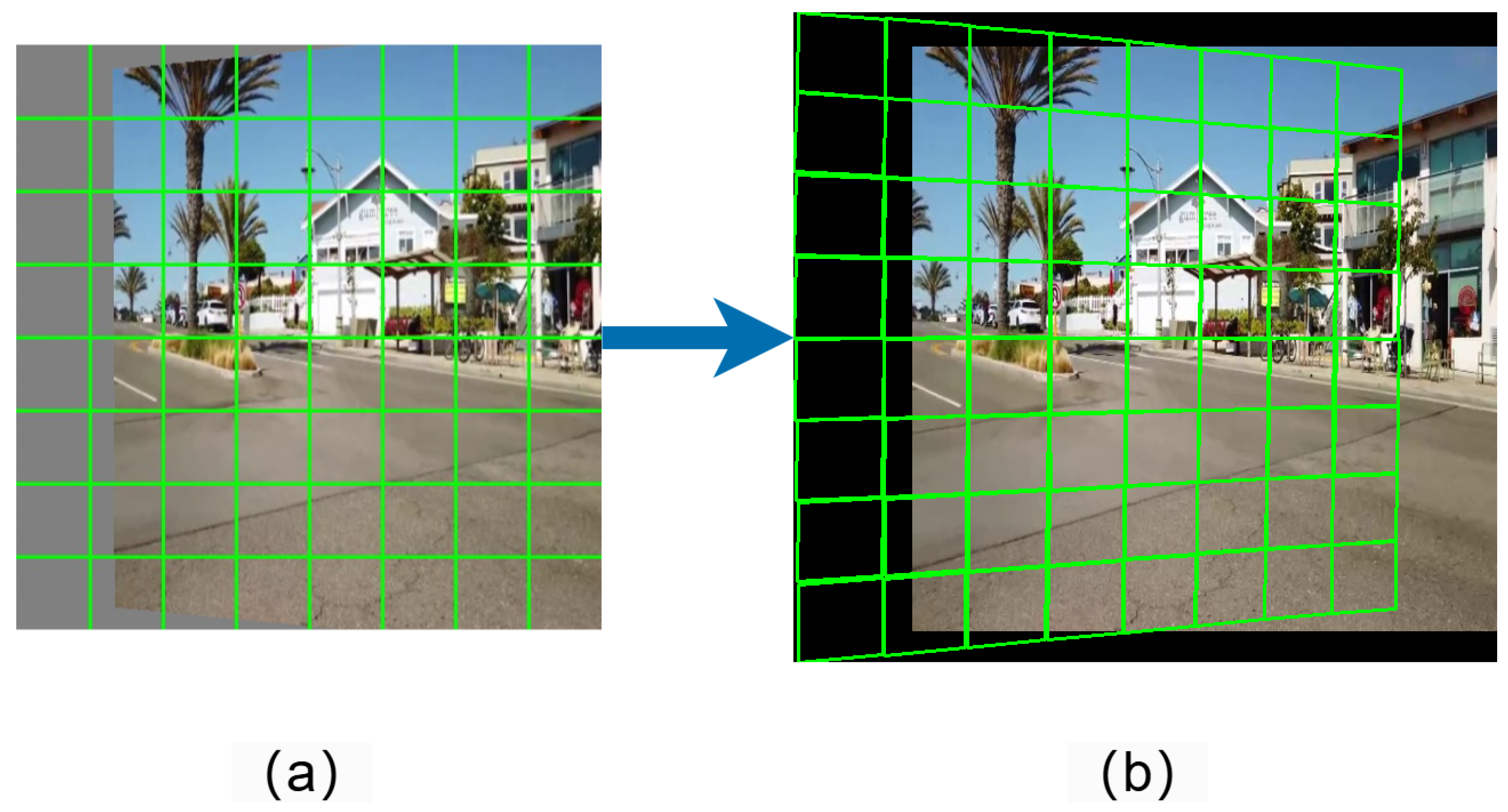
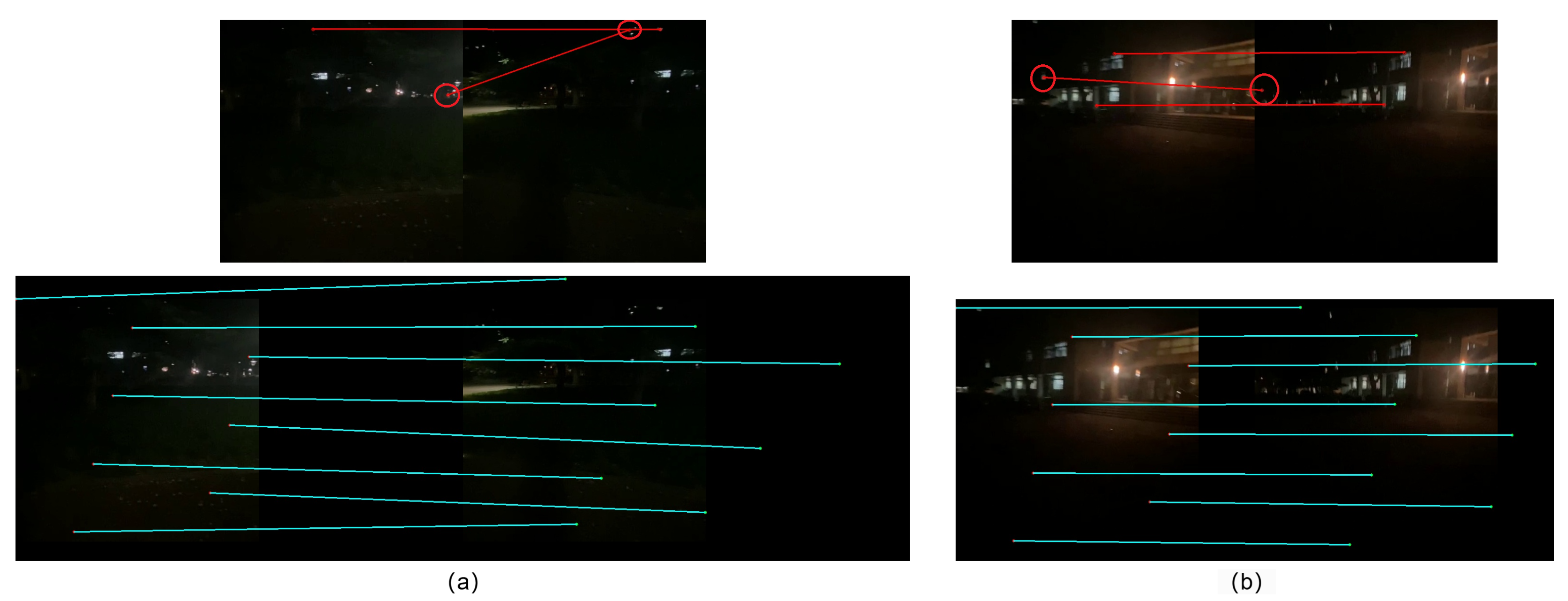
Specifically, our method employs singular value decomposition (SVD) to solve the homography of each grid. This is achieved by first obtaining a weighted map of all feature points in each grid. This is conducted by assuming a uniform distribution of feature points, predicting the displacements of the feature points, and simultaneously calculating the weights of each feature point within each grid. Subsequently, the accurate image alignment is achieved by warping the target image in the grid space. The proposed framework can be readily trained in an unsupervised manner using pixel-level content loss. Additionally, we introduce a shape-preserving loss to constrain the mesh inverse warping, thereby preventing the stitched images from appearing cracked (see
Figure 1b). Once training is complete, the reference image is divided into grid form. The invertibility of the homography matrix is then employed to inverse warp the corresponding image blocks, resulting in a warped map of each image block in the target image space. Finally, all the warped image blocks are synthesized into a complete warped map, which is then spliced with the target image.
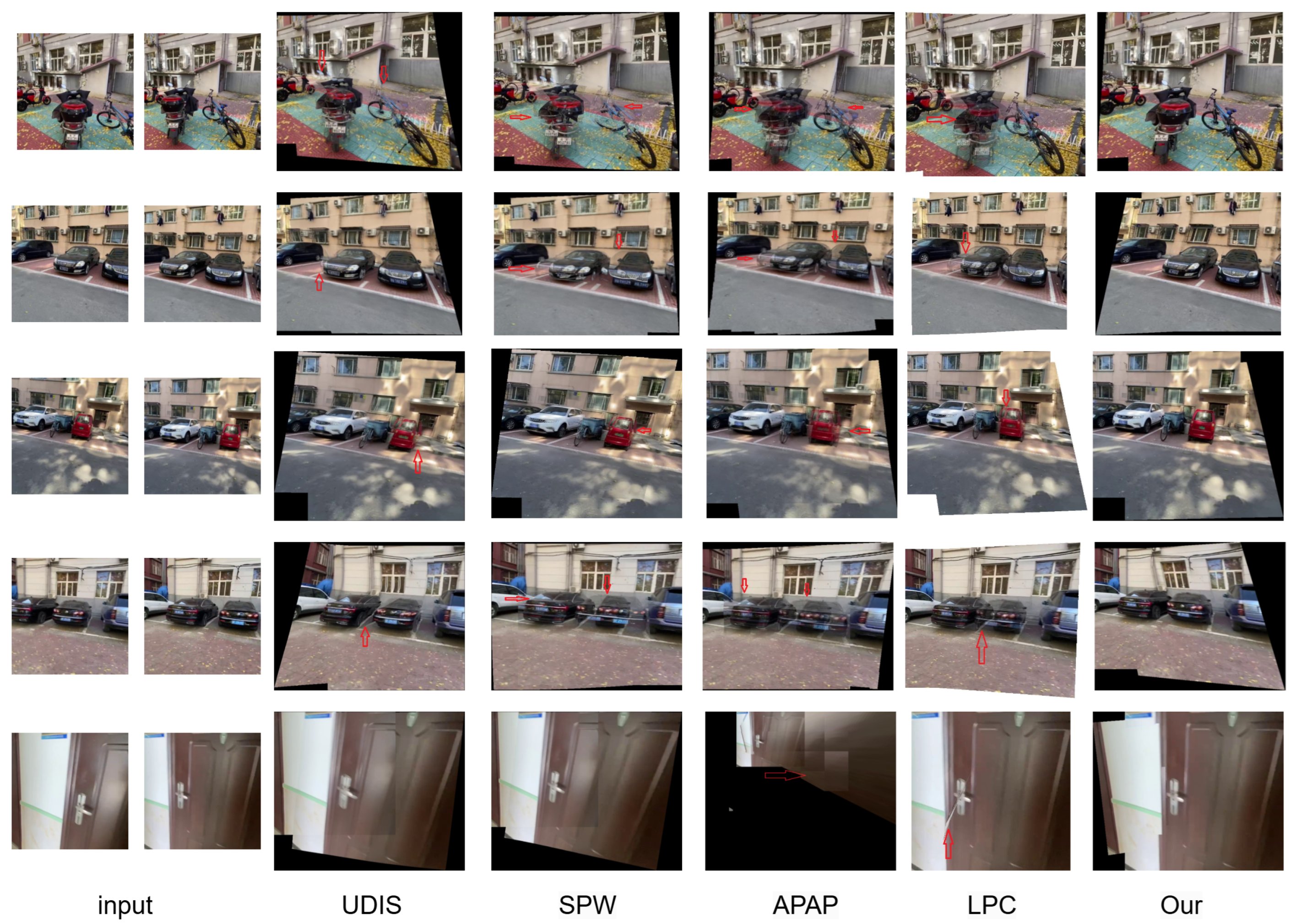
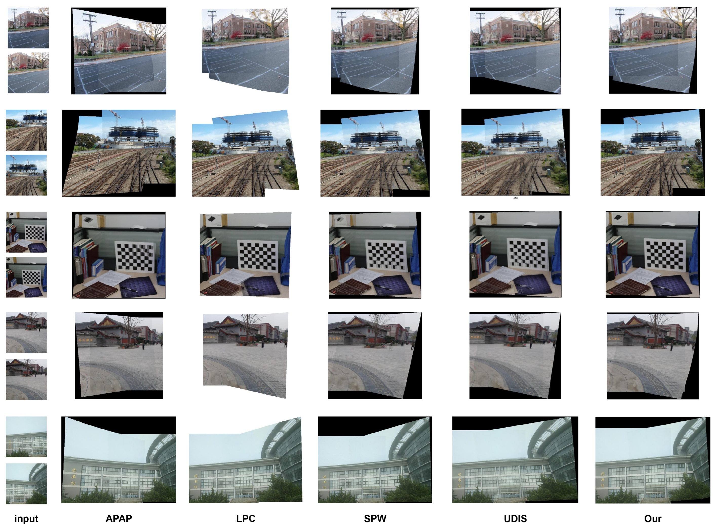
In the course of our experiments, we assess the efficacy of our approach in the domains of homography estimation, image alignment, and feature point prediction. The experimental results in real scenarios demonstrate the superiority of the method. The principal contributions of this paper are as follows:
1. A deep learning network for predicting feature points is proposed. This network achieves more robust deep feature extraction and ensures that the network outputs the desired number of feature points in any case by custom setting the number of feature points.
2. The APAP multigrid deformation parameterization was implemented for unsupervised multigrid graph alignment.
3. Image chunking inverse warping and mesh shape-preserving loss are proposed. This is achieved by first chunking the reference image, inverting the image chunks using the invertibility of the singular response matrix, and then using the mesh shape-preserving loss to constrain the distances between image chunks in order to obtain a complete spliced image.
3. Methodological Process
The method comprises two stages: deep multigrid warping and chunked inverse transformation. In the initial stage, as illustrated in
Figure 2, our method accepts the reference image
and the target image
as inputs, generates the displacements of the feature points, and then computes the weight matrix
W and multiplies it with the feature point mapping relation matrix
A. The distortion matrix of the multigrid is obtained by singular value decomposition of the matrix
. The second stage is depicted in
Figure 3. It involves the segmentation of the reference image, the application of an inverse transformation superposition to all image segments, the generation of the reference image in the target image view, and the weighted average fusion of the overlapping regions to obtain the final panorama.
3.1. Multi-Mesh Warping Parameterization
The homography transform is a common method for image alignment. It is an invertible mapping from one picture to another with eight degrees of freedom. Every two degrees of freedom are used for translation, rotation, scaling, and straight lines at infinity. However, the homography transform is only capable of aligning a single plane and is, therefore, inadequate for aligning the real picture. The APAP algorithm, a traditional method, is more effective for this problem. However, the algorithm is based on a traditional feature point extraction method, which may result in difficulties aligning the image when the distribution of image feature points is not uniform or there are not enough feature points. While deep learning methods can effectively address this issue, the current deep learning frameworks are primarily based on the displacement prediction of grid points, which limits their ability to utilize the APAP alignment algorithm effectively. To address this issue, a parameterization of APAP warping is implemented, assuming that the feature points are uniformly distributed on the image in the shape of grid points. Deep learning is employed to predict the displacement of each feature point, calculate the weight of each feature point in each grid, and identify the homography of each grid through singular value decomposition.
The APAP alignment algorithm computes the local homography of each grid by matching two sets of feature points,
of the reference image and
of the distorted image. The assumption is that
is uniformly distributed in the form of a grid on the reference image, and that
is obtained by the deep learning network by predicting the displacements and then summing them up with
. The
i-th pair of feature points is defined as
. Let
be the set of grid centers and
the center of the
k-th grid. Based on the distance between the reference image feature points and ck, the weight
of each feature point in the local distortion of the
k-th grid can be calculated.
The scale parameter, denoted by , is used to determine the scale of the feature points, while the parameter is employed to restrict the minimum weight of the feature points. When equals one, the distortion becomes a global projection distortion.
Let the projection matrix be
.
The value of
represents the
i-th row of
. The Equation (3) can be derived by utilising a pair of feature points.
By employing all available feature points, the following equation can be derived.
The minimal effective right singular vector, designated as
, can be derived through the singular value decomposition of the matrix comprising all the feature points.
The value of
is obtained by vertically stacking all values of
, while the value of
represents the lowest effective right singular vector. The local deformation matrix,
, for the
k-th mesh is computed as follows:
where
. The minimum singular right vector
is obtained by performing a singular value decomposition of
.
The objective is to determine the homography matrix
H for all meshes.
where
.
In our research on the multigrid twisted transform parameterization, we define feature points to be uniformly distributed over the image as grid points and then predict the displacement of these points. The weights of the feature points within each grid are calculated, and singular value decomposition (SVD) is employed to identify the homography of each grid.
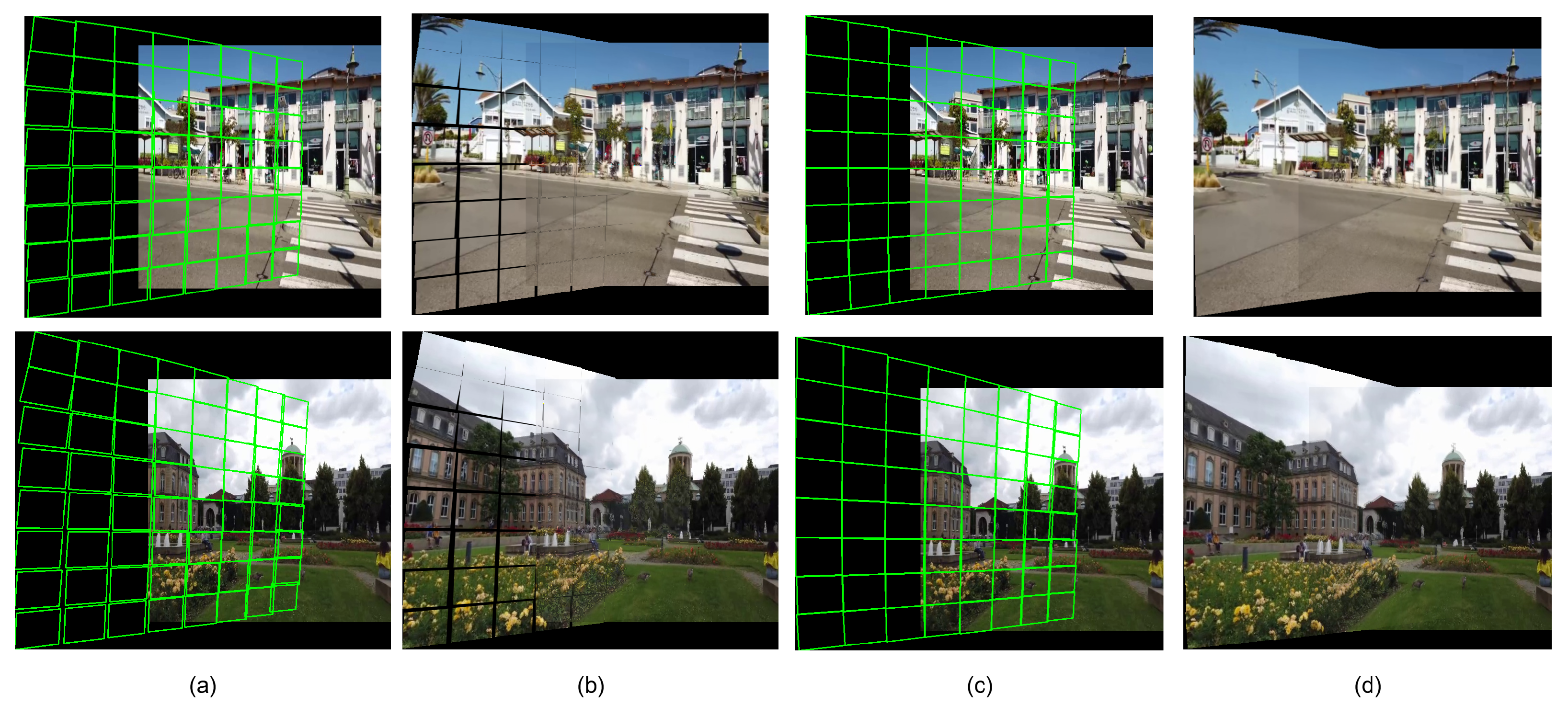
3.2. Network Framework
Figure 2 provides a concise overview of the multigrid deep homography network. Images
and
are processed to extract semantic features using a ResNet50 [
34] model that maps the image to
resolution feature blocks. This is subsequently mapped into a two-channel
feature stream using the Contextual Correlation Layer [
23], and the input feature stream is then predicted using a regression network with
displacement parameters for all feature points. The initial feature points and the predicted displacements are incorporated into Equation (4) to yield the matrix
A. According to Equation (1), the weights of all the feature points in each grid are obtained. Since the difference between the grids to solve for the local distortion matrix is only the difference in the weights, we can solve for the local distortion matrix of all the grids in parallel,
H. After obtaining
H, we perform a multigrid distortion of the target image
to obtain the distorted target image
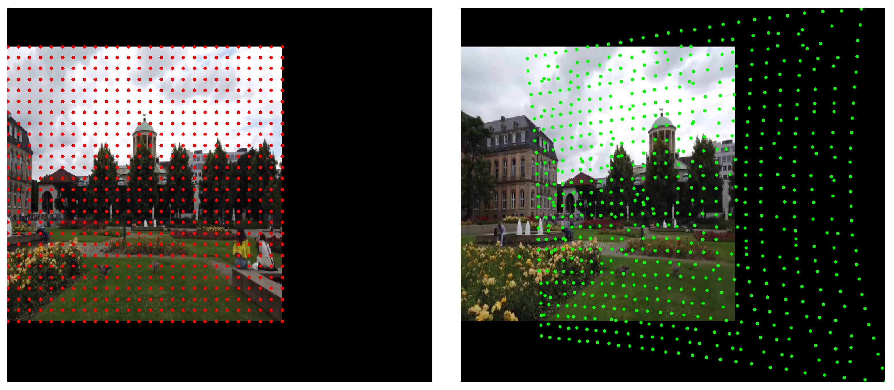
. The red dots in
represent the initial assumption that the feature points are located on the reference image. The green dots in IA indicate the predicted locations of the feature points on the target image, as determined by the network. The yellow dots in
represent the centers of each grid, which are utilized to compute the weight of each feature point within that grid.
is the distorted image of the target image.
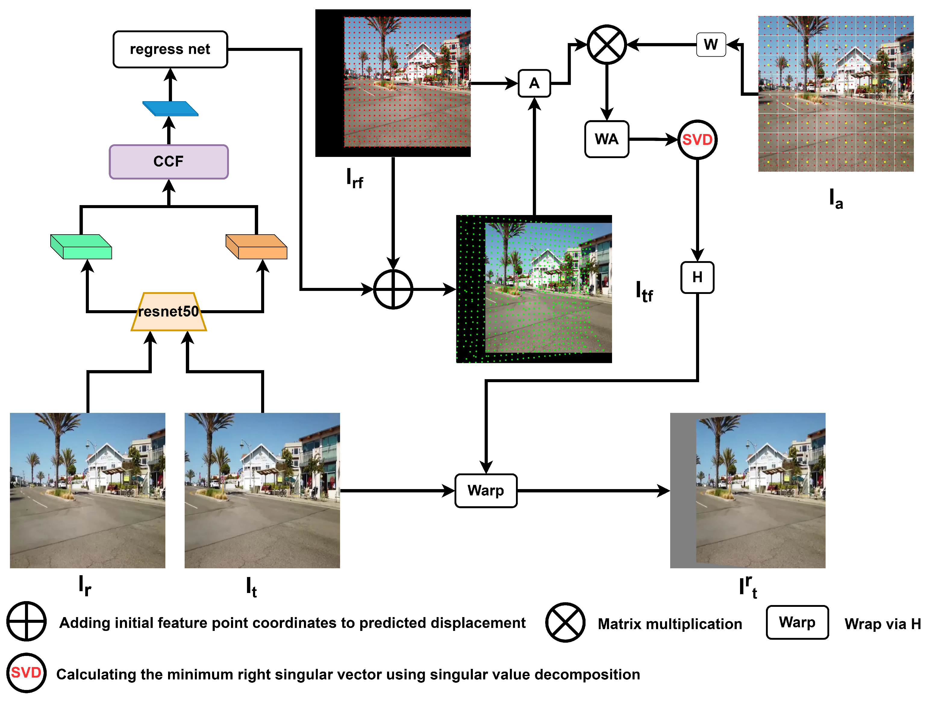
3.3. Chunking and Reverse Distortion
Deep multigrid morphing differs from deep single-grid morphing and image warping using one coordinate transformation formula (e.g., TPS [
13]) in that each pixel in deep single-grid morphing and TPS shares the same warping parameter, whereas deep multigrid morphing requires the assignment of a distinct homography to each pixel within the grid following the morphing process. As illustrated in
Figure 4a, we only assign a homography to the pixel points within the grid after deformation, which correspond to the shape before distortion, as shown in
Figure 4b. In the image, pixel points outside the grid region shown in
Figure 4b could not be used to determine the warping parameters for warping. The determination of the precise area of each pixel block in an image and the performance of pixel interpolation operations on a single image are complicated by the uncertainty of the grid shape. Consequently, it is challenging to generate a comprehensive distorted image by distorting the target image.
To address this issue, it was observed that the monoresponse matrix
H and its inverse matrix
exhibited symmetry during the projection process. This was due to the fact that the transformations applied to the monoresponse matrix and the inverse transformations using its inverse matrix were found to restore the original image to its original state. Moreover, the single response matrix preserves the parallelism of the parallel lines in the image, and the inverse matrix also exhibits this property. Consequently, the inverse of the distortion matrix for each grid can be obtained as
, which represents the multigrid transformation matrix from the reference image
to the target image
. Thereafter, the reference image is partitioned into corresponding blocks in accordance with the shape of the grid divisions, resulting in
. Subsequently, the distorted image blocks of the reference image from the viewpoint of the target image are obtained by applying corresponding distortions to the corresponding blocks. Ultimately, all the distorted blocks are superimposed to obtain the distorted image
.
Once the image
and the target image
have been obtained, the stitched image can be generated through the application of image fusion algorithms, such as the Average Fusion Algorithm and Graphcut Textures [
26]. As illustrated in
Figure 3.
3.4. Loss Function
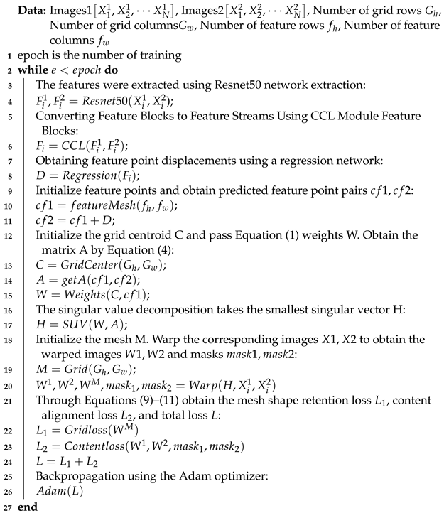
In the context of real-world image stitching networks, current losses can be classified into two categories: content loss and shape-preserving loss. Content loss is employed to regulate the degree of overlap between the constituent image parts, with the objective of optimizing the network. However, relying on content alignment loss alone may potentially lead to the emergence of unnatural mesh distortions, such as self-intersections. It is now necessary to impose constraints by utilizing shape-keeping loss. The shape-preserving loss function correlates neighboring meshes with their surrounding environment, thereby ensuring that all meshes maintain a consistent shape. As our network does not predict the displacements of grid points, but rather the displacements of feature points, we can only solve the distortion matrix of different grids using content alignment loss and inversely warp the grids. As a result, the output image blocks obtained from the inverse warping are not connected to each other (see
Figure 1a,b). To ensure continuity between the image blocks, we introduce a grid shape-keeping loss function
.
In the context of inverse warping, denotes the grid of row i and column j. The subscripts 1, 2, 3, and 4 denote the points on the upper left, upper right, lower left, and lower right of the grid, respectively. Y represents the number of rows of the grid, and X represents the number of columns of the grid. The inclusion of the in Equation (9) serves to prevent singular value decomposition errors during training.
In order to guarantee the efficacy of image alignment effects, it is necessary to utilize the content alignment loss
.
where
represents the distortion operation
B applied to image
A, • denotes the pixel dot product, and
denotes the all-ones matrix. The total network loss is
.
5. Discussion
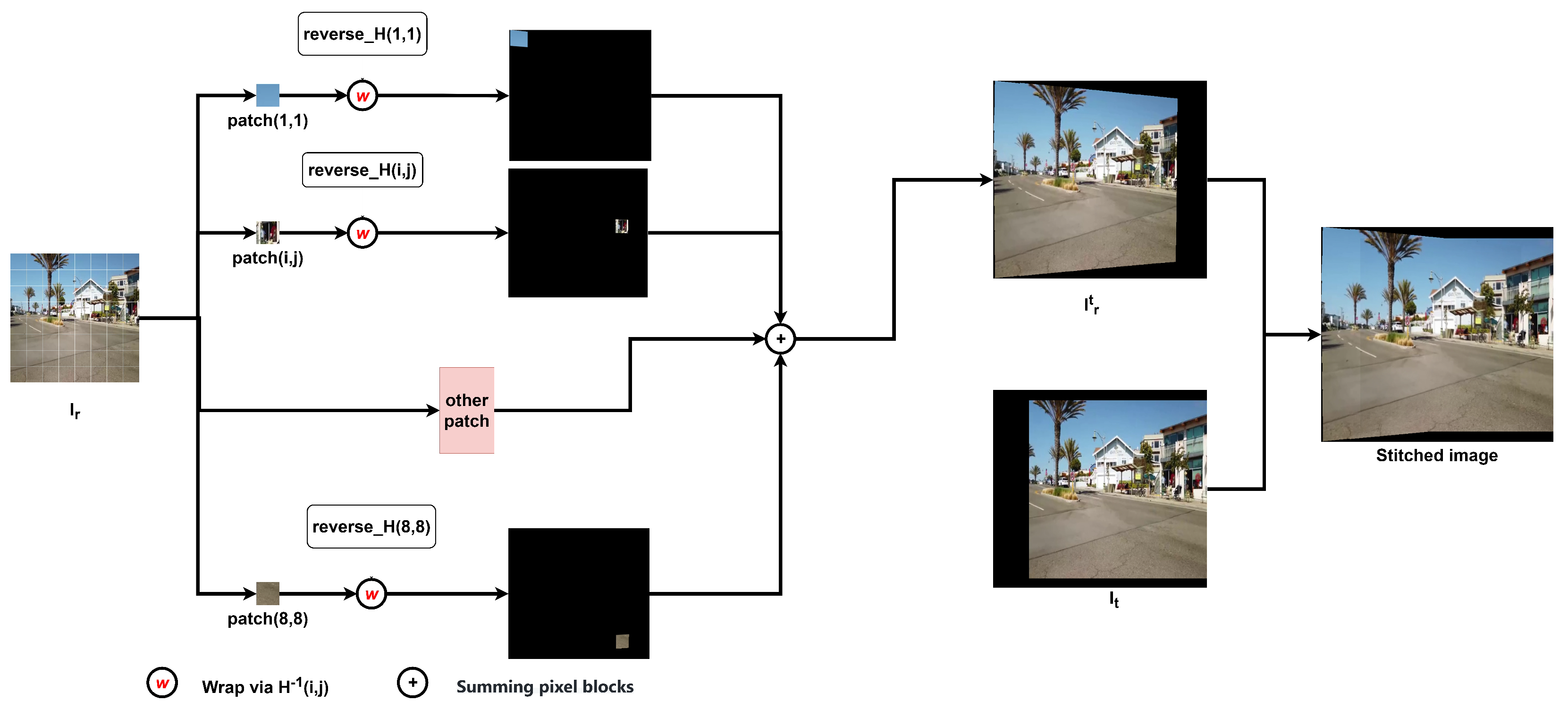
This chapter examines the scalability of the proposed method in terms of alignment performance, processing time, space complexity, the handling of larger datasets, and the ability to accommodate different resolutions. The pseudo-code Algorithm 1 of our network model is also provided at the conclusion of this chapter.
With regard to alignment performance, the method employs a local homography matrix solution based on predicted feature points. While it does enhance grid-based image alignment, it relies on a similar set of feature points to determine the homography, with significant constraints between the local homographies. Consequently, it is unable to distort the image and align in a more flexible manner, as illustrated in
Figure 1a demonstrates that even when no grid constraint loss is applied, the image is naturally distorted to a recognizable degree. Consequently, the image content remains misaligned, even in the presence of significant parallax.
In the future, we intend to address this issue in two ways. One approach is to reduce the constraints between the grids, thereby improving their alignment with the image. Conversely, an alternative approach would be to ascertain whether there exists a superior methodology for partitioning the local distortion space of the image. This could entail the division of disparate distorted image blocks according to their respective objects, with the objective of addressing the issue of large parallax.
In the context of larger datasets, the processing time required is necessarily longer. As the training of the model and the acquisition of the spliced images are conducted as two separate processes, we evaluated both in terms of the time required for training and the time required for acquiring the spliced images with the trained model.
Table 3 illustrates the time required for a single training batch with varying numbers of feature points and grids. It can be observed that the time necessary for a single training session increases gradually with the increase in the number of feature points and grids. Notably, the increase in time associated with an increase in the number of grids is more pronounced.
Table 4 illustrates the time required to obtain a stitched image through chunked reverse warping using the trained model with varying numbers of grids. It can be observed that due to the implementation of warping for each image chunk, the number of warping operations increases with an increase in the number of grids, resulting in a prolonged processing time.
Accordingly, for larger datasets, a smaller number of grids and a reduced number of features may be selected, thereby enabling the stitching results to be obtained in a more expeditious manner.
In terms of space complexity, this study examines the impact of the number of feature points and the number of meshes on the space complexity of the multigrid twisted parameterization module. Let us assume that the number of feature points is M and the number of grids is N. The computational matrix A requires a space of . In the weight computation stage, the requisite space for the weights of each grid is , and the total space required for all N grids is . The matrix requires a space of . The greatest space complexity of the three matrices generated by singular value decomposition SVD is . It is evident that the number of feature points has a more pronounced impact on the computational space resource requirement. Furthermore, an investigation is conducted to ascertain the influence of the number of grids on the space complexity of the chunked inverse warping module. Let us suppose that the image in question has dimensions and that there are N grids. The requisite space complexity for the implementation of chunked reverse warping is . Given that the dimensions of the stitched image are typically greater than those of the input image, the actual space complexity may be somewhat higher than the theoretical value.
Accordingly, in the multigrid distortion parameterization module, the computation of the distortion matrix of a mesh by reducing the number of feature points can effectively reduce the computational space and resource occupation. In the future, an additional optimization may be achieved by solving the distortion matrix of each mesh independently using a small number of feature points. In the case of the chunked inverse warping module, the generation of the stitched image at a significantly faster rate is possible if the warping matrix of each pixel point can be accurately determined at the time of image generation. This may result in an improvement of up to N-fold in the speed of image generation.
At present, our network is only capable of image stitching at a resolution of
pixels. However, in practical applications, it is often necessary to handle images of varying resolutions. As our network is based on feature point displacement prediction, we can scale the image to
pixels, predict the displacement of image feature points, and restore these feature points proportionally. By employing these reduced feature points, the distortion matrix at the original resolution can be calculated, thereby enabling the task of image stitching at different resolutions to be accomplished.
| Algorithm 1: networked algorithmic process |
![Symmetry 16 01064 i001]() |
6. Conclusions
The article presents an innovative approach to image alignment, proposing a novel method for predicting feature point displacements and combining them with traditional feature point-based warping techniques to achieve a more accurate picture alignment process. By assuming a uniform distribution of feature points and using a deep learning network to predict their displacements, we successfully simulate the position of feature points of one image in the viewpoint of another image to achieve robust feature point extraction. Furthermore, we parameterize the APAP algorithm to achieve deep learning APAP multigrid image stitching, thereby obtaining a more accurate alignment of its results. Furthermore, we introduce a post-processing method of multigrid inverse warping and mesh shape preservation loss for the generation of crack-free panoramic images.
The experimental results demonstrate that the proposed method achieves a significant improvement in the image alignment task, indicating potential applications in real-world applications. The combination of deep learning and traditional algorithms enhances the accuracy of the traditional graphic alignment method, thereby providing substantial support and guidance for the resolution of image processing issues in practical applications.


