A Novel Self-Adaptive Deformable Convolution-Based U-Net for Low-Light Image Denoising

Abstract

Capturing images under extremely low-light conditions usually suffers from various types of noise due to the limited photon and low signal-to-noise ratio (SNR), which makes low-light denoising a challenging task in the field of imaging technology. Nevertheless, existing methods primarily focus on investigating the precise modeling of real noise distributions while neglecting improvements in the noise modeling capabilities of learning models. To address this situation, a novel self-adaptive deformable-convolution-based U-Net (SD-UNet) model is proposed in this paper. Firstly, deformable convolution is employed to tackle noise patterns with different geometries, thus extracting more reliable noise representations. After that, a self-adaptive learning block is proposed to enable the network to automatically select appropriate learning branches for noise with different scales. Finally, a novel structural loss function is leveraged to evaluate the difference between denoised and clean images. The experimental results on multiple public datasets validate the effectiveness of the proposed method.

1. Introduction

In the rapidly advancing field of imaging technology, low-light photography presents a unique set of challenges that have attracted the interest of researchers and practitioners. The inherent difficulties in capturing high-quality images under low-light conditions stem from the fundamental limitations of image sensors and the optical properties of the scene being captured [1]. Despite the fact that the human vision system exhibits remarkable adaptability to varying light levels, enabling it to discern details even in near darkness, it is still difficult for digital imaging devices to replicate this capability. This disparity primarily stems from the presence of noise that plagues images when sensors are forced to operate at high gain levels to detect minimal available light [2]. As a result, it not only degrades the aesthetic appeal of the image but also hampers the extraction of meaningful visual information. Although a high ISO can help increase the brightness of an image, it simultaneously amplifies noise. Additionally, a long exposure might induce a blurring effect due to the scene change and camera motion [3,4].

Instead of gathering more light during the image capturing process, another method is to make full use of image-processing techniques to address noise issues in low-light images. Early image denoising methods [5,6,7,8,9] mainly focus on modeling the noise distribution in images. Nevertheless, it is very difficult to model the complex noise distribution generated under natural conditions precisely, which severely affects the denoising effectiveness. In recent years, deep learning [10] has been established as a very powerful tool for feature extraction and has been widely used in multiple research areas such as image classification [11,12,13,14], object detection [15,16,17,18,19], image segmentation [20,21,22,23], etc. By optimizing the feature extractor and classifier in an end-to-end fashion, deep-learning-based methods can automatically extract high-level feature representations and achieve a global optimum during the training process. Deep learning has also been applied in the area of image denoising [24,25,26], especially for low-light conditions [27,28,29,30]. By learning the mapping between the paired data, the low-light noisy image and the corresponding clean image, there has been great progress, and this method has become the mainstream in this field [31,32,33].

However, such a mapping between paired data is very difficult to learn. The first problem is the lack of real paired data. The volume of paired real data is very limited due to the physical environment, which might impede the model optimization and the development of denoising methods, especially for learning-based methods. Many researchers address this problem by generating synthesized data according to noise distribution modeling [34], which can generate noisy and clean image pairs. Nevertheless, some kinds of noises are difficult to accurately model (i.e., read noise); the noise distribution of synthesized data might be very different from real data, leading to invalidation of learned noise models in real-world scenarios [35]. In the last few years, with the emergence of datasets such as SID [36], the volume of paired real data has continued to increase, providing a foundation for optimizing learning-based denoising models.

On the other hand, the extremely complex noise distribution is very difficult to model, which seriously affects performance improvements for learning-based denoising methods. Although multiple learning-based methods have been proposed and have achieved outstanding performances, the majority of work [30,32,35] still focuses on the modeling of the noise distribution during the imaging process rather than improving the ability of modeling the noise distribution. Due to the inability of accurately obtaining a noise distribution model under the current conditions, it is extremely difficult to precisely apply prior noise modeling knowledge with deep learning models. Meanwhile, most existing learning-based methods take advantage of the symmetrical U-Net structure [37] with a $3\ast 3$ convolution kernel, but such a fixed small-size kernel (receptive field) cannot deal with complex noise distributions in images. As a noise pattern is visually represented as patterns with different scales and geometries, it is difficult for a fixed small-size convolution kernel to deal with noise patterns properly, which further limits the ability of modeling and feature extraction in terms of noise. Considering those problems, a novel method is proposed to deal with the low-light image denoising task in this paper, and the main contributions can be summarized in the following:

(1)

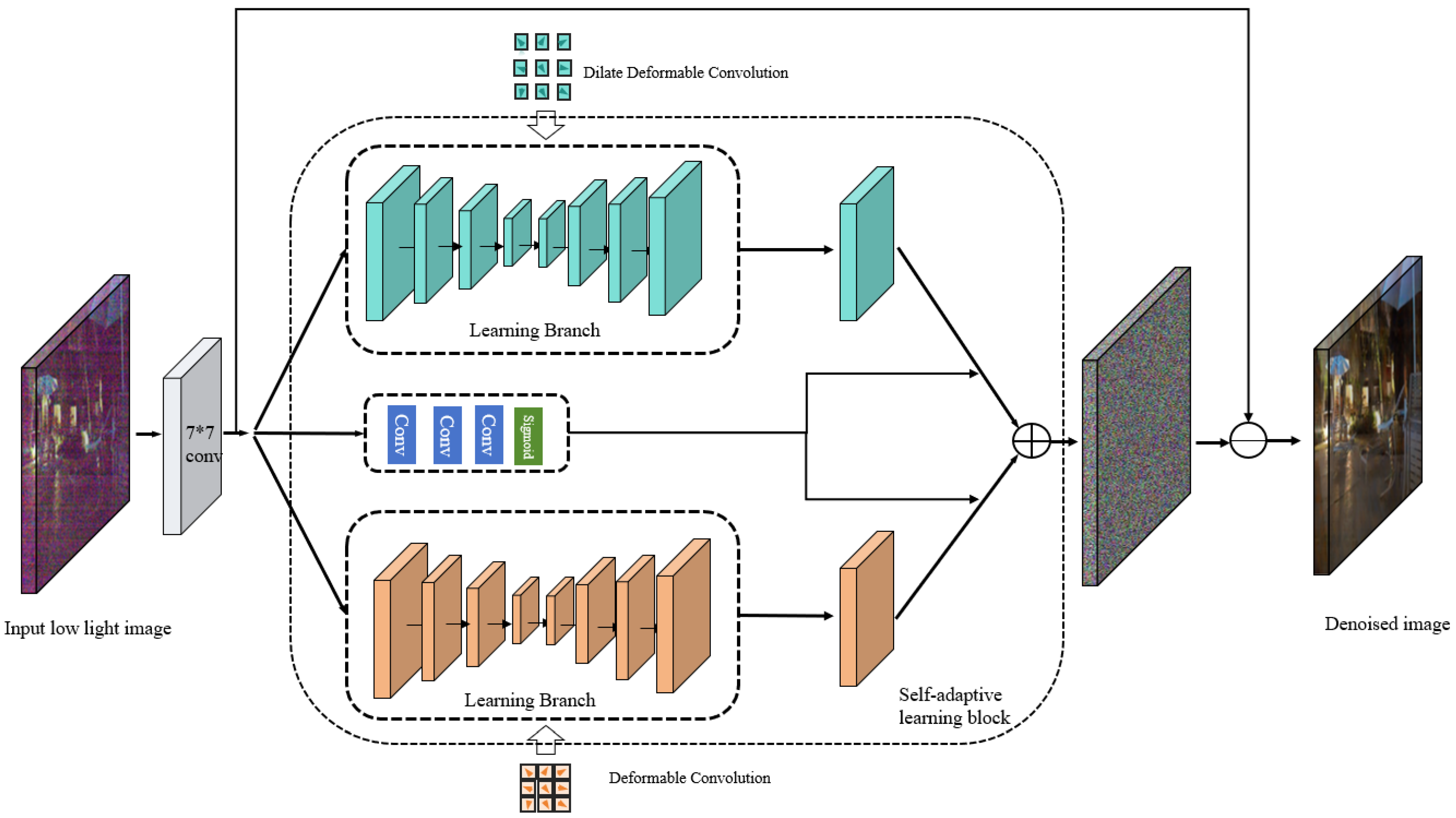
A novel low-light image denoising model termed SD-UNet is proposed to specially address the challenge of low-light image denoising caused by the weak noise distribution modeling ability of existing deep models. The proposed method can extract more reliable noise distribution representations and achieve low-light image denoising effectively.

(2)

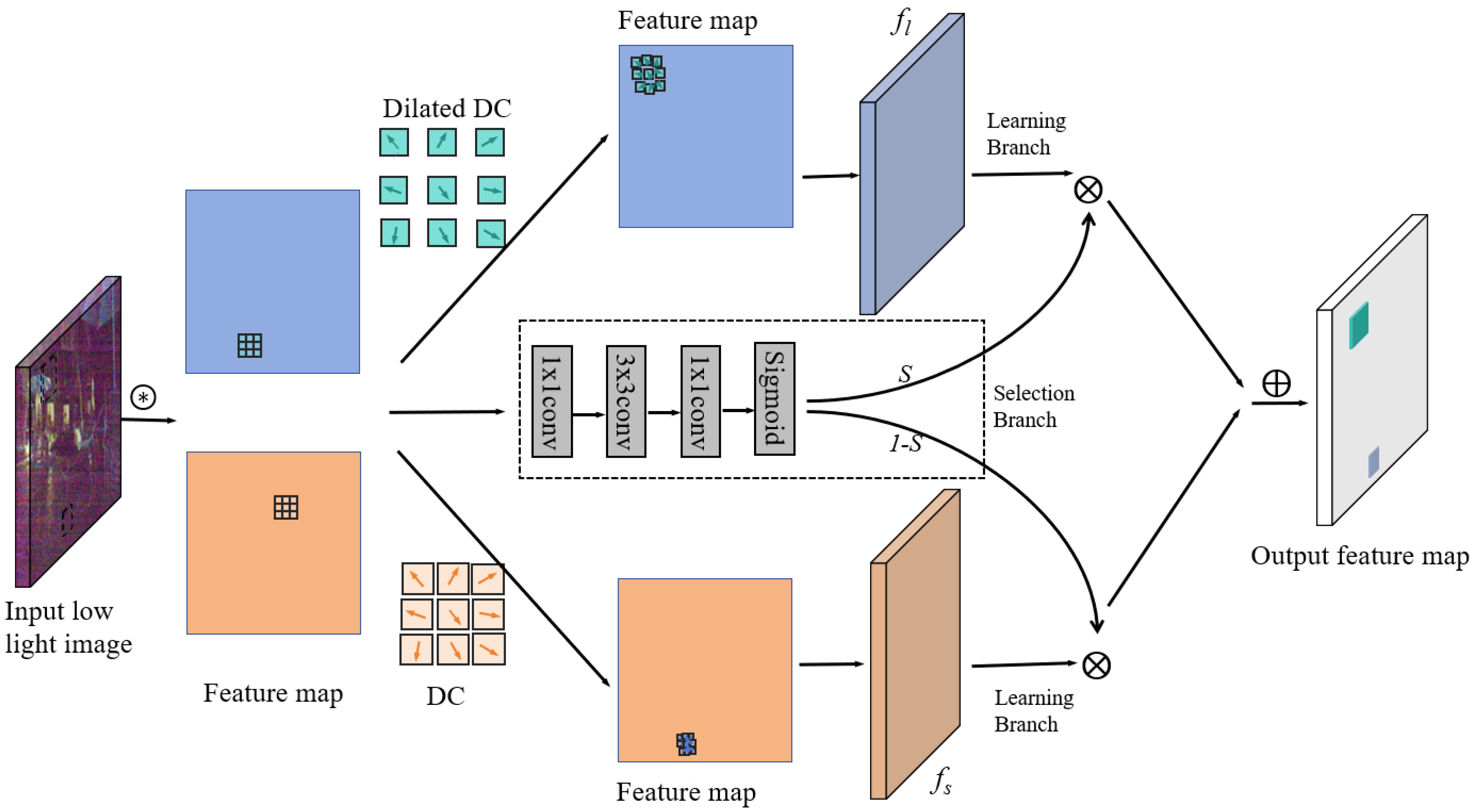
A self-adaptive learning block combined with deformable convolution is leveraged to overcome the limitation of a fixed convolution kernel size. The deformable convolution has a flexible receptive field, and the self-adaptive learning block can enable the network to automatically select a learning branch with an appropriate scale, which will effectively improve the noise feature extraction ability of the proposed SD-UNet.

(3)

A novel structural loss function is proposed to facilitate the parameter optimization process. The proposed loss function can evaluate the difference between a denoised image and the ground-truth clean image more precisely, thus guiding the model parameter optimization process and improving the model’s ability to extract noise distribution more effectively.

The rest of this paper is organized as follows: Section 2 introduces the related work, and Section 3 presents a detailed description of the proposed SD-UNet. Section 4 discusses and analyzes the experimental results, and the whole paper is concluded in Section 5.

2. Related Work

Low-light image denoising is a well-developed topic in the low-level vision research field that has drawn great attention in recent years. Based on the noise modeling method, existing methods can be divided into two categories: physics-based methods and learning-based methods.

2.1. Physics-Based Methods

A physics-based method categorizes sensor noise into two classes: signal-dependent noise and signal-independent noise. The signal-dependent noise is primarily characterized by shot noise, which is usually modeled as a Poisson distribution and influenced by the signal intensity and the camera gain. The camera gain is often achieved by capturing flat-field frames under uniform sensor illumination, followed by the photon transfer method to extract the system gain [26,31,33]. A similar approach termed PMRID [38] uses a sequence of gray-scale chart images to perform system gain calibration through the photon transfer method. The signal-independent noise encompasses a variety of sources, including dark current noise, read noise, row noise, and quantization noise. The parameters associated with these types of noise can typically be extracted by bias frames captured in darkness. To model both read and dark current noise, the ELD method [31] takes advantage of the Tukey lambda distribution [39], which is known for its longer tail that is effective in reducing chrominance artifacts, particularly in low-light conditions. In contrast, the PMN technique [35] focuses solely on modeling dark current fixed-pattern noise. In addition to the dark current fixed-pattern noise, thermal effects within the circuitry can result in black-level error noise. This type of noise is modeled by a uniform distribution [30], either through random sampling from actual data [31] or by averaging a large number of bias frames. Row noise is usually represented by a vector that adheres to a Gaussian distribution [30,40], while quantization noise is mathematically characterized by a uniform distribution.

2.2. Learning-Based Methods

In recent years, with the rapid development of deep learning technology known for its powerful feature extraction, learning-based low-light image denoising methods have became the mainstream in this field. In order to satisfy the requirement of a sufficient number of real image pairs for the optimization of learning-based methods, Chen et al. [36] propose a novel SID dataset which contains a sufficient number of real image pairs. Meanwhile, it applies a U-Net model to deal with the low-light image denoising task, achieving an outstanding performance. Wei et al. [31] propose a physics-based noise model for extreme low-light photography; its performance is comparable to that of models trained with paired real data. NoiseFlow [41] applies a flow-based model that maximizes the likelihood of sampled noise. CA-GAN [42] feeds the clean image and a random Poisson–Gaussian noise into a generator to produce the synthetic noise; Cycle-GAN [43] is an unsupervised generative adversarial network that has been widely used in the cross domain translation area and has shown outstanding performance on night-to-day image translation tasks. ToDayGAN [44] is one of the state-of-the-art (SOTA) methods that deals with low-light image enhancement by generating fake night-time images and distinguishing between real and fake night-time images. Pixel2Pixel [45,46] leverages the U-Net structure to generate outputs with the same size of input, and the combination of L1 loss and contrastive loss is utilized to promote parameter optimization. Zamir et al. [47] constructed a multi-scale residual block that contains several key elements to enable a network to maintain spatially precise high-resolution representations through the entire network and to obtain useful contextual information from the low-resolution representations, which achieved outstanding performance on multiple image enhancement tasks. Starlight adopts a more demanding setting under starlight, yet the performance is still limited and the fixed-pattern noise needs to be hand-calibrated. Feng et al. [35] propose a learnability enhancement strategy to reform paired real data according to noise modeling, which achieved an outstanding performance in low-light image denoising.

As mentioned above, existing learning-based methods still focus on applying the prior noise distribution knowledge into the deep learning model while ignoring the analysis of model characteristics and the improvement in the noise modeling ability. Given the problems of existing studies, this paper proposed an SD-UNet for the low-light image denoising task, which is validated on the SID [36] and ELD [31] datasets that contain a sufficient number of noisy and corresponding real image pairs.

3. SD-UNet

In this part, the overall network architecture of the proposed SD-UNet is firstly described in Section 3.1. The detailed implementation of the deformable convolution and self-adaptive learning block is then demonstrated in Section 3.2 and Section 3.3, respectively. The structural loss function is briefed introduced in Section 3.4.

3.1. The Overall Structure of SD-UNet

The overall structure of the proposed SD-UNet is shown in Figure 1, which consists of three parts: (a) the residual U-Net structure, (b) the deformable convolution and (c) the self-adaptive learning block. The raw low-light noisy image first goes through a convolution layer with a kernel size of $7\ast 7$; the large kernel size allows the network to learn more comprehensive feature representations of the input image. After this, the output feature map goes through the self-adaptive learning block which contains two learning branches and a selection branch, where each learning branch is a U-Net structure constructed by a stack of convolution layers and deconvolution layers with deformable convolution. The outputs from each learning branch are then fused by the guidance from the selection branch. The output feature maps $F_S$ are then concatenated with the initial input feature map $F_I$ to form the final denoised image $F_D$. The final denoised image can be calculated as:

$$F_D=F_I-F_S.$$

(1)

Such a residual structure guarantees that the proposed network structure focuses on learning the noise representation, thus further enhancing the noise modeling ability.

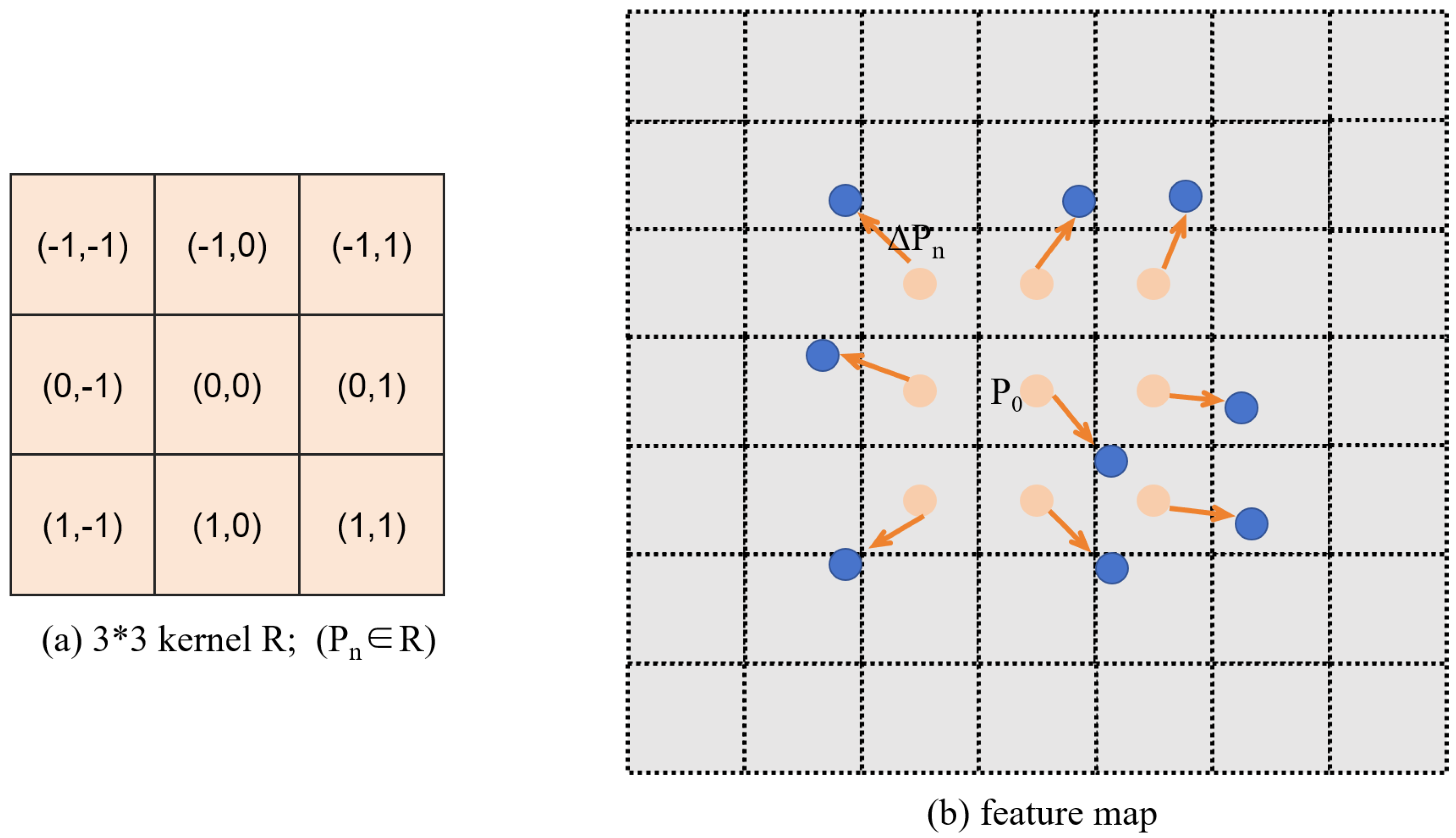
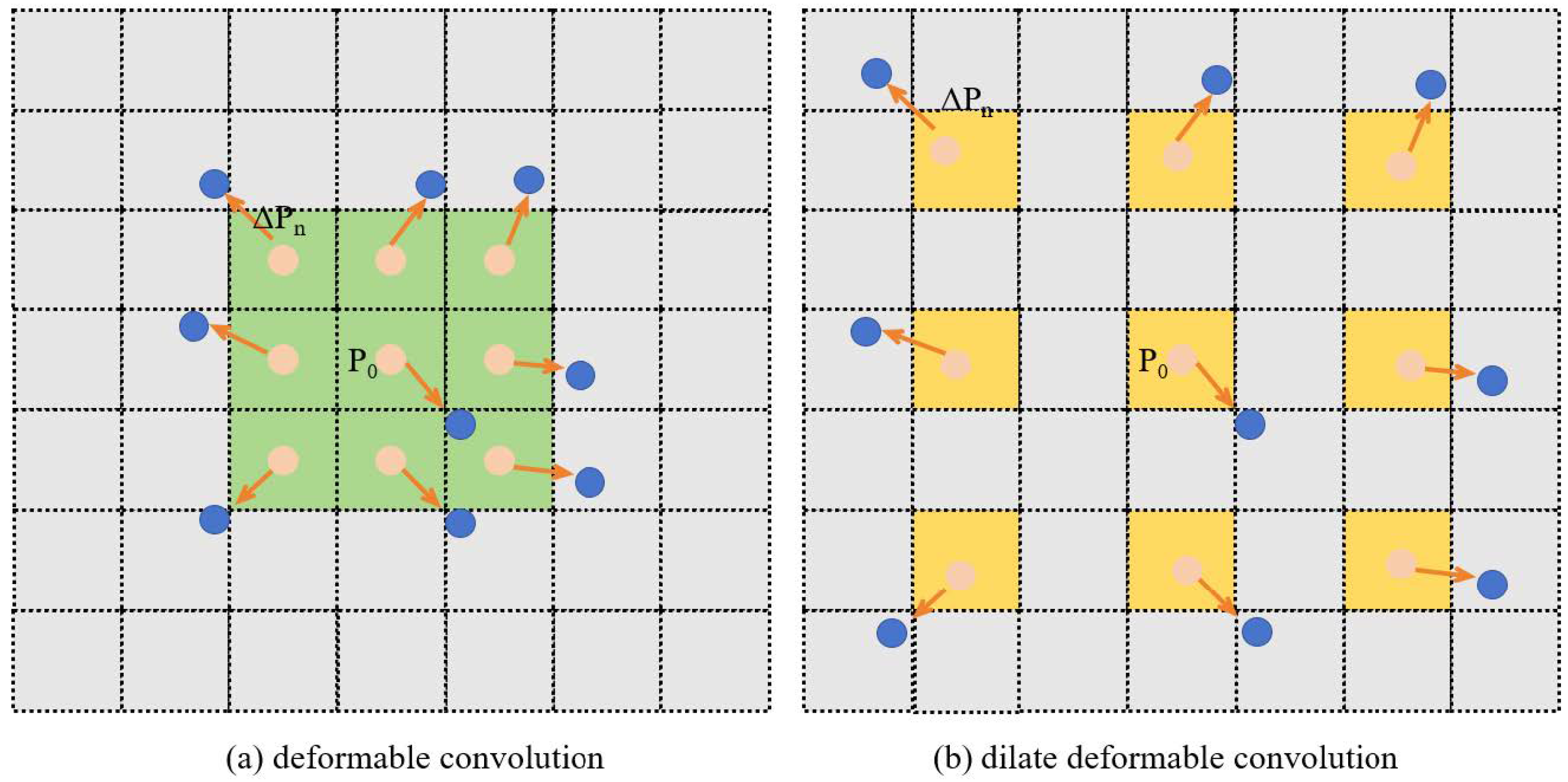
3.2. Deformable Convolution

The noise within an image is often visually represented as patterns with a different geometry, which makes it hard for existing deep models with a fixed-size convolution kernel to extract reliable noise feature representations. Compared with the traditional operation, the deformable convolution has a much more feasible receptive field for extracting dense spatial transformations.

Mathematically, the specific operation of deformable convolution can be defined as follows:

$$y\left(p_0\right)=\sum _{p_n\in \mathcal{R}}w\left(p_n\right)·x\left(p_0+p_n+\Delta p_n\right)$$

(2)

where $P_0$ means the location of the output feature map and $y\left(p_0\right)$ represents the value of position $P_0$ on the output feature map. In the traditional convolution operation, $y\left(p_0\right)$ is accumulated by multiplying the pixels at a fixed position on the input feature map and the corresponding position weight of the convolution kernel. However, due to the offset in deformable convolution, the value of this position will be calculated according to the offset position in the deformable convolution. ${\sum }_{p_n\in \mathcal{R}}$ represents the summation of all positions $P_n$ in the convolution kernel. R means the coverage of the convolution kernel which is all possible relative positions within the convolution kernel. $w\left(p_n\right)$ is the weight of the convolution kernel at position $P_n$. $x\left(p_0+p_n+\Delta p_n\right)$ represents the sampled value after offset on the input feature map. $\Delta P_n$ is the offset learned by the additional convolution in deformable convolution. Its size is the same as the input feature map, but the number of channels is $2N$ (N is the size of the convolution kernel), which represents the offset in the x and y directions, respectively. This is the main difference between deformable convolution and the traditional convolution operation. The original convolution sampling position is changed by the offset $\Delta P_n$, which can be seen in Figure 2.

It is obvious that the deformable convolution kernel can achieve different shapes of receptive fields under the same weight parameters. This enables the deformable convolution kernel to acquire a certain adaptive ability and dynamically adjust its shape and size according to the content and structure of the noise in the input image. Specifically, the deformable convolution kernel usually contains two parts of parameters: local offset parameters and convolution weight parameters. The local offset parameter is used to control the position and shape of the convolution kernel on the input feature map, while the convolution weight parameter is used to perform convolution operations on the input feature map. By learning these parameters, the deformable convolution kernel can dynamically adjust its shape and size according to different regions of the input feature map, thereby achieving flexible shapes of receptive fields. Therefore, even if the convolution kernels of the two learning branches have the same weight that show approximately symmetrical in structure, different noise features can be extracted based on the offset range of different convolution sampling positions. This enables the network to improve its ability to deal with noise patterns of various sizes and deformable geometries without requiring additional weight parameters. As a result, only one deformable convolution kernel with two different constrained offsets is necessary to achieve this effect.

3.3. Self-Adaptive Learning Block

Despite the fact that deformable convolution can deal with noise patterns much better, it still fails to fit noise patterns with different scales very well as the offset of deformable convolution is limited to 1 pixel. In this paper, a novel self-adaptive learning block (SALB) is also proposed to tackle different scales. The structure of the proposed SALB is shown in Figure 3.

The proposed SALB contains three branches, including two learning branches and one selection branch. Each learning branch tackles a different scale by utilizing convolution kernels with different sizes. During this process, a novel dilated convolution is proposed to deal with large-scales patterns by enlarging its receptive field while not increasing the number of parameters and computation costs. Therefore, the self-adaptive learning branch structure can deal with large-scale and small-scale noise patterns at the same time. As shown in Figure 4, the dilated deformable kernel presents a bigger receptive field compared with the traditional deformable convolution operation, so the dilated deformable convolution can handle large-scale noise patterns more effectively.

By taking advantage of deformable convolution and dilated deformable convolution, the two learning branches in the SLAB can deal with noise patterns with different scales much better. Each learning branch contains a U-Net structure similar to paired data (SID) [36]. The U-Net structure [37] allows the network to extract the high-level semantic representation and then reconstruct a same-size feature map with the input image. As a result, the combination of U-Net and deformable convolution leveraged in this paper can effectively model the noise distribution.

Another branch is termed the selection branch; it enables the model to automatically select appropriate learning branches and fuse the output feature map from two learning branches. The proposed selection branch is composed of a $3\ast 3$ convolution layer, two $1\ast 1$ convolution layers and a sigmoid function. The first $1\ast 1$ convolution is used to reduce the dimension of the feature map and further reduce the number of parameters. Then, after extracting features through a $3\ast 3$ convolution, the shape of the feature map is recovered through a $1\ast 1$ convolution to facilitate the combination of the feature maps from the two different convolution branches. After passing the sigmoid function, a probability value in the range of 0–1 can be calculated for each channel of the final feature map. For each channel, a sigmoid function is applied to generate a score in the range of (0,1) for each pixel in the feature map, and the output for each channel is acquired by calculating the max of all outputs from the corresponding feature map. So, for a k-channel feature map, a k-dimension weight vector is also acquired. The final output score S is acquired by calculating the average of all values corresponding to each channel. The output feature maps of two learning branches are represented as $f_l$ and $f_s$, respectively, and the probability value of the sigmoid function is represented as S. The select operation assigns S and ($1-S$) to $f_l$ and $f_s$ by dot multiplication. At last, the processed $f_l$ and $f_s$ are added to obtain the fused output feature map. This module can be described as Equation (3):

$$\begin{array}{cc}\hfill Output& =S\left(x\right)·f_l(x,w)+(1-S\left(x\right))·f_s(x,w)\hfill \end{array}$$

(3)

The final output from the selection branch can be used to help a network deal with noise with different sizes automatically. If the noise pattern is large, the value of S will be larger; that is, the probability value assigned to the output of the dilated deformable convolution branch is greater than the probability value assigned to the output of the original deformable convolution branch. The parameters of the whole network can be optimized jointly during the training process in an end-to-end fashion, including parameters in the selection branch (parameters in the $3\ast 3$ convolution layer and two $f_l$ layers).

3.4. Structural Loss Function

Previous methods mainly take advantage of the L1 loss to evaluate the difference between a denoised image and a clean image. Such a difference can be further used to guide the optimization process of the proposed method. However, the loss function cannot evaluate the difference precisely as it ignores the whole structure of the image. To this end, a novel structural loss function is leveraged to help evaluate the denoising performance more precisely. The proposed structural loss function is calculated by a combination of PSNR loss, SSIM loss, and canny edge [48]-based structural loss.

As the existence of noise might seriously affect the edge detection performance, the canny-operator-based edge detection performance is used to evaluate the denoising performance of the proposed method. The structural loss function $L_S$ can be calculated as:

$$\begin{array}{c}\hfill L_S=\left|\right|Canny\left(I_D\right)-Canny\left(I_G\right){\left|\right|}_1\end{array}$$

(4)

where $Canny$ means the canny-operator-based edge detection result, $I_D$ means the denoised image, and $I_G$ means the clean ground truth image. The final loss function can be calculated as follows:

$$\begin{array}{cc}\hfill L& =k_1\ast L_P+k_2\ast L_M+k_3\ast L_S\hfill \end{array}$$

(5)

where $L_P$ means the PSNR loss, $L_M$ means the SSIM loss and $L_S$ means the structural loss. $k_1,k_2,k_3$ are weights that can balance the three losses. The final loss function L is then calculated to guide the model parameter optimization process.

4. Experiments

This section presents the results of extensive experiments conducted on multiple public datasets that contain a sufficient number of paired images, including SID [36] and ELD [31]. The efficacy of the proposed model is rigorously assessed through a comparative analysis with the SOTA methods, as described in Section 4.2. Furthermore, the impact of key model components is investigated in the ablation study, expounded upon in Section 4.3. Section 4.4 shown the effectiveness of the proposed structural loss function. Section 4.5 describes the generalization experiment on different dataset to demonstrate the good generalization of the proposed model. Section 4.6 provides an insightful analysis of the model’s performance through visualizations, offering a comprehensive understanding of its effectiveness in low-light image denoising.

4.1. Experiment Details

Datasets: To evaluate the effectiveness of the proposed model, two public low-light image denoising datasets, SID [36] and ELD [31], are introduced to evaluate the performance. Each dataset contains multiple paired images to help the network learn the mapping between low-light noisy and clean images.

SID consists of 5094 short-exposure raw images captured under low-light conditions, and each low-light image has a corresponding normal-light reference image. In addition, it contains indoor and outdoor images, and the outdoor images are usually captured under moonlight or street lighting conditions. Images in the SID dataset are captured by two different cameras, Sony $\alpha$7S and Fuji film X-T2 that are both assembled in Japan, which can be divided into two subsets: $I{D}_{Sony}$ and $SI{D}_{Fuji}$.

ELD covers 10 indoor scenes captured by four Japanese camera devices (SonyA7S2, NikonD850, CanonEOS70D and CanonEOS700D). It has three levels (800, 1600, 3200) and two low-light factors (100, 200) for noisy images, resulting in 240 (3 × 2 × 10 × 4) raw image pairs in total.

Evaluation metrics: In low-light image denoising tasks, the peak signal-to-noise ratio (PSNR) and structural similarity (SSIM) [49] are widely used as evaluation indexes, and are also used in this work.

The PSNR indicates the ratio between the maximum power a signal can reach and the noise power that can affect it. The calculation method can be formed as:

$$PSNR(I,R)=10lo{g}_{10}\left[\frac{{(2^L-1)}^2}{MSE(I,R)}\right]$$

(6)

where $MSE$ is the mean squared error. The $MSE$ can be calculated as:

$$MSE(I,R)=\frac{1}{mn}\sum _{i=1}^m\sum _{j=1}^n\left|\right|I(i,j)-{R(i,j)\left|\right|}^2$$

(7)

where I is an image captured under normal light conditions, R is an enhanced image, L is the largest gray level, and its value is $2^n-1$, and n is the number of pixel bits. A greater PSNR indicates a better enhancement result.

The SSIM is used to evaluate the similarity between two images, and its value ranges from −1 to 1. A large value indicate that the enhanced image is more structurally similar to the image captured under normal light conditions. It is measured from three aspects: brightness, contrast and structure. The SSIM between image I and R can be calculated as:

$$\begin{array}{c}\hfill SSIM(I,R)=\frac{(2{\mu }_I{\mu }_R+c_1)(2{\delta }_{IR}+C_2)}{({{\mu }_I}^2+{{\mu }_R}^2+C_1)({{\delta }_I}^2+{{\delta }_R}^2+C_2)}\end{array}$$

(8)

Experiment Setup: The raw image pre-processing method used in this paper is similar to the ELD dataset. The proposed SD-UNet module is compared with several SOTA modules including Paired Data [36], Poisson–Gaussian (P-G) [9], ELD [31], SFRN [26], Noise Flow [41], MiRNet [47] and PMN [35]. The proposed method is performed on four NVIDIA Tesla T4 graphics cards. More detailed information about the configuration parameters used in the experiment is shown in

Table 1. Experiment setup.

Configuration Item	Value
Central processing unit	Intel(R) Xeon(R) CPU E5-2650 v3
Graphics processor unit	NVIDIA Tesla T4 16 GB
Operating system	Ubuntu 18.04.2 LTS (64-bit)
Memory	128 GB
Hard Disk	2 TB

. All models are implemented in Pytorch and optimized by the Stochastic Gradient Descent Adam optimizer [50] with a momentum of 0.9, a mini-batch size of 4, and a weight decay of $1\times {10}^{-5}$. The initial learning rate was set to $1\times {10}^{-4}$ and decreased every 700 epochs. All models were trained from scratch for 2100 epochs on four GPUs.

4.2. Comparison with SOTA Methods

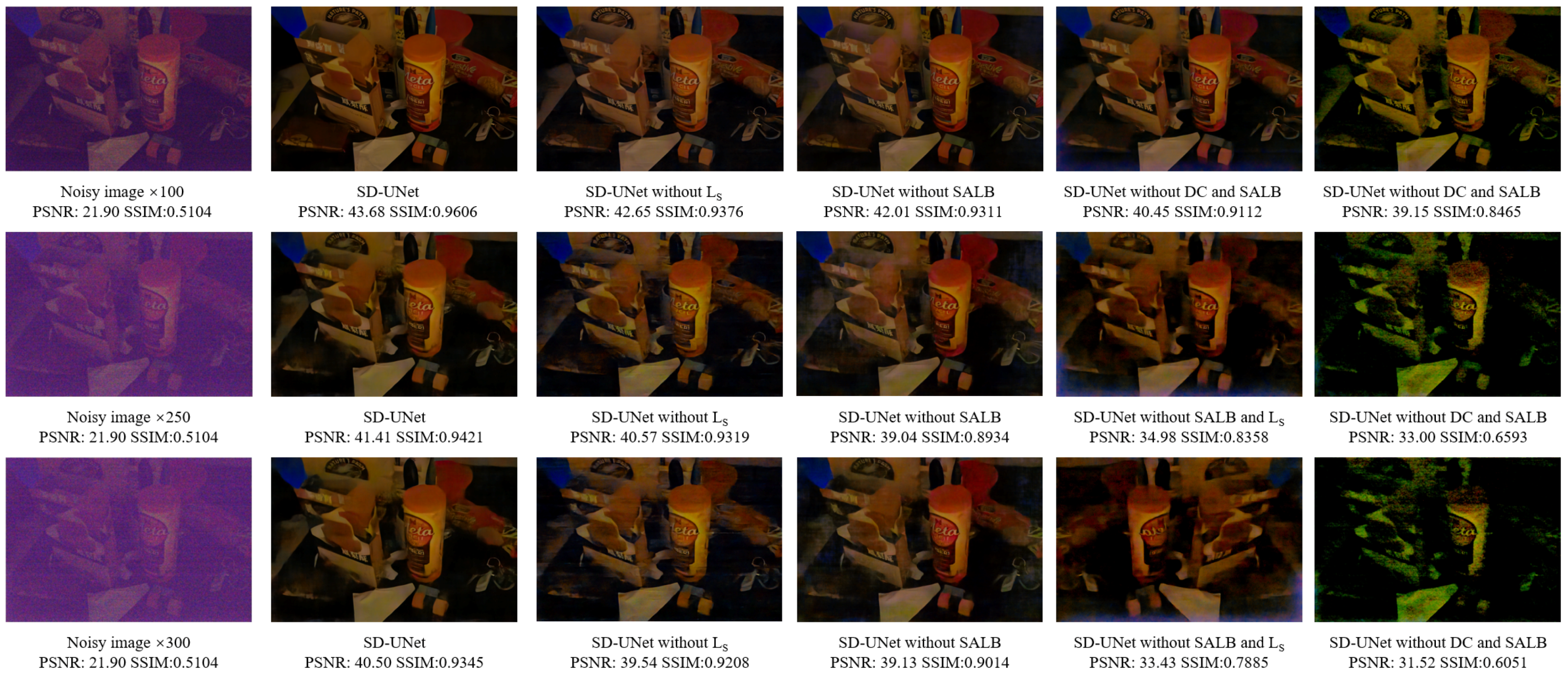
The proposed SD-UNet method is first applied on the SID dataset as it contains a sufficient number of paired real images. So, the proposed method is first applied to the Sony dataset, which was constructed based on three different low-light factors. The above low-light factors correspond to different exposure times; ×100, ×250 and ×300 correspond to 1/10 s, 1/25 s and 1/30 s, respectively. So, the low-light denoising performance on three factors Multiple existing low-light image denoising methods are used to compare with proposed SD-UNet, the quantitative results are shown in

Table 2. The performance comparison between SD-UNet and SOTA methods on the SID Sony dataset.

Method	×100		×250		×300
	PSNR	SSIM	PSNR	SSIM	PSNR	SSIM
P-G [9]	39.03	0.926	35.57	0.861	32.26	0.781
Noiseflow [41]	41.08	0.923	36.90	0.836	32.38	0.753
Paired Data [36]	42.03	0.953	39.57	0.937	36.57	0.922
ELD [31]	41.95	0.953	39.44	0.931	36.36	0.911
MiRNet [47]	41.27	0.949	38.74	0.927	36.08	0.897
SFRN [26]	42.31	0.955	39.60	0.938	36.85	0.923
PMN [35]	43.16	0.960	40.92	0.947	37.64	0.934
SD-UNet	42.79	0.958	40.04	0.941	36.98	0.926

The bold red numbers represent the best value, blue numbers represent the second-best values and green numbers represent the third best values.

.

One can easily see that the proposed SD-UNet can achieve an outstanding performance in low-light image denoising. Compared with paired data, which only takes advantage of a U-Net structure model, SD-UNet can achieve improvements in both PSNR and SSIM, which establishes the effectiveness of the proposed method. Also, compared with methods such as ELD and PMN, the proposed SD-UNet can still achieve a very promising denoising performance, while it avoids requiring much prior knowledge of the noise distribution, highlighting that the proposed deep network has a higher noise modeling ability compared with traditional deep network structures. In addition, SD-UNet can achieve denoising performance improvement on all three low-light factors, which means that it can be used for images with different levels of noise, thus further establishing its generalizability. It is worth noting that although the PMN method achieves the best performance, it requires not only paired images, but also a large number of bias and flat field frames.

The distributions of PSNRs and SSIMs of the SID dataset are also shown in Figure 5, where red dots represent images captured under 1/10 s, green dots represent images captured under 1/25 s and blue dots represent images captured under 1/30 s. One can easily see that images captured at longer exposure times have higher PSNR and SSIM values, which means that these images are more easily denoised.

4.3. Ablation Study

In order to further evaluate the effectiveness of each component proposed in this paper, a further detailed ablation study is also performed. The results of the ablation study are shown in

Table 3. The ablation study of SD-UNet.

DC	SALB	${\mathit{L}}_{\mathit{S}}$		×100	×250	×300
✓			PSNR	42.33	39.72	36.75
			SSIM	0.955	0.938	0.922
		✓	PSNR	42.18	39.65	36.60
			SSIM	0.956	0.941	0.924
✓	✓		PSNR	42.51	39.91	36.90
			SSIM	0.956	0.939	0.923
✓		✓	PSNR	42.38	39.88	36.83
			SSIM	0.957	0.941	0.926
✓	✓	✓	PSNR	42.79	40.04	36.98
			SSIM	0.958	0.941	0.926

The red numbers represent the best values.

. An ablation study was also performed on the SID Sony dataset.

From the ablation study results, one can easily see that the proposed components can lead to improvements in the final denoising performance. Firstly, one can see that deformable convolution can improve the final denoising performance, which means the deformable-convolution-based method has a higher noise distribution modeling ability, which makes it achieve significant improvements in both PSNR and SSIM. The proposed structural loss function $L_S$ can guide the optimization process and help the network retain more reliable structural information, leading to significant improvements in the SSIM. The SALB is not performed alone, as it should be used with deformable convolution. By adding an SALB, the denoising performance is improved and the effectiveness of the proposed SALB can be established. The difference in performance between leveraging both deformable convolution and the SALB and only using DC highlights that the proposed self-adaptive learning scheme can help improve the denoising performance, which proves the effectiveness of the proposed SALB.

Thus, by removing any module alone, the corresponding denoising performance is reduced, so the three parts are indispensable and complement each other, resulting in the best effect. In addition, in order to show the effectiveness of the proposed method, a visual comparison was also conducted. The visual comparison is shown in Figure 6, where the same picture captured with different exposure times is shown and the denoised images generated by SD-UNet and the other methods in Table 2 are shown. Moreover, the PSNR and SSIM value for each denoised image is shown below each corresponding image.

In Figure 6, one can see the effectiveness of the three parts proposed in this paper. The SD-UNet without the SALB achieved quite a poor performance, and the denoised image exhibits very serious color distortion and blurring. So, the proposed SALB helped model the noise distribution more precisely. Also, the proposed $L_S$ loss can also help the network maintain spatial structure information, which represents an improvement over SSIM. Also, by a comparison of the performance of SD-UNet without deformable convolution and the SALB and SD-UNet without the SALB, one can see that the PSNR and SSIM significantly improved by applying deformable convolution, and the denoised image shows significant improvement and has a more precise color distribution and texture. So, the effectiveness of the three proposed components in this paper has been established.

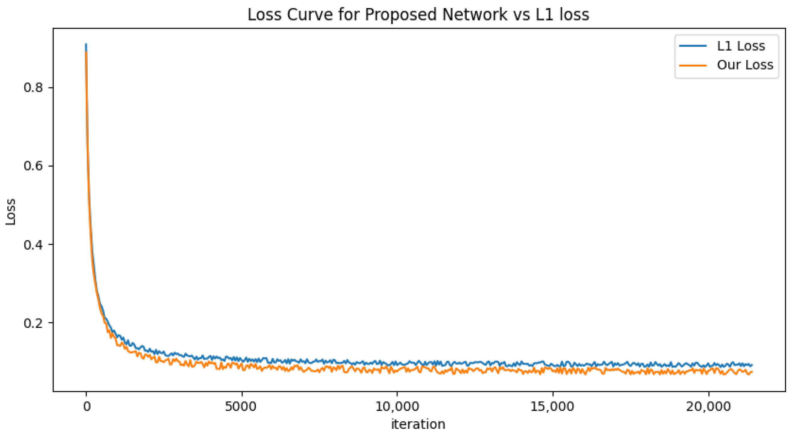
4.4. The Effectiveness of the Proposed Loss Function

In order to further evaluate the effectiveness of the proposed structural loss function, a further comparison is conducted on the SID dataset, and this comparison is detailed in this subsection. The widely used L1 loss is used to compare the proposed structural loss function; the experiment results are shown in

Table 4. The performance comparison between the proposed loss function with L1 loss on the SID Sony dataset.

Method	×100		×250		×300
	PSNR	SSIM	PSNR	SSIM	PSNR	SSIM
$L_S$ Loss	42.79	0.958	40.04	0.941	36.98	0.926
L1 Loss	42.53	0.931	40.03	0.925	36.71	0.912
L1+$L_S$ Loss	42.77	0.959	0.942	0.959	36.96	0.927

The red number represents for the best values.

and the training curves are also shown in Figure 7.

One can see from Table 4 that the proposed structural loss shows better performance than the L1 loss function, while it exhibits a very competitive performance with $\mathrm{L}1+L_S$ loss. This is because the proposed $L_S$ loss can help maintain the spatial structure during the denoising process, which leads to performance improvements over L1 loss, especially on SSIM. In addition, as shown in Figure 7, one can see that the training curve of the proposed loss exhibits significantly lower training loss values than the L1 loss, with the proposed method’s loss value decreasing faster and more smoothly, which further establishes the effectiveness of the proposed structural loss function.

4.5. Further Experimental Results on the ELD Dataset

In order to evaluate the robustness of the proposed method, a further experiment was also conducted on the ELD dataset, which contains paired images from four cameras. In this paper, the experiment is conducted on two models: a Sony A7S2 Camera and a Nikon D850 Camera. For each camera, two low-light factors are used in the image capturing process, ×100 and ×200, which correspond to different exposure times. So, a denoising performance comparison is conducted between the proposed SD-UNet and multiple SOTA methods. The results are shown in

Table 5. The performance comparison between SD-UNet with SOTA methods on the ELD dataset.

Method	Sony A7S2				Nikon D850
	×100		×200		×100		×200
	PSNR	SSIM	PSNR	SSIM	PSNR	SSIM	PSNR	SSIM
P-G [9]	41.72	0.925	39.27	0.870	41.68	0.907	39.99	0.887
Noiseflow [41]	41.05	0.924	39.23	0.889	41.55	0.881	38.95	0.820
Paired Data [36]	44.43	0.964	41.95	0.927	43.01	0.950	41.10	0.926
ELD [31]	45.40	0.971	43.41	0.954	42.85	0.949	41.08	0.928
MiRNet [47]	44.83	0.967	42.17	0.932	42.34	0.938	40.47	0.919
SFRN [26]	45.74	0.976	43.84	0.955	43.04	0.949	41.28	0.930
PMN [35]	46.50	0.985	44.51	0.973	43.28	0.960	41.32	0.941
SD-UNet	45.83	0.979	43.67	0.948	43.18	0.952	41.27	0.931

The bold red numbers represent the best value, blue numbers represent the second-best values and green numbers represent the third best values.

.

From the experimental results, one can easily see that the proposed SD-UNet can still achieve a competitive performance on the ELD dataset, as well as with different image capturing equipment, which shows that SD-UNet can be applied to different datasets and different camera equipment. By comparing the proposed SD-UNet and paired data, the proposed SD-UNet can achieve performance improvements for each index, which shows that the proposed model has a better noise modeling ability. By comparing the performance of the proposed method on different factors, it can still achieve performance improvement on images captured with different exposure times, which effectively shows the generalizability of the proposed method.

The PSNR and SSIM distributions on the ELD dataset are also shown in Figure 8, where red dots represent images captured under 1/10 s and green dots represent images captured under 1/20 s. Similar to the SID dataset, one can easily see that images captured at longer exposure times have a higher SSIM value, while some of the images failed to achieve a high PSNR value. This may because the proposed method can fit the SSIM much better, which means that the proposed method can better maintain the structure of objects and better replicate the visual effects of the human eye.

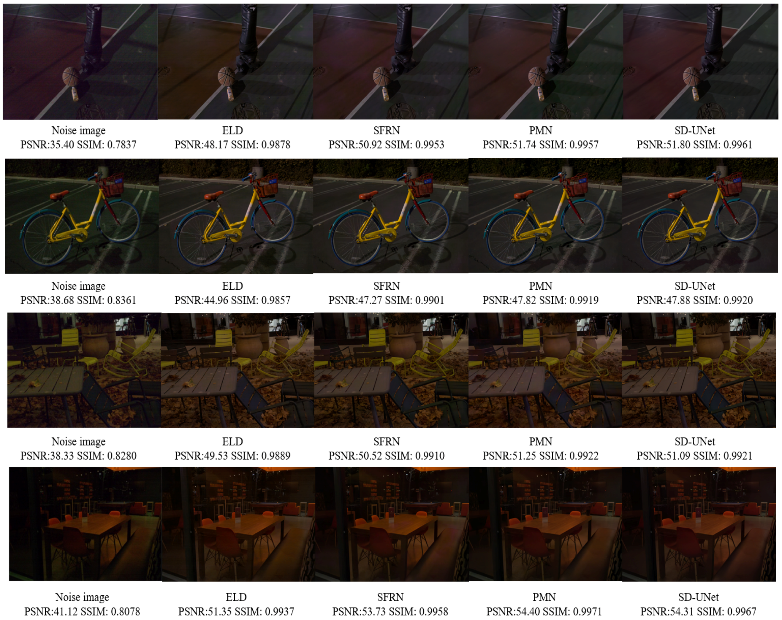
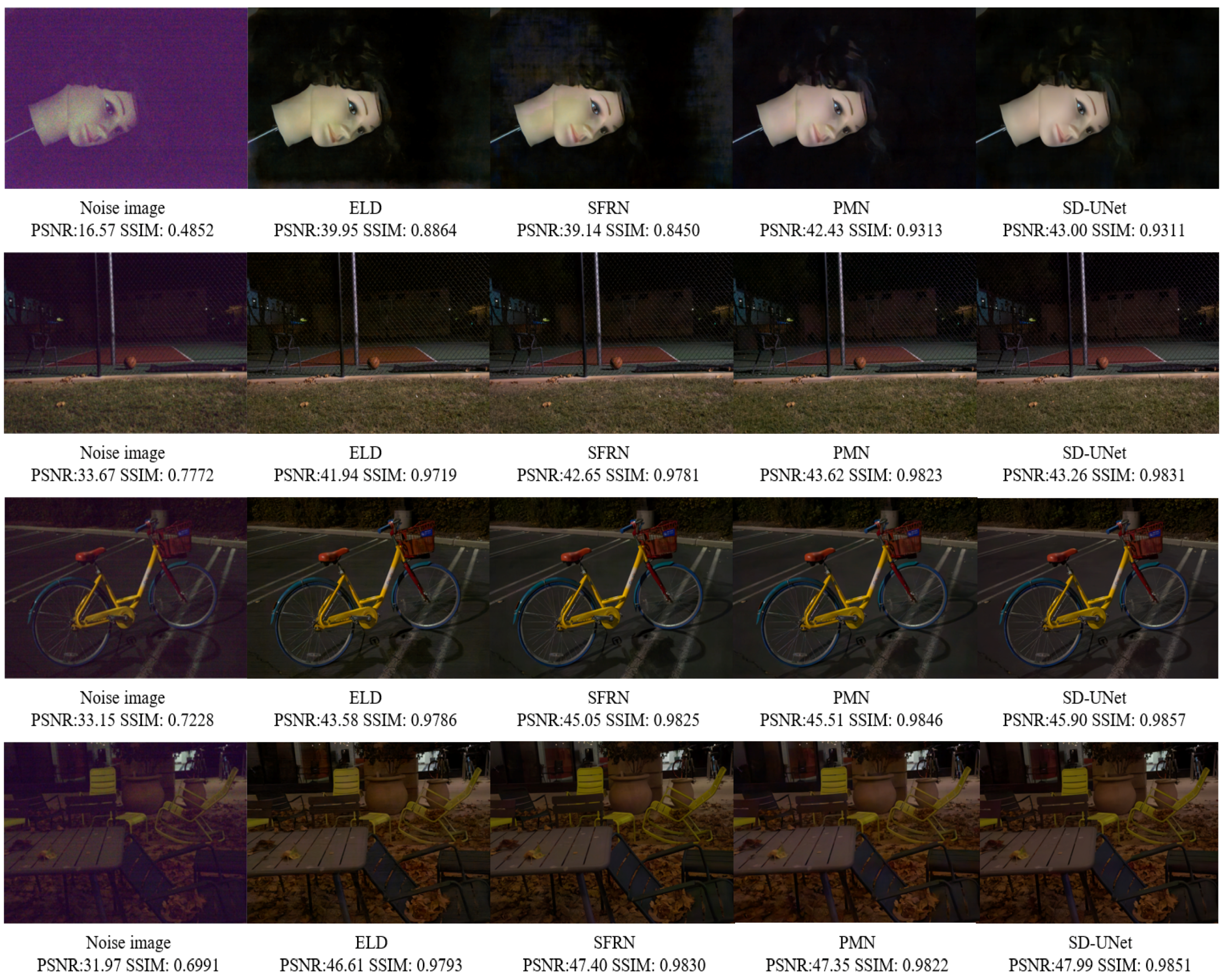
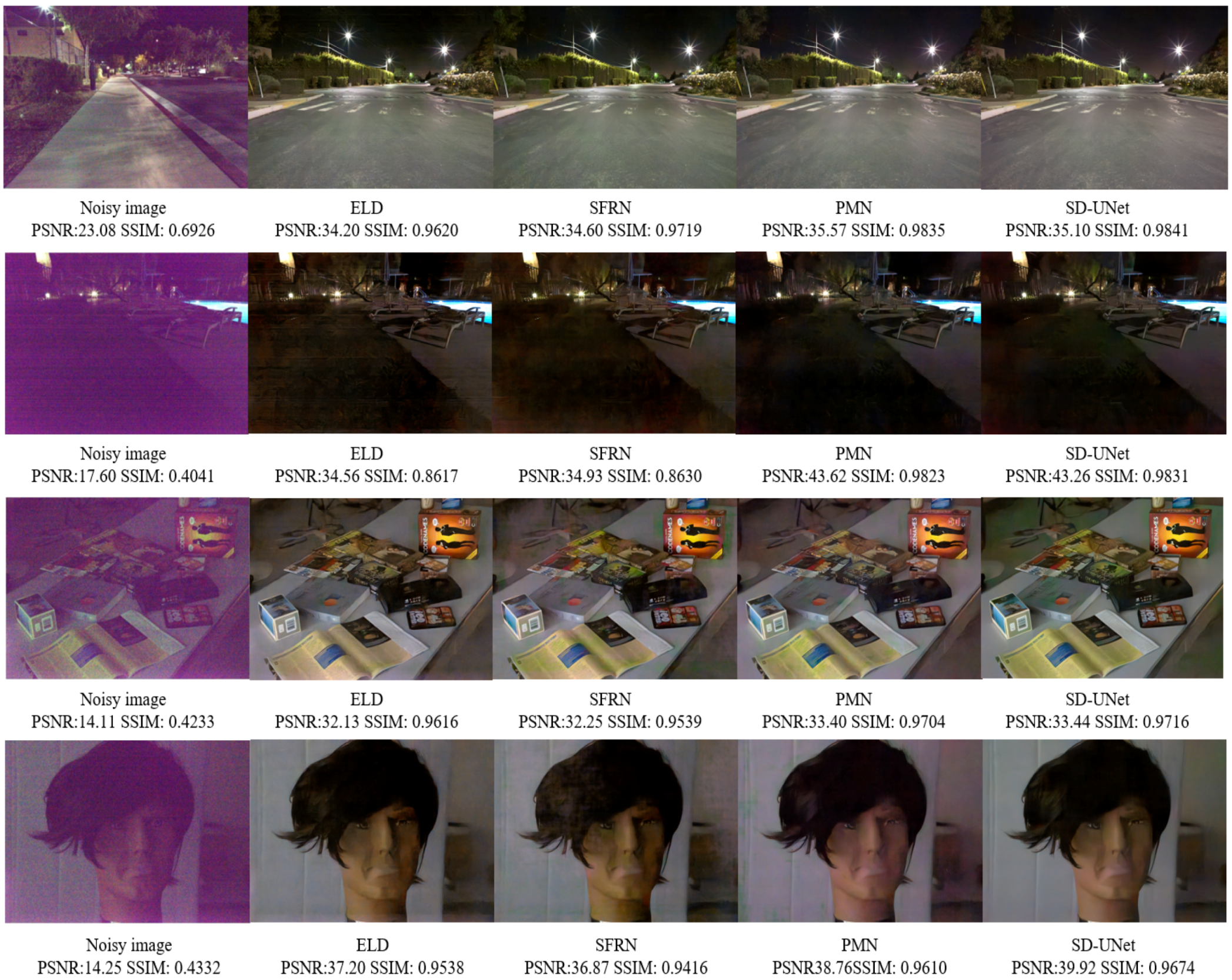
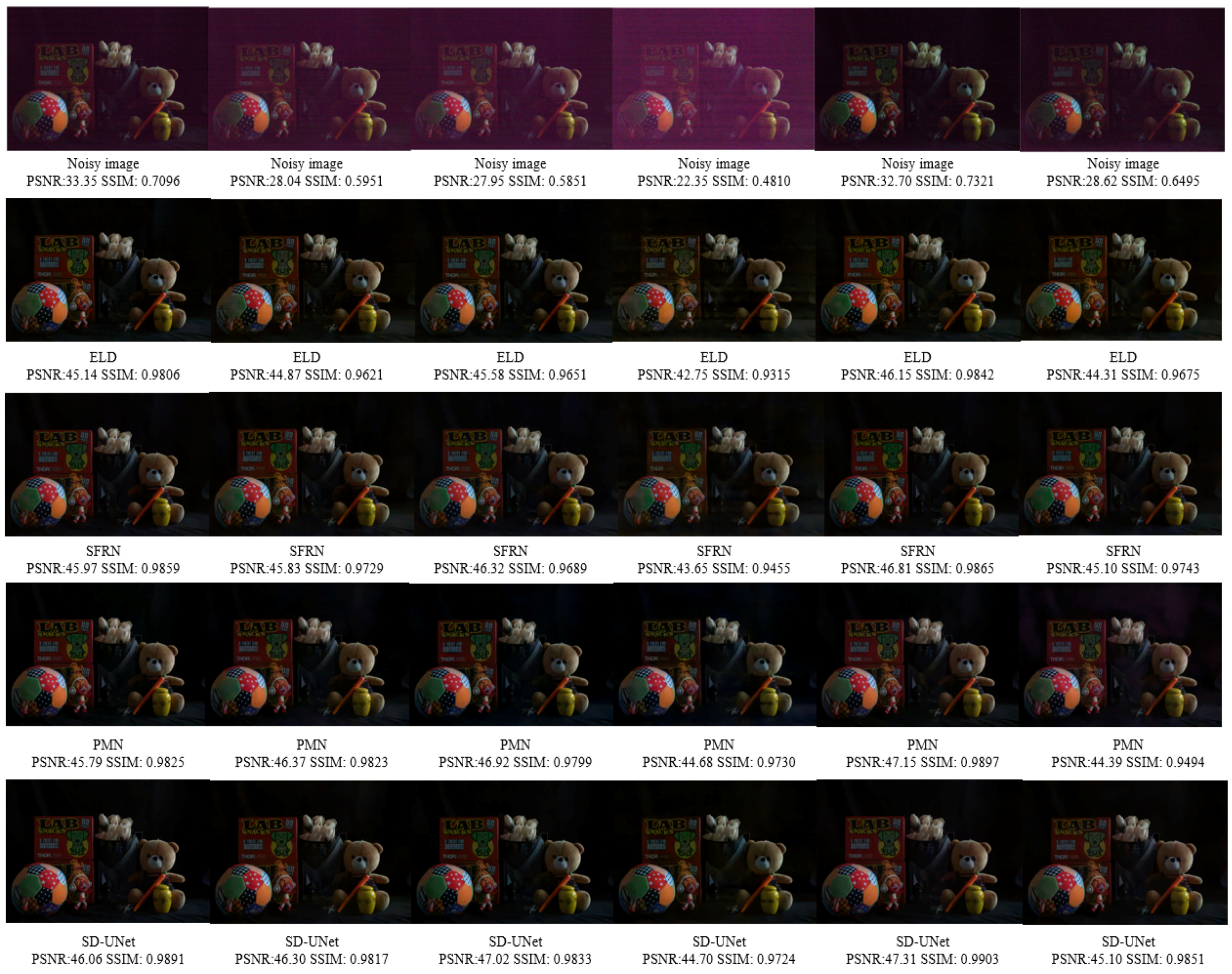
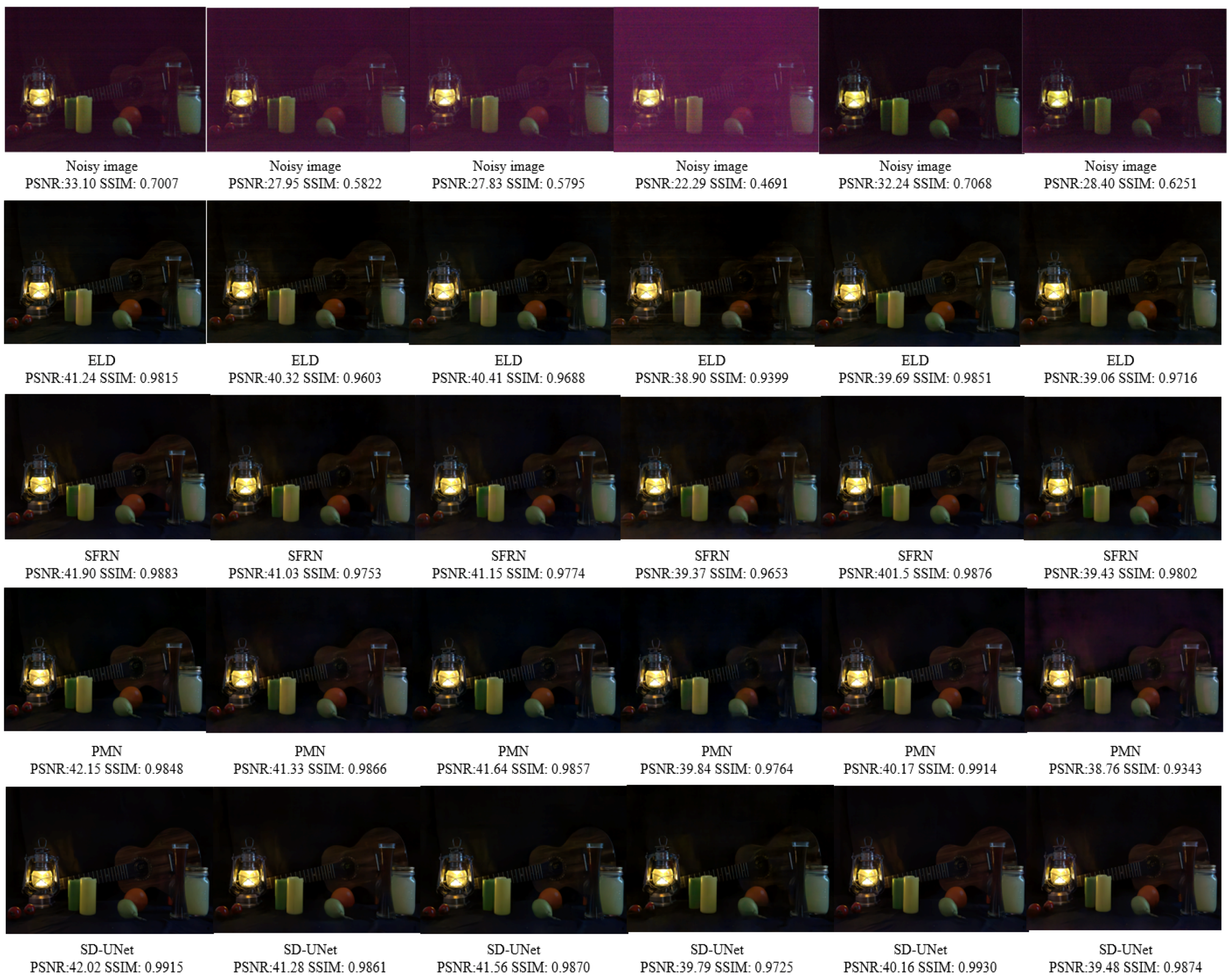
4.6. Visual Results Analysis

In order to further evaluate the effectiveness of SD-UNet, multiple images are selected from the SID dataset with different low-light factors. The corresponding denoised results are shown in Figure 9, Figure 10 and Figure 11 along with several other SOTA low-light denoising methods. The corresponding evaluation indexes of denoised images are also shown below each figure. It is easy to see that the shorter the exposure time, the more noise is included in the image. In addition, the proposed SD-UNet can achieve a more comprehensive visual performance on all kinds of images captured under different low-light factors compared to existing methods.

The visual performance comparison on the ELD dataset is shown in Figure 12 and Figure 13. Unlike SID, the ELD dataset contains images captured under different ISO settings, under different low-light factors and with different camera equipment. Each figure contains a series of noisy images from one scene. Similar to the SID dataset, each noisy image has a corresponding long-exposure image as the ground truth image, and the evaluation index for each image is also shown in the results. From the experimental results, one can easily see that the proposed SD-UNet demonstrates an improvement compared with ELD and SNFR and is very competitive with PMN. The denoising performance shows that the proposed SD-UNet has a good noise modeling ability and can extract outstanding noise representations.

Finally, as seen from the visual results, the proposed SD-UNet acquires very clean texture information and realistic color distributions for both the SID and ELD datasets, which further proves that it has an excellent noise modeling ability and denoising performance.

5. Conclusions

In this paper, a novel deep learning model, termed SD-UNet, is proposed to tackle the low-light image denoising task. By analyzing the visual characteristics of noise patterns, multiple strategies are applied on the conventional U-Net structure to improve the noise distribution modeling ability. Firstly, a deformable convolution with a flexible receptive field is applied to deal with noise patterns with various geometries; next, a self-adaptive learning block is leveraged to help the network automatically select appropriate scales and extract reliable noise distribution representations. Finally, a novel structural loss function is proposed to model the geometric structure of the denoised and ground truth images so as to guide the parameter optimization process in a more efficient way. The experimental results on both SID and ELD datasets established the effectiveness of the proposed method.

References

1. Hasinoff, S.W.; Sharlet, D.; Geiss, R.; Adams, A.; Barron, J.T.; Kainz, F.; Chen, J.; Levoy, M. Burst photography for high dynamic range and low-light imaging on mobile cameras. ACM Trans. Graph. (ToG) 2016, 35, 1–12. [Google Scholar] [CrossRef]
2. Liba, O.; Murthy, K.; Tsai, Y.T.; Brooks, T.; Xue, T.; Karnad, N.; He, Q.; Barron, J.T.; Sharlet, D.; Geiss, R.; et al. Handheld mobile photography in very low light. ACM Trans. Graph. 2019, 38, 164. [Google Scholar] [CrossRef]
3. Guerrieri, F.; Tisa, S.; Zappa, F. Fast single-photon imager acquires 1024 pixels at 100 kframe/s. In Proceedings of the Sensors, Cameras, and Systems for Industrial/Scientific Applications X, San Jose, CA, USA, 20–22 January 2009; Volume 7249, pp. 213–223. [Google Scholar]
4. Morris, P.A.; Aspden, R.S.; Bell, J.E.; Boyd, R.W.; Padgett, M.J. Imaging with a small number of photons. Nat. Commun. 2015, 6, 5913. [Google Scholar] [CrossRef] [PubMed]
5. Xu, J.; Zhang, L.; Zhang, D.; Feng, X. Multi-channel weighted nuclear norm minimization for real color image denoising. In Proceedings of the IEEE international Conference on Computer Vision, Venice, Italy, 22–29 October 2017; pp. 1096–1104. [Google Scholar]
6. Xu, J.; Zhang, L.; Zhang, D. A trilateral weighted sparse coding scheme for real-world image denoising. In Proceedings of the European conference on Computer Vision (ECCV), Munich, Germany, 8–14 September 2018; pp. 20–36. [Google Scholar]
7. Guo, S.; Yan, Z.; Zhang, K.; Zuo, W.; Zhang, L. Toward convolutional blind denoising of real photographs. In Proceedings of the IEEE/CVF Conference on Computer Vision and Pattern Recognition, Long Beach, CA, USA, 15–20 June 2019; pp. 1712–1722. [Google Scholar]
8. Brooks, T.; Mildenhall, B.; Xue, T.; Chen, J.; Sharlet, D.; Barron, J.T. Unprocessing images for learned raw denoising. In Proceedings of the IEEE/CVF Conference on Computer Vision and Pattern Recognition, Long Beach, CA, USA, 15–20 June 2019; pp. 11036–11045. [Google Scholar]
9. Foi, A.; Trimeche, M.; Katkovnik, V.; Egiazarian, K. Practical Poissonian–Gaussian noise modeling and fitting for single-image raw-data. IEEE Trans. Image Process. 2008, 17, 1737–1754. [Google Scholar] [CrossRef] [PubMed]
10. LeCun, Y.; Bengio, Y.; Hinton, G. Deep learning. Nature 2015, 521, 436–444. [Google Scholar] [CrossRef] [PubMed]
11. Krizhevsky, A.; Sutskever, I.; Hinton, G.E. ImageNet classification with deep convolutional neural networks. Commun. ACM 2017, 60, 84–90. [Google Scholar] [CrossRef]
12. Simonyan, K.; Zisserman, A. Very deep convolutional networks for large-scale image recognition. arXiv 2014, arXiv:1409.1556. [Google Scholar]
13. Zhang, Y.; Li, W.; Sun, W.; Tao, R.; Du, Q. Single-source domain expansion network for cross-scene hyperspectral image classification. IEEE Trans. Image Process. 2023, 32, 1498–1512. [Google Scholar] [CrossRef] [PubMed]
14. Bhatti, U.A.; Huang, M.; Neira-Molina, H.; Marjan, S.; Baryalai, M.; Tang, H.; Wu, G.; Bazai, S.U. MFFCG–Multi feature fusion for hyperspectral image classification using graph attention network. Expert Syst. Appl. 2023, 229, 120496. [Google Scholar] [CrossRef]
15. Liu, W.; Anguelov, D.; Erhan, D.; Szegedy, C.; Reed, S.; Fu, C.Y.; Berg, A.C. Ssd: Single shot multibox detector. In Proceedings of the Computer Vision–ECCV 2016: 14th European Conference, Amsterdam, The Netherlands, 11–14 October 2016; Proceedings, Part I 14. Springer: Berlin/Heidelberg, Germany, 2016; pp. 21–37. [Google Scholar]
16. Ren, S.; He, K.; Girshick, R.; Sun, J. Faster r-cnn: Towards real-time object detection with region proposal networks. Adv. Neural Inf. Process. Syst. 2015, 28, 1–9. [Google Scholar] [CrossRef] [PubMed]
17. Zou, Z.; Chen, K.; Shi, Z.; Guo, Y.; Ye, J. Object detection in 20 years: A survey. Proc. IEEE 2023, 111, 257–276. [Google Scholar] [CrossRef]
18. Chen, S.; Sun, P.; Song, Y.; Luo, P. Diffusiondet: Diffusion model for object detection. In Proceedings of the IEEE/CVF International Conference on Computer Vision, Paris, France, 1–6 October 2023; pp. 19830–19843. [Google Scholar]
19. Wang, Z.; Li, Y.; Chen, X.; Lim, S.N.; Torralba, A.; Zhao, H.; Wang, S. Detecting everything in the open world: Towards universal object detection. In Proceedings of the IEEE/CVF Conference on Computer Vision and Pattern Recognition, Paris, France, 1–6 October 2023; pp. 11433–11443. [Google Scholar]
20. Chen, L.C.; Papandreou, G.; Kokkinos, I.; Murphy, K.; Yuille, A.L. Deeplab: Semantic image segmentation with deep convolutional nets, atrous convolution, and fully connected crfs. IEEE Trans. Pattern Anal. Mach. Intell. 2017, 40, 834–848. [Google Scholar] [CrossRef] [PubMed]
21. He, K.; Gkioxari, G.; Dollár, P.; Girshick, R. Mask r-cnn. In Proceedings of the IEEE International Conference on Computer Vision, Venice, Italy, 22–29 October 2017; pp. 2961–2969. [Google Scholar]
22. Jain, J.; Li, J.; Chiu, M.T.; Hassani, A.; Orlov, N.; Shi, H. Oneformer: One transformer to rule universal image segmentation. In Proceedings of the IEEE/CVF Conference on Computer Vision and Pattern Recognition, Vancouver, BC, Canada, 17–24 June 2023; pp. 2989–2998. [Google Scholar]
23. Wu, J.; Fu, R.; Fang, H.; Zhang, Y.; Yang, Y.; Xiong, H.; Liu, H.; Xu, Y. Medsegdiff: Medical image segmentation with diffusion probabilistic model. In Proceedings of the Medical Imaging with Deep Learning, PMLR, Paris, France, 3–5 July 2024; pp. 1623–1639. [Google Scholar]
24. Jang, G.; Lee, W.; Son, S.; Lee, K.M. C2n: Practical generative noise modeling for real-world denoising. In Proceedings of the IEEE/CVF International Conference on Computer Vision, Montreal, QC, Canada, 10–17 October 2021; pp. 2350–2359. [Google Scholar]
25. Maleky, A.; Kousha, S.; Brown, M.S.; Brubaker, M.A. Noise2noiseflow: Realistic camera noise modeling without clean images. In Proceedings of the IEEE/CVF Conference on Computer Vision and Pattern Recognition, New Orleans, LA, USA, 18–24 June 2022; pp. 17632–17641. [Google Scholar]
26. Zhang, Y.; Qin, H.; Wang, X.; Li, H. Rethinking noise synthesis and modeling in raw denoising. In Proceedings of the IEEE/CVF International Conference on Computer Vision, Montreal, QC, Canada, 10–17 October 2021; pp. 4593–4601. [Google Scholar]
27. Chen, C.; Chen, Q.; Do, M.N.; Koltun, V. Seeing motion in the dark. In Proceedings of the IEEE/CVF International Conference on Computer Vision, Seoul, Republic of Korea, 27 October–2 November 2019; pp. 3185–3194. [Google Scholar]
28. Monakhova, K.; Richter, S.R.; Waller, L.; Koltun, V. Dancing under the stars: Video denoising in starlight. In Proceedings of the IEEE/CVF Conference on Computer Vision and Pattern Recognition, New Orleans, LA, USA, 18–24 June 2022; pp. 16241–16251. [Google Scholar]
29. Moseley, B.; Bickel, V.; López-Francos, I.G.; Rana, L. Extreme low-light environment-driven image denoising over permanently shadowed lunar regions with a physical noise model. In Proceedings of the IEEE/CVF Conference on Computer Vision and Pattern Recognition, Nashville, TN, USA, 20–25 June 2021; pp. 6317–6327. [Google Scholar]
30. Wang, J.; Yu, Y.; Wu, S.; Lei, C.; Xu, K. Rethinking noise modeling in extreme low-light environments. In Proceedings of the 2021 IEEE International Conference on Multimedia and Expo (ICME), Shenzhen, China, 5–9 July 2021; pp. 1–6. [Google Scholar]
31. Wei, K.; Fu, Y.; Zheng, Y.; Yang, J. Physics-based noise modeling for extreme low-light photography. IEEE Trans. Pattern Anal. Mach. Intell. 2021, 44, 8520–8537. [Google Scholar] [CrossRef] [PubMed]
32. Cao, Y.; Liu, M.; Liu, S.; Wang, X.; Lei, L.; Zuo, W. Physics-guided iso-dependent sensor noise modeling for extreme low-light photography. In Proceedings of the IEEE/CVF Conference on Computer Vision and Pattern Recognition, Vancouver, BC, Canada, 17–24 June 2023; pp. 5744–5753. [Google Scholar]
33. Chang, K.C.; Wang, R.; Lin, H.J.; Liu, Y.L.; Chen, C.P.; Chang, Y.L.; Chen, H.T. Learning camera-aware noise models. In Proceedings of the European Conference on Computer Vision, Glasgow, UK, 23–28 August 2020; pp. 343–358. [Google Scholar]
34. Abdelhamed, A.; Lin, S.; Brown, M.S. A high-quality denoising dataset for smartphone cameras. In Proceedings of the IEEE Conference on Computer Vision and Pattern Recognition, Salt Lake City, UT, USA, 18–23 June 2018; pp. 1692–1700. [Google Scholar]
35. Feng, H.; Wang, L.; Wang, Y.; Huang, H. Learnability enhancement for low-light raw denoising: Where paired real data meets noise modeling. In Proceedings of the 30th ACM International Conference on Multimedia, Lisboa, Portugal, 10–14 October 2022; pp. 1436–1444. [Google Scholar]
36. Chen, C.; Chen, Q.; Xu, J.; Koltun, V. Learning to see in the dark. In Proceedings of the IEEE Conference on Computer Vision and Pattern Recognition, Salt Lake City, UT, USA, 18–23 June 2018; pp. 3291–3300. [Google Scholar]
37. Ronneberger, O.; Fischer, P.; Brox, T. U-net: Convolutional networks for biomedical image segmentation. In Proceedings of the Medical Image Computing and Computer-Assisted Intervention–MICCAI 2015: 18th International Conference, Munich, Germany, 5–9 October 2015; Proceedings, Part III 18. Springer: Berlin/Heidelberg, Germany, 2015; pp. 234–241. [Google Scholar]
38. Janesick, J.; Klaasen, K.; Elliott, T. CCD charge collection efficiency and the photon transfer technique. In Proceedings of the Solid-State Imaging Arrays, San Diego, CA, USA, 22–23 August 1985; Volume 570, pp. 7–19. [Google Scholar]
39. Joiner, B.L.; Rosenblatt, J.R. Some properties of the range in samples from Tukey’s symmetric lambda distributions. J. Am. Stat. Assoc. 1971, 66, 394–399. [Google Scholar] [CrossRef]
40. Gow, R.D.; Renshaw, D.; Findlater, K.; Grant, L.; McLeod, S.J.; Hart, J.; Nicol, R.L. A comprehensive tool for modeling CMOS image-sensor-noise performance. IEEE Trans. Electron Devices 2007, 54, 1321–1329. [Google Scholar] [CrossRef]
41. Abdelhamed, A.; Brubaker, M.A.; Brown, M.S. Noise flow: Noise modeling with conditional normalizing flows. In Proceedings of the IEEE/CVF International Conference on Computer Vision, Seoul, Republic of Korea, 27 October–2 November 2019; pp. 3165–3173. [Google Scholar]
42. Wang, J.; Li, P.; Deng, J.; Du, Y.; Zhuang, J.; Liang, P.; Liu, P. CA-GAN: Class-condition attention GAN for underwater image enhancement. IEEE Access 2020, 8, 130719–130728. [Google Scholar] [CrossRef]
43. Zhu, J.Y.; Park, T.; Isola, P.; Efros, A.A. Unpaired image-to-image translation using cycle-consistent adversarial networks. In Proceedings of the IEEE International Conference on Computer Vision, Venice, Italy, 22–29 October 2017; pp. 2223–2232. [Google Scholar]
44. Anoosheh, A.; Sattler, T.; Timofte, R.; Pollefeys, M.; Van Gool, L. Night-to-day image translation for retrieval-based localization. In Proceedings of the 2019 International Conference on Robotics and Automation (ICRA), Montreal, QC, Canada, 20–24 May 2019; pp. 5958–5964. [Google Scholar]
45. Isola, P.; Zhu, J.Y.; Zhou, T.; Efros, A.A. Image-to-image translation with conditional adversarial networks. In Proceedings of the IEEE Conference on Computer Vision and Pattern Recognition, Honolulu, HI, USA, 21–26 July 2017; pp. 1125–1134. [Google Scholar]
46. Lakmal, H.; Dissanayake, M. Illuminating the Roads: Night-to-Day Image Translation for Improved Visibility at Night. In Proceedings of the International Conference on Asia Pacific Advanced Network, Colombo, Sri Lanka, 24–25 August 2023; pp. 13–26. [Google Scholar]
47. Zamir, S.W.; Arora, A.; Khan, S.; Hayat, M.; Khan, F.S.; Yang, M.H.; Shao, L. Learning enriched features for fast image restoration and enhancement. IEEE Trans. Pattern Anal. Mach. Intell. 2022, 45, 1934–1948. [Google Scholar] [CrossRef] [PubMed]
48. Canny, J. A computational approach to edge detection. IEEE Trans. Pattern Anal. Mach. Intell. 1986, PAMI-8, 679–698. [Google Scholar] [CrossRef]
49. Wang, Z.; Bovik, A.C.; Sheikh, H.R.; Simoncelli, E.P. Image quality assessment: From error visibility to structural similarity. IEEE Trans. Image Process. 2004, 13, 600–612. [Google Scholar] [CrossRef] [PubMed]
50. Kingma, D.P.; Ba, J. Adam: A method for stochastic optimization. arXiv 2014, arXiv:1412.6980. [Google Scholar]
Figure 1. The overall structure of the proposed SD-UNet.
Symmetry 16 00646 g001
Figure 2. The comparison between traditional 3 3 convolution and deformable convolution. The left is the 3 3 convolution kernel. Each of its nine positions is denoted as P n {(−1,−1), (−1,0), …, (0,1), (1,1)}. The orange dots centered on P 0 represent the original range of convolution sampling positions on the feature map. The orange arrows denote the learned offsets Δ P n , and the blue dots denote the actual deformable convolution sampling positions after offsetting.
Symmetry 16 00646 g002
Figure 3. The structure of the proposed SLAB.
Symmetry 16 00646 g003
Figure 4. The structure of proposed dilated deformable convolution.The orange dots centered on P 0 represent the original range of convolution sampling positions on the feature map. The orange arrows denote the learned offsets Δ P n , and the blue dots denote the actual deformable convolution sampling positions after offsetting.The green area represents the convolution operation position corresponding to the traditional convolution operations, while the yellow area represents the convolution operation position corresponding to dilated convolution operations.
Symmetry 16 00646 g004
Figure 5. The PSNR and SSIM distribution for the SID dataset.
Symmetry 16 00646 g005
Figure 6. The visual comparison for the ablation study.
Symmetry 16 00646 g006
Figure 7. The training curve of the proposed loss function and L1 loss.
Symmetry 16 00646 g007
Figure 8. The PSNR and SSIM distribution for the ELD dataset.
Symmetry 16 00646 g008
Figure 9. Comparison of the proposed method and multiple SOTA methods on SID ×100.
Symmetry 16 00646 g009
Figure 10. Comparison of the proposed method and multiple SOTA methods on SID ×250.
Symmetry 16 00646 g010
Figure 11. Comparison of the proposed method and multiple SOTA methods on SID ×300.
Symmetry 16 00646 g011
Figure 12. Comparison of the proposed method and multiple SOTA methods on ELD Scene 1.
Symmetry 16 00646 g012
Figure 13. Comparison of the proposed method and multiple SOTA methods on ELD Scene 7.
Symmetry 16 00646 g013